DUCK: Distance-based Unlearning via Centroid Kinematics

Abstract

Machine Unlearning is rising as a new field, driven by the pressing necessity of ensuring privacy in modern artificial intelligence models. This technique primarily aims to eradicate any residual influence of a specific subset of data from the knowledge acquired by a neural model during its training. This work introduces a novel unlearning algorithm, denoted as Distance-based Unlearning via Centroid Kinematics (DUCK), which employs metric learning to guide the removal of samples matching the nearest incorrect centroid in the embedding space. Evaluation of the algorithm’s performance is conducted across various benchmark datasets in two distinct scenarios, class removal, and homogeneous sampling removal, obtaining state-of-the-art performance. We introduce a novel metric, called Adaptive Unlearning Score (AUS), encompassing not only the efficacy of the unlearning process in forgetting target data but also quantifying the performance loss relative to the original model. Moreover, we propose a novel membership inference attack to assess the algorithm’s capacity to erase previously acquired knowledge, designed to be adaptable to future methodologies.

Code is publicly available at https://github.com/OcraM17/DUCK.

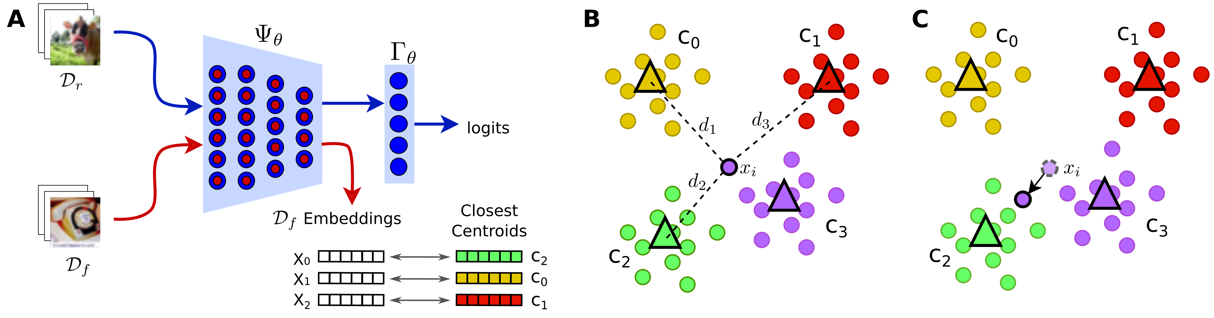
Figure 1: DUCK unlearning scheme. A) DUCK architecture $\Phi_{\theta}=\Gamma_{\theta}\circ\Psi_{\theta}$ during unlearnig phase. The weights of $\Gamma_{\theta}$ are updated through gradient descent using $\mathcal{L}_{RET}$ loss on $\mathcal{D}_{r}$. Importantly, weights of $\Psi_{\theta}$ are optimized using both the gradient obtained from $\Gamma_{\theta}$ and also from the closest-centroid matching applied on $\mathcal{D}_{f}$. B) Representation of Phase-I closest-centroid matching, where for each sample $x_{i}\in\mathcal{D}_{f}$ is computed its distance from incorrect classes centroids and the closest is selected. C) Phase-II, the distance between $x_{i}$ and the selected closest centroid is minimized through gradient descent.

1 Introduction

In the ever-evolving landscape of artificial intelligence and machine learning, the development of algorithms capable of learning and adapting to data has garnered significant attention. The ascent of artificial intelligence enabled remarkable achievements in various domains, however, the use of machine learning systems comes with some privacy challenges.
Machine learning models, once trained, store in their parameters the patterns and information from the data they have been exposed to. Unfortunately, this persistence of learned information can lead to unintended consequences, from privacy breaches due to lingering personal data, to biased decisions rooted in historical biases present in the training data.

For instance, the information extraction can be performed by a malicious attacker through several procedures [39, 35, 40, 47, 28, 15]. Similarly, the injection of adversarial data can force machine learning models to output wrong predictions resulting in serious security problems [34, 4, 25]. Last but not least, numerous recent privacy-preserving regulations, have been enacted, such as the European Union’s General Data Protection Regulation[24] and the California Consumer Privacy Act [30]. Under these regulations, users are entitled to request the deletion of their data and related information to safeguard their privacy. Hence, a procedure to remove selectively part of the information stored in the parameters of the models represents a fundamental open problem.
To this end, Machine Unlearning studies methodologies to instill selective forgetting in trained models such that training data or sensitive information can not be recovered [28, 45, 37, 27, 44]. In the context of an original model trained on a dataset, unlearning approaches seek to eliminate information about a specific subset of data, termed the forget-set, from the parameters of the original network while preserving its generalization performance. Crucially, the information removal process from the original model involves ensuring that the unlearned model makes identical predictions to a new model trained from scratch on the retained dataset (i.e., the dataset without the forget-set).
Motivated by the growing need for more precise privacy-preserving unlearning methods, this paper introduces DUCK, a novel methodology that leverages metric learning. During the unlearning steps, DUCK initially computes centroids in the embedding space for each class in the dataset. Then, it minimizes the distance between the embeddings of forget-samples and the incorrect-class closest centroid. Importantly, DUCK can adapt to different unlearning scenarios such as class-removal or homogeneous sampling removal tasks, where the model has to discard entire classes in the former or the model unlearns a random subset of the training set in the latter.

The main contributions of this paper can be summarized as:

• Introduction of a novel machine unlearning method, Distance-based Unlearning via Centroid Kinematics DUCK, that employs metric learning to guide the removal of samples information from the model’s knowledge. This involves directing samples towards the nearest incorrect centroid in the multidimensional space.

• Development of a novel metric, the Adaptive Unlearning Score (AUS), designed to quantify the trade-off between the forget-set accuracy and the overall test accuracy of the unlearned model.

• Introduction of a novel Membership Inference Attack (MIA) using a robust classifier to verify the forget-set data privacy protection ( i.e. to assess the correct removal of the forget-set information from the model). Privacy leakage detection is achieved by exploiting the informational content of the logits of the unlearned model.

• Comprehensive experimental evaluations have been conducted on four publicly available datasets and against several related methods from the state-of-the-art.

2 Related Works

A recent growth of concerns about privacy issues in deep learning algorithms [6, 38, 1] is leading to a notable surge in the development of machine unlearning methods. In this section, we provide a review of recent works closely aligned with our proposed solution. Machine unlearning methods are designed to eliminate information associated with a specific subset of training data from the weights of a neural model while maintaining the performance of the model on the remaining data. These methods can be classified into two primary groups based on their approach: exact data removal [2, 26, 46] and approximate methods [12, 42, 11, 10]. The former aims to deterministically remove information from the forget-set, while the latter optimizes a loss function stochastically to unlearn the forget-set.
Within these two categories, methods can be further subdivided based on their specific removal algorithms. For instance, in [22, 36, 41], authors performed unlearning strategies on adversarially trained models. Recent studies such as [18, 16] have leveraged contrastive learning techniques to discard the information regarding the forget-set. Another set of methodologies addresses unlearning by utilizing either a limited subset of training samples (Few-Shot approaches [48, 33]) or, in a more challenging setting, no training samples at all (Zero-Shot approaches [8]). These approaches represent diverse perspectives in handling unlearning scenarios, highlighting the adaptability of techniques to different data constraints and learning paradigms. Other notable methods are based on Adaptive unlearning [13, 2] or Hierarchical unlearning [49]. The first approach tailors the unlearning strategy to the input dataset and model, aiming to make the unlearning strategy adaptable and consistent. The latter, after partitioning and sorting the dataset, trains multiple sub-models for each partition. In case of unlearning requests, it retrains the sub-model that contains the point to forget. Recently, two algorithms based on manipulating the decision boundary to remove entire classes have been proposed in [7]. Finally, in [20], the authors present a two-phase method for knowledge removal. This method involves learning distinct masks that are applied independently to the neural model, each corresponding to a specific class within the dataset. Thanks to these masks, the unlearning strategy can remove information about determined classes. Then, during the second phase, it can recover information about the data points to retain.

3 Methods

In this section, we present a definition of the machine unlearning problem and how our solution, DUCK, can be applied to a general deep learning architecture to induce the forgetting of a subset of data from the training set.

Preliminaries.   Given a classification task and a dataset $\{x_{i},y_{i}\}^{N}_{i=1}$ where $x_{i}$ denotes images, and $y_{i}$ represents their corresponding labels. The label values $y_{i}$ fall within the range $\{0,\dots,K-1\}$, where $K$ is the total number of classes in the dataset. Typically, this dataset is partitioned into two subsets: the training set $\mathcal{D}$ and the test set $\mathcal{D}^{t}$.

When there is a request to remove a specific class $C$ from $\mathcal{D}$, a machine unlearning algorithm must be applied to the original classification model $\Phi_{\theta}$ trained on $\mathcal{D}$. This approach aims to eliminate the information about class $C$ from the model weights $\theta$. We term this unlearning task as the Class-Removal (CR) scenario. In CR, the two sets $\mathcal{D}$ and $\mathcal{D}^{t}$ are divided into retain-sets ($\mathcal{D}_{r}$, $\mathcal{D}^{t}_{r}$) and forget-sets ($\mathcal{D}_{f}$, $\mathcal{D}^{t}_{f}$). The retain-sets contain all instances of images that should be preserved, denoted as $\mathcal{D}r=\{x^{r}_{i},y^{r}_{i}\}_{i=1}^{N^{r}}$, with $y^{r}_{i}\in\{0,\dots,K-1\}\setminus\{C\}$. Conversely, the forget-sets contain only the images associated with the class label to be removed, i.e., $\mathcal{D}_{f}=\{x^{f}_{i},y^{f}_{i}\}^{N^{f}}_{i=1}$ with $y^{f}_{i}\in\{C\}$. Ideally, through the utilization of these sets, the unlearned model $\Phi_{\theta}^{U}$ should achieve performance on the test set akin to that of an “oracle” model trained solely on the retain-set $\mathcal{D}_{r}$. This entails maximizing accuracy on $\mathcal{D}^{t}_{r}$ while being completely unaware of $\mathcal{D}^{t}_{f}$.

We also considered an alternative unlearning scenario defined as Homogeneous Removal (HR). This approach involves uniformly sampling from the dataset $\mathcal{D}$ to create a subset of data called $\mathcal{D}_{f}$, which comprises the samples intended for removal. The unlearning algorithm’s objective is to forget specific samples $x_{i}\in\mathcal{D}_{f}$ from the training set so that they are indistinguishable from images from $\mathcal{D}^{t}$ while aiming to maintain the original model’s performance on the test set $\mathcal{D}^{t}$ to the greatest extent possible.

Unlike CR, the HR scenario has distinct characteristics. It requires maintaining general knowledge about classes, resulting in a more targeted removal of information. However, precision is crucial in eliminating specific information related to the forget-samples. Notably, in the HR scenario, the test set $\mathcal{D}^{t}$ is not divided into retain and forget subsets. This is because the unlearned model should sustain its generalization capabilities for each class, affected by the removal of $\mathcal{D}_{f}$ samples. The remaining data from the training set are defined as $\mathcal{D}_{r}=\mathcal{D}\setminus\mathcal{D}_{f}$.

Proposed Method   Given an original model $\Phi_{\theta}$, our approach aims to erase the information pertaining to the forget-set samples from the model weights $\theta$, directly influencing the feature vectors derived from $\Phi_{\theta}$. The network $\Phi_{\theta}$ can be represented as $\Gamma_{\theta}\circ\Psi_{\theta}$, where $\Psi_{\theta}$ constitutes the backbone of the network, typically encompassing convolutional layers in the case of a CNN, while $\Gamma_{\theta}$ represents the last fully-connected layer of the network (Fig. 1A).

Prior to the optimization procedure, the algorithm calculates the centroid vector $c_{i}$ in the embeddings space for each class in $\mathcal{D}_{r}$. This involves computing $c_{i}$ as the mean embedding vector, as detailed in eq. 1.

$$c_{i}=\frac{1}{N_{i}}\sum_{j=0}^{N_{i}-1}\Psi_{\theta}(x_{j})$$ (1)

where $N_{i}$ is the number of samples in $\mathcal{D}_{r}$ for the $i^{\text{th}}$-class.

After retrieving the centroids, the optimization procedure calculates the forget-loss from forget-set batches and the retain-loss from retain-set batches. The forget-loss computation consists of two phases: closest-centroid matching and distance computation. During the first phase (phase-I, Fig. 1A-B), for each sample in the forget-set batch $(x_{j},y_{j})$, DUCK selects the centroid in $\{c_{i}\}_{i=0}^{K-1}$ belonging to a class different from $y_{j}$ that minimizes the pairwise cosine distance $d$ from $\Psi_{\theta}(x_{j})$, as defined in eq. 2.

$$c^{*}_{j}=\min\limits_{c_{i}}d(\Psi_{\theta}(x_{j}),c_{i})$$ (2)

Phase-I of the algorithm is crucial as it determines the optimal directions for moving the embeddings of forget-samples.

Subsequently, in the phase-II (Fig. 1C), the loss is computed by assessing the cosine distances between the embeddings $\Psi_{\theta}(x_{j})$ and the selected closest centroid $c^{*}_{j}$ as follows:

$$\mathcal{L}_{FGT}=\frac{1}{N_{\text{batch}}}\sum_{j=0}^{N_{\text{batch}}-1}1-\frac{\Psi_{\theta}(x_{j})\cdot c^{*}_{j}}{||\Psi_{\theta}(x_{j})||\;||c^{*}_{j}||},$$ (3)

where $N_{\text{batch}}$ is the number of forget samples in the batch.

Minimizing this loss involves moving the extracted embeddings of forget-samples away from the correct class centroid and toward the closest incorrect class centroid. This compels $\Psi_{\theta}$ to recognize unreliable and unnecessary features from these samples (the impact of the unlearning algorithm on the position of the embeddings in the latent space is discussed in Sec 4.5).

The retain-loss considers the entire network $\Phi_{\theta}=\Gamma_{\theta}\circ\Psi_{\theta}$ and entails computing the cross-entropy loss of the retain-set batch samples $(x_{j},y_{j})$, as expressed in eq. 4.

$$\mathcal{L}_{RET}=\frac{1}{N_{\text{batch}}}\sum_{j=0}^{N_{\text{batch}}-1}\sum_{i=0}^{K-1}y_{i}log(p_{i,j})$$ (4)

where $K$ is the number of classes, $N_{\text{batch}}$ is the number of retain samples in the batch, $y_{i}$ the true label and $p_{i,j}$ is the probability of the $i^{th}$ class obtained from $\texttt{softmax}\left[\Gamma_{\theta}\circ\Psi_{\theta}(x_{j})\right]$. This loss serves as a knowledge-preserving method for the unlearning algorithm since it counterbalances the effect of the $\mathcal{L}_{FGT}$ on the backbone $\Psi_{\theta}$ weights (in Sec 4.4 we analyze the impact of the components of the loss function in an ablation study).

Finally, the overall loss is computed as a weighted combination of $\mathcal{L}_{FGT}$ and $\mathcal{L}_{RET}$ eq. 5

$$\mathcal{L}=\lambda_{1}\mathcal{L}_{FGT}+\lambda_{2}\mathcal{L}_{RET}$$ (5)

where $\lambda_{1}$ and $\lambda_{2}$ are hyperparameters.
The number of epochs in the unlearning algorithm is not predetermined; instead, it depends on the accuracy $\mathcal{A}_{f}$ on the train forget-set $\mathcal{D}_{f}$ computed at the conclusion of each epoch. The optimal $\mathcal{A}^{\star}_{f}$ accuracy is chosen based on the CR or HR scenarios. Once the computed $\mathcal{A}_{f}$ accuracy falls below the optimal value, the unlearning process is halted. The optimal accuracies $\mathcal{A}^{\star}_{f}$ are set at 1$\%$ for the CR scenario and are equal to the original model test accuracy $\mathcal{A}^{t}_{Or}$ for the HR scenario.
Another critical aspect of DUCK is the ratio between the number of batches available for the forget and retain-sets. The retain-set is typically significantly larger in both CR and HR scenarios than the forget-set. Consequently, the number of retain-set samples is restricted by configuring the number of available retain batches as a multiple (batch-ratio $\geq 1$) of the number of forget batches. The pseudocode for our unlearning method is outlined in Algorithm 1.

Algorithm 1 DUCK Pseudocode

Input: $\mathcal{D}_{r}$, $\mathcal{D}_{f}$, $\Phi_{\theta}=\Gamma_{\theta}\circ\Psi_{\theta}$, $\mathcal{A}^{\star}_{f}$, batch-ratio

Output: unlearned model $\Phi^{U}_{\theta}$

Compute centroids $c_{i}$ from $\Psi_{\theta}$ applied on $\mathcal{D}_{r}$

while $\mathcal{A}_{f}<\mathcal{A}^{\star}_{f}$ do

     for $(x^{f}_{j},y^{f}_{j})$ in $\mathcal{D}_{f}$ do

         for batch-iter $(x^{r}_{j},y^{r}_{j})$ in $\mathcal{D}_{r}$ do

              if batch-iter $<$ batch-ratio then

                  Compute closest centroid $c^{*}_{j}$ of $x^{f}_{j}$

                  Compute cosine distances: $d(\Psi_{\theta}(x^{f}_{j});c^{*}_{j})$

                  Compute $\mathcal{L}_{FGT}$

                  Compute cross-entropy loss $\mathcal{L}_{RET}$

                  Compute $\mathcal{L}=\lambda_{1}\mathcal{L}_{RET}+\lambda_{2}\mathcal{L}_{RET}$

                  Update weights $\theta$ using gradient descent

              end if

         end for

     end for

     Compute the unlearned model $\mathcal{A}_{f}$ on $\mathcal{D}_{f}$

end while

4 Experimental Results

In this section, we present the results of experiments conducted on four distinct datasets sourced from state-of-the-art research. We compared our method with others in the field, focusing on the two scenarios introduced earlier (CR and HR). Subsequently, we provide various analyses conducted to evaluate the effectiveness of our unlearning approach.

Table 1: Comparison between DUCK and methods from the state-of-the-art for CR scenario. The metrics reported here $\mathcal{A}_{r}$, $\mathcal{A}_{f}$, $\mathcal{A}^{t}_{r}$, $\mathcal{A}^{t}_{f}$, and AUS are mean $\pm$ std over ten runs where for each one of these a different class has been removed. ^† For ERM standard deviations are not available since the code released in [20] does not allow to remove classes arbitrarily; the results are reported for class 0.

	Metric	Original	Retrained	FineTuning	Neg. Grad	Rand. Lab.	Bound. Expanding	Bound. Shrink	ERM†	DUCK
CIFAR10	$\mathcal{A}_{r}$	99.46$\pm$00.05	99.69$\pm$00.12	100.00$\pm$00.00	83.55$\pm$02.59	72.93$\pm$08.79	92.24$\pm$02.51	93.54$\pm$02.10	83.62	95.49$\pm$00.89
	$\mathcal{A}_{f}$	99.42$\pm$00.43	00.00$\pm$00.00	00.00$\pm$00.00	00.00$\pm$00.00	00.64$\pm$00.15	15.56$\pm$03.41	14.76$\pm$05.49	00.00	00.00$\pm$00.00
	$\mathcal{A}_{r}^{t}$	88.64$\pm$00.63	88.05$\pm$01.28	87.93$\pm$01.14	76.27$\pm$03.27	65.46$\pm$07.59	82.36$\pm$02.39	83.81$\pm$02.29	80.31	85.53$\pm$01.37
	$\mathcal{A}_{f}^{t}$	88.34$\pm$00.62	00.00$\pm$00.00	00.00$\pm$00.00	00.56$\pm$00.12	00.83$\pm$00.44	13.34$\pm$03.21	13.64$\pm$03.57	00.00	00.00$\pm$00.00
	AUS	0.531$\pm$0.005	0.994$\pm$0.014	0.993$\pm$0.013	0.871$\pm$0.033	0.762$\pm$0.076	0.827$\pm$0.032	0.840$\pm$5.43	0.917	0.969$\pm$0.015
CIFAR100	$\mathcal{A}_{r}$	99.63$\pm$00.00	99.98$\pm$00.00	99.97$\pm$01.35	82.84$\pm$09.64	71.72$\pm$10.90	71.24$\pm$17.93	71.13$\pm$17.79	75.17	92.56$\pm$02.45
	$\mathcal{A}_{f}$	99.70$\pm$00.31	00.00$\pm$00.00	00.00$\pm$00.00	00.72$\pm$00.19	00.76$\pm$00.08	05.44$\pm$01.70	05.36$\pm$01.17	00.00	00.34$\pm$00.37
	$\mathcal{A}_{r}^{t}$	77.55$\pm$00.11	77.97$\pm$00.42	77.31$\pm$02.17	62.84$\pm$06.13	55.31$\pm$07.06	55.18$\pm$11.98	55.07$\pm$11.85	58.96	71.57$\pm$02.08
	$\mathcal{A}_{f}^{t}$	77.50$\pm$02.80	00.00$\pm$00.00	00.00$\pm$00.00	00.50$\pm$00.50	00.40$\pm$00.70	03.50$\pm$02.32	03.54$\pm$02.26	00.00	01.00$\pm$01.76
	AUS	0.563$\pm$0.009	1.004$\pm$0.022	0.998$\pm$0.022	0.849$\pm$0.061	0.774$\pm$0.070	0.750$\pm$0.117	0.749$\pm$0.116	0.814	0.931$\pm$0.026
Tiny Img.	$\mathcal{A}_{r}$	84.92$\pm$00.04	95.73$\pm$01.30	99.98$\pm$01.67	75.17$\pm$03.60	52.35$\pm$12.96	68.99$\pm$04.62	69.08$\pm$04.62	62.96	72.10$\pm$01.39
	$\mathcal{A}_{f}$	84.62$\pm$08.13	00.00$\pm$00.00	00.00$\pm$00.00	00.38$\pm$00.24	00.72$\pm$00.14	03.44$\pm$01.83	03.34$\pm$01.74	00.00	00.06$\pm$00.13
	$\mathcal{A}_{r}^{t}$	68.26$\pm$00.08	67.67$\pm$01.00	67.89$\pm$00.24	60.09$\pm$02.58	43.29$\pm$10.10	55.92$\pm$03.45	55.98$\pm$03.33	49.45	61.29$\pm$01.13
	$\mathcal{A}_{f}^{t}$	64.60$\pm$15.64	00.00$\pm$00.00	00.00$\pm$00.00	00.60$\pm$01.35	01.20$\pm$01.03	02.60$\pm$02.50	04.25$\pm$02.12	00.00	00.20$\pm$00.63
	AUS	0.607$\pm$0.058	0.993$\pm$0.010	0.994$\pm$0.010	0.911$\pm$0.028	0.740$\pm$0.100	0.853$\pm$0.040	0.840$\pm$0.036	0.811	0.927$\pm$0.013
VGGFace2	$\mathcal{A}_{r}$	91.32$\pm$02.86	92.97$\pm$02.63	93.97$\pm$03.08	90.16$\pm$03.76	90.03$\pm$03.24	89.52$\pm$03.21	88.47$\pm$03.37	78.68	92.11$\pm$02.98
	$\mathcal{A}_{f}$	90.67$\pm$02.74	00.00$\pm$00.00	00.00$\pm$00.00	00.00$\pm$00.00	00.43$\pm$00.24	21.64$\pm$06.21	14.70$\pm$03.91	00.00	00.00$\pm$00.00
	$\mathcal{A}_{r}^{t}$	91.18$\pm$02.92	92.80$\pm$02.87	92.52$\pm$01.70	89.89$\pm$02.67	89.32$\pm$03.78	90.64$\pm$03.25	88.24$\pm$03.50	76.64	91.03$\pm$02.38
	$\mathcal{A}_{f}^{t}$	90.91$\pm$02.73	00.00$\pm$00.00	00.00$\pm$00.00	00.00$\pm$00.00	90.03$\pm$03.24	22.52$\pm$06.95	15.29$\pm$03.10	00.00	00.00$\pm$00.00
	AUS	0.524$\pm$0.023	1.016$\pm$0.041	1.014$\pm$0.034	0.987$\pm$0.040	0.975$\pm$0.048	0.812$\pm$0.058	0.842$\pm$0.046	0.855	0.999$\pm$0.038

4.1 Experimental Setting

For our experiments we analyzed the CIFAR10[17], CIFAR100[17], TinyImagenet[19] and VGGFace2[3] datasets. Details about the datasets are provided in the Sec A. For the VGGFace2, following [11], we reduced the dataset by selecting the 10 subjects with the higher number of images. With this dataset, the objective is to recognize the identity of the 10 selected subjects. We compared DUCK with the following methods and baselines on the CR and HR scenarios:
Original: Original model trained on $\mathcal{D}$ without any unlearning procedure. This is the original model from which every unlearning method begins.
Retrained: This is the “oracle” model, trained for 200 epochs on $\mathcal{D}_{r}$, without any knowledge of the forget-set $\mathcal{D}_{f}$.
Finetuning[11]: with this approach, the original model is fine-tuned only on the retain-set for 30 epochs with a large learning rate to remove the knowledge on the forget-set and maximize the accuracy on the retain-set.
Negative Gradient (NG)[11]: the original model is fine tuned on the forget-set $\mathcal{D}_{f}$ following the negative direction of the gradient descent.
Random Label (RL)[14]: the original model is fine-tuned with the forget-set $\mathcal{D}_{f}$ randomly selecting a label to compute the cross entropy loss function.
Boundary Expanding (BE)[7]: this model assigns to each sample in the forget-set, an extra shadow class to shift the decision boundary and exploit the decision space.
Boundary Shrink (BS)[7]: the decision boundary shifts to align with each sample from the forget-set, associating it with the adjacent label distinct from the actual one.
ERM-KTP (ERM)[20]: this method alternates the Entanglement-Reduced Mask and Knowledge Transfer and Prohibition phases in order to remove the information about the forget-set and maximize the accuracy on the retain-set.

During our experiments with DUCK, we set the batch size to 1024 for CIFAR10, CIFAR100, and TinyImageNet in both CR and HR scenarios and 128 for VggFace2 in the CR scenario. For all the experiments we adopted Adam optimizer [23], with weight decay set to 5e-4. We reported in Sec B the values used for $\lambda_{1}$, $\lambda_{2}$, batch-ratio, and learning rate in each experiment. Moreover, we also provide the hyperparameters used in experiments for the other state-of-the-art methods. For DUCK and all the considered methods, we use Resnet18 as architecture.
We compared the performance of the considered methods in terms of accuracies on the forget and retain-set both for training and test data. In the context of the CR scenario, we denoted $A_{r}$ and $A_{f}$ as the accuracies on the retain and forget-set, respectively, derived from the training set. Correspondingly, $A^{t}_{r}$ and $A^{t}_{f}$ represent the accuracies on the retain and forget-set from the test set. In the HR scenario, the data from the test set are not split, hence we defined $A_{r}$, $A_{f}$, and $A^{t}$ as the accuracies on the retain, forget, and test set. Moreover, we defined a new metric called Adaptive Unlearning Score to better capture the trade-off between the forget-set accuracy and the overall test accuracy of the unlearned model.

Adaptive Unlearning Score (AUS)   This metric has been defined to fill the necessity of having a measure that takes into account both the performance on the retain and forget-set of an unlearned model. The metric is defined as follows:

$$\text{AUS}=\frac{1-(\mathcal{A}^{Or}_{t}-\mathcal{A}_{t})}{1+\Delta},\hskip 10.00002pt\Delta=\begin{cases}|0-\mathcal{A}_{f}|&\text{if CR}\\ |\mathcal{A}_{t}-\mathcal{A}_{f}|&\text{if HR}\end{cases},$$ (6)

where $A_{t}$ and $A_{f}$ are respectively the accuracy on the test set and forget-set of the unlearned model, and $A^{Or}_{t}$ is the accuracy on the test samples of the original model (to prevent excessive notation in the formula, for the CR scenario $\mathcal{A}_{f}=\mathcal{A}^{t}_{f}$, $\mathcal{A}^{Or}_{t}=\mathcal{A}^{t,Or}_{r}$ and $\mathcal{A}_{t}=\mathcal{A}^{t}_{r}$ ). The AUS reflects the balance between two compelling needs: maintaining high test accuracy while addressing the unlearning task. In Eq. 6, the numerator measures how close the test accuracy $\mathcal{A}^{t}$ of the unlearned model is to the accuracy of the original model. Simultaneously, the denominator measures how close the forget accuracy is to the scenario-dependent target accuracy. While the co-domain of the AUS is the interval $\left[0,2\right]$, experimental results are rarely greater than 1 or lower than 0.5. The first case basically means the unlearned model performs better than the original model on the retain-set (i.e. the original model was underfitted) while the latter happens when the unlearning has a counterproductive effect on $\mathcal{A}_{t}$ and/or $\mathcal{A}_{f}$ (original model AUS is indeed $\geq 0.5$ by definition; see Sec C for details).

Table 2: Comparison between DUCK and methods from the state-of-the-art in the HR scenario. The metrics reported here $\mathcal{A}_{r}$, $\mathcal{A}_{f}$, $\mathcal{A}^{t}$, and AUS are mean $\pm$ std over ten runs where for each run a different seed has been used and a different 10% of data is forgotten.

	Metric	Original	Retrained	FineTuning	Neg. Grad	Rand. Lab.	Duck
CIFAR10	$\mathcal{A}_{r}$	99.46$\pm$00.01	97.38$\pm$00.39	100.00$\pm$00.00	88.88$\pm$00.94	87.96$\pm$01.24	96.81$\pm$00.18
	$\mathcal{A}_{f}$	99.49$\pm$00.08	84.56$\pm$00.72	88.66$\pm$00.44	87.11$\pm$00.86	87.07$\pm$01.20	86.05$\pm$00.55
	$\mathcal{A}^{t}$	88.54$\pm$00.25	84.13$\pm$00.59	85.70$\pm$00.48	79.35$\pm$00.85	77.28$\pm$01.37	85.96$\pm$00.64
	$\mathcal{F}_{1}$	54.62$\pm$00.80	50.22$\pm$00.80	50.06$\pm$01.30	51.74$\pm$00.54	51.45$\pm$00.79	50.26$\pm$00.49
	AUS	0.900$\pm$0.004	0.950$\pm$0.011	0.942$\pm$0.008	0.841$\pm$0.012	0.807$\pm$0.018	0.972$\pm$0.011
CIFAR100	$\mathcal{A}_{r}$	99.64$\pm$00.01	99.98$\pm$00.02	99.98$\pm$00.00	79.12$\pm$00.79	78.83$\pm$00.68	98.34$\pm$00.18
	$\mathcal{A}_{f}$	99.64$\pm$00.09	76.87$\pm$00.95	74.97$\pm$00.72	76.77$\pm$00.57	77.18$\pm$00.50	75.51$\pm$02.01
	$\mathcal{A}^{t}$	77.39$\pm$00.46	77.27$\pm$01.03	72.06$\pm$00.52	60.83$\pm$00.77	60.51$\pm$00.82	74.74$\pm$00.74
	$\mathcal{F}_{1}$	67.68$\pm$00.53	49.45$\pm$00.40	49.68$\pm$00.43	50.98$\pm$00.47	50.55$\pm$00.49	50.66$\pm$00.64
	AUS	0.817$\pm$0.005	0.993$\pm$0.017	0.918$\pm$0.009	0.718$\pm$0.009	0.711$\pm$0.009	0.965$\pm$0.022
Tiny Img.	$\mathcal{A}_{r}$	84.94$\pm$00.05	85.95$\pm$02.94	99.98$\pm$00.01	68.52$\pm$00.75	68.20$\pm$00.66	74.53$\pm$00.55
	$\mathcal{A}_{f}$	84.83$\pm$00.44	63.24$\pm$02.58	70.52$\pm$00.65	67.27$\pm$00.59	67.65$\pm$00.45	64.43$\pm$00.76
	$\mathcal{A}^{t}$	68.08$\pm$00.39	63.45$\pm$02.34	67.03$\pm$00.45	54.83$\pm$00.81	54.34$\pm$00.85	62.01$\pm$00.79
	$\mathcal{F}_{1}$	54.06$\pm$01.48	49.56$\pm$00.47	49.86$\pm$00.56	49.78$\pm$00.33	49.84$\pm$00.64	49.87$\pm$00.73
	AUS	0.854$\pm$0.007	0.950$\pm$0.040	0.937$\pm$0.011	0.770$\pm$0.011	0.760$\pm$0.011	0.916$\pm$0.014

4.2 Class-Removal Scenario

In the CR scenario, the main purpose of the unlearning algorithm is to remove specific class-related information from the parameters of the original model and consequently, the forget-set comprises only elements from a single class. Table 1 presents the results of DUCK and competitors from the state-of-the-art in the CR scenario for CIFAR10, CIFAR100, TinyImagenet, and VGGFace2 datasets. The reported values represent the means and standard deviations from 10 different runs, where each time, a different class constitutes the forget-set. Notably, our method stands out as the only approach capable of erasing class-specific information (i.e. $\mathcal{A}_{f}$ and $\mathcal{A}^{t}_{f}\approx 0$) while preserving the highest possible accuracy on the retained test set. Moreover, DUCK exhibits performance closely aligned with more time-consuming techniques like FineTuning and Retrained (see Sec. 4.7 for unlearning time analysis). Nevertheless, our approach is more efficient than these two methods, which are considered upper-bound models as they are optimized on the entire retain-set over numerous training iterations. These results are validated by the AUS scores, confirming the practical effectiveness of our approach.

4.3 Homogenous-Removal Scenario

While the most studied unlearning scenario in the literature is CR, we also extensively tested DUCK on the HR scenario, which constitutes a fundamental open problem and a relevant use case for privacy-compliant applications.

In HR problems, unlike CR, the information about all classes must be preserved as much as possible while simultaneously removing information about the forget-set. This configuration prohibits unlearning methods from utilizing inductive bias regarding entire class removal, compelling them to operate at a single forgetting sample level. Indeed, removing the information about forget classes results in complete failure in the HR scenario, as $\mathcal{D}_{f}$ and $\mathcal{D}^{t}$ share the same classes. The closest-centroid procedure in DUCK plays a crucial role in overcoming this difficulty. Minimizing the distance between $\Psi_{\theta}(x_{j})$ and $c^{*}_{j}$ (Eq.3) enables DUCK to operate on a single forget-samples $x_{j}$ rather than the entire class of $x_{j}$. Thanks to these characteristics, DUCK can be applied to unlearning problems regardless of the type of scenario.
We present the results for this scenario in Table 2 where, for each seed, a different 10% of the original dataset constitutes the forget-set. We excluded from the comparison the methods that are by construction not suitable for this scenario. Regarding the AUS score, DUCK outperforms Negative Gradients and Random Labels and is comparable to Finetuning the original model over all the considered datasets. This result underscores the flexibility of DUCK in addressing HR scenarios and confirms the results obtained in CR scenarios. Although DUCK achieves results comparable to Finetuning, it is much faster (see Sec F for the time analysis on this scenario) and represents a suitable algorithm for unlearning problems.
Accuracy-based measures are crucial for monitoring the performance of the unlearned model. However, even if these metrics are similar to those of the retrained model, they do not guarantee that information about the membership of forget data is ereased (i.e., a forget-sample can be correctly identified as a training set sample). Therefore, a Membership Inference attack [39, 5, 7] is a fundamental procedure to verify the efficacy of the unlearning algorithm in scenarios like HR.

Membership Inference Attack

Given the datasets $\mathcal{D}_{f}$ and $\mathcal{D}^{t}$, our objective is to construct a membership inference attack (MIA) model that identifies whether input samples were utilized during the training of $\Phi_{\theta}$.The MIA merges $\mathcal{D}_{f}$ and $\mathcal{D}^{t}$ and splits the resulting set into a training set $\mathcal{D}_{\text{mia}}$ (80$\%$ of samples) and a test set $\mathcal{D}_{\text{mia}}^{t}$ (20$\%$ of samples). It then builds an SVM with a Gaussian kernel classifier. The SVM takes as input the probability distribution across classes obtained from $\texttt{softmax}[\Phi^{U}_{\theta}(x_{i})]$ where $x_{i}\in\mathcal{D}_{\text{mia}}$ or $\mathcal{D}_{\text{mia}}^{t}$. The SVM is trained on $\mathcal{D}_{\text{mia}}$ with the objective of separating training from test instances. The hyperparameters are tuned through a 3-fold cross-validation grid search and tested on $\mathcal{D}_{\text{mia}}^{t}$ (scheme in Sec D). Failure of the MIA points out that the information about forget-samples has been removed from the unlearned model. The MIA performance is measured in terms of the mean F1-score over three runs of the SVM, each with different train and test splits of $\mathcal{D}_{f}$ and $\mathcal{D}^{t}$. The optimal F1 score is the one obtained with the “oracle” model.
We conducted MIA on all methods, observing substantial compatibility between the mean F1-score obtained from Retraining, Finetuning, and DUCK (Table 2). An average F1-score of 0.5 indicates that the SVM is performing at chance level when classifying whether samples were used in the training of $\Phi_{\theta}$ or not. Importantly, Negative Gradient also achieved an F1-score of 0.5; however, this comes at the expense of losing performance in $\mathcal{A}_{f}$ and $\mathcal{A}^{t}$. This result confirms the verifiability of DUCK which is capable of unlearning specific samples from the training dataset while simultaneously maintaining the original model’s performance.

Table 3: Results of the ablation study on the CIFAR100 and TinyImagenet datasets in the HR scenario. The metrics reported here are mean over 10 runs where for each run a different seed has been used.

	$\mathcal{L}_{\text{FGT}}$	$\mathcal{L}_{\text{RET}}$	$\mathcal{A}_{r}$	$\mathcal{A}_{f}$	$\mathcal{A}^{t}$	AUS	Un. Time[s]
CIFAR100	✗	✗	99.64	99.64	77.39	0.900	-
	✓	✗	01.81	01.10	01.82	0.220	36.69
	✗	✓	68.44	61.49	58.17	0.605	34.77
	✓	✓	98.34	75.51	74.74	0.965	42.30
Tiny Img.	✗	✗	84.94	84.83	68.08	0.854	-
	✓	✗	00.56	00.56	00.57	0.324	120.78
	✗	✓	67.85	60.74	57.20	0.859	124.47
	✓	✓	74.53	64.43	62.01	0.916	124.17

4.4 Ablation Study

To investigate the contribution of the different components of DUCK we performed an ablation study, on CIFAR100 and TinyImagenet, selectively deactivating $\mathcal{L}_{RET}$ or $\mathcal{L}_{FGT}$ in the HR scenario (Table 3) while maintaining fixed the remaining hyperparameters. The first row of the Table reports the results of the original model without any unlearning procedure. When we removed $\mathcal{L}_{RET}$ we observed a great reduction in test accuracy performance in both CIFAR100 and TinyImagenet. This result underlines the importance of the retain-set loss which counter-balance the effect of our closest-centroid mechanism to remove the information about forget-samples. These results are also confirmed for CR scenario (provided in Sec E). Removing $\mathcal{L}_{FGT}$ essentially translates to tuning the original model on the retain-set using the stopping mechanism based on the accuracy of the forget-set described in Sec 3. In the HR scenario, this ablation hampers the unlearning algorithm to properly maintain test accuracy while forgetting, resulting in a lower AUS score. Differently in CR scenario, this ablation leads to similar results in terms of accuracies but at the cost of increasing the unlearning time. Overall these results confirm the importance of using both the components of the loss function for maintaining high performance while effectively removing data belonging to the forget-set.

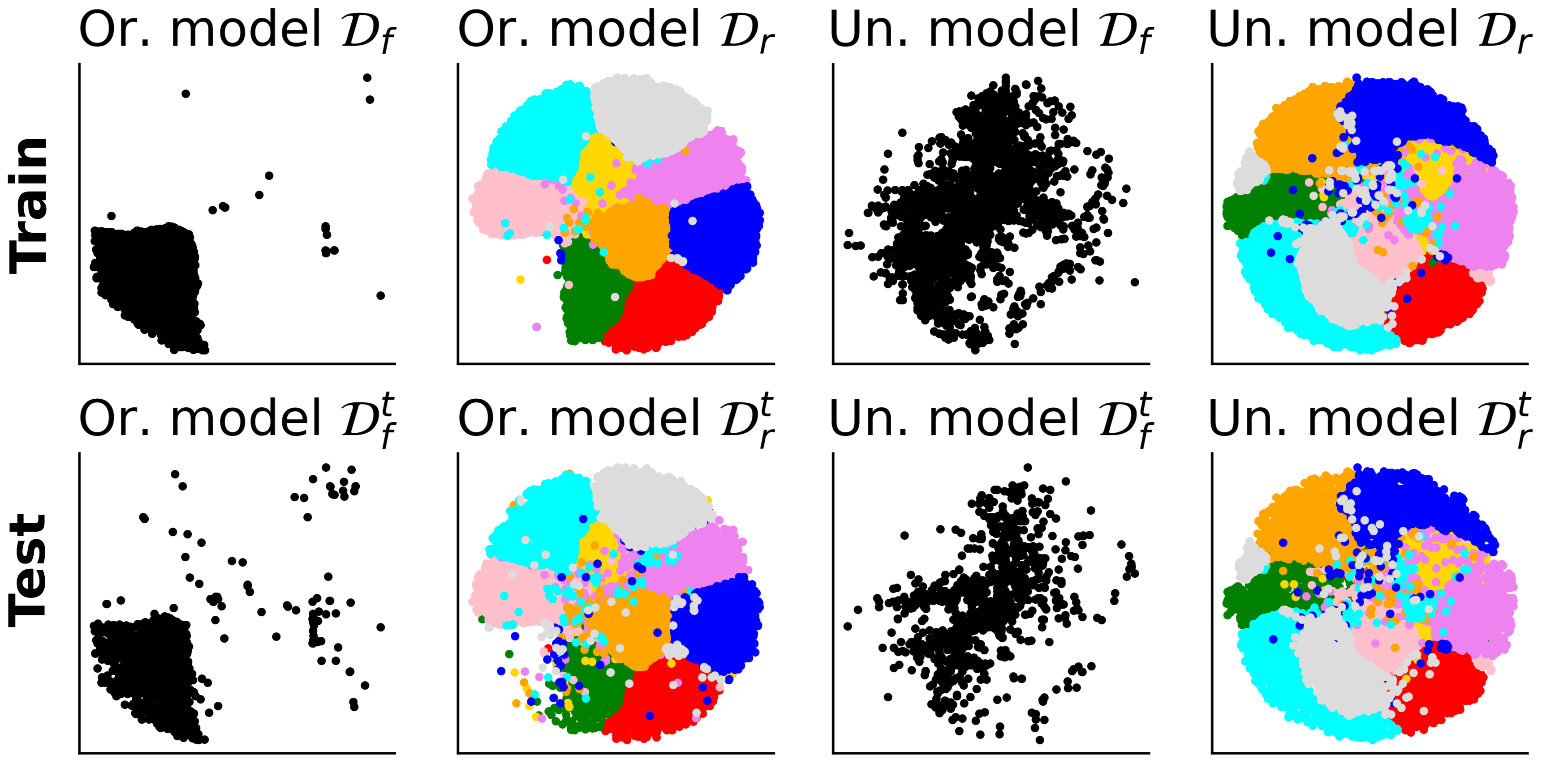
Figure 2: Visualization of $\mathcal{D}_{r}$, $\mathcal{D}_{f}$, $\mathcal{D}_{r}^{t}$ and $\mathcal{D}_{f}^{t}$ samples embeddings obtained using TSNE[43] of CIFAR-10 dataset for CR scenario. Embeddings are represented for the original model (Or. model) and the unlearned model (Un. model). Black dots represent the target class that has to be removed. The solid dots in different colors represent samples belonging to different remaining classes. Ideally, forgetting samples are scattered between all the remaining classes.

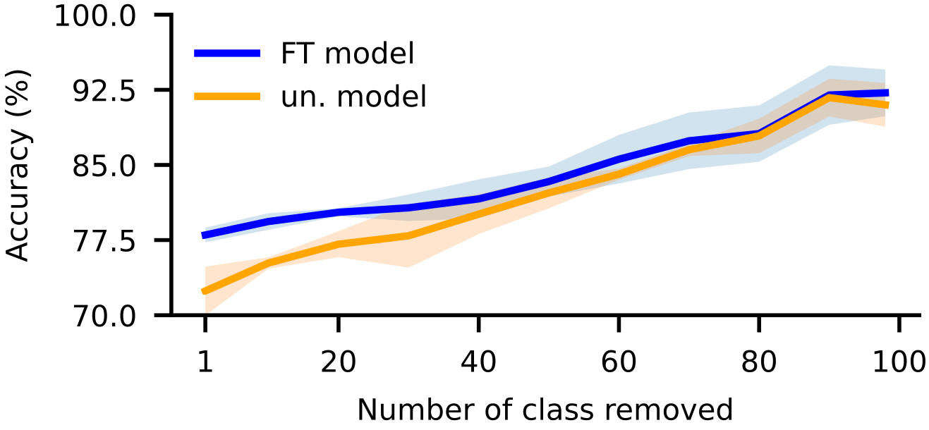
Figure 3: DUCK accuracy performance on $\mathcal{D}_{r}^{t}$ of CIFAR100 (orange) in comparison with the model finetuned on $\mathcal{D}_{r}$ (blue) as a function of the number of classes removed. The accuracy and std reported are mean computed over 10 different shufflings of the classes.

4.5 Manifold Analysis

To better understand the effect of the unlearning mechanism of our method, we analyzed the embeddings extracted from the backbone of the neural network ($\Psi_{\theta}$) both before and after the unlearning process in the CR scenario. In Figure 2, we report the application of t-SNE [43] to the extracted embeddings, with each class represented by a distinct color cluster. We fit 2 different t-SNEs respectively for the original model and the unlearned model embeddings. Prior to the application of DUCK (the first two columns in the figure), embeddings corresponding to different classes are clearly clustered together in both the train and test sets. Following the application of DUCK, while the embeddings of the retain-set samples are still clustered together, the embeddings of the forget-set are scattered across all the other classes clusters. The results suggest how the information content of the embeddings of the forget-set extracted from $\Psi_{\theta}$ is no longer reliable and useful for the classification of these samples.

4.6 Multiple Class-Removal Scenario

In addition to CR and HR scenarios, we opted to assess the performance of our algorithm when multiple classes are removed from the dataset. This scenario represents an extension of CR, where target accuracies for the removed classes are 0 likewise. In Figure 3, we present the results in terms of accuracy on the retained test set while varying the number of classes to be removed. Remarkably, DUCK achieves high test accuracy even with a large number of classes in the forget-set. Furthermore, it demonstrates performance comparable to the more resource-intensive Finetuning method.

4.7 Unlearning Time Analysis

As a further analysis, we plot in Figure 4 the retain test accuracy and AUS as a function of the unlearning time for all the methods considered in the CR scenario. Notably, DUCK is consistently superior in terms of both scores, surpassed only by Finetuning, which is $\sim$2 order of magnitude slower. The only faster method is Negative Gradient, at the cost of a lower performance in the other metrics. From these results, it is possible to evince that DUCK is an effective method able to balance the time-accuracy tradeoff. Furthermore, in Sec F, we present a similar plot for the HR scenario, where the superiority of DUCK is even more pronounced.

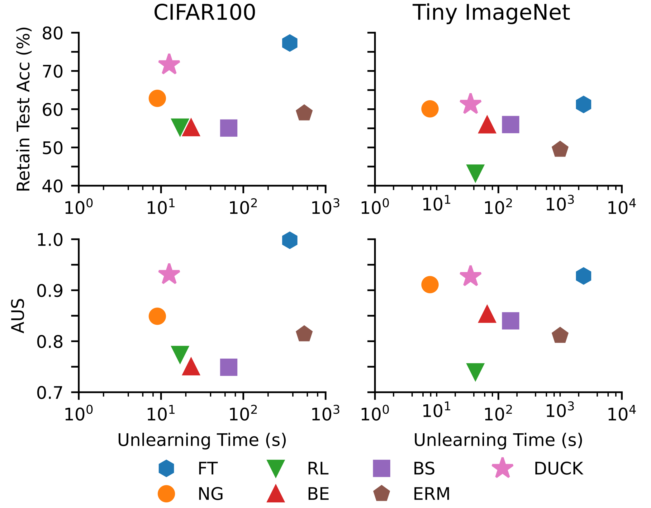
Figure 4: DUCK outperforms state-of-the-art unlearning algorithms in CR scenario. Average test accuracy in the class-removal scenario for retain-set $\mathcal{D}^{t}_{r}$ and AUS as a function of the unlearning time for CIFAR-100 and TinyImagenet. Accuracies and AUS are reported as mean across 10 runs where for each one a different target class was selected.

4.8 Architectural Analaysis

To assess the method’s robustness concerning changes in the model architecture, we conducted experiments using various backbone architectures, specifically AllCNN, resnet18, resnet34, and resnet50 models. These models are listed in ascending order based on the number of parameters. The results regarding accuracy and AUS are detailed in Table 4. Observing the outcomes, we note that as the model size increases, the AUS also increases. This trend is evident as the gap between the original and unlearned retain test accuracy decreases. We hypothesize that this occurrence is due to the larger number of weights available, leading to fewer weights shared for representing each class. Consequently, the impact of forgetting on retain test samples decreases with larger model architectures. Overall, DUCK represents a valid model-agnostic solution to machine unlearning problems. We report in Sec G the results of the architectural analysis in the CR scenario for the TinyImagenet.

Table 4: Comparison between the results of the application of our method to several pre-trained neural architectures in CIFAR100 on the CR scenario. The accuracies reported here are the mean accuracies computed over 10 runs where for each one a different class has to be forgotten.

		$\mathcal{A}_{r}$	$\mathcal{A}_{f}$	$\mathcal{A}^{t}_{r}$	$\mathcal{A}^{t}_{f}$	AUS
AllCNN	Original	99.77	99.72	69.70	70.83	0.585
	Unlearned	88.66	00.32	61.36	00.50	0.912
Resnet18	Original	99.63	99.70	77.55	77.50	0.563
	Unlearned	92.56	00.34	71.57	01.00	0.931
Resnet34	Original	99.98	99.98	80.30	80.13	0.555
	Unlearned	99.84	00.00	75.59	00.00	0.953
Resnet50	Original	99.98	99.93	80.80	80.62	0.553
	Unlearned	98.69	00.58	77.00	00.70	0.955

5 Conclusions

In this paper, we introduce DUCK, a novel unlearning algorithm based on metric learning. DUCK exhibits versatility by operating effectively in diverse scenarios such as CR and HR, addressing heterogeneous unlearning tasks. Our algorithm outperforms several state-of-the-art methods. It is also comparable with upper-bound methods like Retraining and Finetuning while being more efficient in terms of speed. We also present a novel MIA specifically designed for the HR scenario. This MIA assesses whether information about the membership of forget-data is preserved. The results achieved by MIA, across the various datasets, confirm the ability of DUCK to unlearn a random subset of training data without information leakage. Overall, DUCK is a consistent, computationally efficient, model-agnostic, and verifiable unlearning method.
DUCK opens avenues for the development of end-to-end strategies to detect model poisoning attacks through adversarial data [22, 36, 41] and restore model capabilities. Additionally, given the increasing prevalence of multi-modal models [21, 31, 29, 32], there is a need for an extension of the unlearning algorithm beyond the scope of pure computer vision. Therefore, the development of a multi-modal version of DUCK holds significant importance.

Supplementary Material

Appendix A Datasets Details

This section provides detailed information about the four publicly available datasets utilized in the experiments outlined in Sec 4: CIFAR10[17], CIFAR100[17], TinyImagenet[19], and VGGFace2[3].

CIFAR10 and CIFAR100.   Both datasets consist of 60,000 images sized $32\times 32$, split into a training set of 50,000 images and a test set of 10,000 images. CIFAR10 contains 10 classes, with 6,000 samples for each class, while CIFAR100 includes 100 classes, resulting in 600 images per class.

TinyImagenet.   Resized from the larger ImageNet dataset[9], TinyImagenet comprises 110,000 images sized $64\times 64$, distributed across 200 classes. The training set contains 100,000 images (500 per class), and the test set contains 10,000 images (50 per class), following a structure similar to CIFAR100.

VGGFace2.   VGGFace2 comprises 3.31 million images sized $128\times 128$ belonging to 9,131 subjects, with an average of 362.6 images per subject. The dataset is split into training and test sets, with the training set containing images from 8,631 subjects and the test set containing 500 identities. For consistency with [11], we retained only the top 10 subjects from the original training set, each having the highest number of images. The final dataset dimensions are 7380, with 738$\pm$50 images for each subject. This reduced dataset version is further divided into an 80$\%$ training set and a 20$\%$ test set.

Appendix B Experimental Details

In this Section, we report the experimental details for the training and evaluation of DUCK and all the considered methods.

DUCK Hyperparameters and setting.   In Table 5, we present the hyperparameters employed in DUCK for all the considered scenarios. The upper section of the table pertains to the class-removal scenario (CR), while the lower section refers to the Homogeneous-Removal (HR) scenario. The Temperature parameter is utilized to scale probabilities in the computation of the cross-entropy loss (Eq. 4).

Due to the dataset limited dimensions, experiments in the HR scenario were not conducted for the VGGFace2 dataset. For the multiple class removal experiment, which represents a challenging variant of the CR scenario, we maintained fixed hyperparameters while reducing the batch ratio to 1 when at least 50 classes are removed.

Table 5: Hyperparameters employed in DUCK for both the CR and HR scenarios. Experiments in the HR scenario were not conducted for the VGGFace2 dataset due to its limited dimensions.

		CIFAR10	CIFAR100	TinyImagenet	VGGFace2
CR	$\lambda_{\text{fgt}}$	1.5	1.5	0.5	1.5
	$\lambda_{\text{ret}}$	1.5	1.5	1.5	1.5
	Batch Ratio	5	5	30	1
	Learning Rate	$1\text{\times}{10}^{-3}$	$1\text{\times}{10}^{-3}$	$2\text{\times}{10}^{-4}$	$1\text{\times}{10}^{-3}$
	Batch Size	1024	1024	1024	128
	Temperature	2	2	3	1
HR	$\lambda_{\text{fgt}}$	1	1	1.5	-
	$\lambda_{\text{ret}}$	1.4	1.4	1.5	-
	Batch Ratio	5	5	5	-
	Learning Rate	$1\text{\times}{10}^{-3}$	$1\text{\times}{10}^{-3}$	$5\text{\times}{10}^{-4}$	-
	Batch Size	1024	1024	1024	-
	Temperature	2	2	3	-

Baselines and competitors hyperparameters and settings.   In Table 6 and Table 7, we outline the hyperparameters utilized in conducting experiments with the baselines (Original, Retrained, and FineTuning) and the considered competitor methods (Random Labels, Negative Gradient, Boundary Shrink, Boundary Expanding, and ERM-KTP).

As specified in Sec 4, we solely executed the HR scenario for the methods capable of supporting this setting. Notably, for Random Labels and Negative Gradient, the number of epochs is denoted as $\star$. This signifies that, in these experiments, they were executed for an unspecified number of epochs, continuing until they met the same stopping criteria as DUCK ($A^{\star}_{f}=0.01$ for CR and $A^{\star}_{f}=A^{\text{Or}}_{t}$ for HR). The symbol $-$ indicates that the learning rate scheduler was not utilized.

Table 6: Hyperparameters utilized for experiments with baselines (Original, Retrained, and FineTuning) and the considered competitors (Random Labels, Negative Gradient, Boundary Shrink, Boundary Expanding, and ERM-KTP) in the class-removal (CR) scenario. For Random Labels and Negative Gradient, the number of epochs denoted by $\star$ indicates the experiments ran until meeting the stopping criteria akin to DUCK ($A^{\star}_{f}=0.01$ for CR). The symbol $-$ signifies that the learning rate scheduler was not employed.

		Original	Retrained	FineTuning	Random Labels	Negative Gradient	Boundary Shrink	Boundary Expanding	ERM-KTP
CIFAR10	Learning Rate	$1\text{\times}{10}^{-1}$	$1\text{\times}{10}^{-1}$	$1\text{\times}{10}^{-1}$	$1\text{\times}{10}^{-3}$	$1\text{\times}{10}^{-2}$	$1\text{\times}{10}^{-5}$	$1\text{\times}{10}^{-5}$	$1\text{\times}{10}^{-1}$
	Batch Size	256	256	32	256	256	64	64	256
	Epochs	300	300	30	$\star$	$\star$	15	10	50
	Scheduler	Cosine-Annealing	Cosine-Annealing	[8, 15]	[3]	-	-	-	[10,20] $\gamma=0.1$
CIFAR100	Learning Rate	$1\text{\times}{10}^{-1}$	$1\text{\times}{10}^{-1}$	$1\text{\times}{10}^{-1}$	$1\text{\times}{10}^{-2}$	$1\text{\times}{10}^{-2}$	$1\text{\times}{10}^{-5}$	$1\text{\times}{10}^{-5}$	$1\text{\times}{10}^{-1}$
	Batch Size	256	256	32	256	256	64	64	256
	Epochs	300	300	30	$\star$	$\star$	15	10	50
	Scheduler	Cosine-Annealing	Cosine-Annealing	[8, 15]	-	-	-	-	[10,20] $\gamma=0.1$
Tiny Imagenet	Learning Rate	$1\text{\times}{10}^{-1}$	$1\text{\times}{10}^{-1}$	$1\text{\times}{10}^{-1}$	$2.5\text{\times}{10}^{-3}$	$1\text{\times}{10}^{-2}$	$1\text{\times}{10}^{-5}$	$1\text{\times}{10}^{-5}$	$1\text{\times}{10}^{-1}$
	Batch Size	256	256	32	256	256	64	64	256
	Epochs	300	300	30	$\star$	$\star$	15	10	50
	Scheduler	[every 25] $\gamma=0.1$	[every 25] $\gamma=0.1$	[8, 15]	-	-	-	-	[10,20] $\gamma=0.1$
VGGFace2	Learning Rate	$5\text{\times}{10}^{-4}$	$5\text{\times}{10}^{-4}$	$1\text{\times}{10}^{-1}$	$1\text{\times}{10}^{-3}$	$1\text{\times}{10}^{-2}$	$1\text{\times}{10}^{-5}$	$1\text{\times}{10}^{-5}$	$1\text{\times}{10}^{-1}$
	Batch Size	128	128	32	256	64	64	64	256
	Epochs	14	14	30	$\star$	$\star$	15	10	100
	Scheduler	-	-	-	[6]	-	-	-	[50,80] $\gamma=0.1$

Table 7: Hyperparameters used for experiments with baselines (Original, Retrained, and FineTuning) and supported competitors in the Homogeneous-Removal (HR) scenario. The HR experiments were conducted for methods compatible with this setting. For Random Labels and Negative Gradient, the $\star$ symbol implies that the experiments were executed until reaching the same stopping criteria as DUCK ($A^{\star}_{f}=A^{\text{Or}}_{t}$ for HR). The presence of $-$ denotes that the learning rate scheduler was not employed.

		Original	Retrained	FineTuning	Random Labels	Negative Gradient
CIFAR10	Learning Rate	$1\text{\times}{10}^{-1}$	$1\text{\times}{10}^{-1}$	$1\text{\times}{10}^{-1}$	$1\text{\times}{10}^{-4}$	$3\text{\times}{10}^{-4}$
	Batch Size	256	256	32	256	256
	Epochs	300	300	30	$\star$	$\star$
	Scheduler	Cosine-Annealing	Cosine-Annealing	[8, 15]	[5]	[4]
CIFAR100	Learning Rate	$1\text{\times}{10}^{-1}$	$1\text{\times}{10}^{-1}$	$1\text{\times}{10}^{-1}$	$1.2\text{\times}{10}^{-3}$	$4\text{\times}{10}^{-4}$
	Batch Size	256	256	32	256	256
	Epochs	300	300	30	$\star$	$\star$
	Scheduler	Cosine-Annealing	Cosine-Annealing	[8, 15]	[9]	[7,9]
Tiny Imagenet	Learning Rate	$1\text{\times}{10}^{-1}$	$1\text{\times}{10}^{-1}$	$1\text{\times}{10}^{-1}$	$1\text{\times}{10}^{-3}$	$6\text{\times}{10}^{-5}$
	Batch Size	256	256	32	256	256
	Epochs	300	300	30	$\star$	$\star$
	Scheduler	[every 25] $\gamma=0.1$	[every 25] $\gamma=0.1$	[8, 15]	[7]	[5, 12]

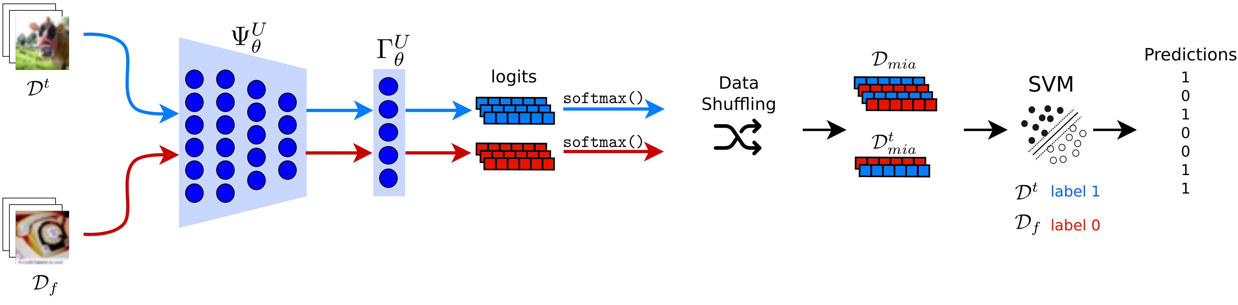
Figure 5: Architecture scheme representing the Membership Inference Attack (MIA). The logits vectors of datasets $\mathcal{D}_{f}$ (forget-set) and $\mathcal{D}^{t}$ (test-set) are combined, shuffled, and split into a training set $\mathcal{D}_{\text{mia}}$ (80% of samples), and a test set $\mathcal{D}_{\text{mia}}^{t}$ (20% of samples). An SVM with a Gaussian kernel classifier is then trained to distinguish between $\mathcal{D}_{f}$ and $\mathcal{D}^{t}$ instances.

Code Execution Details.   In this section we report the experimental details for reproducing the experiments of Sec 4. We first trained the Original models for the four considered datasets using the seed 42.

For the CR scenario, for all the datasets considered, and all the unlearning methods, the experimental steps were:

1. Fix the seed to 42.

2. Split the dataset in retain (train/test) and forget (train/test) composed by all the instances of a class $i$.

3. Run the unlearning.

4. Evaluate the unlearned model on the retain (train/test) and forget (train/test) sets.

5. Repeat stpes (2)-(4) selecting a different class $i$.

6. Compute metrics averaging on the indices $i$ representing the classes removed at each iteration.

In this scenario, for CIFAR10 and VGGFace2, each iteration utilized one of the ten classes as the forget set. For CIFAR100 and TinyImagenet, the forget-set included classes that were multiples of 10 and 20 starting from 0 (e.g., CIFAR100: 0, 10, 20, …, 90; TinyImagenet: 0, 20, 40, …, 180).

For the HR scenario, for all the datasets considered, and all the methods, the experimental steps were:

1. Fix the seed $i$

2. Generate the forget set randomly picking 10% of the images from the original training dataset. Generate the retain-set with the remaining 90%

3. Run the unlearning.

4. Evaluate the unlearned model on the retain, forget, and test sets.

5. Repeat stpes (1)-(4) selecting a different seed $i$.

6. Compute metrics averaging on the indices $i$ representing the seeds.

The experiments were conducted using the following seeds: $\left[0,1,2,3,4,5,6,7,8,42\right]$.

These experimental protocols were consistently applied across all experiments presented in the paper, encompassing ablation studies, multiple class removal scenario, time analysis, and architectural analysis. The code we used for the experiments of the paper can be found at https://github.com/OcraM17/DUCK

Appendix C AUS in depth

Each forgetting algorithm aims to increase the AUS score by optimizing two compelling objectives: preserving a high $\mathcal{A}_{t}$ on the retained classes and erasing all the information relative to the forget-set. The AUS encompasses the balance between the effectiveness of forgetting and the capability of the model to retain information. A baseline value for each dataset is represented by the AUS of its corresponding original model AUS^Or: since $\mathcal{A}_{t}=\mathcal{A}^{Or}_{t}$ ($i.e.$ numerator =1), AUS^Or exists in the range $[0.5,1]$. Provided that the original model is well trained and not excessively overfitted, AUS^Or is typically low and close to 0.5 in CR ($\mathcal{A}_{f}^{Or}\simeq\mathcal{A}_{r}^{Or}\gg 0$), while higher in HR (where $\Delta$ is proportional to the model’s degree of overfitting and is expected not to be excessively large).

An AUS lower than the AUS^Or signals an anomaly, often suggesting that the forgetting algorithm is ill-suited for the scenario. It indicates that the forgetting on the test retain-set is comparable to or greater than the forgetting on the forget-set. On the other hand, as there is no absolute value in the numerator, an AUS greater than $1$ is also possible: implying that post-forgetting, the model’s accuracy on the test retain-set has improved. This could occur due to two reasons:

• The result is a fluctuation, and repeating the experiment should give numbers compatible with 1.

• The original model might not have been adequately trained, and during the forgetting process, the model could extract information from data previously disregarded or underutilized.

Appendix D MIA Additional Details

During the MIA, the hyperparameters of the SVM with gaussian kernel were tuned through a grid search using a 3-fold cross-validation strategy. The objective of this procedure was to identify the best and most reliable hyperparameters of the SVM classifier, resulting in the best classification accuracy of retain and forget samples. The varied hyperparameters include the regularization parameter $C$, which takes values in the set $\left[1,5,10,100\right]$, and the kernel coefficient $\gamma$, which takes values in the set $\left[1,0.1,0.01\right]$. In order to better clarify the working mechanism of the Membership Inference Attack defined in Sec 4.3 , we report the scheme in Figure 5.

Appendix E Additional Ablation Study

Table 8: Results of the ablation study conducted on the CIFAR100 and TinyImagenet datasets within the CR scenario. The metrics reported herein represent the mean values obtained over 10 independent runs, with each run employing a different forget class setting.

	$\mathcal{L}_{\text{FGT}}$	$\mathcal{L}_{\text{RET}}$	$\mathcal{A}_{r}$	$\mathcal{A}_{f}$	$\mathcal{A}_{r}^{t}$	$\mathcal{A}_{f}^{t}$	Un. Time[s]
CIFAR100	✗	✗	99.63	99.70	77.55	77.50	-
	✓	✗	67.92	00.04	51.52	00.70	11.56
	✗	✓	91.51	00.32	72.05	00.40	19.06
	✓	✓	92.56	00.34	71.57	01.00	12.32
Tiny	✗	✗	84.92	84.62	68.26	64.60	-
	✓	✗	31.15	00.22	25.81	01.40	225.42
	✗	✓	75.55	00.67	61.25	01.33	261.21
	✓	✓	72.10	00.06	61.29	00.20	98.25

In Table 8, we present a parallel investigation conducted in the CR scenario, mirroring the analysis provided in Table 3 for the HR scenario. We conducted an ablation study on CIFAR100 and TinyImagenet, selectively deactivating either $\mathcal{L}_{\text{RET}}$ or $\mathcal{L}_{\text{FGT}}$ while keeping the remaining hyperparameters constant. In the first row of the table, the results of the Original model are presented. When $\mathcal{L}_{\text{RET}}$ is absent, there is a reduction in test accuracy performance in both CIFAR100 and TinyImagenet, although smaller in comparison to the HR scenario. On the other hand, setting $\mathcal{L}{\text{FGT}}$ to 0 implies the unlearning strategy reduces to tuning the original model on the retain-set using a stopping mechanism based on the accuracy of the forget-set. As expected, the performance observed for this setting is close to the model unlearned using DUCK, albeit at the cost of almost doubling the training time.

Appendix F Additional Time Analysis

In Figure 6 we report the test accuracy and AUS score as a function of the unlearning time in the HR scenario for CIFAR100 and TinyImagenet dataset. The results reported confirm once more how DUCK outperforms all other state-of-the-art methods and is at the same time comparable in terms of accuracy or AUS performance but much faster than Finetuning.

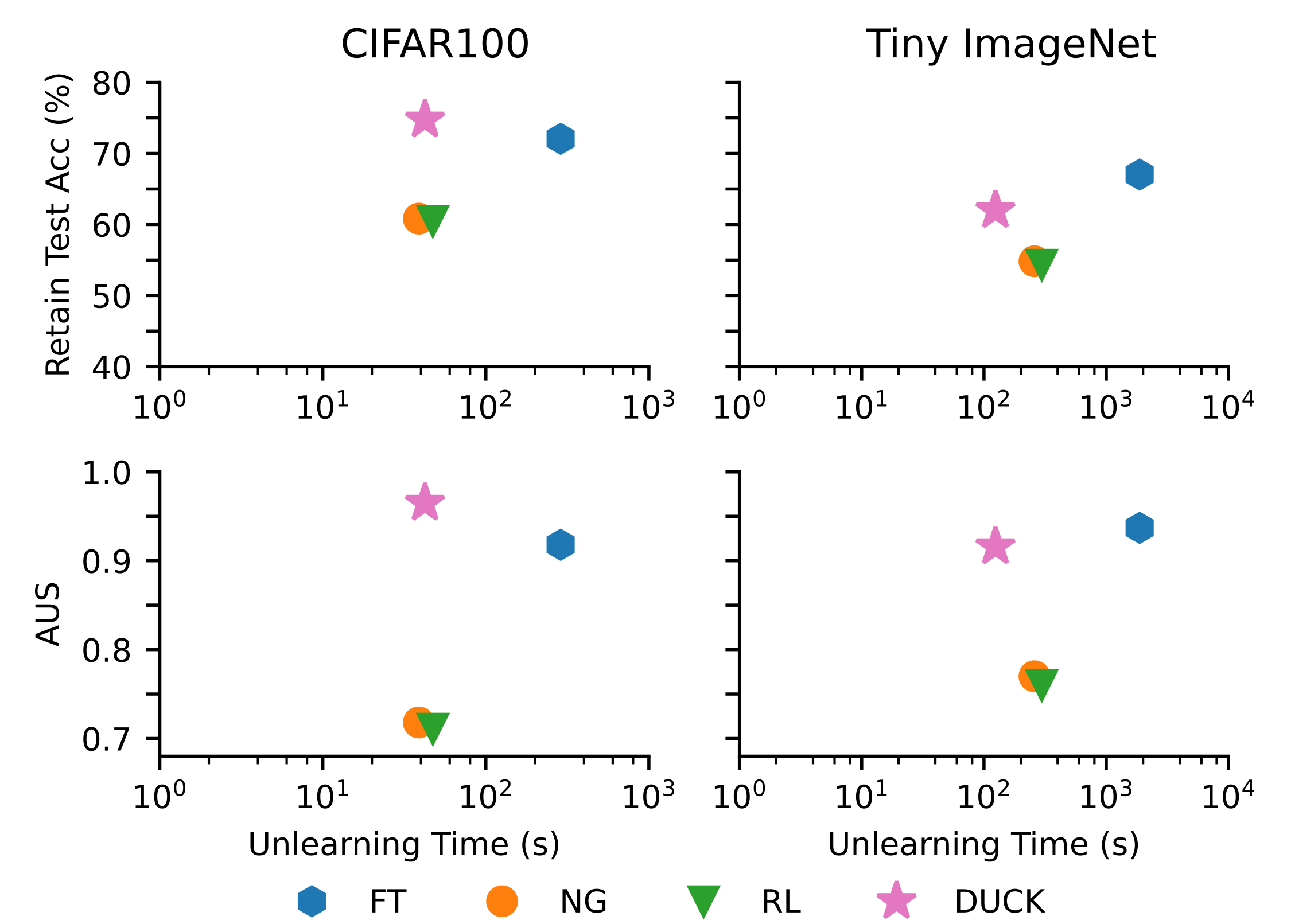
Figure 6: Unlearning time comparison in the HR scenario. Average test accuracy $\mathcal{D}^{t}$ and AUS as a function of the unlearning time for CIFAR-100 and TinyImagenet. Accuracies and AUS are reported as mean across 10 runs where for each one a different seed and forget split was selected.

Appendix G Additional Architectural Analysis

Table 9: Comparison between the results of the application of DUCK to several pre-trained neural architectures on TinyImagenet in the CR scenario. We report the mean accuracies computed over 10 runs where for each one a different class has to be forgotten.

	TinyImagenet
		$\mathcal{A}_{r}$	$\mathcal{A}_{f}$	$\mathcal{A}_{r}^{t}$	$\mathcal{A}_{f}^{t}$	AUS
AllCNN	Original	69.91	66.82	52.79	50.40	0.665
	Unlearned	57.28	00.60	45.78	00.40	0.926
Resnet18	Original	84.92	84.62	68.26	64.60	0.607
	Unlearned	72.10	00.06	61.29	00.20	0.927
Resnet34	Original	93.60	93.66	70.21	72.00	0.581
	Unlearned	79.68	00.08	64.09	00.20	0.937
Resnet50	Original	91.01	90.90	75.37	77.40	0.564
	Unlearned	82.10	00.02	69.61	00.00	0.942

Similarly to Table 4, we present the comparison of the results obtained using different backbone architectures on the TinyImagenet dataset (Table 9) confirming the results obtained in CIFAR100. Overall, these results underline how DUCK can be considered an effective model-agnostic unlearning approach.

References

- Boulemtafes et al. [2020] Amine Boulemtafes, Abdelouahid Derhab, and Yacine Challal. A review of privacy-preserving techniques for deep learning. Neurocomputing, 384:21–45, 2020.
- Bourtoule et al. [2021] Lucas Bourtoule, Varun Chandrasekaran, Christopher A Choquette-Choo, Hengrui Jia, Adelin Travers, Baiwu Zhang, David Lie, and Nicolas Papernot. Machine unlearning. In 2021 IEEE Symposium on Security and Privacy (SP), pages 141–159. IEEE, 2021.
- Cao et al. [2018] Qiong Cao, Li Shen, Weidi Xie, Omkar M Parkhi, and Andrew Zisserman. Vggface2: A dataset for recognising faces across pose and age. In 2018 13th IEEE international conference on automatic face & gesture recognition (FG 2018), pages 67–74. IEEE, 2018.
- Cao and Yang [2015] Yinzhi Cao and Junfeng Yang. Towards making systems forget with machine unlearning. In 2015 IEEE symposium on security and privacy, pages 463–480. IEEE, 2015.
- Carlini et al. [2022] Nicholas Carlini, Steve Chien, Milad Nasr, Shuang Song, Andreas Terzis, and Florian Tramèr. Membership inference attacks from first principles. In 43rd IEEE Symposium on Security and Privacy, SP 2022, San Francisco, CA, USA, May 22-26, 2022, pages 1897–1914. IEEE, 2022.
- Chen et al. [2021] Min Chen, Zhikun Zhang, Tianhao Wang, Michael Backes, Mathias Humbert, and Yang Zhang. When machine unlearning jeopardizes privacy. In Proceedings of the 2021 ACM SIGSAC conference on computer and communications security, pages 896–911, 2021.
- Chen et al. [2023] Min Chen, Weizhuo Gao, Gaoyang Liu, Kai Peng, and Chen Wang. Boundary unlearning: Rapid forgetting of deep networks via shifting the decision boundary. In Proceedings of the IEEE/CVF Conference on Computer Vision and Pattern Recognition, pages 7766–7775, 2023.
- Chundawat et al. [2023] Vikram S Chundawat, Ayush K Tarun, Murari Mandal, and Mohan Kankanhalli. Zero-shot machine unlearning. IEEE Transactions on Information Forensics and Security, 2023.
- Deng et al. [2009] Jia Deng, Wei Dong, Richard Socher, Li-Jia Li, Kai Li, and Li Fei-Fei. Imagenet: A large-scale hierarchical image database. In 2009 IEEE conference on computer vision and pattern recognition, pages 248–255. Ieee, 2009.
- Fu et al. [2022] Shaopeng Fu, Fengxiang He, and Dacheng Tao. Knowledge removal in sampling-based bayesian inference. arXiv preprint arXiv:2203.12964, 2022.
- Golatkar et al. [2020] Aditya Golatkar, Alessandro Achille, and Stefano Soatto. Eternal sunshine of the spotless net: Selective forgetting in deep networks. In Proceedings of the IEEE/CVF Conference on Computer Vision and Pattern Recognition, pages 9304–9312, 2020.
- Graves et al. [2021] Laura Graves, Vineel Nagisetty, and Vijay Ganesh. Amnesiac machine learning. In Proceedings of the AAAI Conference on Artificial Intelligence, pages 11516–11524, 2021.
- Gupta et al. [2021] Varun Gupta, Christopher Jung, Seth Neel, Aaron Roth, Saeed Sharifi-Malvajerdi, and Chris Waites. Adaptive machine unlearning. Advances in Neural Information Processing Systems, 34:16319–16330, 2021.
- Hayase et al. [2020] Tomohiro Hayase, Suguru Yasutomi, and Takashi Katoh. Selective forgetting of deep networks at a finer level than samples. arXiv preprint arXiv:2012.11849, 2020.
- Hu et al. [2022] Hongsheng Hu, Zoran Salcic, Lichao Sun, Gillian Dobbie, Philip S Yu, and Xuyun Zhang. Membership inference attacks on machine learning: A survey. ACM Computing Surveys (CSUR), 54(11s):1–37, 2022.
- Kim and Woo [2022] Junyaup Kim and Simon S Woo. Efficient two-stage model retraining for machine unlearning. In Proceedings of the IEEE/CVF Conference on Computer Vision and Pattern Recognition, pages 4361–4369, 2022.
- Krizhevsky et al. [2009] Alex Krizhevsky, Geoffrey Hinton, et al. Learning multiple layers of features from tiny images. 2009.
- Kurmanji et al. [2023] Meghdad Kurmanji, Peter Triantafillou, and Eleni Triantafillou. Towards unbounded machine unlearning. arXiv preprint arXiv:2302.09880, 2023.
- Le and Yang [2015] Ya Le and Xuan S. Yang. Tiny imagenet visual recognition challenge. 2015.
- Lin et al. [2023] Shen Lin, Xiaoyu Zhang, Chenyang Chen, Xiaofeng Chen, and Willy Susilo. Erm-ktp: Knowledge-level machine unlearning via knowledge transfer. In Proceedings of the IEEE/CVF Conference on Computer Vision and Pattern Recognition, pages 20147–20155, 2023.
- Liu et al. [2023a] Haotian Liu, Chunyuan Li, Qingyang Wu, and Yong Jae Lee. Visual instruction tuning, 2023a.
- Liu et al. [2023b] Junxu Liu, Mingsheng Xue, Jian Lou, Xiaoyu Zhang, Li Xiong, and Zhan Qin. Muter: Machine unlearning on adversarially trained models. In Proceedings of the IEEE/CVF International Conference on Computer Vision, pages 4892–4902, 2023b.
- Loshchilov and Hutter [2017] Ilya Loshchilov and Frank Hutter. Decoupled weight decay regularization. arXiv preprint arXiv:1711.05101, 2017.
- Magdziarczyk [2019] Malgorzata Magdziarczyk. Right to be forgotten in light of regulation (eu) 2016/679 of the european parliament and of the council of 27 april 2016 on the protection of natural persons with regard to the processing of personal data and on the free movement of such data, and repealing directive 95/46/ec. In 6th International Multidisciplinary Scientific Conference on Social Sciences and Art Sgem 2019, pages 177–184, 2019.
- Marchant et al. [2022] Neil G Marchant, Benjamin IP Rubinstein, and Scott Alfeld. Hard to forget: Poisoning attacks on certified machine unlearning. In Proceedings of the AAAI Conference on Artificial Intelligence, pages 7691–7700, 2022.
- Mehta et al. [2022] Ronak Mehta, Sourav Pal, Vikas Singh, and Sathya N Ravi. Deep unlearning via randomized conditionally independent hessians. In Proceedings of the IEEE/CVF Conference on Computer Vision and Pattern Recognition, pages 10422–10431, 2022.
- Mercuri et al. [2022] Salvatore Mercuri, Raad Khraishi, Ramin Okhrati, Devesh Batra, Conor Hamill, Taha Ghasempour, and Andrew Nowlan. An introduction to machine unlearning. arXiv preprint arXiv:2209.00939, 2022.
- Nguyen et al. [2022] Thanh Tam Nguyen, Thanh Trung Huynh, Phi Le Nguyen, Alan Wee-Chung Liew, Hongzhi Yin, and Quoc Viet Hung Nguyen. A survey of machine unlearning. arXiv preprint arXiv:2209.02299, 2022.
- OpenAI [2023] OpenAI. Gpt-4 technical report, 2023.
- Pardau [2018] Stuart L Pardau. The california consumer privacy act: Towards a european-style privacy regime in the united states. J. Tech. L. & Pol’y, 23:68, 2018.
- Radford et al. [2021] Alec Radford, Jong Wook Kim, Chris Hallacy, Aditya Ramesh, Gabriel Goh, Sandhini Agarwal, Girish Sastry, Amanda Askell, Pamela Mishkin, Jack Clark, et al. Learning transferable visual models from natural language supervision. In International conference on machine learning, pages 8748–8763. PMLR, 2021.
- Ramesh et al. [2022] Aditya Ramesh, Prafulla Dhariwal, Alex Nichol, Casey Chu, and Mark Chen. Hierarchical text-conditional image generation with clip latents. arXiv preprint arXiv:2204.06125, 1(2):3, 2022.
- Ramkumar et al. [2023] Vijaya Raghavan T Ramkumar, Elahe Arani, and Bahram Zonooz. Learn, unlearn and relearn: An online learning paradigm for deep neural networks. arXiv preprint arXiv:2303.10455, 2023.
- Ren et al. [2020] Kui Ren, Tianhang Zheng, Zhan Qin, and Xue Liu. Adversarial attacks and defenses in deep learning. Engineering, 6(3):346–360, 2020.
- Salem et al. [2019] Ahmed Salem, Yang Zhang, Mathias Humbert, Pascal Berrang, Mario Fritz, and Michael Backes. Ml-leaks: Model and data independent membership inference attacks and defenses on machine learning models. In 26th Annual Network and Distributed System Security Symposium, NDSS. The Internet Society, 2019.
- Setlur et al. [2022] Amrith Setlur, Benjamin Eysenbach, Virginia Smith, and Sergey Levine. Adversarial unlearning: Reducing confidence along adversarial directions. Advances in Neural Information Processing Systems, 35:18556–18570, 2022.
- Shaik et al. [2023] Thanveer Basha Shaik, Xiaohui Tao, Haoran Xie, Lin Li, Xiaofeng Zhu, and Qing Li. Exploring the landscape of machine unlearning: A comprehensive survey and taxonomy. CoRR, 2023.
- Shokri and Shmatikov [2015] Reza Shokri and Vitaly Shmatikov. Privacy-preserving deep learning. In Proceedings of the 22nd ACM SIGSAC conference on computer and communications security, pages 1310–1321, 2015.
- Shokri et al. [2017] Reza Shokri, Marco Stronati, Congzheng Song, and Vitaly Shmatikov. Membership inference attacks against machine learning models. In IEEE Symposium on Security and Privacy, SP. IEEE Computer Society, 2017.
- Song et al. [2019] Liwei Song, Reza Shokri, and Prateek Mittal. Privacy risks of securing machine learning models against adversarial examples. In Conference on Computer and Communications Security, CCS. ACM, 2019.
- Sun et al. [2023] Hui Sun, Tianqing Zhu, Wenhan Chang, and Wanlei Zhou. Generative adversarial networks unlearning. arXiv preprint arXiv:2308.09881, 2023.
- Tarun et al. [2023] Ayush K Tarun, Vikram S Chundawat, Murari Mandal, and Mohan Kankanhalli. Fast yet effective machine unlearning. IEEE Transactions on Neural Networks and Learning Systems, 2023.
- Van der Maaten and Hinton [2008] Laurens Van der Maaten and Geoffrey Hinton. Visualizing data using t-sne. Journal of machine learning research, 9(11), 2008.
- Villaronga et al. [2018] Eduard Fosch Villaronga, Peter Kieseberg, and Tiffany Li. Humans forget, machines remember: Artificial intelligence and the right to be forgotten. Computer Law & Security Review, 34(2):304–313, 2018.
- Xu et al. [2023] Jie Xu, Zihan Wu, Cong Wang, and Xiaohua Jia. Machine unlearning: Solutions and challenges. arXiv preprint arXiv:2308.07061, 2023.
- Yan et al. [2022] Haonan Yan, Xiaoguang Li, Ziyao Guo, Hui Li, Fenghua Li, and Xiaodong Lin. Arcane: An efficient architecture for exact machine unlearning. In Proceedings of the Thirty-First International Joint Conference on Artificial Intelligence, IJCAI-22, pages 4006–4013, 2022.
- Yeom et al. [2018] Samuel Yeom, Irene Giacomelli, Matt Fredrikson, and Somesh Jha. Privacy risk in machine learning: Analyzing the connection to overfitting. In 31st IEEE Computer Security Foundations Symposium, CSF. IEEE Computer Society, 2018.
- Yoon et al. [2022] Youngsik Yoon, Jinhwan Nam, Hyojeong Yun, Jaeho Lee, Dongwoo Kim, and Jungseul Ok. Few-shot unlearning by model inversion. arXiv preprint arXiv:2205.15567, 2022.
- Zhu et al. [2023] HongBin Zhu, YuXiao Xia, YunZhao Li, Wei Li, Kang Liu, and Xianzhou Gao. Hierarchical machine unlearning. In International Conference on Learning and Intelligent Optimization, pages 92–106. Springer, 2023.