Gravitational-electromagnetic phase in the Kerr-Newman spacetime

Abstract

We calculate the gravitational-electromagnetic phase for a charged particle in the Kerr-Newman spacetime. The result is applied to an interference experiment, in which the phase differences and the fringe shifts are derived. We find that both the charge of the particle and the charge of the black hole contribute to the gravitational phase difference, for which we give some qualitative explanations. Finally, we extend the results to the case of dyonic particles in the spacetime of a dyonic Kerr-Newman black hole.

1 Introduction

The quantum mechanical phase in the gravitational field has been a concerned topic for a long time. As for such phase, Stodolsky argued that in the semiclassical limit, it is proportional to the proper time, for a massive particle [1]

$$\phi=\frac{m}{\hbar}\int_{A}^{B}\mbox{d}s,$$ (1)

where the path $AB$ is assumed along the classical trajectory of the particle. In the weak field approximation, this phase can be separated into two parts. The first part corresponds to a proper time defined by the Minkowski metric, while the second part is called the gravitationally induced phase defined by the deviation from the Minkowski metric [1]. With this way, Stodolsky showed that the phase (1) correctly produces the result of the interference experiment of neutrons [2, 3, 4]. In addition to the above experiment, this theory was applied to the phenomenon of neutrino oscillations. In their work [5], Ahluwalia and Burgard showed that in the gravitational field, every part of the neutrino mass eigenstates gains a gravitationally induced phase during the propagation, which eventually affects the oscillation of the neutrino. Stodolsky’s theory was also applied in Grossman and Lipkin’s paper [6] to neutrinos which travel in a gravitational field.

According to the above statement, it is convenient to apply (1) to the cases of weak gravitational fields. But for a general gravitational field, it is a hard task. Fortunately, this difficulty can be conquered in the frame of the Teleparallel Gravity (TG), the teleparallel equivalent of general relativity [7]. In TG, there is a phase equaling to (1), given by [7]

$$\phi=\frac{m}{\hbar}\int_{A}^{B}(u_{a}\mbox{d}x^{a}+u_{a}\dot{A}{{}^{a}}_{b\beta}x^{b}\mbox{d}x^{\beta}+u_{a}B{{}^{a}}_{\beta}\mbox{d}x^{\beta}),$$ (2)

where $u_{a}=\eta_{ab}u^{b}$ with $u^{b}=h^{b}/\mbox{d}s$ is a four-velocity defined in tangent-space (which is a Minkowski spacetime attached to each point of spacetime), and $h^{b}$ is the tetrad. Here the indices related to spacetime are denoted by Greek letters, while the indices for tangent-space are denoted by the first letters of the Latin alphabet. As stated in Ref. [7], the first term in (2) stands for a free particle, the second term corresponds to the interaction with the inertial effects, with $\dot{A}{{}^{a}}_{b\beta}$ a Lorentz connection, and the last term with the gauge potential $B{{}^{a}}_{\beta}$ represents the gravitational interaction. Especially, the gravitational phase is given by the last two terms [7, 8]. In the practical computations, it is convenient to choose an inertial frame, such that the Lorentz connection vanishes and we only need to consider the gauge potential. By such reduction, the gravitational phase resembles the Aharonov-Bohm phase in electromagnetism [9].

In the previous work [10], the authors found a way to calculate the above gravitational phase, by expressing the gauge potential according to the tetrad. Therefore, for any given spacetime, we can compute the gravitational phase, provided the expression of the tetrad has been found. As an example, this way was applied to an interference experiment in the Kerr spacetime in Ref. [10].

As another application, in this paper, such way is used to calculate the gravitational phase for a charge particle in the Kerr-Newman spacetime. The electromagnetic phase is also computed, then we add these phases together and call the result the gravitational-electromagnetic phase. The contents are arranged as follows. In Sec. 2 we show briefly how to compute the phase. Then in Sec. 3 we calculate the gravitational-electromagnetic phase in the Kerr-Newman spacetime. After that, such phase is applied to an interference experiment in Sec. 4. Finally, we make a summary and extend the results to more general cases, in Sec. 5. Throughout this paper, the units $c=G=1$ and the metric signature $(+,-,-,-)$ are used.

2 Gravitational-electromagnetic phase

As mentioned above, in an inertial frame, the Lorentz connection vanishes such that the gravitational phase is reduced to the following form [7]

$$\phi_{g}=\frac{m}{\hbar}\int_{A}^{B}u_{a}B{{}^{a}}_{\beta}\mbox{d}x^{\beta}.$$ (3)

Therefore, for simplicity, we always choose an inertial frame. In the presence of the gravity and an electromagnetic field, we also need to consider the electromagnetic phase, which is given by [9, 11]

$$\phi_{e}=\frac{q}{\hbar}\int_{A}^{B}A_{\beta}\mbox{d}x^{\beta},$$ (4)

with $A_{\beta}$ the electromagnetic potential and $q$ the charge of the particle. Combining (3) with (4), we get the gravitational-electromagnetic phase as follows

$$\phi_{ge}=\phi_{g}+\phi_{e}.$$ (5)

The computation of $\phi_{e}$ is direct, provided the electromagnetic potential is given. On the other hand, for the gravitational phase (3), the authors in Ref. [10] found that it can be rewritten as

$$\phi_{g}=\frac{1}{\hbar}\int_{A}^{B}S_{\beta}\mbox{d}x^{\beta},\qquad S_{\beta}=g_{\mu\nu}P^{\mu}{B^{\nu}}_{\beta},$$ (6)

with $P^{\mu}$ the four-momentum, and $B{{}^{\nu}}_{\beta}$ as well as $B{{}^{a}}_{\beta}$ are given by

$$B{{}^{\nu}}_{\beta}=h_{a}{{}^{\nu}}B{{}^{a}}_{\beta},\qquad B{{}^{a}}_{\beta}=h{{}^{a}}_{\beta}-\delta{{}^{a}}_{\mu^{\prime}}\frac{\partial x^{\mu^{\prime}}}{\partial x^{\beta}},$$ (7)

where $x^{\mu^{\prime}}$ are the cartesian coordinates. Namely, to calculate the gravitational phase, we need to know the metric, the four-momentum, and the gauge potential which is expressed by the tetrad and the coordinates transformation.

3 Gravitational-electromagnetic phase in the Kerr-Newman spacetime

Here we use the formula (6) to calculate the gravitational-electromagnetic phase in the Kerr-Newman spacetime. Study the gravitational phase firstly. Using Boyer-Lindquist coordinates $K(t,r,\theta,\varphi)$, the metric of the Kerr-Newman spacetime is written as [12]

$$(g_{\mu\nu})=\begin{pmatrix}g_{00}&{}&{}&g_{03}\\ {}&g_{11}&{}&{}\\ {}&{}&g_{22}&{}\\ g_{30}&{}&{}&g_{33}\end{pmatrix},$$ (8)

where

$$g_{00}=1-\frac{R_{0}r}{\rho^{2}},\qquad g_{11}=-\frac{\rho^{2}}{\Delta},\qquad g_{22}=-\rho^{2},$$

$$g_{33}=-\left(r^{2}+a^{2}+\frac{R_{0}ra^{2}\sin^{2}\theta}{\rho^{2}}\right)\sin^{2}\theta,\qquad g_{03}=g_{30}=\frac{R_{0}ra\sin^{2}\theta}{\rho^{2}},$$

$$R_{0}=2M-\frac{Q^{2}}{r},\qquad\rho^{2}=r^{2}+a^{2}\cos^{2}\theta,\qquad\Delta=r^{2}-R_{0}r+a^{2}.$$ (9)

Here $M$ is the mass of the black hole, $Q$ is its charge, and $a$ is its angular momentum per unit mass. If we let $M=Q=a=0$, the expression (8) becomes a Minkowski metric in the spherical coordinates, which corresponds to an inertial frame in flat spacetime. Therefore the expression in (7) for $B{{}^{a}}_{\beta}$ is applicable for the Kerr-Newman spacetime. The inverse of (8) is

$$(g^{\mu\nu})=\begin{pmatrix}g^{00}&{}&{}&g^{03}\\ {}&g^{11}&{}&{}\\ {}&{}&g^{22}&{}\\ g^{30}&{}&{}&g^{33}\end{pmatrix},$$ (10)

where

$$g^{00}=\frac{\Sigma^{2}}{\rho^{2}\Delta},\qquad g^{11}=-\frac{\Delta}{\rho^{2}},\qquad g^{22}=-\frac{1}{\rho^{2}},\qquad g^{33}=-\frac{\Delta-a^{2}\sin^{2}\theta}{\rho^{2}\sin^{2}\theta\,\Delta},$$

$$g^{03}=g^{30}=\frac{R_{0}ra}{\rho^{2}\Delta},\qquad\Sigma=\sqrt{\left(a^{2}+r^{2}\right)^{2}-a^{2}\sin^{2}\theta\,\Delta}.$$ (11)

Besides, the Kerr-Newman tetrad takes the following form [12]

$$(h{{}^{a}}_{\mu})=\begin{pmatrix}\gamma_{00}&0&0&\eta\\ 0&\gamma_{11}\sin\theta\cos\varphi&\gamma_{22}\cos\theta\cos\varphi&-\beta\sin\varphi\\ 0&\gamma_{11}\sin\theta\sin\varphi&\gamma_{22}\cos\theta\sin\varphi&\beta\cos\varphi\\ 0&\gamma_{11}\cos\theta&-\gamma_{22}\sin\theta&0\end{pmatrix},$$ (12)

with $\eta$, $\beta$, $\gamma_{00}$, and $\gamma_{jj}$ defined by

$$\eta=g_{03}\gamma_{00}^{-1},\qquad\beta=\sqrt{\eta^{2}-g_{33}},\qquad\gamma_{00}=\sqrt{g_{00}},\qquad\gamma_{jj}=\sqrt{-g_{jj}}.$$ (13)

The inverse of the tetrad is

$$(h_{a}{{}^{\mu}})=\begin{pmatrix}\gamma_{00}^{-1}&0&0&0\\ \beta g^{03}\sin\varphi&\gamma_{11}^{-1}\sin\theta\cos\varphi&\gamma_{22}^{-1}\cos\theta\cos\varphi&-\beta^{-1}\sin\varphi\\ -\beta g^{03}\cos\varphi&\gamma_{11}^{-1}\sin\theta\sin\varphi&\gamma_{22}^{-1}\cos\theta\sin\varphi&\beta^{-1}\cos\varphi\\ 0&\gamma_{11}^{-1}\cos\theta&-\gamma_{22}^{-1}\sin\theta&0\end{pmatrix}.$$ (14)

Additionally, the transformation between the Boyer-Lindquist coordinates and the cartesian coordinates is (as for the relation between these two coordinates, see Ref. [13])

$$\Bigl{(}\frac{\partial x^{\mu^{\prime}}}{\partial x^{\beta}}\Bigr{)}=\begin{pmatrix}1&0&0&0\\ 0&\frac{r}{\rho_{0}}\sin\theta\cos\varphi&\rho_{0}\cos\theta\cos\varphi&-\rho_{0}\sin\theta\sin\varphi\\ 0&\frac{r}{\rho_{0}}\sin\theta\sin\varphi&\rho_{0}\cos\theta\sin\varphi&\rho_{0}\sin\theta\cos\varphi\\ 0&\cos\theta&-r\sin\theta&0\end{pmatrix},$$ (15)

where $\rho_{0}=\sqrt{r^{2}+a^{2}}$ is defined. Plugging (12) and (15) into the second formula in (7), we get the gauge potential

$$(B{{}^{a}}_{\beta})=\begin{pmatrix}\gamma_{00}-1&0&0&\eta\\ 0&(\gamma_{11}-\frac{r}{\rho_{0}})\sin\theta\cos\varphi&(\gamma_{22}-\rho_{0})\cos\theta\cos\varphi&(\rho_{0}\sin\theta-\beta)\sin\varphi\\ 0&(\gamma_{11}-\frac{r}{\rho_{0}})\sin\theta\sin\varphi&(\gamma_{22}-\rho_{0})\cos\theta\sin\varphi&(\beta-\rho_{0}\sin\theta)\cos\varphi\\ 0&(\gamma_{11}-1)\cos\theta&(r-\gamma_{22})\sin\theta&0\end{pmatrix}.$$ (16)

Then replacing (16) and (14) into the first equation of (7), we obtain

$$(B{{}^{\nu}}_{\beta})=\begin{pmatrix}1-\gamma_{00}^{-1}&0&0&\eta\gamma_{00}^{-1}+(\rho_{0}\sin\theta-\beta)\beta g^{03}\\ 0&1-\gamma_{11}^{-1}(r\rho_{0}^{-1}\sin^{2}\theta+\cos^{2}\theta)&\gamma_{11}^{-1}\sin\theta\cos\theta\,(r-\rho_{0})&0\\ 0&\gamma_{22}^{-1}\sin\theta\cos\theta\,(1-r/\rho_{0})&1-\gamma_{22}^{-1}(r\sin^{2}\theta+\rho_{0}\cos^{2}\theta)&0\\ 0&0&0&1-\beta^{-1}\rho_{0}\sin\theta\end{pmatrix}.$$ (17)

Afterwards, inserting (8) and (17) into the second equation of (6), implies

$$(S_{\beta})=\begin{pmatrix}(1-\gamma_{00}^{-1})(P^{0}g_{00}+P^{3}g_{30})\\ P^{1}g_{11}[1-\gamma_{11}^{-1}(r\rho_{0}^{-1}\sin^{2}\theta+\cos^{2}\theta)]+P^{2}g_{22}\gamma_{22}^{-1}\sin\theta\cos\theta\,(1-r/\rho_{0})\\ P^{1}g_{11}\gamma_{11}^{-1}\sin\theta\cos\theta\,(r-\rho_{0})+P^{2}g_{22}[1-\gamma_{22}^{-1}(r\sin^{2}\theta+\rho_{0}\cos^{2}\theta)]\\ (P^{0}g_{00}+P^{3}g_{30})[\eta\gamma_{00}^{-1}+(\rho_{0}\sin\theta-\beta)\beta g^{03}]+(P^{0}g_{03}+P^{3}g_{33})(1-\beta^{-1}\rho_{0}\sin\theta)\end{pmatrix}.$$ (18)

We notice that forms of $B{{}^{a}}_{\beta}$, $B{{}^{\nu}}_{\beta}$, and $S_{\beta}$ in (16), (17), and (18) look the same as those in Ref. [10]. This is because the tetrad (12) has the same form as the one in the Kerr spacetime [14]. However, we emphasize that these expressions are not exactly identical to those in Ref. [10], because the metrics in these two spacetimes are different.

On the other hand, for a geodesic, there are a conserved energy and a conserved angular momentum along the axis of the black hole [15]

$$\mathcal{E} = P_{0}+qA_{0}=P^{0}g_{00}+P^{3}g_{03}+qA_{0},$$ (19)

$$-\mathcal{L} = P_{3}+qA_{3}=P^{0}g_{03}+P^{3}g_{33}+qA_{3},$$ (20)

with $P^{\mu}$ the four-momentum of the particle, where the electromagnetic potential is given by

$$A_{\mu}\mbox{d}x^{\mu}=\frac{Qr}{\rho^{2}}\bigl{(}\mbox{d}t-a\sin^{2}\theta\,\mbox{d}\varphi\bigr{)}.$$ (21)

Plugging (19) and (20) into (18), and taking $g_{30}=g_{03}$ into account, we find

$$(S_{\beta})=\begin{pmatrix}(1-\gamma_{00}^{-1})(\mathcal{E}-qA_{0})\\ P^{1}g_{11}[1-\gamma_{11}^{-1}(r\rho_{0}^{-1}\sin^{2}\theta+\cos^{2}\theta)]+P^{2}g_{22}\gamma_{22}^{-1}\sin\theta\cos\theta\,(1-r/\rho_{0})\\ P^{1}g_{11}\gamma_{11}^{-1}\sin\theta\cos\theta\,(r-\rho_{0})+P^{2}g_{22}[1-\gamma_{22}^{-1}(r\sin^{2}\theta+\rho_{0}\cos^{2}\theta)]\\ (\mathcal{E}-qA_{0})[\eta\gamma_{00}^{-1}+(\rho_{0}\sin\theta-\beta)\beta g^{03}]-(\mathcal{L}+qA_{3})(1-\beta^{-1}\rho_{0}\sin\theta)\end{pmatrix}.$$ (22)

We also need to know the expressions of $P^{1}$ and $P^{2}$. For this purpose, let us write down the first two equations of motion [16]

$$\Bigl{(}\frac{d\bar{r}}{d\gamma}\Bigr{)}^{2}=R(\bar{r}),\qquad\Bigl{(}\frac{d\theta}{d\gamma}\Bigr{)}^{2}=\Theta(\theta),$$ (23)

where $\gamma$ is the Mino time [17] defined by $d\gamma=\rho^{-2}Md\tau$ with $\tau$ the eigentime, and the bar denotes the normalization to $M$ (namely $\bar{x}=x/M$ for $x=r$, $a$, $L$, $Q$, while $\bar{K}=K/M^{2}$ and $\bar{\Delta}(\bar{r})=\bar{r}^{2}-2\bar{r}+\bar{a}^{2}+\bar{Q}^{2}$), and $R(\bar{r})$ as well as $\Theta(\theta)$ are defined as

$$R(\bar{r}) = \bigl{[}(\bar{r}^{2}+\bar{a}^{2})E-\bar{a}\bar{L}-\frac{q}{m}\bar{Q}\bar{r}\bigr{]}^{2}-(\epsilon\bar{r}^{2}+\bar{K})\bar{\Delta}(\bar{r}),$$ (24)

$$\Theta(\theta) = \bar{K}-\epsilon\bar{a}^{2}\cos^{2}\theta-\frac{1}{\sin^{2}\theta}(\bar{a}E\sin^{2}\theta-\bar{L})^{2},$$ (25)

where $K$ is the Carter constant [18], $E=\mathcal{E}/m$ and $L=\mathcal{L}/m$, and $\epsilon=1$ for timelike geodesics while $\epsilon=0$ for null geodesics. Here we take $\epsilon=1$, because we only consider massive particles in this paper. Therefore, according to (23), we get the expressions

$$P^{1} = m\frac{dr}{d\tau}=\pm\frac{1}{\rho^{2}}\sqrt{\bigl{[}(r^{2}+a^{2})\mathcal{E}-a\mathcal{L}-qQr\bigr{]}^{2}-m^{2}(r^{2}+K)(r^{2}-2Mr+a^{2}+Q^{2})},$$ (26)

$$P^{2} = m\frac{d\theta}{d\tau}=\pm\frac{1}{\rho^{2}}\sqrt{m^{2}K-m^{2}a^{2}\cos^{2}\theta-\frac{1}{\sin^{2}\theta}(a\mathcal{E}\sin^{2}\theta-\mathcal{L})^{2}}.$$ (27)

Consider a region far away from the Schwardschild radius $r_{g}=2M$. Then with the definitions

$$\kappa_{g}=\frac{r_{g}}{r},\qquad\kappa_{a}=\frac{a}{r},\qquad\kappa_{Q}=\frac{Q}{r},$$ (28)

and the assumption

$$O(\kappa_{g})\sim O(\kappa_{a})\sim O(\kappa_{Q}),$$ (29)

we can expand (22) by these quantities. Just like Ref. [10], we expand it at the third order. The result reads

$$(S_{\beta})\approx(S_{\beta})_{0}+(S_{\beta})_{Q_{0}}+(S_{\beta})_{Q_{q}},$$ (30)

with $(S_{\beta})_{0}$, $(S_{\beta})_{Q_{0}}$, and $(S_{\beta})_{Q_{q}}$ given by

$$(S_{\beta})_{0}=\begin{pmatrix}\mathcal{E}\Bigl{(}-\frac{1}{2}\kappa_{g}-\frac{3}{8}\kappa_{g}^{2}-\frac{5}{16}\kappa_{g}^{3}+\frac{1}{2}\cos^{2}\theta\,\kappa_{a}^{2}\kappa_{g}\Bigr{)}\\ \pm S_{11}\pm\Bigl{(}-\frac{\sqrt{m^{2}K-\mathcal{L}^{2}\csc^{2}\theta}\sin\theta\cos\theta}{2r}\kappa_{a}^{2}-\frac{\mathcal{E}\mathcal{L}\sin\theta\cos\theta}{2\sqrt{m^{2}K-\mathcal{L}^{2}\csc^{2}\theta}}\kappa_{a}^{3}\Bigr{)}\\ \pm\Bigl{(}\frac{1}{4}B\sin(2\theta)\kappa_{a}^{2}-\frac{\mathcal{E}\mathcal{L}r\sin\theta\cos\theta}{2B}\kappa_{a}^{3}+\frac{\mathcal{E}^{2}r^{2}\sin\theta\cos\theta}{4B}\kappa_{a}^{2}\kappa_{g}\Bigr{)}\\ \Bigl{(}\mathcal{E}r\kappa_{a}\kappa_{g}-\frac{1}{2}\mathcal{L}\kappa_{a}^{2}\kappa_{g}+\mathcal{E}r\kappa_{a}\kappa_{g}^{2}\Bigr{)}\sin^{2}\theta\end{pmatrix},$$ (31)

$$(S_{\beta})_{Q_{0}}=\begin{pmatrix}\frac{1}{4}\mathcal{E}(2\kappa_{Q}^{2}+3\kappa_{g}\kappa_{Q}^{2})\\ \pm\Bigl{[}\frac{B}{2r}\kappa_{Q}^{2}-\frac{\mathcal{E}\mathcal{L}}{2B}\kappa_{a}\kappa_{Q}^{2}+\frac{(3K^{2}m^{4}-8\mathcal{E}^{2}Km^{2}r^{2}+5\mathcal{E}^{4}r^{4}+6Km^{4}r^{2}-8\mathcal{E}^{2}m^{2}r^{4}+3m^{4}r^{4})}{4B^{3}r}\kappa_{g}\kappa_{Q}^{2}\Bigr{]}\\ 0\\ -\mathcal{E}r\sin^{2}\theta\,\kappa_{a}\kappa_{Q}^{2}\end{pmatrix},$$ (32)

$$(S_{\beta})_{Q_{q}}=\begin{pmatrix}\frac{1}{8}q(4\kappa_{g}\kappa_{Q}+3\kappa_{g}^{2}\kappa_{Q}-4\kappa_{Q}^{3})\\ \!\pm q\Bigl{[}\frac{\mathcal{E}r}{2B}\kappa_{g}\kappa_{Q}\!+\!\frac{m^{2}\mathcal{L}(K+r^{2})}{2B^{3}}\kappa_{a}\kappa_{g}\kappa_{Q}\!+\!\frac{r\mathcal{E}[r^{2}(5\mathcal{E}^{2}\!-\!7m^{2})-7Km^{2}]}{8B^{3}}\kappa_{g}^{2}\kappa_{Q}\!+\!\frac{q(Km^{2}r^{2}+m^{2}r^{4})}{4B^{3}r}\kappa_{g}\kappa_{Q}^{2}\!-\!\frac{\mathcal{E}r}{2B}\kappa_{Q}^{3}\Bigr{]}\\ \pm\Bigl{(}-\frac{q\mathcal{E}r^{2}\sin\theta\cos\theta}{2B}\kappa_{a}^{2}\kappa_{Q}\Bigr{)}\\ -qr\sin^{2}\theta\,\kappa_{a}\kappa_{g}\kappa_{Q}\end{pmatrix}\!,$$ (33)

where

$$B = \sqrt{r^{2}(\mathcal{E}^{2}-m^{2})-m^{2}K},$$ (34)

$$S_{11} = -\frac{B}{2r}\kappa_{g}+\frac{\mathcal{E}\mathcal{L}}{2B}\kappa_{a}\kappa_{g}+\frac{3m^{2}K+r^{2}(3m^{2}-5\mathcal{E}^{2})}{8rB}\kappa_{g}^{2}-\frac{\mathcal{E}\mathcal{L}[7m^{2}K+r^{2}(7m^{2}-5\mathcal{E}^{2})]}{8B^{3}}\kappa_{a}\kappa_{g}^{2}$$ (35)

$$+\frac{3m^{4}K^{2}+2r^{4}\mathcal{E}^{4}-5m^{2}r^{4}\mathcal{E}^{2}+m^{2}r^{2}(\mathcal{L}^{2}+3m^{2}r^{2})+m^{2}K[\mathcal{L}^{2}+r^{2}(6m^{2}-5\mathcal{E}^{2})]}{4rB^{3}}\kappa_{a}^{2}\kappa_{g}$$

$$-\frac{5K^{2}m^{4}+Km^{2}r^{2}(10m^{2}-17\mathcal{E}^{2})+r^{4}(11\mathcal{E}^{4}-17m^{2}\mathcal{E}^{2}+5m^{4})}{16rB^{3}}\kappa_{g}^{3}.$$

Finally, recalling (6), the gravitational phase in the Kerr-Newman spacetime is

$$\phi_{g}=\frac{1}{\hbar}\int_{A}^{B}S_{\beta}\mbox{d}x^{\beta}.$$ (36)

As for the electromagnetic phase, we have from (4) and (21) the following result

$$\phi_{e}=\frac{1}{\hbar}\int_{A}^{B}\frac{qQr}{\rho^{2}}(\mbox{d}t-a\sin^{2}\theta\,\mbox{d}\varphi)=\frac{1}{\hbar}\int_{A}^{B}T_{\beta}\mbox{d}x^{\beta},$$ (37)

where $T_{\beta}$ is used to denote the integrand. According to (37), we know

$$T_{\beta}=\begin{pmatrix}q\frac{Qr}{\rho^{2}}\\ 0\\ 0\\ -q\frac{Qr}{\rho^{2}}a\sin^{2}\theta\end{pmatrix}=\begin{pmatrix}q\frac{\kappa_{Q}}{1+\kappa_{a}^{2}\cos^{2}\theta}\\ 0\\ 0\\ -qr\frac{\kappa_{Q}\kappa_{a}\sin^{2}\theta}{1+\kappa_{a}^{2}\cos^{2}\theta}\end{pmatrix},$$ (38)

where (9) has been used in the last step. Then expanding (38) according to $\kappa_{a}$ and $\kappa_{Q}$, results in

$$T_{\beta}\approx\begin{pmatrix}q\bigl{(}\kappa_{Q}-\kappa_{Q}\kappa_{a}^{2}\cos^{2}\theta\bigr{)}\\ 0\\ 0\\ -qr\sin^{2}\theta\,\kappa_{Q}\kappa_{a}\end{pmatrix}.$$ (39)

Finally, recalling (5), (36) and (37), the gravitational-electromagnetic phase is

$$\phi_{ge}=\frac{1}{\hbar}\int_{A}^{B}S_{\beta}\mbox{d}x^{\beta}+\frac{1}{\hbar}\int_{A}^{B}T_{\beta}dx^{\beta}.$$ (40)

4 Interference experiment

In Ref. [10], a gravitationally induced interference experiment was discussed in the Kerr spacetime, where the authors considered two paths along a parallelogram in the asymptotic region and computed the phase shifts. Now we study this experiment again, but consider charged particles in the Kerr-Newman spacetime, as FIG. 1 shows.

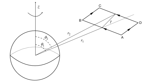
Figure 1: An interference experiment in the Kerr-Newman spacetime, where the setup is put in the asymptotic region. The beams start from the point A and interfere at the point C. The height of the parallelogram is $l$, and the length of the base AB is $s$. The angle between the parallelogram and $r_{1}$ is $\gamma$. Here AB is perpendicular to $\vec{r}_{1}$, $\vec{r}_{2}$, and the axis $z$.

The setup is put in the region satisfying $r_{g}/r\ll 1$, and we take the assumption (29). Besides, we adopt the assumptions in Ref. [10]: (a) The size of the setup is much smaller than its distance from the black hole, such that approximately the coordinates $r$ and $\theta$ keep constant along AB and DC; (b) The energy $\mathcal{E}$ of the particle keeps constant even when it turns direction at B and D (hence the magnitude of the velocity does change at B and D). In the following contents we calculate the gravitational phase difference firstly, then the electromagnetic phase difference.

Same as the formula in Ref. [10], the gravitational phase difference between the paths ADC and ABC is given by

$$\delta\phi^{g}=(\phi_{AD}^{g}+\phi_{DC}^{g})-(\phi_{AB}^{g}+\phi_{BC}^{g})=\delta\phi_{a}+\delta\phi_{b}+\delta\phi_{c},$$ (41)

where

$$\delta\phi_{a} = \frac{1}{\hbar}\bigl{[}(S_{0}^{D})_{DC}t_{AB}+(S_{3}^{D})_{DC}\varphi_{AB}\bigr{]}-\phi_{AB}^{g},$$ (42)

$$\delta\phi_{b} = \frac{1}{\hbar}\bigl{[}(S_{0}^{D})_{DC}-(S_{0}^{A})_{AB}\bigr{]}(t_{DC}-t_{AB}),$$ (43)

$$\delta\phi_{c} = \frac{1}{\hbar}\bigl{[}(S_{3}^{D})_{DC}-(S_{3}^{B})_{BC}\bigr{]}(\varphi_{DC}-\varphi_{AB}).$$ (44)

Here the superscripts A, B, C and D denote the positions, while the subscripts AB, BC, AD and DC denote the paths.

Let us study $\phi^{g}_{AB}$ firstly. According to (36), we get the gravitational phase along the path AB as follows

$$\phi^{g}_{AB}\approx\frac{1}{\hbar}(S_{0}t_{AB}+S_{3}\varphi_{AB}),$$ (45)

because $S_{\beta}$ does not depend on $t$ and $\varphi$ (see (30)), where the assumption (a) has been used, and $t_{AB}=t_{B}-t_{A}$ as well as $\varphi_{AB}=\varphi_{B}-\varphi_{A}$ are defined. Plugging (30) into (45), we obtain

$$\phi^{g}_{AB}\approx\phi^{g}_{0}+\phi^{g}_{Q_{0}}+\phi^{g}_{Q_{q}},$$ (46)

where $\phi^{g}_{0}$ is contributed from $(S_{\beta})_{0}$, while $\phi^{g}_{Q_{0}}$ from $(S_{\beta})_{Q_{0}}$, and $\phi^{g}_{Q_{q}}$ from $(S_{\beta})_{Q_{q}}$:

$$\phi^{g}_{0}=\frac{1}{\hbar}t_{AB}\mathcal{E}\Bigl{(}-\frac{1}{2}\kappa_{g}-\frac{3}{8}\kappa_{g}^{2}-\frac{5}{16}\kappa_{g}^{3}+\frac{1}{2}\cos^{2}\theta_{1}\,\kappa_{a}^{2}\kappa_{g}\Bigr{)}+\frac{1}{\hbar}\varphi_{AB}\sin^{2}\theta_{1}\Bigl{(}\mathcal{E}r_{1}\kappa_{a}\kappa_{g}-\frac{1}{2}\mathcal{L}_{AB}\kappa_{a}^{2}\kappa_{g}+\mathcal{E}r_{1}\kappa_{a}\kappa_{g}^{2}\Bigr{)},$$ (47)

$$\phi^{g}_{Q_{0}}=\frac{1}{4\hbar}t_{AB}\mathcal{E}(2\kappa_{Q}^{2}+3\kappa_{g}\kappa_{Q}^{2})-\frac{1}{\hbar}\varphi_{AB}r_{1}\sin^{2}\theta_{1}\,\mathcal{E}\kappa_{a}\kappa_{Q}^{2},$$ (48)

$$\phi^{g}_{Q_{q}}=\frac{1}{8\hbar}t_{AB}q(4\kappa_{g}\kappa_{Q}+3\kappa_{g}^{2}\kappa_{Q}-4\kappa_{Q}^{3})-\frac{1}{\hbar}\varphi_{AB}qr_{1}\sin^{2}\theta_{1}\,\kappa_{a}\kappa_{g}\kappa_{Q},$$ (49)

where the small quantities $\kappa_{g}$, $\kappa_{a}$ and $\kappa_{Q}$ are defined as follows

$$\kappa_{g}=\frac{r_{g}}{r_{1}},\qquad\kappa_{a}=\frac{a}{r_{1}},\qquad\kappa_{Q}=\frac{Q}{r_{1}}.$$ (50)

Similar to those in Ref. [10], the quantities related to observations are given by (Appendix A)

$$t_{AB}\approx s\Bigl{(}\frac{1}{v\sqrt{g_{00}}}-\frac{g_{03}}{g_{00}\sqrt{\Gamma_{33}}}\Bigr{)},\qquad\varphi_{AB}\approx\frac{s}{\sqrt{\Gamma_{33}}},$$ (51)

$$\mathcal{E}=\frac{m\sqrt{g_{00}}}{\sqrt{1-v^{2}}}+qA_{0},$$ (52)

$$\mathcal{L}=\frac{1}{g_{00}}\bigl{(}-g_{03}+v^{\varphi}\Gamma_{33}\sqrt{g_{00}}\bigr{)}(\mathcal{E}-qA_{0})-qA_{3},$$ (53)

where $s\ll\sqrt{\Gamma_{33}}$ is assumed, with the three-velocity and the three-dimensional metric tenor defined by [13]

$$v^{k}=\frac{\mbox{d}x^{k}}{\sqrt{g_{00}}(\mbox{d}x^{0}+\frac{g_{0i}}{g_{00}}\mbox{d}x^{i})},\qquad\Gamma_{ij}=-g_{ij}+\frac{g_{0i}g_{0j}}{g_{00}}.$$ (54)

Now we return to the phase difference $\delta\phi^{g}$. Same as the procedure in Ref. [10], plugging (30) and (46) into (41), and using (51), (52) and (53), as well as the following relations

$$r_{2}\approx r_{1}+\frac{l\cos\gamma}{\sqrt{-g_{11}(r_{1},\theta_{1})}},\qquad\theta_{2}\approx\Bigl{|}\theta_{1}-\frac{l\sin\gamma}{\sqrt{-g_{22}(r_{1},\theta_{1})}}\Bigr{|},$$ (55)

we expand $\delta\phi^{g}$ in the neighborhoods of $r_{1}$ and $\theta_{1}$ to the first order of $l/r_{1}$. Finally we derive

$$\delta\phi^{g}\approx\delta\phi^{g}_{0}+\delta\phi^{g}_{Q}+\delta\phi^{g}_{q},$$ (56)

where

$$\delta\phi^{g}_{0} = \frac{mls}{\hbar r_{1}\sqrt{1-v^{2}}}\Bigl{\{}\frac{1}{v}\Bigl{[}\cos\gamma\,\Bigl{(}\frac{r_{g}}{2r_{1}}+\frac{r_{g}^{2}}{2r_{1}^{2}}+\frac{r_{g}^{3}}{2r_{1}^{3}}+\frac{a^{2}r_{g}}{4r_{1}^{3}}\bigl{(}1-7\cos^{2}\theta_{1}\bigr{)}\Bigr{)}+\sin(2\theta_{1})\sin\gamma\,\frac{a^{2}r_{g}}{2r_{1}^{3}}\Bigr{]}$$ (57)

$$+\frac{a^{2}r_{g}}{r_{1}^{3}}\sin\theta_{1}\,\Bigl{[}v\Bigl{(}\cos\gamma\,\sin\theta_{1}+\frac{3}{2}\sin\gamma\,\cos\theta_{1}\Bigr{)}+\frac{1}{2}\sin(\theta_{1}-\gamma)\Bigl{(}v-\sqrt{v^{2}-(v^{r})^{2}-(r_{1}v^{\theta})^{2}}\Bigr{)}\Bigr{]}$$

$$-\frac{ar_{g}}{r_{1}^{2}}\Bigl{(}2\cos\theta_{1}\,\sin\gamma+\cos\gamma\,\sin\theta_{1}\Bigr{)}-\frac{ar_{g}^{2}}{r_{1}^{3}}\Bigl{(}\cos\theta_{1}\,\sin\gamma+\frac{3}{2}\cos\gamma\,\sin\theta_{1}\Bigr{)}\Bigr{\}},$$

$$\delta\phi^{g}_{Q} = \frac{mls}{\hbar r_{1}\sqrt{1-v^{2}}}\Bigl{[}-\frac{1}{v}\cos\gamma\,\Bigl{(}\frac{Q^{2}}{r_{1}^{2}}+\frac{3r_{g}Q^{2}}{2r_{1}^{3}}\Bigr{)}+2\sin(\theta_{1}+\gamma)\frac{aQ^{2}}{r_{1}^{3}}\Bigr{]},$$ (58)

$$\delta\phi^{g}_{q} = \frac{qls}{\hbar r_{1}}\Bigl{[}\frac{1}{v}\cos\gamma\,\Bigl{(}-\frac{r_{g}Q}{2r_{1}^{2}}-\frac{3r_{g}^{2}Q}{8r_{1}^{3}}+\frac{Q^{3}}{2r_{1}^{3}}\Bigr{)}+\cos\gamma\,\sin\theta_{1}\,\frac{ar_{g}Q}{r_{1}^{3}}\Bigr{]},$$ (59)

where $v^{r}$ and $v^{\theta}$ defined by (54) are the components of the velocity at B along the path BC. The term (57) is in agreement with the result (75) in Ref. [10]. Indeed, if we let $Q=q=0$, the gravitational phase difference is reduced to $\delta\phi_{0}^{g}$, corresponding to the phase difference in the Kerr spacetime.

As for the electromagnetic phase difference, repeating the above calculations, we find

$$\delta\phi^{e} \approx \frac{qls}{\hbar r_{1}}\Bigl{\{}\frac{1}{v}\Bigl{[}-\frac{Q}{r_{1}}\cos\gamma+\frac{a^{2}Q}{4r_{1}^{3}}\Bigl{(}\cos\gamma\,\bigl{(}5+7\cos(2\theta_{1})\bigr{)}-4\sin\gamma\,\sin(2\theta_{1})\Bigr{)}\Bigr{]}$$ (60)

$$+\frac{aQ}{r_{1}^{2}}\bigl{(}2\sin\gamma\,\cos\theta_{1}+\cos\gamma\,\sin\theta_{1}\bigr{)}+\frac{ar_{g}Q}{2r_{1}^{3}}\cos\gamma\,\sin\theta_{1}\Bigr{\}}.$$

Therefore, the gravitational-electromagnetic phase difference between the paths ABC and ADC is

$$\delta\phi_{\rm ge}=\delta\phi^{g}+\delta\phi^{e}=\delta\phi^{g}_{0}+\delta\phi^{g}_{Q}+\delta\phi^{g}_{q}+\delta\phi^{e},$$ (61)

with $\delta\phi^{g}_{0}$, $\delta\phi^{g}_{Q}$, $\delta\phi^{g}_{q}$, and $\delta\phi^{e}$ given in (57), (58), (59) and (60) respectively. Similar to Ref. [10], we flip the parallelogram along the height $l$ such that A and B swap, to get a new phase difference $\delta\phi_{\rm ge}^{\prime}$ (which is derived by the same way as $\delta\phi_{\rm ge}$ but replacing $\varphi_{AB}$ with $-\varphi_{AB}$). This process causes a fringe shift

$$n=\biggl{|}\frac{\delta\phi_{\rm ge}^{\prime}-\delta\phi_{\rm ge}}{2\pi}\biggr{|}=\bigl{|}n^{g}_{0}+n^{g}_{Q}+n^{g}_{q}+n^{e}\bigr{|},$$ (62)

where

$$n^{g}_{0}=\frac{mls}{\pi\hbar r_{1}\sqrt{1-v^{2}}}\Bigl{[}\frac{ar_{g}^{2}}{r_{1}^{3}}\sin(\gamma+\theta_{1})+\frac{ar_{g}}{r_{1}^{2}}\bigl{(}2\sin\gamma\,\cos\theta_{1}+\cos\gamma\,\sin\theta_{1}\bigr{)}\Bigr{]},$$ (63)

$$n^{g}_{Q}=-\frac{2mls}{\pi\hbar r_{1}\sqrt{1-v^{2}}}\sin(\gamma+\theta_{1})\frac{aQ^{2}}{r_{1}^{3}},$$ (64)

$$n^{g}_{q}=-\frac{qls}{\pi\hbar r_{1}}\cos\gamma\,\sin\theta_{1}\frac{ar_{g}Q}{r_{1}^{3}},$$ (65)

$$n^{e}=\frac{qls}{2\pi\hbar r_{1}}\Bigl{[}-\frac{2aQ}{r_{1}^{2}}\Bigl{(}2\sin\gamma\cos\theta_{1}+\cos\gamma\sin\theta_{1}\Bigr{)}+\cos\gamma\,\sin\theta_{1}\,\frac{ar_{g}Q}{r_{1}^{3}}\Bigr{]}.$$ (66)

Besides, we can rotate the parallelogram along the axis AB from the angle $\gamma=0$ to $\gamma=\pi$, producing a fringe shift

$$N=\biggl{|}\frac{\delta\phi_{\rm ge}(\gamma=0)}{\pi}\biggr{|},$$ (67)

because $\delta\phi_{\rm ge}(\gamma=\pi)=-\delta\phi_{\rm ge}(\gamma=0)$ holds according to (61).

5 Summary and Discussion

The phase of a charged particle in the Kerr-Newman spacetime can be separated into three parts. The first one represents a free particle, the second is the gravitationally induced phase, and the last is the electromagnetic phase. We calculated the gravitational-electromagnetic phase, in the region far away from the Schwardschild radius. The ratios $r_{g}/r$, $a/r$, and $Q/r$ were assumed as small quantities of the same order, then we expanded the phase according to these quantities. As an application, we studied an interference experiment in the Kerr-Newman spacetime, and computed the phase difference as well as the fringe shifts.

Here we show some interesting features appearing in the phase differences. According to (57), (58), (59), and (60), if we let $q=0$, both the electromagnetic phase difference $\delta\phi^{e}$ and the term $\delta\phi^{g}_{q}$ (in the gravitational phase difference $\delta\phi^{g}$) vanish. However, the term $\delta\phi^{g}_{Q}$ for the gravitational phase difference is still there. This term represents the contribution from the charge of the black hole, by means of the gravitation rather than the electromagnetic interaction. Indeed, in the Kerr-Newman spacetime, the charge of the black hole also plays a role in the metric. Another interesting thing is the presence of the term $\delta\phi^{g}_{q}$ in the gravitational phase difference. It means that the charge of the particle contributes to the gravitational phase difference, and $\delta\phi^{g}_{q}$ vanishes if $q=0$ or $Q=0$. This term can be explained by the true that the electromagnetic interaction affects the trajectory of the particle and eventually reflects in the gravitational phase, recalling that the four-momentum in the Kerr-Newman spacetime depends on $qQ$ (see Ref. [16]). But why does not the mass of the particle contribute to the electromagnetic phase difference, considering that the gravitational interaction also affects the path of the particle when we compute the electromagnetic phase? Such difference between $\delta\phi^{g}$ and $\delta\phi^{e}$ may be explained by the universality of the gravitation and the non-universality of the electromagnetic interaction. Given that the integrals for the phases in this paper are always assumed along the classical trajectories of the particle, the paths are independent on the mass of the particle but depend on its charge. Therefore, the charge of the particle appears in the gravitational phase difference, while its mass is absent in the electromagnetic phase difference.

Now we extend our results to the case of a dyonic Kerr-Newman black hole which has an electric charge $Q$ and a magnetic charge $P$. For the metric of such black hole, we only need to replace the expression of $R_{0}$ in (9) by [16]

$$R_{0}=2M-\frac{Q^{2}+P^{2}}{r},$$ (68)

and (21) should be changed to [16, 19, 20, 21]

$$A_{\mu}\mbox{d}x^{\mu}=\frac{Qr}{\rho^{2}}\bigl{(}\mbox{d}t-a\sin^{2}\theta\mbox{d}\varphi\bigr{)}-\frac{P}{\rho^{2}}\cos\theta\,\bigl{[}a\mbox{d}t-(r^{2}+a^{2})\mbox{d}\varphi\bigr{]}.$$ (69)

Correspondingly, for the function $S_{\beta}$, we need to replacing the new metric, new electromagnetic potential, and new four-momentum into (22), where the new expressions for $P^{1}$ and $P^{2}$ are [16]

$$P^{1} = m\frac{dr}{d\tau}=\pm\frac{1}{\rho^{2}}\sqrt{\bigl{[}(r^{2}+a^{2})\mathcal{E}-a\mathcal{L}-qQr\bigr{]}^{2}-m^{2}(r^{2}+K)(r^{2}-2Mr+a^{2}+Q^{2}+P^{2})},$$ (70)

$$P^{2} = m\frac{d\theta}{d\tau}=\pm\frac{1}{\rho^{2}}\sqrt{m^{2}K-m^{2}a^{2}\cos^{2}\theta-\frac{1}{\sin^{2}\theta}(a\mathcal{E}\sin^{2}\theta-\mathcal{L}-qP\cos\theta)^{2}}.$$ (71)

Then repeating the calculations in Sec. 4 for the interference experiment, we find the gravitational phase difference:

$$\delta\phi^{\rm g}\approx\delta\phi^{\rm g}_{0}+\delta\phi^{\rm g}_{QP}+\delta\phi^{\rm g}_{q},$$ (72)

where

$$\delta\phi^{\rm g}_{0} = \frac{mls}{\hbar r_{1}\sqrt{1-v^{2}}}\Bigl{\{}\frac{1}{v}\Bigl{[}\cos\gamma\,\Bigl{(}\frac{r_{g}}{2r_{1}}+\frac{r_{g}^{2}}{2r_{1}^{2}}+\frac{r_{g}^{3}}{2r_{1}^{3}}+\frac{a^{2}r_{g}}{4r_{1}^{3}}\bigl{(}1-7\cos^{2}\theta_{1}\bigr{)}\Bigr{)}+\sin(2\theta_{1})\sin\gamma\,\frac{a^{2}r_{g}}{2r_{1}^{3}}\Bigr{]}$$ (73)

$$+\frac{a^{2}r_{g}}{r_{1}^{3}}\sin\theta_{1}\,\Bigl{[}v\Bigl{(}\cos\gamma\,\sin\theta_{1}+\frac{3}{2}\sin\gamma\,\cos\theta_{1}\Bigr{)}+\frac{1}{2}\sin(\theta_{1}-\gamma)\Bigl{(}v-\sqrt{v^{2}-(v^{r})^{2}-(r_{1}v^{\theta})^{2}}\Bigr{)}\Bigr{]}$$

$$-\frac{ar_{g}}{r_{1}^{2}}\Bigl{(}2\cos\theta_{1}\,\sin\gamma+\cos\gamma\,\sin\theta_{1}\Bigr{)}-\frac{ar_{g}^{2}}{r_{1}^{3}}\Bigl{(}\cos\theta_{1}\,\sin\gamma+\frac{3}{2}\cos\gamma\,\sin\theta_{1}\Bigr{)}\Bigr{\}},$$

$$\delta\phi^{\rm g}_{QP} = \frac{mls}{\hbar r_{1}\sqrt{1-v^{2}}}\Bigl{[}-\frac{1}{v}\cos\gamma\,\Bigl{(}\frac{Q^{2}+P^{2}}{r_{1}^{2}}+\frac{3r_{g}(Q^{2}+P^{2})}{2r_{1}^{3}}\Bigr{)}+2\sin(\theta_{1}+\gamma)\frac{a(Q^{2}+P^{2})}{r_{1}^{3}}\Bigr{]},$$ (74)

$$\delta\phi^{\rm g}_{q} = \frac{qls}{\hbar r_{1}}\Bigl{[}\frac{1}{v}\cos\gamma\,\Bigl{(}-\frac{r_{g}Q}{2r_{1}^{2}}-\frac{3r_{g}^{2}Q}{8r_{1}^{3}}+\frac{Q^{3}}{2r_{1}^{3}}\Bigr{)}+\cos\gamma\,\sin\theta_{1}\,\frac{ar_{g}Q}{r_{1}^{3}}$$ (75)

$$+\frac{\cos\gamma}{2v}\frac{P^{2}Q}{r_{1}^{3}}+\frac{1}{4v}\Bigl{(}\cos(\gamma-\theta_{1})+3\cos(\gamma+\theta_{1})\Bigr{)}\frac{Par_{g}}{r_{1}^{3}}\Bigr{]},$$

and the electromagnetic phase difference:

$$\delta\phi^{\rm e} \approx \frac{qls}{\hbar r_{1}}\Bigl{\{}\frac{1}{v}\Bigl{[}-\frac{Q}{r_{1}}\cos\gamma+\frac{a^{2}Q}{4r_{1}^{3}}\Bigl{(}\cos\gamma\,\bigl{(}5+7\cos(2\theta_{1})\bigr{)}-4\sin\gamma\,\sin(2\theta_{1})\Bigr{)}\Bigr{]}$$ (76)

$$+\frac{aQ}{r_{1}^{2}}\bigl{(}2\sin\gamma\,\cos\theta_{1}+\cos\gamma\,\sin\theta_{1}\bigr{)}+\frac{ar_{g}Q}{2r_{1}^{3}}\cos\gamma\,\sin\theta_{1}$$

$$+\frac{P}{r_{1}}\sin\gamma+\frac{1}{v}\Bigl{[}\frac{Pa}{r_{1}^{2}}\bigl{(}2\cos\gamma\,\cos\theta_{1}-\sin\gamma\,\sin\theta_{1}\bigr{)}-\frac{Par_{g}}{2r_{1}^{3}}\sin\gamma\,\sin\theta_{1}\Bigr{]}$$

$$-\frac{Pa^{2}}{8r_{1}^{3}}\Bigl{(}10\sin\gamma+3\sin(\gamma-2\theta_{1})+11\sin(\gamma+2\theta_{1})\Bigr{)}\Bigr{\}}.$$

Finally, the gravitational-electromagnetic phase difference is given by $\delta\phi^{\rm ge}=\delta\phi^{\rm g}+\delta\phi^{\rm e}$.

Furthermore, we can extend these results to the case of dyonic particles which propagate in the field of a dyonic Kerr-Newman black hole. The action for a particle in such spacetime is

$$S=\int(-m\mbox{d}s-qA_{\mu}\mbox{d}x^{\mu}-g\tilde{A}_{\mu}\mbox{d}x^{\mu}),$$ (79)

where $q$ and $g$ are the electric charge and the magnetic charge of the particle respectively, and $\tilde{A}_{\mu}$ is the potential of the dual filed $\tilde{F}_{\mu\nu}$. By replacing $Q$ with $P$, and $P$ with $-Q$ in (69), the expression for $\tilde{A}_{\mu}$ can be obtained [16]. In the case of dyonic particles, we do not need to repeat the calculations in Sec. 4. Instead, we take a simpler way. Following Ref. [16], we define new charges

$$\hat{Q}=\frac{qQ+gP}{\sqrt{q^{2}+g^{2}}},\qquad\hat{P}=\frac{qP-gQ}{\sqrt{q^{2}+g^{2}}},\qquad\hat{q}=\sqrt{q^{2}+g^{2}},$$ (80)

and a new metric $\hat{g}_{\mu\nu}$ as well as a new electromagnetic potential $\hat{A}_{\mu}$, where $\hat{g}_{\mu\nu}$ and $\hat{A}_{\mu}$ are obtained by replacing $Q$ with $\hat{Q}$, and $P$ with $\hat{P}$ in (68) and (69). One can check

$$\hat{g}_{\mu\nu}=g_{\mu\nu},\qquad\hat{q}\hat{A}_{\mu}=qA_{\mu}+g\tilde{A}_{\mu}.$$ (81)

In this way, the action (79) can be written as

$$S=\int(-m\mbox{d}s-\hat{q}\hat{A}_{\mu}\mbox{d}x^{\mu}).$$ (82)

Evidently the action (82) is not different from the case of a particle without magnetic charge, except that $Q$, $P$, $q$, $g_{\mu\nu}$, and $A_{\mu}$ should be replaced by $\hat{Q}$, $\hat{P}$, $\hat{q}$, $\hat{g}_{\mu\nu}$, and $\hat{A}_{\mu}$ respectively. Given that the gravitational-electromagnetic phase is derived from the action, it is obtained also by using the above substitutions to the old one. Therefore, for the gravitational phase difference and the electromagnetic phase difference in the interference experiment, we only need to replace $Q$ with $\hat{Q}$, $P$ with $\hat{P}$, and $q$ with $\hat{q}$ in the expressions (72) and (76), such that the gravitational-electromagnetic phase difference is

$$\delta\phi^{\rm dyon}_{\rm ge}=\delta\phi^{\rm g}(Q\rightarrow\hat{Q},P\rightarrow\hat{P},q\rightarrow\hat{q})+\delta\phi^{\rm e}(Q\rightarrow\hat{Q},P\rightarrow\hat{P},q\rightarrow\hat{q}).$$ (83)

Appendix A The energy and momentum in the constant gravitational field

In this appendix, we derive the expressions of $t_{AB}$, $\varphi_{AB}$, $\mathcal{E}$, and $\mathcal{L}$ given in Sec. 4. As for the first two quantities, we can take directly the result (73) in Ref. [10]. But here we would like to discuss a general constant gravitational field, then apply the results to the Kerr-Newman spacetime to find these quantities.

For a constant gravitational field, the four-velocity of a massive particle is given by [13]

$$u^{0}=\frac{1}{\sqrt{1-v^{2}}}\Bigl{(}\frac{1}{\sqrt{g_{00}}}-\frac{g_{0k}}{g_{00}}v^{k}\Bigr{)},\qquad u^{j}=\frac{v^{j}}{\sqrt{1-v^{2}}},$$ (84)

where $v^{j}$ is defined in (54), and the velocity $v$ as well as the proper length $L$ are defined by

$$v^{2}=\Gamma_{ij}v^{i}v^{j},\qquad\mbox{d}L^{2}=\Gamma_{ij}\mbox{d}x^{i}\mbox{d}x^{j}.$$ (85)

To find the accumulated time along a path, let us seek for the relation between $\mbox{d}x^{0}$ and $\mbox{d}L$. For this purpose, dividing $\mbox{d}L^{2}$ by $\mbox{d}s^{2}$, we obtain

$$\frac{\mbox{d}L^{2}}{\mbox{d}s^{2}}=\Gamma_{ij}u^{i}u^{j}=\Gamma_{ij}\frac{v^{i}v^{j}}{1-v^{2}}=\frac{v^{2}}{1-v^{2}},$$ (86)

where (84) and (85) have been used. Then according to (84) and (86), we get

$$\frac{\mbox{d}t}{\mbox{d}L}=\frac{u^{0}}{\mbox{d}L/\mbox{d}s}=\frac{1}{v}\Bigl{(}\frac{1}{\sqrt{g_{00}}}-\frac{g_{0k}}{g_{00}}v^{k}\Bigr{)}\quad\Rightarrow\quad\int v\Bigl{(}\frac{1}{\sqrt{g_{00}}}-\frac{g_{0k}}{g_{00}}v^{k}\Bigr{)}^{-1}\mbox{d}t=\int\mbox{d}L.$$ (87)

Now we discuss the covariant four-momentum for a particle in the constant gravitational field. As for $P_{0}$, plugging (84) into $P_{0}=g_{0\nu}P^{\nu}$ results in [13]

$$P_{0}=\frac{m\sqrt{g_{00}}}{\sqrt{1-v^{2}}}.$$ (88)

While for $P_{j}$, inserting (84) into $P_{j}=g_{j\nu}P^{\nu}$, and using the second equation in (54) as well as (88), we derive

$$P_{j}=\frac{m}{\sqrt{g_{00}(1-v^{2})}}(g_{0j}-\Gamma_{jk}v^{k}\sqrt{g_{00}})=\frac{P_{0}}{g_{00}}(g_{0j}-\Gamma_{jk}v^{k}\sqrt{g_{00}}).$$ (89)

Now we apply these results to the Kerr-Newman spacetime to derive (51), (52), and (53) in Sec. 4. Using (87) on the path AB (where $\mbox{d}r=\mbox{d}\theta=0$), we find the expression of $t_{AB}$ in (51). While for $\varphi_{AB}$ in the second equation of (51), as Ref. [10] shows, it is derived by using the second relation in (85). The conserved energy (52) is obtained by combining (19) with (88). As for the conserved momentum, inserting (89) into (20), we get

$$\mathcal{L}=\frac{P_{0}}{g_{00}}\bigl{(}-g_{03}+\Gamma_{33}\,v^{\varphi}\sqrt{g_{00}}\bigr{)}-qA_{3},$$ (90)

where $\Gamma_{31}=\Gamma_{32}=0$ has been used in the second step (these two components vanish in the Kerr-Newman spacetime, recalling (54)). Then plugging $P_{0}=\mathcal{E}-qA_{0}$ (see (19)) into (90), the expression (53) is derived.

Appendix B The electromagnetic field for the dyonic Kerr-Newman black hole

We find that the expressions of the electromagnetic potential for the dyonic Kerr-Newman black hole are different in some papers [16, 19, 20, 21]. In (69) we take the result in Ref. [20], because in the case $a=0$, such potential generates an electromagnetic field as what we expect (namely, it should looks like the field of a dyonic point object). Let us check this argument. In terms of (69), in the case $a=0$, the electromagnetic field and its duality are (here we adopt the convention $F_{\mu\nu}=\partial_{\mu}A_{\nu}-\partial_{\nu}A_{\mu}$ in Ref. [13])

$$F_{\mu\nu}=\begin{pmatrix}0&Qr^{-2}&0&0\\ -Qr^{-2}&0&0&0\\ 0&0&0&-P\sin\theta\\ 0&0&P\sin\theta&0\end{pmatrix},\qquad\tilde{F}_{\mu\nu}=\begin{pmatrix}0&Pr^{-2}&0&0\\ -Pr^{-2}&0&0&0\\ 0&0&0&Q\sin\theta\\ 0&0&-Q\sin\theta&0\end{pmatrix}.$$ (91)

Transforming them into the cartesian coordinates $K^{\prime}(t,x,y,z)$, we get

$$F^{\prime}_{\mu\nu}=\begin{pmatrix}0&Qxr^{-3}&Qyr^{-3}&Qzr^{-3}\\ -Qxr^{-3}&0&-Pzr^{-3}&Pyr^{-3}\\ -Qyr^{-3}&Pzr^{-3}&0&-Pxr^{-3}\\ -Qzr^{-3}&-Pyr^{-3}&Pxr^{-3}&0\end{pmatrix},\qquad\tilde{F}^{\prime}_{\mu\nu}=\begin{pmatrix}0&Pxr^{-3}&Pyr^{-3}&Pzr^{-3}\\ -Pxr^{-3}&0&Qzr^{-3}&-Qyr^{-3}\\ -Pyr^{-3}&-Qzr^{-3}&0&Qxr^{-3}\\ -Pzr^{-3}&Qyr^{-3}&-Qxr^{-3}&0\end{pmatrix}.$$ (92)

They are what we expect. Indeed, the first expression in (92) looks like the electromagnetic field induced by a dyonic point source, if we refer to the definitions in flat spacetime [13]

$$F^{\prime}_{\mu\nu}=\begin{pmatrix}0&E_{x}&E_{y}&E_{z}\\ -E_{x}&0&-B_{z}&B_{y}\\ -E_{y}&B_{z}&0&-B_{x}\\ -E_{z}&-B_{y}&B_{x}&0\end{pmatrix},\qquad\tilde{F}^{\prime}_{\mu\nu}=\begin{pmatrix}0&B_{x}&B_{y}&B_{z}\\ -B_{x}&0&E_{z}&-E_{y}\\ -B_{y}&-E_{z}&0&E_{x}\\ -B_{z}&E_{y}&-E_{x}&0\end{pmatrix},$$ (93)

where the transformations $\vec{E}\rightarrow\vec{B}$ and $\vec{B}\rightarrow-\vec{E}$ have been used to obtain the dual field [23].

References

[1]
L. Stodolsky,
Gen. Rel. Grav. 11, 391-405 (1979)
doi:10.1007/BF00759302
[2]
A. W. Overhauser and R. Colella,
Phys. Rev. Lett. 33, 12377 (1974)
doi:10.1103/PhysRevLett.33.1237
[3]
R. Colella, A. W. Overhauser and S. A. Werner,
Phys. Rev. Lett. 34, 1472-1474 (1975)
doi:10.1103/PhysRevLett.34.1472
[4]
D. M. Greenberger and A. W. Overhauser,
Rev. Mod. Phys. 51, 43-78 (1979)
doi:10.1103/RevModPhys.51.43
[5]
D. V. Ahluwalia and C. Burgard, Gen. Relat. Gravit. 28, 1161–1170 (1996)
doi:10.1007/BF03218936
[6]
Y. Grossman and H. J. Lipkin,
Phys. Rev. D 55, 2760-2767 (1997)
doi:10.1103/PhysRevD.55.2760
[arXiv:hep-ph/9607201 [hep-ph]].
[7]
R. Aldrovandi and J. G. Pereira,
Fundam. Theor. Phys. 173 (2013)
doi:10.1007/978-94-007-5143-9
[8]
R. Aldrovandi, J. G. Pereira and K. H. Vu,
Class. Quant. Grav. 21, 51-62 (2004)
doi:10.1088/0264-9381/21/1/004
[arXiv:gr-qc/0310110 [gr-qc]].
[9]
Y. Aharonov and D. Bohm,
Phys. Rev. 115, 485-491 (1959)
doi:10.1103/PhysRev.115.485
[10]
Z. Mo and L. Modesto,
Phys. Rev. D 108, 104061 (2023)
doi:10.1103/PhysRevD.108.104061
[arXiv:2311.06535 [gr-qc]].
[11]
T. T. Wu and C. N. Yang,
Phys. Rev. D 12, 3845-3857 (1975)
doi:10.1103/PhysRevD.12.3845
[12]
H. I. Arcos and J. G. Pereira,
Int. J. Mod. Phys. D 13, 2193-2240 (2004)
doi:10.1142/S0218271804006462
[arXiv:gr-qc/0501017 [gr-qc]].
[13]
L. D. Landau and E. M. Lifschits,
Pergamon Press, 1975,
ISBN 978-0-08-018176-9
[14]
J. G. Pereira, T. Vargas and C. M. Zhang,
Class. Quant. Grav. 18, 833-842 (2001)
doi:10.1088/0264-9381/18/5/306
[arXiv:gr-qc/0102070 [gr-qc]].
[15]
C. W. Misner, K. S. Thorne, and J. A. Wheeler, Gravitation (W. H. Freeman, San Francisco, 1973).
[16]
E. Hackmann and H. Xu,
Phys. Rev. D 87, no.12, 124030 (2013)
doi:10.1103/PhysRevD.87.124030
[arXiv:1304.2142 [gr-qc]].
[17]
Y. Mino,
Phys. Rev. D 67, 084027 (2003)
doi:10.1103/PhysRevD.67.084027
[arXiv:gr-qc/0302075 [gr-qc]].
[18]
B. Carter,
Phys. Rev. 174, 1559-1571 (1968)
doi:10.1103/PhysRev.174.1559
[19]
I. Semiz,
Class. Quant. Grav. 7, 353-359 (1990)
doi:10.1088/0264-9381/7/3/009