Fisher information susceptibility for multiparameter quantum estimation

Abstract

We extend the notion of the Fisher information measurement noise susceptibility to the multiparameter quantum estimation scenario. After giving its mathematical definition, we derive an upper and a lower bound to the susceptibility. We then apply these techniques to two paradigmatic examples of multiparameter estimation: the joint estimation of phase and phase-diffusion and the estimation of the different parameters describing the incoherent mixture of optical point sources. Our figure provides clear indications on conditions allowing or hampering robustness of multiparameter measurements.

I Introduction

The characterization of any physical system relies on the precise estimation of the physical parameters entering in its model description. This procedure, which has fundamental importance both from a purely theoretical and from a technological perspective, thus corresponds to a multiparameter estimation problem. The aim of quantum metrology is to derive the ultimate bounds on the parameters’ estimation precision in the quantum realm, and to identify possible enhancements by exploiting quantum resources, such as entanglement and squeezing [1, 2, 3, 4, 5, 6, 7, 8, 9]. While most of the paradigmatic results have been obtained in the context of single-parameter estimation, such as phase and frequency, much attention has also been devoted to the case of multiparameter quantum metrology [10, 11], with a particular emphasis on the estimation of unitary parameters [12, 13, 14, 15, 16, 17], unitary and noise parameters [18, 19, 20, 21, 22] and on the estimation of parameters describing the incoherent mixture of optical point sources [23, 24, 25, 26, 27, 28, 29]. A part from its essential importance mentioned above, the case of multiparameter estimation in quantum mechanics raises important theoretical questions being deeply connected with the (potential) non-commutativity of the optimal measurements for single parameters and a the degree of quantumness of the corresponding statistical models has been thoroughly addressed [30, 31, 32]. Moreover, while in the single-parameter case, the role of entanglement, and more in general of collective operations, is crucial only in the probe state preparation, in the multi-parameter scenario the possibility of measuring collectively many copies of quantum states encoding the set of parameters to be estimated is fundamental for achieving the ultimate bounds on the estimation precision [10, 22, 33].

Undesired interaction with the environment and, more in general, the noise affecting a quantum system is detrimental for quantum metrology, as it happens for most of quantum technologies. This has been extensively shown for the single-parameter scenario, both addressing the derivation of the ultimate bounds on the achievable precision in the presence of noise, and in terms of protocols able to attain these bounds [34, 35, 36, 37, 38, 39, 40, 41, 42], and more recently discussing the multiparameter scenario as in [43]. In all these approaches, the effect of noise is discussed either at the level of the state preparation or of the parameter encoding. Only recently, the impact of noise at the level of the measurement stage has been addressed in different contexts [44, 45, 46]. In particular, in  [45], the authors have investigated the effect on the estimation precision in the case of an imperfect realization of a given quantum measurement; in order to properly quantify this, a new figure of merit, dubbed Fisher Information Measurement Noise Susceptibility (FI MeNoS), was introduced. Our goal is to extend this quantity to the multiparameter scenario, by introducing the Fisher Information Matrix-Suited Measurement Noise Susceptibility (FI MaS MeNoS). Besides giving the corresponding mathematical definition and deriving general formulas that will allow its evaluation, we will focus on two paradigmatic examples: the joint estimation of phase and phase-diffusion with a qubit system, and the estimation of the separation of two close incoherent sources along with other instrumental parameters..

The article is structured as follows: in Sec. II we review the single-parameter FI MeNos introduced in [45], while in Sec. III we define the multi-parameter FI MaS MeNos, along with the derivation of upper and lower bounds. In Sec. IV we apply our definition to the two examples mentioned above: i) the estimation of phase and phase-diffusion encoded in single-qubit systems, evaluating FI MaS MeNoS for separable and collective measurement strategies; ii) the estimation of the separation between two sources using the optimal measurement unaffected by Rayleigh’s course. This naturally turns in to a multiparameter problem when we realise that we must also determine the centroid of the emission as well as the ratio of the two intensities.

II Review of the FI MeNoS for the single-parameter case

In this section we revise the definition and the most important properties of the FI MeNoS introduced in [45], starting by recalling the basic ingredients of single-parameter quantum estimation theory.

We consider a quantum statistical model, that is a family of quantum states $\rho_{\theta}$ labelled by a parameter $\theta$ that one wants to estimate. If one performs a measurement described by a POVM $M$ with elements $\{M_{\alpha}\}$, the quantum statistical model is reduced to classical statistical model $p(\alpha|\theta)$ that corresponds to the conditional probability of obtaining the measurement outcome $\alpha$ given the value of the parameter $\theta$, i.e. $p(\alpha|\theta)=\text{Tr}[\rho_{\theta}M_{\alpha}]$. It is proven that the variance of any unbiased estimator of the parameter $\theta$ is bounded by the so-called Cramér-Rao bound

$$\text{Var}(\theta)\geq\frac{1}{KF[M]},$$ (1)

where $K$ is the number of measurements performed and $F[M]$ is the classical Fisher Information (FI) given by

$$F[M]=\sum_{\alpha}\text{Tr}[\rho_{\theta}M_{\alpha}]l_{\alpha}^{2}$$ (2)

where $l_{\alpha}=\text{Tr}[\partial_{\theta}\rho_{\theta}M_{\alpha}]/\text{Tr}[\rho_{\theta}M_{\alpha}]$ and where the trace $\text{Tr}(\cdot)$ is taken in the Hilbert space corresponding to the density operator $\rho_{\theta}$. The Cramer-Rao bound in Eq. (1), which is asymptotically achievable in the limit of large $K$, shows how the FI $F[M]$ quantifies the precision attainable via a certain POVM $M$, and thus induces a hierarchy between measurements: larger values of FI corresponds to measurements yielding better estimation precision. We finally remark that an ultimate quantum bound can be derived by defining the quantum Fisher information (QFI) as

$$Q=\text{Tr}[\rho_{\theta}L_{\theta}^{2}]\,$$ (3)

where $L_{\theta}$ denotes the symmetric-logarithmic derivative operator defined via the equation $2\partial_{\theta}\rho_{\theta}=L_{\theta}\rho_{\theta}+\rho_{\theta}L_{\theta}$. In fact the following quantum Cramér-Rao bound holds

$$\text{Var}(\theta)\geq\frac{1}{KF[M]}\geq\frac{1}{KQ}.$$ (4)

Also this bound is achievable, in the sense that an optimal POVM $M^{(opt)}$ exists such that $F[M^{(opt)}]=Q$.

In [45], Kurzialek and Demkowicz-Dobrzanski addressed the problem of quantifying how much the Fisher information is sensitive to small changes of the measurement that is actually performed in the experiment. This is described by modifying the target measurement $M$, as $(1-\epsilon)M+\epsilon N$, by adding a noise component $N$, that is a different POVM with elements $\{N_{\alpha}\}$. The FI MeNoS is then defined by first taking the limit of an infinitely small change:

$$\chi[M,N] =\lim_{\epsilon\rightarrow 0}\frac{F[M]-F[(1-\epsilon)M+\epsilon N]}{\epsilon F[M]}$$ (5)

$$=1+\frac{G[N]}{F[M]},$$

with $G[N]=\sum_{\alpha}\text{Tr}[A_{\alpha}N_{\alpha}]$, and $A_{\alpha}=l_{\alpha}^{2}\rho_{\theta}-2l_{\alpha}\partial_{\theta}\rho_{\theta}$. The maximum over all noise POVMs is then found, for which a closed analytical form is obtained

$$\sigma[M] =\max_{N}\chi[M,N]$$

$$=1+\frac{1}{2F[M]}\left(l_{n}^{2}+l_{m}^{2}+\|A_{n}-A_{m}\|_{1}\right),$$ (6)

with the subscripts $n$ and $m$ corresponding to the maximal and minimal value of $l_{\alpha}$, respectively. The expression (6) defines the FI MeNoS.

III The multiparameter FI susceptibility

We now consider the case of multiparameter quantum statistical model $\rho_{\bar{\theta}}$, that is a family of quantum states labeled by a vector of $P$ parameters $\bar{\theta}=\{\theta_{1},\theta_{2},...,\theta_{P}\}$. In this case the Cramér-Rao bound is a matrix inequality for the covariance matrix

$${\bf Cov}(\bar{\theta})\geq\frac{1}{K}{\bf F}[M]^{-1}$$ (7)

where the FI has the form of a matrix ${\bf F}[M]$ with elements

$$F[M]_{jk}=\sum_{\alpha}\text{Tr}[\rho_{\bar{\theta}}M_{\alpha}]l_{\alpha,j}l_{\alpha,k},$$ (8)

Here, we have introduced

$$l_{\alpha,j}=\frac{\text{Tr}[\partial_{j}\rho_{\bar{\theta}}M_{\alpha}]}{\text{Tr}[\rho_{\bar{\theta}}M_{\alpha}]}.$$ (9)

with the short-hand notation $\partial_{j}=\partial_{\theta_{j}}$. Also in the multiparameter case one can define a more fundamental quantum bound via the matrix inequality

$${\bf Cov}(\bar{\theta})\geq\frac{1}{K}{\bf F}[M]^{-1}\geq\frac{1}{K}{\bf Q}^{-1}\,,$$ (10)

that can be translated to a scalar bound as

$$\sum_{j}{\rm Var}(\theta_{j})\geq\frac{1}{K}\text{tr}[{\bf F}[M]^{-1}]\geq\frac{1}{K}\text{tr}[{\bf Q}^{-1}]\,.$$ (11)

Notice that in the formulas above $\text{tr}[{\bf O}]$ denotes the trace taken over the matrix space ${\bf O}$, differently from $\text{Tr}[\cdot]$ in the previous formulas, that denote the trace taken over the Hilbert space corresponding to the quantum states $\rho$. The QFI matrix ${\bf Q}$ elements are defined via the single parameter SLD-operators $L_{j}$ as $Q_{jk}=\text{Tr}[\rho_{\bar{\theta}}(L_{j}L_{k}+L_{k}L_{j})/2]$. However in this case both the matrix bound (10) and the scalar bound (11)) are not in general always achievable and tighter bounds can be derived (see Ref. [10] for more details).

In order to properly define the FI MaS MeNoS, we first introduce a matrix susceptibility at fixed noise $N$, extending the definition (5) for the scalar case:

$${\bm{\Xi}}[M,N]={\bf F}[M]^{-1}\lim_{\epsilon\rightarrow 0}\frac{{\bf F}[M]-{\bf F}[(1-\epsilon)M+\epsilon N]}{\epsilon}$$ (12)

The explicit evaluation of the limit results in the expression

$${\bm{\Xi}}[M,N]={\bf I}+{\bf F}^{-1}[M]{\bf G}[N],$$ (13)

with

$${\bf G}(N)=\sum_{\alpha}\text{Tr}[{\bf A}_{\alpha}N_{\alpha}],$$ (14)

$$A_{\alpha;j,k}=l_{\alpha,j}l_{\alpha,k}\rho_{\theta}-l_{\alpha,j}\partial_{k}\rho_{\theta}-l_{\alpha,k}\partial_{j}\rho_{\theta}.$$

In order to capture the sensitivity of the measurement by a scalar quantity also in the multiparameter scenario, we proceed by identifying the limit in (12) as a derivative on the manifold of the POVMs. This leads to consider Jacobi’s formula for the derivative a generic matrix $\bf O$ with respect to a scalar parameter $h$

$$\frac{d}{dh}\det(\bf O)(h)={\text{tr}}[\text{adj}({\bf O}(h))\frac{d{\bf O}}{dh}],$$ (15)

where $\text{adj}({\bf O})$ denotes the adjugate matrix of $\bf O$. For an invertible matrix, $\text{adj}({\bf O})=\det({\bf O}){\bf O}^{-1}$. The scalar susceptibility $\sigma(h)$ with respect to $h$ can then be defined as

$$\sigma(h) =\text{tr}[{\bf O}^{-1}\frac{d{\bf O}}{dh}]$$ (16)

$$=\frac{1}{\det({\bf O})}\frac{d\det({\bf O})}{dh}.$$

Extending these considerations to the POVM manifold, we get

$$X[M,N]=\lim_{\epsilon\rightarrow 0}\frac{\det({\bf F}[M])-\det({\bf F}[(1-\epsilon)M+\epsilon N])}{\epsilon\det({\bf F}[M])}.$$ (17)

which by means of the property

$$\det({\bf X}+\epsilon{\bf Y})=\det({\bf X})(1+\epsilon\,\text{tr}[{\bf X}^{-1}{\bf Y}])+O(\epsilon^{2}).$$ (18)

leads to

$$X[M,N]=P+\text{tr}[{\bf F}[M]^{-1}{\bf G}[N]]\,.$$ (19)

Remarkably this formula is equivalent to the one that is obtained by taking the trace of the matrix susceptibility ${\bm{\Xi}}[M,N]$ in Eq. (13).

The FI MaS MeNoS can then be defined as in Eq. (6) by maximizing over all the possible noise POVM $N$,

$$\Sigma[M]=\max_{N}X[M,N]\,.$$ (20)

This quantity then captures the robustness of the multiparameter measurement as a whole. The maximization is however a hard task; in the following we will show how a close-formula expression for $\Sigma[M]$ can be in principle obtained, leading to lower and upper bounds that can be easily evaluated. We consider the parametrisation in which the Fisher information matrix is diagonal, viz. the set of parameters $\bar{\varphi}=\{\varphi_{1},\varphi_{2},...,\varphi_{P}\}$, with the short-hand notation $\tilde{\partial}_{j}=\partial_{\varphi_{j}}$, and similarly for $\tilde{l}_{\alpha,j}$, $\tilde{A}_{\alpha;j,k}$, as well as for the Fisher information matrix $\tilde{\bf{F}}[M]$.

We introduce the Jacobian matrix $J_{ij}=\tilde{\partial}_{i}\theta_{j}$, which can be used to link the original and reparametrised FI matrices as

$$\tilde{\bf{F}}=\bf{J}\cdot\bf{F}\cdot\bf{J}^{T},$$ (21)

with its element-wise expression

$$\tilde{F}_{ij}=\sum_{kl}F_{kl}\tilde{\partial}_{i}\theta_{k}\tilde{\partial}_{j}\theta_{l}.$$ (22)

Since $\tilde{\nabla}\rho=\bf{J}\cdot\nabla\rho$, due to the definitions (9) and (14), we have that

$$\tilde{A}_{\alpha;ij}=\sum_{kl}A_{\alpha;kl}\tilde{\partial}_{i}\theta_{k}\tilde{\partial}_{j}\theta_{l},$$ (23)

i.e. the matrix $\bf{G}[N]$ transforms as the FI matrix

$$\tilde{\bf{G}}[N]={\bf J}\cdot{\bf G}[N]\cdot\bf{J}^{T},$$ (24)

as one would expect from the trace invariance in (19); indeed, we have that

$$\text{tr}[{\bf F}[M]^{-1}{\bf G}[N]]=\sum_{j}\tilde{G}_{jj}[N]/\tilde{F}_{jj}.$$ (25)

Therefore, for a fixed choice of $N$, $X(M,N)$ is the sum of the single-parameter susceptibilities associated to the parameters $\varphi_{1},\varphi_{2},...,\varphi_{P}$.

We now introduce the functions

$$f_{\alpha}(\vec{x})=c_{\alpha}\|\vec{x}\|^{2}-\vec{x}\cdot\vec{\delta}_{\alpha},$$ (26)

where $c_{\alpha}=\text{Tr}[\rho_{\bar{\theta}}N_{\alpha}]\geq 0$, and $\delta_{\alpha,j}=2\text{Tr}[\tilde{\partial}_{j}\rho_{\bar{\theta}}N_{\alpha}]/\sqrt{\tilde{F}_{jj}}$, making $f_{\alpha}$ a convex function; in addition, given the vector $\vec{L}_{\alpha}=\{\tilde{l}_{\alpha,1}/\sqrt{\tilde{F}_{11}},\tilde{l}_{\alpha,2}/\sqrt{\tilde{F}_{22}},...,\tilde{l}_{\alpha,P}/\sqrt{\tilde{F}_{PP}}\}$ it results

$$X[M,N]=P+\sum_{\alpha}f_{\alpha}(\vec{L}_{\alpha}).$$ (27)

The vectors $\vec{L}_{\alpha}$ define a convex set in $P$ dimensions. This can be used to restrict the class of noise POVMs over which the maximisation of $X[M,N]$ must be carried out. Due to the convexity of $f_{\alpha}(x)$, this will present a maximum in correspondence of one of the extremal points of the set, that, by rearrangement, correspond to the first $E$ elements $\vec{L}_{1},...,\vec{L}_{E}$. Suppose that $f_{E+1}(\vec{x})$ is maximised for $\vec{x}=\vec{L}_{1}$, and consider a generic noise POVM $N=\{N_{1},N_{2},...,N_{E},N_{E+1},...\}$, as well as its variation $N^{\prime}=\{N_{1}+N_{E+1},N_{2},...,N_{E},0,...\}$: by virtue of (27), we get $X[M,N^{\prime}]-X[M,N]=f_{E+1}(\vec{L}_{1})-f_{E+1}(\vec{L}_{E+1})\geq 0$. This transposes a property of the single-parameter FI MeNoS to the multiparameter case. By the applying the same reasoning, ithe search can be restricted to noise POVMS with only $E$ elements, therefore we get

$$\Sigma[M]=P+\max_{N}\sum_{\alpha=1}^{E}\sum_{j}\frac{\text{Tr}[\tilde{A}_{\alpha;jj}N_{\alpha}]}{\tilde{F}_{jj}},$$ (28)

$$=P+\|\vec{L}_{E}\|^{2}+\max_{N}\sum_{\alpha,j}\frac{\text{Tr}[(\tilde{A}_{\alpha;jj}-\tilde{A}_{E;jj})N_{\alpha}]}{\tilde{F}_{jj}},$$

where in the second line we have used the fact that $N_{E}=I-\sum_{\alpha}N_{\alpha}$. The explicit optimisation of the expression (28) is more cumbersome than in the single-parameter case, since the problem can not be reduced to studying a two-outcome noise POVM as for the single-parameter FI MeNoS [45]. Nevertheless, a closer inspection of this formula naturally leads to a lower and an upper bound for $\Sigma[M]$.

The FI MaS MeNoS is limited from below by any $X[M,N]$ at fixed $N$: we can then chose $N$ as a two-outcome POVM, with components on two of the $E$ extremal points, viz. $\alpha^{\prime}$ and $\alpha^{\prime\prime}$. In this way, the expression (28) can be simplified following the same procedure as for the single-parameter case (6):

$$\Sigma[M] \geq\Sigma_{L}[M]$$

$$\Sigma_{L}[M] =P+\frac{1}{2}\left(\|\vec{L}_{\alpha^{\prime}}\|^{2}+\|\vec{L}_{\alpha^{\prime\prime}}\|^{2}\right)$$

$$\,\,\,+\sum_{j}\frac{\|\tilde{A}_{\alpha^{\prime},jj}-\tilde{A}_{\alpha^{\prime\prime},jj}\|_{1}}{2\tilde{F}_{jj}}$$ (29)

The lower bound can be optimised by taking the maximum over the choice of $\alpha^{\prime}$ and $\alpha^{\prime\prime}$.

As for the upper bound, this is set by the sum of the individual FI MeNoS: by means of the expression (6) applied to the individual susceptibilities a bound is established as

$$\Sigma[M] \leq\Sigma^{U}[M]=\sum_{j}\sigma_{j}[M]$$ (30)

$$\sigma_{j}[M] =1+\frac{1}{2\tilde{F}_{jj}[M]}\left(\tilde{l}_{n_{j}}^{2}+\tilde{l}_{m_{j}}^{2}+\|\tilde{A}_{n_{j},jj}-\tilde{A}_{m_{j},jj}\|_{1}\right)$$

where indexes $n_{j}$ and $m_{j}$, associated to the minimum and maximum respectively, may now differ depending on the parameter.

IV Application to multiparameter quantum estimation problems

We will now address the evaluation of the FI MaS MeNoS $\Sigma[M]$ for measurement strategies in two paradigmatic examples of multiparameter quantum estimation. We will first consider the problem of estimating phase and phase-diffusion via qubit probes [18, 19, 20, 21, 22], and we will then approach the estimation of centroid, separation, and relative intensities of two incoherent point sources [25, 26, 29].

IV.1 Simultaneous estimation of phase and dephasing

We now consider the joint estimation of a phase $\phi$ and dephasing $\Delta$ encoded in a qubit quantum statistical model $\rho_{\bar{\theta}}$, which in the $\sigma_{z}$-basis reads

$$\rho_{\bar{\theta}}=\frac{1}{2}\begin{pmatrix}1&e^{-i\phi-\Delta}\\ e^{i\phi-\Delta}&1\end{pmatrix},\,\,\,\bar{\theta}=(\phi,\Delta)\,.$$ (31)

This has served as a common test for multiparameter estimation [18, 19, 20, 21, 22].

Our aim is to quantify the FI MaS MeNoS associated to the two different strategies: i) a separable-measurement strategy, corresponding to a four-outcome single-qubit POVM $M^{\sf(sep)}$ such that

$$M^{\sf(sep)}_{1} =|+_{x}\rangle\langle+_{x}|/2\,\,\,\, M^{\sf(sep)}_{2} =|-_{x}\rangle\langle-_{x}|/2$$

$$M^{\sf(sep)}_{3} =|+_{y}\rangle\langle+_{y}|/2\,\,\,\, M^{\sf(sep)}_{4} =|-_{y}\rangle\langle-_{y}|/2\,$$ (32)

where $|\pm_{x}\rangle$ and $|\pm_{y}\rangle$ are eigenstates respectively of $\sigma_{x}$ and $\sigma_{y}$ operators; ii) an entangled-measurement strategy on two copies $\rho_{\bar{\theta}}\otimes\rho_{\bar{\theta}}$, corresponding to the Bell measurement POVM

$$M^{\sf(ent)}_{1} =|\Psi_{+}\rangle\langle\Psi_{+}|\,\,\,\, M^{\sf(ent)}_{2} =|\Psi_{-}\rangle\langle\Psi_{-}|$$

$$M^{\sf(ent)}_{3} =|\Phi_{+}\rangle\langle\Phi_{+}|\,\,\,\, M^{\sf(ent)}_{4} =|\Phi_{-}\rangle\langle\Phi_{-}|\,$$ (33)

where $|\Psi_{\pm}\rangle$ and $|\Phi_{\pm}\rangle$ denote the four Bell states. It has been in fact discussed how the use of a Bell-measurement on two copies of the state (31) can result in an improved extraction of FI with respect to separable measurements [22]. In particular, following the idea put forward in [33], one can define a parameter quantifying how the estimation via a certain POVM $M$ acting on $m$ copies of the state $\rho_{\bar{\theta}}$ is far from the multiparameter bound given by

$$r[M]=\frac{m\,\text{tr}[{\bf F}[M]^{-1}]}{\text{tr}[{\bf Q}^{-1}]}\geq 1\,.$$ (34)

The lower bound $r[M]=1$ is achieved whenever the the scalar bound (11) is saturated. One can prove that, given the quantum statistical model $\rho_{\bar{\theta}}$ in Eq. (31), the two SLD-operator satisfy the weak-commutativity condition ${\text{T}r}[\rho_{\bar{\theta}}[L_{\phi},L_{\Delta}]]=0$. This implies that the quantum statistical model is asymptotically classical [10], that is a POVM $M$ acting on an asymptotically large number of copies $m\to\infty$ exists such that the bound (11) is achievable, and thus $r[M]=1$. By considering the two strategies introduced above, one has

$$r[M^{\sf(sep)}] =2\,,$$ (35)

$$r[M^{\sf(ent)}] =\frac{1-2\,e^{4\Delta}}{1-2\,e^{2\Delta}}\,,\,\,\,\text{for}\,\,\phi=\pi/4\,$$ (36)

where $r[M^{\sf(ent)}]$ has been already minimized over the phase parameter $\phi$. One can thus show that for a specific value of the phase $\phi$ and for vanishing dephasing $\Delta\approx 0$ the scalar Cramér-Rao bound (11) is already saturated by implementing a two-copies entangled measurement strategy, while for larger values of dephasing $\Delta\gtrsim 0.27$ the Bell measurement performs worse than the separable one.

Our aim is to investigate the behaviour of the FI MaS MeNoS for the two POVMs in this regime, in order to understand any possible relationship between efficiency in the multiparameter estimation and noise susceptibility. In Fig. 1 we plot the corresponding upper and lower bounds of both $\Sigma[M^{\sf(sep)}]$ and $\Sigma[M^{\sf(ent)}]$ for $\phi=\pi/4$ as a function of $\Delta$. First we observe that $\Sigma_{L}$ and $\Sigma^{U}$ give a reliable information on both multiparameter susceptibilities; more in detail we find that in the limit of vanishing noise $\Delta\to 0$ the entangled measurement susceptibility $\Sigma[M^{\sf(ent)}]$ diverges, while the separable measurement tends to a finite value; one can thus argue that, while allowing to saturate the multiparameter quantum Cramér-Rao bound for vanishing dephasing, the Bell measurement is highly susceptible to noise in its implementations. One however also observes how for intermediate, but small values of dephasing ($\Delta\approx 0.04$) the separable POVM susceptibility becomes larger than the entangled POVM one; there is thus a region of parameters, $0.04\lesssim\Delta\lesssim 0.27$ where the Bell measurement still yields a better estimation of phase and dephasing respect to the separable strategy, and even with a lower susceptibility $\Sigma[M^{\sf(ent)}]<\Sigma[M^{\sf(sep)}]$. In general both susceptibilities are decreasing functions of $\Delta$ and one observes a second crossover point for larger values of dephasing.

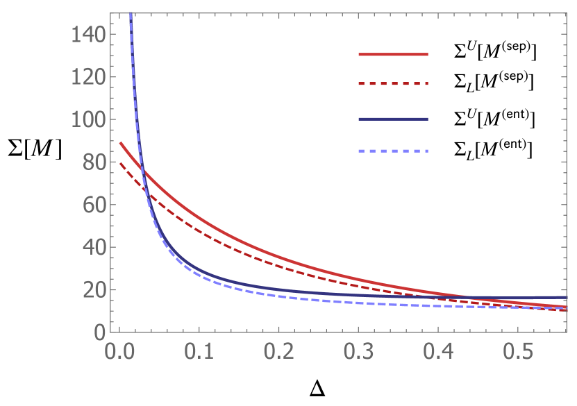
Figure 1: Bounds on the two-parameter susceptibility for respectively a Bell-state measurement and a separable measurement for phase and phase diffusion estimation. The upper and lower bounds are shown as a function of the phase-diffusion parameter $\Delta$ for $\phi=\pi/4$.

IV.2 Multiparameter quantum metrology of incoherent point sources

As our second example, we consider the following quantum statistical model

$$\rho_{\bar{\theta}}=q|\psi_{+}\rangle\langle\psi_{+}|+(1-q)|\psi_{-}\rangle\langle\psi_{-}|$$ (37)

where the states $|\psi_{\pm}\rangle$ are defined by projecting on the $x$-basis as $x$-displaced Gaussian point spread functions

$$\langle x|\psi_{\pm}\rangle=g(x,x_{c}\pm\delta x/2)$$ (38)

with

$$g(x,x_{0})=\frac{1}{(2\pi)^{1/4}}\exp\left\{-\frac{(x-x_{0})^{2}}{4}\right\}$$ (39)

The quantum state in (37) models an incoherent mixture of two point sources. The parameters to be estimated $\bar{\theta}=(x_{c},\delta x,q)$ correspond respectively to the centroid $x_{c}$, the spatial separation $\delta x$ and the relative intensity $q$ of the two sources. A proper analysis on the ultimate quantum limit on this kind of estimation has been extensively discussed [25, 26], showing how the Rayleigh criterion can be in principle overcome also in the multiparameter scenario. While the most immediate interpretation is given in terms of optical sources, the same formalism can be readily applied to a mixture of incoherent short pulses with a given time-delay $\delta x$, and an experimental verification of quantum timing resolution has been shown in [29].

The optimal measurement that has been realized in [29], was previously theoretically investigated in [25, 26]. For small values of $\delta x$ this consists in a $5$-outcome POVM with $M_{j}=|v_{j}\rangle\langle v_{j}|$, $j=0,\dots,3$, and $M_{4}=\mathbbm{1}-\sum_{j=0}^{3}M_{j}$. In particular one shows that

$$|v_{j}\rangle=\sum_{k=0}^{3}w_{j,k}|\Phi_{k}\rangle$$ (40)

where the states $|\Phi_{k}\rangle$ are defined by their projection on the $x$-basis as

$$\langle x|\Phi_{k}\rangle=g(x,x_{m})H_{n}(\frac{x-x_{m}}{\sqrt{2}}),$$ (41)

and $H_{n}(x)$ is the $n$-th Hermite-Gauss polynomial: $H_{n}(x)=(-1)^{n}e^{x^{2}}(d^{n}e^{-x^{2}}/dx^{n})$. The weight matrix entering in (40) is

$${\bf w}=\begin{pmatrix}0&\frac{1}{\sqrt{6}}&\frac{1}{\sqrt{2}}&-\frac{1}{\sqrt{3}}\\ 0&\frac{1}{\sqrt{6}}&-\frac{1}{\sqrt{2}}&-\frac{1}{\sqrt{3}}\\ \sqrt{\frac{2}{5}}&\sqrt{\frac{2}{5}}&0&\frac{1}{\sqrt{5}}\\ -\sqrt{\frac{3}{5}}&\frac{2}{\sqrt{15}}&0&\sqrt{\frac{2}{15}}\end{pmatrix}\,,$$ (42)

while the optimal value of $x_{m}$ is equal to $x_{\rm opt}=x_{c}+(q-1/2)\delta x$ [25]. Contrary to the direct intensity detection, this measurement strategy shows a non-vanishing precision also in the limit $\delta x\rightarrow 0$.

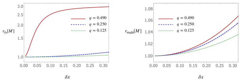
Figure 2: Optimality parameter $r_{\delta x}[M]$ for the estimation of $\delta x$ as a single parameter (left panel), and $r_{\sf multi}[M]$ for the joint estimation of the three parameters $(x_{c},\delta x,q)$ (right panel) as a function of the spatial separation $\delta x$ and for different values of the relative intensity $q$

.

In order to show the optimality of the POVM in the small $\delta x$ regime we consider the parameters

$$r_{\delta x}[M]=\frac{({\bf F}[M]^{-1})_{\delta x,\delta x}}{({\bf Q}^{-1})_{\delta x,\delta x}}\geq 1\,,$$ (43)

and

$$r_{\sf multi}[M]=\frac{\hbox{Tr}[{\bf F}[M]^{-1}]}{\hbox{Tr}[{\bf Q}^{-1}]}\geq 1\,.$$ (44)

The first one $r_{\delta x}[M]$ addresses the estimation of the sources separation $\delta x$, taking into account the centroid $x_{c}$ and the relative intensity $q$ as (unknown) nuisance parameters [47]. The second parameter, as the one define in the previous example in Eq. (34) quantifies the optimality of the measurement strategy for the estimation of all the parameters (in this scenario the measurement is applied to a single copy of the quantum state, i.e. $m=1$). Both quantities (43) and (44) achieve their minimum value when the measurement is optimal, i.e. it saturates the (single- or multi-parameter) quantum Cramér-Rao bound. As we can notice from Fig. 2, the measurement does enjoy indeed such an optimality for both the estimation of $\delta x$ only and for the multiparameter case when the spatial separation $\delta x$ goes to zero. The quality of the estimation of $\delta x$, as captured by (43), decreases as the intensity unbalance $q$ increases; however, even in this regime the multi-parameter estimation seems to perform satisfactorily, $r_{\sf multi}[M]\approx 1$.

We can explain this behaviour by noticing that the three estimated parameters have different scales, thus their uncertainties may vary by orders of magnitude, even when each one reaches its individual Cramér-Rao bound. Consequently, if equal weights are applied, the sum of the variances can be dominated by the contribution of one parameter over the others - specifically, the uncertainty on $q$ is by far the leading term. Since the measurement is optimal for the estimation of $q$, we get $r_{\sf multi}[M]\approx 1$ due to this dominating behaviour regardless the behaviour of the two contributions.

We have then evaluated the upper and lower bounds to the corresponding multiparameter susceptibility $\Sigma[M]$. Remarkably in all the examples we are showing in the following, upper and lower bounds practically coincide, and thus they correspond to the actual susceptibility $\Sigma[M]$. We plot the results as a function of $\delta x$ for different values of $q$ in Fig. 3. We first observe that, unlike the behaviour of $r_{\delta x}[M]$ and $r_{\sf multi}[M]$, $\Sigma[M]$ is not monotonous in $q$. More importantly we also observe that the susceptibility $\Sigma[M]$ is diverging for $\delta x\to 0$: i.e. when the measurement is optimal, small errors in its implementation of the POVM are highly detrimental.

As we pointed out above, we find that in this case $\Sigma[M]=\Sigma^{U}[M]$, i.e. $\Sigma[M]$ is equal to the sum of the single-parameter susceptibilities for the parameters diagonalizing the Fisher information matrix ${\bf F}[M]$, namely $(\varphi_{1},\varphi_{2},\varphi_{3})$. Since $\Sigma[M]$ goes to infinity when $\delta x\to 0$, there must be at least one of these, say $\varphi_{1}$, whose associated susceptibility diverges. The transformation matrix changing the parameters from the parameters $(x_{c},\delta x,q)$ to $(\varphi_{1},\varphi_{2},\varphi_{3})$ is typically full rank, hence each one of these physical parameters will have a component on $\varphi_{1}$. Its diverging susceptibility will then affect the estimation of all parameters, indicating we should not expect particular resilience of any of the three.

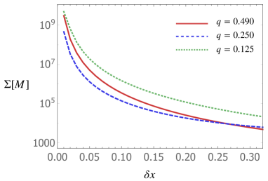
Figure 3: Multiparameter susceptibility $\Sigma[M]$ for the optimal POVM for the estimation of incoherent point sources as a function of the spatial separation $\delta x$ and for different values of the relative intensity $q$.

V Conclusions and outlooks

The analysis of multiparameter measurements is beset on all sides by the noncommutativity of the individual optimal measurements, as well as by statistical correlations. We have nevertheless succeeded in finding a workable definition for the susceptibility to measurement noise; this is able to provide concise information in the form of a scalar figure. The actual maximisation of the figure remains a hard problem, but an upper and a lower bound can be established. Our examples show these bounds can be sufficiently tight to be useful.

Our work enriches the toolkit for the inspection of metrological schemes, being applicable to classical and quantum schemes equally well. Future developments will consider Bayesian schemes, which may affect robustness through prior knowledge, as well as different weighting among the parameters.

References

- Giovannetti et al. [2004] V. Giovannetti, S. Lloyd, and L. Maccone, Quantum-enhanced measurements: Beating the standard quantum limit, Science 306, 1330 (2004), https://science.sciencemag.org/content/306/5700/1330.full.pdf .
- Giovannetti et al. [2006] V. Giovannetti, S. Lloyd, and L. Maccone, Quantum Metrology, Phys. Rev. Lett. 96, 010401 (2006).
- Giovannetti et al. [2011] V. Giovannetti, S. Lloyd, and L. Maccone, Advances in quantum metrology, Nat. Photonics 5, 222 (2011), arXiv:arXiv:1102.2318v1 .
- Caves [1981] C. M. Caves, Quantum-mechanical noise in an interferometer, Phys. Rev. D 23, 1693 (1981).
- Paris [2009] M. G. A. Paris, Quantum estimation for quantum technology, Int. J. Quantum Inf. 07, 125 (2009).
- Demkowicz-Dobrzański et al. [2015] R. Demkowicz-Dobrzański, M. Jarzyna, and J. Kołodyński, Quantum Limits in Optical Interferometry, in Prog. Opt. Vol. 60, edited by E. Wolf (Elsevier, Amsterdam, 2015) Chap. 4, pp. 345–435.
- Degen et al. [2017] C. L. Degen, F. Reinhard, and P. Cappellaro, Quantum sensing, Rev. Mod. Phys. 89, 035002 (2017), arXiv:1611.02427 .
- Pirandola et al. [2018] S. Pirandola, B. R. Bardhan, T. Gehring, C. Weedbrook, and S. Lloyd, Advances in photonic quantum sensing, Nat. Photonics 12, 724 (2018), arXiv:1811.01969 .
- Barbieri [2022] M. Barbieri, Optical quantum metrology, PRX Quantum 3, 010202 (2022).
- Albarelli et al. [2020] F. Albarelli, M. Barbieri, M. Genoni, and I. Gianani, A perspective on multiparameter quantum metrology: From theoretical tools to applications in quantum imaging, Physics Letters A 384, 126311 (2020).
- Szczykulska et al. [2016] M. Szczykulska, T. Baumgratz, and A. Datta, Multi-parameter quantum metrology, Adv. Phys. X 1, 621 (2016), arXiv:1604.02615 .
- Genoni et al. [2013] M. G. Genoni, M. G. A. Paris, G. Adesso, H. Nha, P. L. Knight, and M. S. Kim, Optimal estimation of joint parameters in phase space, Phys. Rev. A 87, 012107 (2013), arXiv:1206.4867 .
- Bradshaw et al. [2018] M. Bradshaw, P. K. Lam, and S. M. Assad, Ultimate precision of joint quadrature parameter estimation with a Gaussian probe, Phys. Rev. A 97, 012106 (2018), arXiv:1710.04817 .
- Humphreys et al. [2013] P. C. Humphreys, M. Barbieri, A. Datta, and I. A. Walmsley, Quantum Enhanced Multiple Phase Estimation, Phys. Rev. Lett. 111, 070403 (2013), arXiv:arXiv:1307.7653v1 .
- Gagatsos et al. [2016] C. N. Gagatsos, D. Branford, and A. Datta, Gaussian systems for quantum-enhanced multiple phase estimation, Phys. Rev. A 94, 042342 (2016), arXiv:1605.04819 .
- Knott et al. [2016] P. A. Knott, T. J. Proctor, A. J. Hayes, J. F. Ralph, P. Kok, and J. A. Dunningham, Local versus global strategies in multiparameter estimation, Phys. Rev. A 94, 062312 (2016), arXiv:1601.05912 .
- Pezzè et al. [2017] L. Pezzè, M. A. Ciampini, N. Spagnolo, P. C. Humphreys, A. Datta, I. A. Walmsley, M. Barbieri, F. Sciarrino, and A. Smerzi, Optimal Measurements for Simultaneous Quantum Estimation of Multiple Phases, Phys. Rev. Lett. 119, 130504 (2017), arXiv:1705.03687 .
- Knysh and Durkin [2013] S. I. Knysh and G. A. Durkin, Estimation of phase and diffusion: Combining quantum statistics and classical noise (2013), arXiv:1307.0470 [quant-ph] .
- Vidrighin et al. [2014] M. D. Vidrighin, G. Donati, M. G. Genoni, X.-M. Jin, W. S. Kolthammer, M. S. Kim, A. Datta, M. Barbieri, and I. A. Walmsley, Joint estimation of phase and phase diffusion for quantum metrology, Nature Communications 5, 3532 (2014).
- Altorio et al. [2015] M. Altorio, M. G. Genoni, M. D. Vidrighin, F. Somma, and M. Barbieri, Weak measurements and the joint estimation of phase and phase diffusion, Phys. Rev. A 92, 032114 (2015).
- Szczykulska et al. [2017] M. Szczykulska, T. Baumgratz, and A. Datta, Reaching for the quantum limits in the simultaneous estimation of phase and phase diffusion, Quantum Science and Technology 2, 044004 (2017).
- Roccia et al. [2017] E. Roccia, I. Gianani, L. Mancino, M. Sbroscia, F. Somma, M. G. Genoni, and M. Barbieri, Entangling measurements for multiparameter estimation with two qubits, Quantum Science and Technology 3, 01LT01 (2017).
- Tsang et al. [2016] M. Tsang, R. Nair, and X.-M. Lu, Quantum theory of superresolution for two incoherent optical point sources, Phys. Rev. X 6, 031033 (2016).
- Chrostowski et al. [2017] A. Chrostowski, R. Demkowicz-Dobrzański, M. Jarzyna, and K. Banaszek, On super-resolution imaging as a multiparameter estimation problem, International Journal of Quantum Information 15, 1740005 (2017), https://doi.org/10.1142/S0219749917400056 .
- Rehacek et al. [2017] J. Rehacek, M. Paúr, B. Stoklasa, Z. Hradil, and L. L. Sánchez-Soto, Optimal measurements for resolution beyond the rayleigh limit, Opt. Lett. 42, 231 (2017).
- Řeháček et al. [2018] J. Řeháček, Z. Hradil, D. Koutný, J. Grover, A. Krzic, and L. L. Sánchez-Soto, Optimal measurements for quantum spatial superresolution, Phys. Rev. A 98, 012103 (2018).
- Napoli et al. [2019] C. Napoli, S. Piano, R. Leach, G. Adesso, and T. Tufarelli, Towards superresolution surface metrology: Quantum estimation of angular and axial separations, Phys. Rev. Lett. 122, 140505 (2019).
- Fiderer et al. [2021] L. J. Fiderer, T. Tufarelli, S. Piano, and G. Adesso, General expressions for the quantum fisher information matrix with applications to discrete quantum imaging, PRX Quantum 2, 020308 (2021).
- Ansari et al. [2021] V. Ansari, B. Brecht, J. Gil-Lopez, J. M. Donohue, J. Řeháček, Z. c. v. Hradil, L. L. Sánchez-Soto, and C. Silberhorn, Achieving the ultimate quantum timing resolution, PRX Quantum 2, 010301 (2021).
- Carollo et al. [2019] A. Carollo, B. Spagnolo, A. A. Dubkov, and D. Valenti, On quantumness in multi-parameter quantum estimation, J. Stat. Mech. Theory Exp. 2019, 094010 (2019).
- Razavian et al. [2020] S. Razavian, M. G. A. Paris, and M. G. Genoni, On the quantumness of multiparameter estimation problems for qubit systems, Entropy 22, 10.3390/e22111197 (2020).
- Candeloro et al. [2021] A. Candeloro, M. G. A. Paris, and M. G. Genoni, On the properties of the asymptotic incompatibility measure in multiparameter quantum estimation, Journal of Physics A: Mathematical and Theoretical 54, 485301 (2021).
- Belliardo and Giovannetti [2021] F. Belliardo and V. Giovannetti, Incompatibility in quantum parameter estimation, New Journal of Physics 23, 063055 (2021).
- Fujiwara and Imai [2008] A. Fujiwara and H. Imai, A fibre bundle over manifolds of quantum channels and its application to quantum statistics, J. Phys. A 41, 255304 (2008).
- Escher et al. [2011] B. M. Escher, R. L. de Matos Filho, and L. Davidovich, General framework for estimating the ultimate precision limit in noisy quantum-enhanced metrology, Nat. Phys. 7, 406 (2011), 1201.1693 .
- Demkowicz-Dobrzański et al. [2012] R. Demkowicz-Dobrzański, J. Kołodyński, and M. Guţă, The elusive Heisenberg limit in quantum-enhanced metrology, Nat. Commun. 3, 1063 (2012), 1201.3940 .
- Chaves et al. [2013] R. Chaves, J. B. Brask, M. Markiewicz, J. Kołodyński, and A. Acín, Noisy Metrology beyond the Standard Quantum Limit, Phys. Rev. Lett. 111, 120401 (2013), 1212.3286 .
- Brask et al. [2015] J. B. Brask, R. Chaves, and J. Kołodyński, Improved Quantum Magnetometry beyond the Standard Quantum Limit, Phys. Rev. X 5, 031010 (2015), 1411.0716 .
- Smirne et al. [2016] A. Smirne, J. Kołodyński, S. F. Huelga, and R. Demkowicz-Dobrzański, Ultimate Precision Limits for Noisy Frequency Estimation, Phys. Rev. Lett. 116, 120801 (2016), 1511.02708v1 .
- Albarelli et al. [2018] F. Albarelli, M. A. C. Rossi, D. Tamascelli, and M. G. Genoni, Restoring Heisenberg scaling in noisy quantum metrology by monitoring the environment, Quantum 2, 110 (2018).
- Zhou et al. [2018] S. Zhou, M. Zhang, J. Preskill, and L. Jiang, Achieving the Heisenberg limit in quantum metrology using quantum error correction, Nat. Commun. 9, 78 (2018), 1706.02445 .
- Rossi et al. [2020] M. A. C. Rossi, F. Albarelli, D. Tamascelli, and M. G. Genoni, Noisy quantum metrology enhanced by continuous nondemolition measurement, Phys. Rev. Lett. 125, 200505 (2020).
- Albarelli and Demkowicz-Dobrzański [2022] F. Albarelli and R. Demkowicz-Dobrzański, Probe incompatibility in multiparameter noisy quantum metrology, Phys. Rev. X 12, 011039 (2022).
- Len et al. [2022] Y. L. Len, T. Gefen, A. Retzker, and J. Kołodyński, Quantum metrology with imperfect measurements, Nature Communications 13, 6971 (2022).
- Kurdziałek and Demkowicz-Dobrzański [2023] S. Kurdziałek and R. Demkowicz-Dobrzański, Measurement noise susceptibility in quantum estimation, Phys. Rev. Lett. 130, 160802 (2023).
- Zhou et al. [2023] S. Zhou, S. Michalakis, and T. Gefen, Optimal protocols for quantum metrology with noisy measurements (2023), arXiv:2210.11393 [quant-ph] .
- Suzuki et al. [2020] J. Suzuki, Y. Yang, and M. Hayashi, Quantum state estimation with nuisance parameters, Journal of Physics A: Mathematical and Theoretical 53, 453001 (2020).