Virtual Quantum Markov Chains

Abstract

Quantum Markov chains generalize classical Markov chains for random variables to the quantum realm and exhibit unique inherent properties, making them an important feature in quantum information theory. In this work, we propose the concept of virtual quantum Markov chains (VQMCs), focusing on scenarios where subsystems retain classical information about global systems from measurement statistics. As a generalization of quantum Markov chains, VQMCs characterize states where arbitrary global shadow information can be recovered from subsystems through local quantum operations and measurements. We present an algebraic characterization for virtual quantum Markov chains and show that the virtual quantum recovery is fully determined by the block matrices of a quantum state on its subsystems. Notably, we find a distinction between two classes of tripartite entanglement by showing that the W state is a VQMC while the GHZ state is not. Furthermore, we establish semidefinite programs to determine the optimal sampling overhead and the robustness of virtual quantum Markov chains. We demonstrate the optimal sampling overhead is additive, indicating no free lunch to further reduce the sampling cost of recovery from parallel calls of the VQMC states. Our findings elucidate distinctions between quantum Markov chains and virtual quantum Markov chains, extending our understanding of quantum recovery to scenarios prioritizing classical information from measurement statistics.

1 Introduction

Background.

Quantum recovery refers to the ability to reverse the effects of a quantum operation on a quantum state, allowing for the retrieval of the original state [1, 2, 3]. When this quantum operation involves discarding a subsystem (mathematically represented as a partial trace) of a tripartite quantum state $\rho_{ABC}$, the concept of recoverability becomes intertwined with Quantum Markov Chains [4].

A tripartite quantum state $\rho_{ABC}$ is called a Quantum Markov Chain in order $A\leftrightarrow B\leftrightarrow C$ if there exists a recovery channel ${\cal R}_{B\to BC}$ that can perfectly reconstruct the original whole state from the $B$-part only, i.e.,

$$\rho_{ABC}={\cal R}_{B\to BC}(\rho_{AB}).$$ (1)

There are two main ways to characterize quantum Markov chains. The entropic characterization of quantum Markov chains states that a tripartite state $\rho_{ABC}$ is a quantum Markov chain if and only if the conditional mutual information $I(A\mathrel{\mathop{\mathchar 58\relax}}C|B)_{\rho}$ is zero [1]. The Petz recovery map, a specific quantum channel, can perfectly reverse the action of the partial trace operation for such quantum Markov chains. Moreover, the algebraic characterization of quantum Markov chains is based on the decomposition of the second subsystem [4], i.e., a tripartite state $\rho_{ABC}$ is a quantum Markov chain if and only if system $B$ can be decomposed into a direct sum tensor product

$${\cal H}_{B}=\underset{j}{\bigoplus}\mathcal{H}_{b^{L}_{j}}\otimes{\cal H}_{b^{R}_{j}},\quad\text{s.t.}\>\rho_{ABC}=\underset{j}{\bigoplus}q_{j}\rho_{Ab^{L}_{j}}\otimes\rho_{b^{R}_{j}C},$$ (2)

with states $\rho_{Ab^{L}_{j}}$ on $\mathcal{H}_{A}\otimes\mathcal{H}_{b^{L}_{j}}$ and $\rho_{b^{R}_{j}C}$ on $\mathcal{H}_{b^{R}_{j}}\otimes\mathcal{H}_{C}$ and a probability distribution $\{q_{j}\}$.

Quantum states that have a small conditional mutual information are shown to be approximate quantum Markov chains as they can be approximately recovered [5]. In particular, Fawzi and Renner [5] shows that for any state $\rho_{ABC}$ there exists a recovery channel ${\cal R}_{B\to BC}$ such that

$$I(A\mathrel{\mathop{\mathchar 58\relax}}C|B)_{\rho}\geq-\log F\big{(}\rho_{ABC},{\cal R}_{B\to BC}(\rho_{AB})\big{)}\,,$$ (3)

where $F(\cdot,\cdot)$ denotes the fidelity between quantum states. Substantial efforts have been made to further understand the approximate quantum Markov chains and the recoverability in quantum information theory (see, e.g., [6, 7, 8, 9, 10, 11, 12, 13, 14]).

The existing results systematically characterize how well one can recover the quantum states via quantum operations. However, in major tasks in quantum information processing, the focus is primarily on the information obtained from the measurement outcomes rather than the quantum state itself. Moreover, a quantum state fundamentally serves as an object that encodes the expectation values of all observables. Given this interpretation, it is intuitively expected that recovering a quantum state from a local system $\rho_{AB}$ to a global system $\rho_{ABC}$ is tantamount to retrieving the essential information for extracting the expectation values of any observables. The task of estimating the expectation values of a given set of observables with respect to a quantum state refers to shadow tomography [15]. The expectation values are also known as shadow information [16] and processing such information is of interests in quantum error mitigation [17, 18, 19, 20], distributed quantum computing [21, 22, 23], entanglement detection [24, 25, 26], quantum broadcasting [27, 28], and fault-tolerant quantum computing [29].

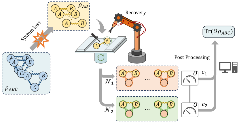
Fig 1: The framework of recovering measurement statistics of a tripartite quantum state with respect to any observable from subsystem $B$ via sampling quantum operations and classical post-processing. The recovery map $\mathscr{R}_{B\rightarrow BC}$ can be simulated via sampling quantum channels ${\cal N}_{1}$ and ${\cal N}_{2}$ regarding the decomposition coefficients $c_{1}$ and $c_{2}$, respectively.

With the aim of understanding the ultimate limit of quantum recoverability, we introduce the virtual quantum Markov chains (VQMCs) to characterize the quantum states whose global shadow information can be recovered from subsystems via quantum operations and post-processing. To be specific, a tripartite quantum state $\rho_{ABC}$ is called a virtual quantum Markov chain in order $A\leftrightarrow B\leftrightarrow C$ if there exists a Hermitian preserving map $\mathscr{R}_{B\rightarrow BC}$ such that

$$\mathscr{R}_{B\rightarrow BC}(\rho_{AB})=\rho_{ABC}.$$ (4)

The above existence of $\mathscr{R}_{B\rightarrow BC}$ ensures that the value of $\operatorname{Tr}(O\rho_{ABC})$ can be retrieved for any observable $O$ from $\rho_{AB}$ via statistically simulating $\mathscr{R}_{B\rightarrow BC}$ using quasiprobability decomposition [18] or measurement-controlled post-processing [20]. The described process of recovering shadow information of a virtual quantum Markov chain is illustrated in Fig. 1.

While much of the existing research focuses on the recovery of quantum states via directly applying quantum operations, our understanding of the recovery of quantum states with respect to unknown observables remains limited. In particular, it is crucial to comprehend the limitations of quantum recovery as the following essential questions arise:

1. What is the structure of a virtual quantum Markov chain?

2. What are the distinctions between quantum Markov chains and virtual quantum Markov chains?

Main contributions.

In this study, we delve into the exploration on the boundary of quantum Markovian dynamics, addressing the two questions mentioned above to better comprehend its limitations. First, we present an algebraic characterization of virtual quantum Markov chains (VQMCs), offering an easily verifiable criterion for determining a quantum state’s qualification as a VQMC. This criterion suggests that a tripartite quantum state can undergo virtual recovery if and only if the kernel of its block matrix on subsystem $B$, conditional on $A$, is included in the kernel of its block matrix on subsystem $BC$, conditional on $A$, (cf. Theorem 1). As a notable application, we show that a quantum state that is classical on the subsystem $C$ is always a VQMC, and particularly, a W state is a VQMC while a GHZ state is not.

Second, we propose the protocol for recovering shadow information for arbitrary observables from a VQMC via sampling local quantum operations and classical post-processing. We explore the sampling overhead of the recovery protocol through semidefinite programming (cf. Sec. 3), shedding light on the distinctions between a quantum Markov chain and a virtual quantum Markov chain. We demonstrate that the optimal sampling overhead for a virtual recovery protocol is additive with respect to the tensor product of states, indicating that a parallel recovering strategy has no advantage over a local protocol, i.e., recovering each state individually. Third, we introduce the approximate virtual quantum Markov chain (cf. Sec. 4), in which we can recover the shadow information with respect to any observable approximately. We also characterize the approximate recoverability via semidefinite programming.

Notations.

We label different quantum systems by capital Latin letters, e.g., $A,B$. The respective Hilbert spaces for these quantum systems are denoted as ${\cal H}_{A}$, ${\cal H}_{B}$, each with dimension $d_{A},d_{B}$. The set of all linear operators on ${\cal H}_{A}$ is denoted by ${\cal L}(A)$, with $I_{A}$ representing the identity operator. We denote by ${\cal L}^{{\dagger}}(A)$ the set of all Hermitian operators on ${\cal H}_{A}$. In particular, we denote ${\cal D}(A)\subseteq{\cal L}^{{\dagger}}(A)$ the set of all density operators being positive semidefinite and trace-one acting on ${\cal H}_{A}$. Throughout the paper, for a tripartite quantum state $\rho_{ABC}\in{\cal D}(A\otimes B\otimes C)$, we denote $\rho_{AB}=\operatorname{Tr}_{C}\rho_{ABC}$. A linear map transforming linear operators in system $A$ to those in system $B$ is termed a quantum channel if it is completely positive and trace-preserving (CPTP), denoted as ${\cal N}_{A\rightarrow B}\mathrel{\mathop{\mathchar 58\relax}}{\cal L}(A)\rightarrow{\cal L}(B)$. The set of all quantum channels from $A$ to $B$ is denoted as $\text{\rm CPTP}(A,B)$. If a map transforms linear operators in ${\cal L}^{{\dagger}}(A)$ to those in ${\cal L}^{{\dagger}}(B)$ and trace-preserving, it is termed a Hermitian-preserving and trace-preserving (HPTP) map. The set of all HPTP maps from $A$ to $B$ is denoted as $\text{\rm HPTP}(A,B)$.

2 Virtual quantum Markov chains

We start with the definition of a virtual quantum Markov chain (VQMC).

Definition 1 (Virtual quantum Markov chain)

A tripartite quantum state $\rho_{ABC}\in{\cal D}(A\otimes B\otimes C)$ is called a virtual quantum Markov chain in order $A\leftrightarrow B\leftrightarrow C$ if there exists a recovery map $\mathscr{R}_{B\rightarrow BC}=\sum_{i}\eta_{i}{\cal N}^{(i)}_{B\rightarrow BC}$ where ${\cal N}^{(i)}_{B\rightarrow BC}\in\text{\rm CPTP}(B,B\otimes C),\eta_{i}\in\mathbb{R}$ such that

$$\mathscr{R}_{B\rightarrow BC}\circ\operatorname{Tr}_{C}(\rho_{ABC})=\rho_{ABC}.$$ (5)

By definition, a quantum Markov chain is also trivially included as a virtual quantum Markov chain. Recall that a quantum Markov chain is a state in which the $C$-part can be reconstructed by locally acting on the $B$-part, thereby recovering the complete information of a state. Extending this, a virtual quantum Markov chain is a state in which the measurement statistics of any observable associated with quantum systems can be reconstructed by exclusively operating on the $B$-part, even when the $C$-part is dismissed. The map $\mathscr{R}_{B\rightarrow BC}$ for a virtual quantum Markov chain is termed as a virtual recovery map. We note that $\mathscr{R}_{B\rightarrow BC}$ can be an unphysical map since it is not necessarily completely positive due to $\eta_{i}$ being arbitrary real numbers. However, $\mathscr{R}_{B\rightarrow BC}$ retains Hermitian-preserving and trace-preserving (HPTP), and can be implemented through quasiprobability decomposition (QPD) [17, 18, 19, 16] and measurement-controlled post-processing [20]. In detail, by sampling quantum channels ${\cal N}_{B\rightarrow BC}^{(i)}$ and performing classical post-processing, we are able to estimate the expectation value of any possible observable in $\rho_{ABC}$. Within this framework, we can accurately retrieve the value of $\operatorname{Tr}(O\rho_{ABC})$ for any observable $O$ under a desired error threshold $\epsilon$ by locally operating on the $B$-part of $\rho_{AB}$.

Following the interpretation of a virtual quantum Markov chain, it is natural to expect that a wider class of states can qualify as VQMCs. But does this extended range include all quantum states? We address this question negatively by presenting a necessary and sufficient condition for a state to be a virtual quantum Markov chain. To characterize the structure inherent in a virtual quantum Markov chain, we first introduce the block matrix of a quantum state on subsystems as follows. For a given $d_{A}\otimes d_{B}$ bipartite quantum state $\rho_{AB}$, we denote $Q_{B}^{(ij)}\mathrel{\mathop{\mathchar 58\relax}}=\langle i|_{A}\rho_{AB}|j\rangle_{A}$ as its block matrix on subsystem $B$ where $\{|i\rangle_{A}\}_{i}$ is the computational basis on subsystem $A$. Consequently, we define the block matrix of $\rho_{AB}$ on subsystem $B$ as

$${{\Theta_{B|A}}}\mathrel{\mathop{\mathchar 58\relax}}=\left[Q_{B}^{(00)},Q_{B}^{(01)},\cdots,Q_{B}^{(d_{A}-1d_{A}-1)}\right].$$ (6)

The kernel, or the null space of ${{\Theta_{B|A}}}$, is given by

$$\ker{{\Theta_{B|A}}}\mathrel{\mathop{\mathchar 58\relax}}=\left\{\mathbf{c}\in\mathbb{C}^{d_{A}^{2}\times 1}\,|\,{{\Theta_{B|A}}}\cdot\mathbf{c}=0\right\},$$ (7)

and the image of ${{\Theta_{B|A}}}$ is given by

$$\operatorname{Im}{{\Theta_{B|A}}}\mathrel{\mathop{\mathchar 58\relax}}=\left\{{{\Theta_{B|A}}}\cdot\mathbf{c}\,|\,\mathbf{c}\in\mathbb{C}^{d_{A}^{2}\times 1}\right\}.$$ (8)

Note that it is straightforward to generalize the block matrix on a subsystem for a multipartite quantum state. A tripartite quantum state $\rho_{ABC}$ can simply be written as $\rho_{ABC}=\sum_{ij}|i\rangle\!\langle j|\otimes Q_{BC}^{(ij)}$ and has

$${{\Theta_{BC|A}}}\mathrel{\mathop{\mathchar 58\relax}}=\left[Q_{BC}^{(00)},Q_{BC}^{(01)},\cdots,Q_{BC}^{(d_{A}-1d_{A}-1)}\right].$$ (9)

Based on the above, the algebraic structure of a VQMC can be characterized as the following theorem.

Proof.

For the "only if" part: By definition, there exists a recovery map $\mathscr{R}_{B\rightarrow BC}$ such that $\mathscr{R}_{B\rightarrow BC}\circ\operatorname{Tr}_{C}(\rho_{ABC})=\rho_{ABC}$, i.e.

$$\forall\,i,j,\ \mathscr{R}_{B\rightarrow BC}\left(Q_{B}^{(ij)}\right)=Q_{BC}^{(ij)}.$$ (11)

For any $\mathbf{c}\in\ker{{\Theta_{B|A}}}$, it is easy to check that

$${{\Theta_{BC|A}}}\cdot\mathbf{c}=\mathscr{R}_{B\rightarrow BC}\left({{\Theta_{B|A}}}\cdot\mathbf{c}\right)=\mathscr{R}_{B\rightarrow BC}\left(0\right)=0.$$ (12)

As a result, $\ker{{\Theta_{B|A}}}\subseteq\ker{{\Theta_{BC|A}}}$ is proved.

For the "if" part: Given a $d_{A}\otimes d_{B}\otimes d_{C}$ tripartite quantum state $\rho_{ABC}$, regarding ${{\Theta_{B|A}}}$ and ${{\Theta_{BC|A}}}$ as linear maps from $\mathbb{C}^{d_{A}^{2}\times 1}$ to $\mathbb{C}^{d_{B}\times d_{B}}$ and $\mathbb{C}^{d_{B}d_{C}\times d_{B}d_{C}}$ respectively, we could check $\operatorname{Tr}_{C}\circ{{\Theta_{BC|A}}}={{\Theta_{B|A}}}$, which implies that $\ker{{\Theta_{BC|A}}}\subseteq\ker{{\Theta_{B|A}}}$. Notice that $\ker{{\Theta_{B|A}}}\subseteq\ker{{\Theta_{BC|A}}}$ as supposed, we find $\ker{{\Theta_{B|A}}}=\ker{{\Theta_{BC|A}}}$ and furthermore the linear space $\operatorname{Im}{{\Theta_{B|A}}}$ is isomorphic to $\operatorname{Im}{{\Theta_{BC|A}}}$. As a result, the surjection $\operatorname{Tr}_{C}$ is just a bijection from $\operatorname{Im}{{\Theta_{BC|A}}}$ to $\operatorname{Im}{{\Theta_{B|A}}}$. Thus a linear map ${\cal M}\mathrel{\mathop{\mathchar 58\relax}}\operatorname{Im}{{\Theta_{B|A}}}\rightarrow\operatorname{Im}{{\Theta_{BC|A}}}$ is denoted as the inverse map of $\operatorname{Tr}_{C}\mathrel{\mathop{\mathchar 58\relax}}\operatorname{Im}{{\Theta_{BC|A}}}\rightarrow\operatorname{Im}{{\Theta_{B|A}}}$.

Denote the orthogonal complement space of the image space $\operatorname{Im}{{\Theta_{B|A}}}\subseteq\mathbb{C}^{d_{B}\times d_{B}}$ as $\left(\operatorname{Im}{{\Theta_{B|A}}}\right)^{\perp}\subseteq\mathbb{C}^{d_{B}\times d_{B}}$, and define linear maps

$$\mathcal{N}\mathrel{\mathop{\mathchar 58\relax}}\left(\operatorname{Im}{{\Theta_{B|A}}}\right)^{\perp}\rightarrow\mathbb{C}^{d_{B}d_{C}\times d_{B}d_{C}},\ M\mapsto\frac{\operatorname{Tr}M}{d_{B}d_{C}}I_{d_{B}d_{C}},$$ (13)

$$\mathscr{R}={\cal M}\oplus\mathcal{N}\mathrel{\mathop{\mathchar 58\relax}}\mathbb{C}^{d_{B}\times d_{B}}\rightarrow\mathbb{C}^{d_{B}d_{C}\times d_{B}d_{C}},\sigma\mapsto{\cal M}\circ\Pi_{\operatorname{Im}{{\Theta_{B|A}}}}(\sigma)+\mathcal{N}\circ\Pi_{\left(\operatorname{Im}{{\Theta_{B|A}}}\right)^{\perp}}(\sigma),$$ (14)

where $\Pi_{\operatorname{Im}{{\Theta_{B|A}}}}$ and $\Pi_{\left(\operatorname{Im}{{\Theta_{B|A}}}\right)^{\perp}}$ denote the projection operators for subspaces $\operatorname{Im}{{\Theta_{B|A}}}$ and $\left(\operatorname{Im}{{\Theta_{B|A}}}\right)^{\perp}$, respectively. To prove $\rho_{ABC}$ is a virtual quantum Markov chain, we only need to check that

$$\mathscr{R}_{B\rightarrow BC}\circ\operatorname{Tr}_{C}(\rho_{ABC})=\rho_{ABC},$$ (15)

and $\mathscr{R}_{B\rightarrow BC}$ is both Hermitian-preserving and trace-preserving. For Eq. (15), we have

$$\mathscr{R}_{B\rightarrow BC}\circ\operatorname{Tr}_{C}(\rho_{ABC})= \sum_{ij}|i\rangle\!\langle j|_{A}\otimes\mathscr{R}_{B\rightarrow BC}\circ\operatorname{Tr}_{C}Q_{BC}^{(ij)}$$ (16)

$$= \sum_{ij}|i\rangle\!\langle j|\otimes\left({\cal M}\circ\Pi_{\operatorname{Im}{{\Theta_{B|A}}}}\circ\operatorname{Tr}_{C}Q_{BC}^{(ij)}+{\cal N}\circ\Pi_{\left(\operatorname{Im}{{\Theta_{B|A}}}\right)^{\perp}}\circ\operatorname{Tr}_{C}Q_{BC}^{(ij)}\right)$$

$$= \sum_{ij}|i\rangle\!\langle j|\otimes\left({\cal M}\circ\operatorname{Tr}_{C}Q_{BC}^{(ij)}+0\right)$$

$$= \sum_{ij}|i\rangle\!\langle j|\otimes Q_{BC}^{(ij)}$$

$$= \rho_{ABC}.$$

For ‘trace-preserving’, we can check that for any $\sigma\in\mathbb{C}^{d_{B}\times d_{B}}$, it follows

$$\operatorname{Tr}\circ\mathscr{R}(\sigma)= \operatorname{Tr}\circ{\cal M}\circ\Pi_{\operatorname{Im}{{\Theta_{B|A}}}}(\sigma)+\operatorname{Tr}\circ{\cal N}\circ\Pi_{\left(\operatorname{Im}{{\Theta_{B|A}}}\right)^{\perp}}(\sigma)$$ (17)

$$= \operatorname{Tr}_{B}\circ\left(\operatorname{Tr}_{C}\circ{\cal M}\circ\Pi_{\operatorname{Im}{{\Theta_{B|A}}}}(\sigma)\right)+\operatorname{Tr}\left(\frac{\operatorname{Tr}\Pi_{(\operatorname{Im}{{\Theta_{B|A}}})^{\perp}}(\sigma)}{d_{B}d_{C}}I_{BC}\right)$$ (18)

$$= \operatorname{Tr}_{B}\circ\left(\Pi_{\operatorname{Im}{{\Theta_{B|A}}}}(\sigma)\right)+\operatorname{Tr}\circ\Pi_{\left(\operatorname{Im}{{\Theta_{B|A}}}\right)^{\perp}}(\sigma)$$ (19)

$$= \operatorname{Tr}\sigma,$$ (20)

where we use the fact that $\forall\,\sigma,\ \Pi_{\operatorname{Im}{{\Theta_{B|A}}}}(\sigma)+\Pi_{\left(\operatorname{Im}{{\Theta_{B|A}}}\right)^{\perp}}(\sigma)=\sigma$.

For ‘Hermitian-preserving’, we note that for any $\sigma\in\mathcal{H}^{B}$, we only need to prove ${\cal M}\circ\Pi_{\operatorname{Im}{{\Theta_{B|A}}}}(\sigma)$ is Hermitian as ${\cal N}\circ\Pi_{\left(\operatorname{Im}{{\Theta_{B|A}}}\right)^{\perp}}(\sigma)$ is always Hermitian. Denote

$$\Pi_{\operatorname{Im}{{\Theta_{B|A}}}}(\sigma)=\sum_{ij}a_{ij}Q_{B}^{(ij)}.$$ (21)

Since $Q_{B}^{(ij)\dagger}=Q_{B}^{(ji)}$, we have $\left(\operatorname{Im}{{\Theta_{B|A}}}\right)^{\dagger}=\operatorname{Im}{{\Theta_{B|A}}}$ and $\left(\operatorname{Im}{{\Theta_{B|A}}}\right)^{\perp\dagger}=\left(\operatorname{Im}{{\Theta_{B|A}}}\right)^{\perp}$. Moreover, by

$$\Pi_{\operatorname{Im}{{\Theta_{B|A}}}}(\sigma)+\Pi_{\left(\operatorname{Im}{{\Theta_{B|A}}}\right)^{\perp}}(\sigma)=\sigma=\sigma^{\dagger}=\Pi_{\operatorname{Im}{{\Theta_{B|A}}}}(\sigma)^{\dagger}+\Pi_{\left(\operatorname{Im}{{\Theta_{B|A}}}\right)^{\perp}}(\sigma)^{\dagger}$$ (22)

$$= \Pi_{\operatorname{Im}{{\Theta_{B|A}}}}\left(\Pi_{\operatorname{Im}{{\Theta_{B|A}}}}(\sigma)^{\dagger}\right)+\Pi_{\left(\operatorname{Im}{{\Theta_{B|A}}}\right)^{\perp}}\left(\Pi_{\left(\operatorname{Im}{{\Theta_{B|A}}}\right)^{\perp}}(\sigma)^{\dagger}\right),$$ (23)

we find both $\Pi_{\operatorname{Im}{{\Theta_{B|A}}}}(\sigma)$ and $\Pi_{\left(\operatorname{Im}{{\Theta_{B|A}}}\right)^{\perp}}(\sigma)\in\mathcal{H}^{B}$. Considering $\sum_{ij}a_{ij}Q_{B}^{(ij)}=\sum_{ij}a_{ij}^{*}Q_{B}^{(ij)\dagger}$ and each $Q_{B}^{(ij)}=Q_{B}^{(ji)\dagger}$, we conclude that each $a_{ij}^{*}=a_{ji}$ based on the arbitrariness of $\sigma$. Finally, by

$$\left({\cal M}\circ\Pi_{\operatorname{Im}{{\Theta_{B|A}}}}(\sigma)\right)^{\dagger}= \left(\sum_{ij}a_{ij}{\cal M}\left(Q_{B}^{(ij)}\right)\right)^{\dagger}=\left(\sum_{ij}a_{ij}Q_{BC}^{(ij)}\right)^{\dagger}=\sum_{ij}a_{ij}^{*}Q_{BC}^{(ij)\dagger}$$ (24)

$$= \sum_{ij}a_{ji}Q_{BC}^{(ji)}=\sum_{ij}a_{ji}{\cal M}\left(Q_{B}^{(ji)}\right)={\cal M}\circ\Pi_{\operatorname{Im}{{\Theta_{B|A}}}}(\sigma),$$ (25)

we completed the proof for Hermitian preserving.     $\sqcap$$\sqcup$

Theorem 1 actually provides an easy-to-check criterion for a state being a VQMC. A straightforward sufficient condition arises: if $\left\{Q_{B}^{(ij)}\right\}_{ij}$ for a state $\rho_{ABC}$ is linear independent, then $\rho_{ABC}$ is a VQMC. Utilizing this theorem, we reveal that the collection of virtual quantum Markov chains does not constitute a convex set.

Proposition 2

The set of all virtual quantum Markov chains is non-convex.

Proof.

Consider the following two tripartite quantum states

$$|s_{1}\rangle=\frac{1}{2}(|001\rangle+|100\rangle+|110\rangle+|111\rangle),|s_{2}\rangle=\frac{1}{2}(|000\rangle+|011\rangle+|101\rangle+|111\rangle).$$ (26)

By direct calculation, we can check that $\left\{Q_{B}^{(ij)}\right\}_{ij}$ for $|s_{1}\rangle\!\langle s_{1}|$ and $|s_{2}\rangle\!\langle s_{2}|$ are independent, thus $|s_{1}\rangle$ and $|s_{2}\rangle$ are VQMCs. However, for the state

$$\rho_{s}=\frac{1}{2}|s_{1}\rangle\!\langle s_{1}|+\frac{1}{2}|s_{2}\rangle\!\langle s_{2}|,$$ (27)

we can check that $Q_{BC}^{(ij)}$ are independent and $Q_{B}^{(01)}=Q_{B}^{(10)}$. Therefore, $\ker{{\Theta_{BC|A}}}=\mathbf{0}$, but there exists $\mathbf{c}\neq\mathbf{0}$ satisfying ${{\Theta_{B|A}}}\cdot\mathbf{c}=0$. By Theorem 1, $\rho_{s}$ is not a virtual quantum Markov chain, which implies that the set of all VQMCs is non-convex.     $\sqcap$$\sqcup$

The non-convex structure of virtual quantum Markov chains aligns with that of quantum Markov chains, suggesting the persistence of non-convex behavior in Markovian dynamics even when we are only concerned with measurement statistics of quantum states. Theorem 1 also implies that if a tripartite state is classical on subsystem $C$, then it is a virtual quantum Markov chain.

Proposition 3

Given a tripartite state $\rho_{ABC}$, if it is classical on $C$, it is a virtual quantum Markov chain.

Proof.

As $\rho_{ABC}$ is classical on $C$, we have $\rho_{ABC}=\sum_{k}p_{k}\rho_{AB}^{(k)}\otimes|k\rangle\!\langle k|_{C}$. It follows

$$Q_{BC}^{(ij)}=\sum_{k}p_{k}\langle i|_{A}\rho_{AB}^{(k)}|j\rangle_{A}\otimes|k\rangle\!\langle k|_{C},\quad Q_{B}^{(ij)}=\sum_{k}p_{k}\langle i|_{A}\rho_{AB}^{(k)}|j\rangle_{A}.$$ (28)

For any $\mathbf{c}\in\ker{{\Theta_{BC|A}}}$, it follows that

$$\sum_{i,j}c_{ij}\left(\sum_{k}p_{k}\langle i|_{A}\rho_{AB}^{(k)}|j\rangle_{A}\otimes|k\rangle\!\langle k|_{C}\right)=\sum_{k}\left(\sum_{i,j}c_{ij}p_{k}\langle i|_{A}\rho_{AB}^{(k)}|j\rangle_{A}\right)\otimes|k\rangle\!\langle k|_{C}=0$$ (29)

which yields

$$\forall k,\quad\sum_{i,j}c_{ij}p_{k}\langle i|_{A}\rho_{AB}^{(k)}|j\rangle_{A}=0.$$ (30)

Thus, we have $\sum_{i,j}c_{ij}Q_{B}^{(ij)}=0$, implying $\mathbf{c}\in\ker{{\Theta_{B|A}}}$. By Theorem 1, we conclude $\rho_{ABC}$ is a virtual quantum Markov chain.     $\sqcap$$\sqcup$

Proposition 3 suggests that if the $C$-part we lose is classical, we can recover the complete classical information $\operatorname{Tr}(O\rho_{ABC})$ for any observable $O$ encoded in $\rho_{ABC}$ through the sampling of local operations and subsequent classical post-processing.

To deepen our understanding of virtual quantum Markov chains, we explore the structure of essential tripartite states. The W state and the GHZ state are two representative non-biseparable states that cannot be transformed (not even probabilistically) into each other by local quantum operations [30]. They play important roles in various quantum information tasks, including quantum communication [31, 32], quantum key distribution [33], and quantum algorithms [34]. Remarkably, neither the W state nor the GHZ state are quantum Markov chains. However, in the realm of virtual quantum Markov chains, a divergence appears: the W state aligns with the characteristics of a virtual quantum Markov chain, whereas the GHZ state does not. This distinction elucidates the complex nature of these states within this broader context of quantum Markovian dynamics.

W state.

A generalized W state is a three-qubit entangled quantum state defined by

$$|W_{\alpha_{0},\alpha_{1}}\rangle=\sqrt{\alpha_{0}}|001\rangle+\sqrt{\alpha_{1}}|010\rangle+\sqrt{1-\alpha_{0}-\alpha_{1}}|100\rangle.$$ (31)

For $\rho_{ABC}=|W_{\alpha_{0},\alpha_{1}}\rangle\!\langle W_{\alpha_{0},\alpha_{1}}|$, we can calculate

$$Q_{B}^{(00)}=\left(\begin{array}[]{cc}\alpha_{0}&0\\ 0&\alpha_{1}\\ \end{array}\right),Q_{B}^{(01)}=\sqrt{1-\alpha_{0}-\alpha_{1}}\left(\begin{array}[]{cc}0&0\\ \sqrt{\alpha_{1}}&0\\ \end{array}\right),$$ (36)

$$Q_{B}^{(10)}=\sqrt{1-\alpha_{0}-\alpha_{1}}\left(\begin{array}[]{cc}0&\sqrt{\alpha_{1}}\\ 0&0\\ \end{array}\right),Q_{B}^{(11)}=\left(\begin{array}[]{cc}1-\alpha_{0}-\alpha_{1}&0\\ 0&0\\ \end{array}\right).$$ (41)

Notice that matrices in $\{Q_{B}^{(ij)}\}_{ij}$ are linear independent and form a basis for $\mathbb{C}^{2\times 2}$. It follows that $\ker{{\Theta_{B|A}}}=\ker{{\Theta_{BC|A}}}=\mathbf{0}$. Therefore, a three-qubit generalized W state is a virtual quantum Markov chain. Particularly, the virtual recovery map $\mathscr{R}_{B\rightarrow BC}$ has a Choi representation as

$$J_{\mathscr{R}}= \frac{|0\rangle\!\langle 0|\otimes Q^{(11)}_{BC}}{1-\alpha_{0}-\alpha_{1}}+\frac{|0\rangle\!\langle 1|\otimes Q^{(10)}_{BC}}{\sqrt{\alpha_{1}(1-\alpha_{0}-\alpha_{1})}}$$ (42)

$$+\frac{|1\rangle\!\langle 0|\otimes Q^{(01)}_{BC}}{\sqrt{\alpha_{0}(1-\alpha_{0}-\alpha_{1})}}+|1\rangle\!\langle 1|\otimes\frac{(1-\alpha_{0}-\alpha_{1})Q^{(00)}_{BC}-\alpha_{0}Q^{(11)}_{BC}}{\alpha_{1}(1-\alpha_{0}-\alpha_{1})}.$$

where $Q^{(ij)}_{BC}$ is the block matrix of $|W_{\alpha_{0},\alpha_{1}}\rangle\!\langle W_{\alpha_{0},\alpha_{1}}|$ on subsystem $BC$.

GHZ state.

A three-qubit GHZ state is a tripartite entangled quantum state defined by

$$|GHZ\rangle=\frac{1}{\sqrt{2}}(|000\rangle+|111\rangle).$$ (43)

For $\rho_{ABC}=|GHZ\rangle\!\langle GHZ|$, we have

$$Q_{BC}^{(00)}=|00\rangle\!\langle 00|/2,Q_{BC}^{(01)}=|00\rangle\!\langle 11|/2,Q_{BC}^{(10)}=|11\rangle\!\langle 00|/2,Q_{BC}^{(11)}=|11\rangle\!\langle 11|/2,$$ (44)

$$Q_{B}^{(00)}=|0\rangle\!\langle 0|/2,Q_{B}^{(01)}=0,Q_{B}^{(10)}=0,Q_{B}^{(11)}=|1\rangle\!\langle 1|/2.$$ (45)

It is easy to check that there is a $\mathbf{c}\in\mathbb{C}^{1\times 4}$ such that ${{\Theta_{B|A}}}\cdot\mathbf{c}=0$ but ${{\Theta_{BC|A}}}\cdot\mathbf{c}\neq 0$. By Theorem 1, the GHZ state is not a virtual quantum Markov chain. It indicates that even when we are only interested in measurement statistics of a GHZ state, we still cannot locally recover the information after discarding the subsystem $C$.

In the above, we demonstrate that a three-qubit W state is a virtual quantum Markov chain, but a three-qubit GHZ state is not. This distinction underscores the essential properties of virtual quantum Markov chains. This suggests that the nature and distribution of quantum entanglement within a system could have profound implications for its Markovian properties when we are only concerned with extracting expectation value, e.g. $\operatorname{Tr}(O\rho)$. Note that after taking a partial trace on system $C$ for the W states, the reduced density operator contains a residual EPR entanglement. The robustness of W-type entanglement contrasts strongly with the GHZ state, which is fully separable after the loss of one qubit. These findings highlight the need for a deeper understanding of the interplay between multipartite quantum entanglement and Markovian dynamics.

Furthermore, we investigate the robustness of these virtual quantum Markov chains regarding specific quantum noise. For example, consider a three-qubit W state and a three-qubit GHZ state affected by three-qubit depolarizing channels ${\cal D}_{p}(\cdot)=(1-p)(\cdot)+pI_{8}/8$ with a noise rate $p\in[0,1]$. We denote the respective states as

$$W(p)=(1-p)|W\rangle\!\langle W|+p\frac{I_{8}}{8},\quad G(p)=(1-p)|GHZ\rangle\!\langle GHZ|+p\frac{I_{8}}{8},$$ (46)

where $|W\rangle$ is defined in Eq. (31) with $\alpha_{0}=\alpha_{1}=1/3$ and $|GHZ\rangle$ is defined in Eq. (43). Then, we have the following results.

Example 1 Let $|W\rangle$ be a three-qubit W state. $W(p)=(1-p)|W\rangle\!\langle W|+pI_{8}/8$ is a virtual quantum Markov chain for $p\in[0,1]$.

Proof.

For $W(p)=(1-p)|W\rangle\!\langle W|+pI_{8}/8$ with $|W\rangle=(|001\rangle+|010\rangle+|100\rangle)/\sqrt{3}$, we can calculate its block matrices on subsystem $BC$ and $B$ as

$$Q_{BC}^{(00)}=\left(\begin{array}[]{cccc}p/8&0&0&0\\ 0&(1-p)/3+p/8&(1-p)/3&0\\ 0&(1-p)/3&(1-p)/3+p/8&0\\ 0&0&0&p/8\\ \end{array}\right),Q_{BC}^{(01)}=\left(\begin{array}[]{cccc}0&0&0&0\\ 1/3&0&0&0\\ 1/3&0&0&0\\ 0&0&0&0\\ \end{array}\right),$$ (55)

$$Q_{BC}^{(10)}=\left(\begin{array}[]{cccc}0&1/3&1/3&0\\ 0&0&0&0\\ 0&0&0&0\\ 0&0&0&0\\ \end{array}\right),Q_{BC}^{(11)}=\left(\begin{array}[]{cccc}(1-p)/3+p/8&0&0&0\\ 0&p/8&0&0\\ 0&0&p/8&0\\ 0&0&0&p/8\\ \end{array}\right),$$ (64)

$$Q_{B}^{(00)}=\left(\begin{array}[]{cc}(1-p)/3+p/4&0\\ 0&(1-p)/3+p/4\\ \end{array}\right),Q_{B}^{(01)}=\left(\begin{array}[]{cc}0&0\\ 1/3&0\\ \end{array}\right),$$ (69)

$$Q_{B}^{(10)}=\left(\begin{array}[]{cc}0&1/3\\ 0&0\\ \end{array}\right),Q_{B}^{(11)}=\left(\begin{array}[]{cc}(1-p)/3+p/4&0\\ 0&p/4\\ \end{array}\right).$$ (74)

We can check that $\{Q_{B}^{(ij)}\}$ is linear independent. By Theorem 1, $W(p)$ is a virtual Markov chain.     $\sqcap$$\sqcup$

Example 2 Let $|GHZ\rangle$ be a three-qubit GHZ state. $G(p)=(1-p)|GHZ\rangle\!\langle GHZ|+pI_{8}/8$ is not a virtual quantum Markov chain for $p\in[0,1)$.

Proof.

For $G(p)=(1-p)|GHZ\rangle\!\langle GHZ|+pI_{8}/8$ with $|GHZ\rangle=(|000\rangle+|111\rangle)/\sqrt{2}$, we can calculate its block matrices on subsystem $BC$ and $B$ as

$$Q_{BC}^{(00)}=\frac{(1-p)}{2}|00\rangle\!\langle 00|+\frac{p}{8}I_{4},Q_{BC}^{(01)}=\frac{(1-p)}{2}|00\rangle\!\langle 11|,Q_{BC}^{(10)}=\frac{(1-p)}{2}|11\rangle\!\langle 00|,$$ (75)

$$Q_{BC}^{(11)}=\frac{(1-p)}{2}|11\rangle\!\langle 11|+\frac{p}{8}I_{4},$$

$$Q_{B}^{(00)}=\frac{(1-p)}{2}|0\rangle\!\langle 0|+\frac{p}{4}I_{2},Q_{B}^{(01)}=0,Q_{B}^{(10)}=0,Q_{B}^{(11)}=\frac{(1-p)}{2}|1\rangle\!\langle 1|+\frac{p}{4}I_{2}.$$

Since $Q_{B}^{(01)}=Q_{B}^{(10)}=0$, it is easy to find a $\mathbf{c}\in\mathbb{C}^{1\times 4}$ such that ${{\Theta_{B|A}}}\cdot\mathbf{c}=0$ but ${{\Theta_{BC|A}}}\cdot\mathbf{c}\neq 0$. By Theorem 1, $G(p)$ is not a virtual quantum Markov chain unless $p=1$.     $\sqcap$$\sqcup$

The above examples reveal intrinsic properties inherent in virtual quantum Markov chains. Notice that the maximally mixed state $I_{8}/8$ is a quantum Markov chain. Example 2 and Example 2 show that the W state and GHZ state maintain their properties of virtual recoverability against depolarizing noise. Example 2 demonstrates that there are cases where a convex combination of VQMCs is still a VQMC even though it is not generally valid. We note that although a GHZ state cannot turn into a VQMC when it is mixed with a maximally mixed state, as shown in Example 2, it becomes a VQMC when mixing with a W state as the following example.

Example 3 Let $|GHZ\rangle$ and $|W\rangle$ be three-qubit GHZ state and W state. For $p\in[0,1],\ GW(p)=p|GHZ\rangle\!\langle GHZ|+(1-p)|W\rangle\!\langle W|$ is not a virtual quantum Markov chain if and only if $p=1$ or $7-3\sqrt{5}$.

Proof.

For $GW(p)=p|GHZ\rangle\!\langle GHZ|+(1-p)|W\rangle\!\langle W|$ with $|GHZ\rangle=(|000\rangle+|111\rangle)/\sqrt{2}$ and $|W\rangle=(|001\rangle+|010\rangle+|100\rangle)/\sqrt{3}$, we can calculate its block matrices on subsystem $BC$ and $B$ as

$$Q_{BC}^{(00)}=\left(\begin{array}[]{cccc}\frac{p}{2}&0&0&0\\ 0&\frac{1-p}{3}&\frac{1-p}{3}&0\\ 0&\frac{1-p}{3}&\frac{1-p}{3}&0\\ 0&0&0&0\\ \end{array}\right),Q_{BC}^{(01)}=\left(\begin{array}[]{cccc}0&0&0&\frac{p}{2}\\ \frac{1-p}{3}&0&0&0\\ \frac{1-p}{3}&0&0&0\\ 0&0&0&0\\ \end{array}\right),$$ (84)

$$Q_{BC}^{(10)}=\left(\begin{array}[]{cccc}0&\frac{1-p}{3}&\frac{1-p}{3}&0\\ 0&0&0&0\\ 0&0&0&0\\ \frac{p}{2}&0&0&0\\ \end{array}\right),Q_{BC}^{(11)}=\left(\begin{array}[]{cccc}\frac{1-p}{3}&0&0&0\\ 0&0&0&0\\ 0&0&0&0\\ 0&0&0&\frac{p}{2}\\ \end{array}\right),$$ (93)

$$Q_{B}^{(00)}=\left(\begin{array}[]{cc}\frac{2+p}{6}&0\\ 0&\frac{1-p}{3}\\ \end{array}\right),Q_{B}^{(01)}=\left(\begin{array}[]{cc}0&0\\ \frac{1-p}{3}&0\\ \end{array}\right),$$ (98)

$$Q_{B}^{(10)}=\left(\begin{array}[]{cc}0&\frac{1-p}{3}\\ 0&0\\ \end{array}\right),Q_{B}^{(11)}=\left(\begin{array}[]{cc}\frac{1-p}{3}&0\\ 0&\frac{p}{2}\\ \end{array}\right).$$ (103)

Since $\ker{{\Theta_{B|A}}}\neq 0$ if only if $\frac{1-p}{3}=0$ or $\frac{2+p}{6}\frac{p}{2}=\frac{1-p}{3}\frac{1-p}{3}$, i.e. $p=1$ or $7-3\sqrt{5}$. It is easy to check that $\ker{{\Theta_{BC|A}}}=0$ for $p=1$ or $p=7-3\sqrt{5}$. Thus, we complete the proof.     $\sqcap$$\sqcup$

VQMC and quantum conditional mutual information.

Besides operational characterization, it is noteworthy that classical Markov chains and quantum Markov chains are interconnected with entropy measures, specifically conditional mutual information and quantum conditional mutual information, respectively. However, we remark that a virtual quantum Markov chain no longer maintains an intrinsic connection with the quantum conditional mutual information. Herein, we present two tripartite states with the same quantum conditional mutual information, but one is a VQMC, and the other is not.

Example 4 Consider two pure three-qubit quantum states given by

$$|\psi_{1}\rangle=\frac{1}{\sqrt{3}}(|010\rangle+|101\rangle+|110\rangle),\;|\psi_{2}\rangle=\frac{1}{\sqrt{3}}(|010\rangle+|011\rangle+|100\rangle).$$ (104)

It is easy to check that $I(A\mathrel{\mathop{\mathchar 58\relax}}C|B)_{\psi_{1}}=I(A\mathrel{\mathop{\mathchar 58\relax}}C|B)_{\psi_{2}}=0.55$. Nonetheless, $|\psi_{1}\rangle$ is not a virtual quantum Markov chain, and $|\psi_{2}\rangle$ is a virtual quantum Markov chain.

Proof.

For $|\psi_{1}\rangle\!\langle\psi_{1}|$, we have

$$Q^{(00)}_{BC}=\frac{1}{3}|10\rangle\!\langle 10|,Q^{(01)}_{BC}=\frac{1}{3}|10\rangle(\langle 01|+\langle 10|),$$ (105)

$$Q^{(10)}_{BC}=\frac{1}{3}(|10\rangle+|01\rangle)\langle 10|,Q^{(11)}_{BC}=\frac{1}{3}(|10\rangle+|01\rangle)(\langle 01|+\langle 10|),$$

and

$$Q^{(00)}_{B}=Q^{(01)}_{B}=Q^{(10)}_{B}=\frac{1}{3}|1\rangle\!\langle 1|,Q^{(11)}_{B}=\frac{1}{3}(|0\rangle\!\langle 0|+|1\rangle\!\langle 1|).$$ (106)

It is direct to check for state $\psi_{1}$, there is a $\mathbf{c}\in\mathbb{C}^{1\times 4}$ such that ${{\Theta_{B|A}}}\cdot\mathbf{c}=0$ while ${{\Theta_{BC|A}}}\cdot\mathbf{c}\neq 0$. Hence, state $|\psi_{1}\rangle$ is not a virtual quantum Markov chain. On the other hand, for state $|\psi_{2}\rangle\!\langle\psi_{2}|$, we have

$$Q^{(00)}_{BC}=\frac{1}{3}(|10\rangle+|11\rangle)(\langle 10|+\langle 11|),Q^{(01)}_{BC}=\frac{1}{3}(|10\rangle+|11\rangle)\langle 00|,$$ (107)

$$Q^{(10)}_{BC}=\frac{1}{3}|00\rangle(\langle 10|+\langle 11|),Q^{(11)}_{BC}=\frac{1}{3}|00\rangle\!\langle 00|,$$

and

$$Q^{(00)}_{B}=\frac{2}{3}|1\rangle\!\langle 1|,Q^{(01)}_{B}=\frac{1}{3}|1\rangle\!\langle 0|,Q^{(10)}_{B}=\frac{1}{3}|0\rangle\!\langle 1|,Q^{(11)}_{B}=\frac{1}{3}|0\rangle\!\langle 0|.$$ (108)

We find sub-matrices $\{Q^{(ij)}_{B}\}_{ij}$ are linear independent and form a basis of $\mathbb{C}^{2\times 2}$. Therefore, $\ker{{\Theta_{B|A}}}=\ker{{\Theta_{BC|A}}}=\mathbf{0}$ and $|\psi_{2}\rangle$ is a virtual Markov chain.     $\sqcap$$\sqcup$

We have seen these two states, despite possessing identical quantum conditional mutual information, exhibit differing characteristics - one constitutes a virtual quantum Markov chain, while the other does not. This discrepancy underscores the divergence between quantum conditional mutual information and the properties of virtual quantum Markov chains, indicating the unique structure of a VQMC different from a quantum Markov chain.

3 Sampling overhead of virtual recovery

For the successful recovery of the measurement statistics of a virtual quantum Markov chain, a quasi-probability decomposition strategy necessitates the consumption of multiple copies of the states [18]. The sampling times required to achieve the desired precision, therefore, characterize the difference between a state being a QMC or a VQMC. In this context, we introduce the sampling overhead of virtual recovery as follows.

Definition 2 (Optimal sampling overhead)

Given a virtual quantum Markov chain $\rho_{ABC}$, the optimal sampling overhead of virtual recovery is defined as

$$\nu(\rho_{ABC})\mathrel{\mathop{\mathchar 58\relax}}=\log\min\Big{\{}c_{1}+c_{2}\big{|}(c_{1}{\cal N}_{1}-c_{2}{\cal N}_{2})(\rho_{AB})=\rho_{ABC},\,c_{1,2}\geq 0,{\cal N}_{1,2}\in\text{\rm CPTP}(B,B\otimes C)\Big{\}}.$$

The sampling overhead of virtual recovery is closely related to the physical implementability of HPTP maps [18] and can be determined via the following semidefinite programmings (SDPs) [35], both of which evaluate to $2^{\nu(\rho_{ABC})}$.

$$\begin{aligned} &\underline{\textbf{Primal Program}}\\ \min&\;\;c_{1}+c_{2}\\ {\rm s.t.}&\;J_{1}\geq 0,J_{2}\geq 0,\\ &\;J_{BB^{\prime}C}=J_{1}-J_{2},\\ &\;\operatorname{Tr}_{B^{\prime}C}J_{1}=c_{1}I_{B},\operatorname{Tr}_{B^{\prime}C}J_{2}=c_{2}I_{B},\\ &\;\operatorname{Tr}_{B}(\rho_{AB}^{T_{B}}\otimes I_{B^{\prime}C})(I_{A}\otimes J_{BB^{\prime}C})=\rho_{ABC},\end{aligned}\begin{aligned} &\underline{\textbf{Dual Program}}\\ \max&\,\operatorname{Tr}(K_{AB^{\prime}C}\rho_{ABC})\\ {\rm s.t.}&\;\operatorname{Tr}M_{B}=1,\\ &\;\operatorname{Tr}N_{B}=1,\\ &\;\operatorname{Tr}_{A}(K_{AB^{\prime}C}\rho_{AB}^{T_{B}})\leq M_{B}\otimes I_{B^{\prime}C},\\ &\;\operatorname{Tr}_{A}(K_{AB^{\prime}C}\rho_{AB}^{T_{B}})\geq-N_{B}\otimes I_{B^{\prime}C}.\end{aligned}$$ (109)

We retain the derivation of the dual SDP in Appendix B. It is easy to see that $\nu(\rho_{ABC})\geq 0$ for $\rho_{ABC}$ being a VQMC and $\nu(\rho_{ABC})=0$ if and only if $\rho_{ABC}$ is a quantum Markov chain. After determining the optimal sampling overhead of a given VQMC $\rho_{ABC}$, we sample ${\cal N}_{B\rightarrow BC}^{(s)}$ from $\{{\cal N}_{1},{\cal N}_{2}\}$ with probability $c_{1}/(c_{1}+c_{2})$ and $c_{2}/(c_{1}+c_{2})$ in the $s$-th round out of a total of $S$ sampling rounds. Subsequently, we apply ${\cal N}_{B\rightarrow BC}$ to the subsystem $B$ of the corrupted state $\rho_{AB}$ and measure the entire state in the eigenbasis of the observable $O$. If ${\cal N}_{2}$ is selected, we annotate the measurement outcome with a ‘$-$’. After $S$ rounds of sampling, we obtain an estimation for the expectation value $\operatorname{Tr}(O\rho_{ABC})$. To achieve an estimation within an error $\epsilon$ with a probability no less than $1-\delta$, the number of total sampling times $S$ is estimated by Hoeffding’s inequality [36] as

$$S\geq 2(c_{1}+c_{2})^{2}\log(2/\delta)/\epsilon^{2}.$$ (110)

Notably, we show that the optimal sampling overhead is additive with respect to the tensor product of two virtual quantum Markov chains.

Proposition 4

For two virtual quantum Markov chains $\rho_{ABC}$ and $\sigma_{\hat{A}\hat{B}\hat{C}}$, the sampling overhead of their virtual recovery is additive, i.e.,

$$\nu(\rho_{ABC}\otimes\sigma_{\hat{A}\hat{B}\hat{C}})=\nu(\rho_{ABC})+\nu(\sigma_{\hat{A}\hat{B}\hat{C}}).$$ (111)

Proof.

We will prove $2^{\nu(\rho_{ABC}\otimes\sigma_{\hat{A}\hat{B}\hat{C}})}=2^{\nu(\rho_{ABC})}\cdot 2^{\nu(\sigma_{\hat{A}\hat{B}\hat{C}})}$ using the primal and dual SDP in Eq. (109). For ‘$\leq$’: Assume $\{c_{1},c_{2},J_{1},J_{2}\}$ and $\{\hat{c}_{1},\hat{c}_{2},\hat{J_{1}},\hat{J_{2}}\}$ are feasible solutions for the primal SDP for $\rho_{ABC}$ and $\sigma_{\hat{A}\hat{B}\hat{C}}$, respectively. Let

$$\widetilde{c_{1}}=c_{1}\hat{c}_{1}+c_{2}\hat{c}_{2},\quad\widetilde{c_{2}}=c_{1}\hat{c}_{2}+c_{2}\hat{c}_{1},$$ (112)

$$\widetilde{J_{1}}=J_{1}\otimes\hat{J}_{1}+J_{2}\otimes\hat{J}_{2},\quad\widetilde{J_{2}}=J_{1}\otimes\hat{J}_{2}+J_{2}\otimes\hat{J}_{1}.$$

Then we have $J_{B\hat{B}B^{\prime}\hat{B}^{\prime}C\hat{C}}=\widetilde{J_{1}}-\widetilde{J_{2}}=(J_{1}-J_{2})\otimes(\hat{J}_{1}-\hat{J}_{2})$. We can check that

$$\operatorname{Tr}_{B\hat{B}}\left[\left((\rho_{AB}\otimes\sigma_{\hat{A}\hat{B}})^{T_{B\hat{B}}}\otimes I_{B^{\prime}\hat{B}^{\prime}C\hat{C}}\right)(I_{A\hat{A}}\otimes J_{B\hat{B}B^{\prime}\hat{B}^{\prime}C\hat{C}})\right]=\rho_{ABC}\otimes\sigma_{\hat{A}\hat{B}\hat{C}}$$ (113)

and $\operatorname{Tr}_{B^{\prime}\hat{B}^{\prime}C\hat{C}}\widetilde{J_{1}}=(c_{1}\hat{c}_{1}+c_{2}\hat{c}_{2})I_{B\hat{B}},\,\operatorname{Tr}_{B^{\prime}\hat{B}^{\prime}C\hat{C}}\widetilde{J_{2}}=(c_{1}\hat{c}_{2}+c_{2}\hat{c}_{1})I_{B\hat{B}}$. It is straightforward to check that $\{\widetilde{c}_{1},\widetilde{c}_{2},\widetilde{J_{1}},\widetilde{J_{2}}\}$ is a feasible solution for $\rho_{ABC}\otimes\sigma_{\hat{A}\hat{B}\hat{C}}$. For ‘$\geq$’: For simplicity, we denote $\{K_{1},M_{1},N_{1}\}$ as a feasible solution for $\rho_{ABC}$ and $\{K_{2},M_{2},N_{2}\}$ a feasible solution for $\sigma_{\hat{A}\hat{B}\hat{C}}$. Then we let

$$\widetilde{K} =K_{1}\otimes K_{2},$$

$$\widetilde{M} =\frac{1}{2}\Big{(}\operatorname{Tr}_{A}(K_{1}\rho_{AB}^{T_{B}})\otimes(N_{2}-M_{2})+\operatorname{Tr}_{A}(K_{2}\sigma_{AB}^{T_{B}})\otimes(N_{1}-M_{1})+N_{1}\otimes N_{2}+M_{1}\otimes M_{2}\Big{)},$$

$$\widetilde{N} =\frac{1}{2}\Big{(}\operatorname{Tr}_{A}(K_{1}\rho_{AB}^{T_{B}})\otimes(M_{2}-N_{2})+\operatorname{Tr}_{A}(K_{2}\sigma_{AB}^{T_{B}})\otimes(M_{1}-N_{1})+N_{1}\otimes M_{2}+M_{1}\otimes N_{2}\Big{)}.$$

It follows

$$2\left[\operatorname{Tr}_{A\hat{A}}(K_{1}\otimes K_{2})(\rho_{AB}\otimes\sigma_{\hat{A}\hat{B}})^{T_{B\hat{B}}}+\widetilde{N}\right]= (\operatorname{Tr}_{A}(K_{1}\rho_{AB}^{T_{B}})+N_{1})\otimes(\operatorname{Tr}_{\hat{A}}(K_{2}\sigma_{\hat{A}\hat{B}}^{T_{B}})+N_{2})$$

$$+(-\operatorname{Tr}_{A}(K_{1}\rho_{AB}^{T_{B}}+M_{1})\otimes(-\operatorname{Tr}_{\hat{A}}(K_{2}\sigma_{\hat{A}\hat{B}}^{T_{B}})+M_{2})$$

$$\geq 0$$

$$2\left[-\operatorname{Tr}_{A\hat{A}}(K_{1}\otimes K_{2})(\rho_{AB}\otimes\sigma_{\hat{A}\hat{B}})^{T_{B\hat{B}}}+\widetilde{M}\right]= (\operatorname{Tr}_{A}(K_{1}\rho_{AB}^{T_{B}})+N_{1})\otimes(-\operatorname{Tr}_{A}(K_{2}\sigma_{\hat{A}\hat{B}}^{T_{B}})+M_{2})$$

$$+(\operatorname{Tr}_{A}(K_{2}\sigma_{\hat{A}\hat{B}}^{T_{B}})+N_{2})\otimes(-\operatorname{Tr}_{A}(K_{1}\rho_{AB}^{T_{B}})+M_{1})$$

$$\geq 0,$$

where we omit the labels of systems and the identity operators. Besides, we have

$$\operatorname{Tr}\widetilde{M}=\frac{1}{2}(\operatorname{Tr}N_{1}\operatorname{Tr}N_{2}+\operatorname{Tr}M_{1}\operatorname{Tr}M_{2})=1,\operatorname{Tr}\widetilde{N}=\frac{1}{2}(\operatorname{Tr}N_{1}\operatorname{Tr}M_{2}+\operatorname{Tr}M_{1}\operatorname{Tr}N_{2})=1.$$ (114)

Hence, $\{\widetilde{K},\widetilde{M},\widetilde{N}\}$ is a feasible solution for $\rho_{ABC}\otimes\sigma_{\hat{A}\hat{B}\hat{C}}$ which gives $2^{\nu(\rho_{ABC}\otimes\sigma_{\hat{A}\hat{B}\hat{C}})}\geq 2^{\nu(\rho_{ABC})}\cdot 2^{\nu(\sigma_{\hat{A}\hat{B}\hat{C}})}$. In conclusion, we have proved $2^{\nu(\rho_{ABC}\otimes\sigma_{\hat{A}\hat{B}\hat{C}})}=2^{\nu(\rho_{ABC})}\cdot 2^{\nu(\sigma_{\hat{A}\hat{B}\hat{C}})}$ which yields

$$\nu(\rho_{ABC}\otimes\sigma_{\hat{A}\hat{B}\hat{C}})=\nu(\rho_{ABC})+\nu(\sigma_{\hat{A}\hat{B}\hat{C}}).$$ (115)

$\sqcap$$\sqcup$

The additivity of the optimal sampling overhead with respect to the tensor product of quantum states implies that for parallel corrupted states, a global recovering protocol has no advantage over a local recovering protocol, i.e., recovering each state individually.

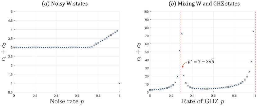
Fig 2: The optimal sampling overhead $c_{1}+c_{2}$ of virtual recovery for W state mixing with other quantum states. Panel (a) illustrates the case of virtual recovering a 3-qubit W state affected by a depolarizing channel of noise rate $p$; Panel (b) illustrates the case of virtual recovering $GW(p)$, a W state mixed with a GHZ state. At $p^{*}=7-3\sqrt{5}$, the mixed state is not a VQMC.

Sampling overhead of example states.

We investigate the sampling overhead of virtual recovery for different types of tripartite quantum states. Firstly, consider a W state under depolarizing noise as defined in Eq. (46). We present the sampling overhead of virtual recovery for $W(p)$ in Fig. 2 with $p\in[0,1]$. We observe that the sampling overhead of virtual recovery for $W(p)$ is $\log(c_{1}+c_{2})=\log 3$ when $0\leq p\lesssim 0.725$. There is a jump discontinuity at $p=1$, indicating that even with mixing the maximally mixed state with an extremely small amount of W state, the sampling overhead increases a lot. Secondly, consider the convex combination of a three-qubit W state and a GHZ state as defined in Example 2. The sampling overhead of virtual recovery for $GW(p)$ is depicted in Fig. 2 with $p\in[0,1]$. As stated in Example 2, we observe that the sampling overhead is infinity when $p^{*}=7-3\sqrt{5}$.

4 Approximate virtual quantum Markov chain

In the same spirit as the approximate quantum Markov chain, we study whether the properties of virtual quantum Markov chains are robust in this section. Note that the information we want to recover for a virtual quantum Markov chain is its measurement statistics with respect to any observable, and the recovery map is not completely positive. We herein introduce the $\varepsilon$-approximate virtual quantum Markov chain.

Definition 3 ($\varepsilon$-approximate virtual quantum Markov chain)

A tripartite quantum state $\rho_{ABC}\in{\cal D}(A\otimes B\otimes C)$ is called a $\varepsilon$-approximate virtual quantum Markov chain in order $A\leftrightarrow B\leftrightarrow C$ if

$$\min_{\mathscr{M}\in\text{\rm HPTP}(B,B\otimes C)}\left\|\mathscr{M}_{B\rightarrow BC}\circ\operatorname{Tr}_{C}(\rho_{ABC})-\rho_{ABC}\right\|_{1}=\varepsilon,$$ (116)

where $\mathscr{M}_{B\rightarrow BC}$ ranges over all HPTP maps.

Denote the optimal map in Eq. (116) as $\widetilde{\mathscr{M}}_{B\rightarrow BC}$ and $\widehat{\rho}_{ABC}=\mathscr{M}_{B\rightarrow BC}\circ\operatorname{Tr}_{C}(\rho_{ABC})$. Using a quasiprobability decomposition implementation for $\widetilde{\mathscr{M}}_{B\rightarrow BC}$, we can estimate the value of $\operatorname{Tr}(O\rho_{ABC})$ approximately for any possible observable $O$. Specifically, for any given observable $O$, we have

$$|\operatorname{Tr}(O\widehat{\rho}_{ABC})-\operatorname{Tr}(O\rho_{ABC})|\leq\|O\|_{\infty}\cdot\left\|\widehat{\rho}_{ABC}-\rho_{ABC}\right\|_{1}=\|O\|_{\infty}\cdot\varepsilon,$$ (117)

where the inequality is followed by Hölder’s inequality. The $\varepsilon$ actually corresponds to the approximate virtual recoverability of $\rho_{ABC}$. For any given tripartite quantum state $\rho_{ABC}$, its approximate virtual recoverability can be evaluated by the following SDPs.

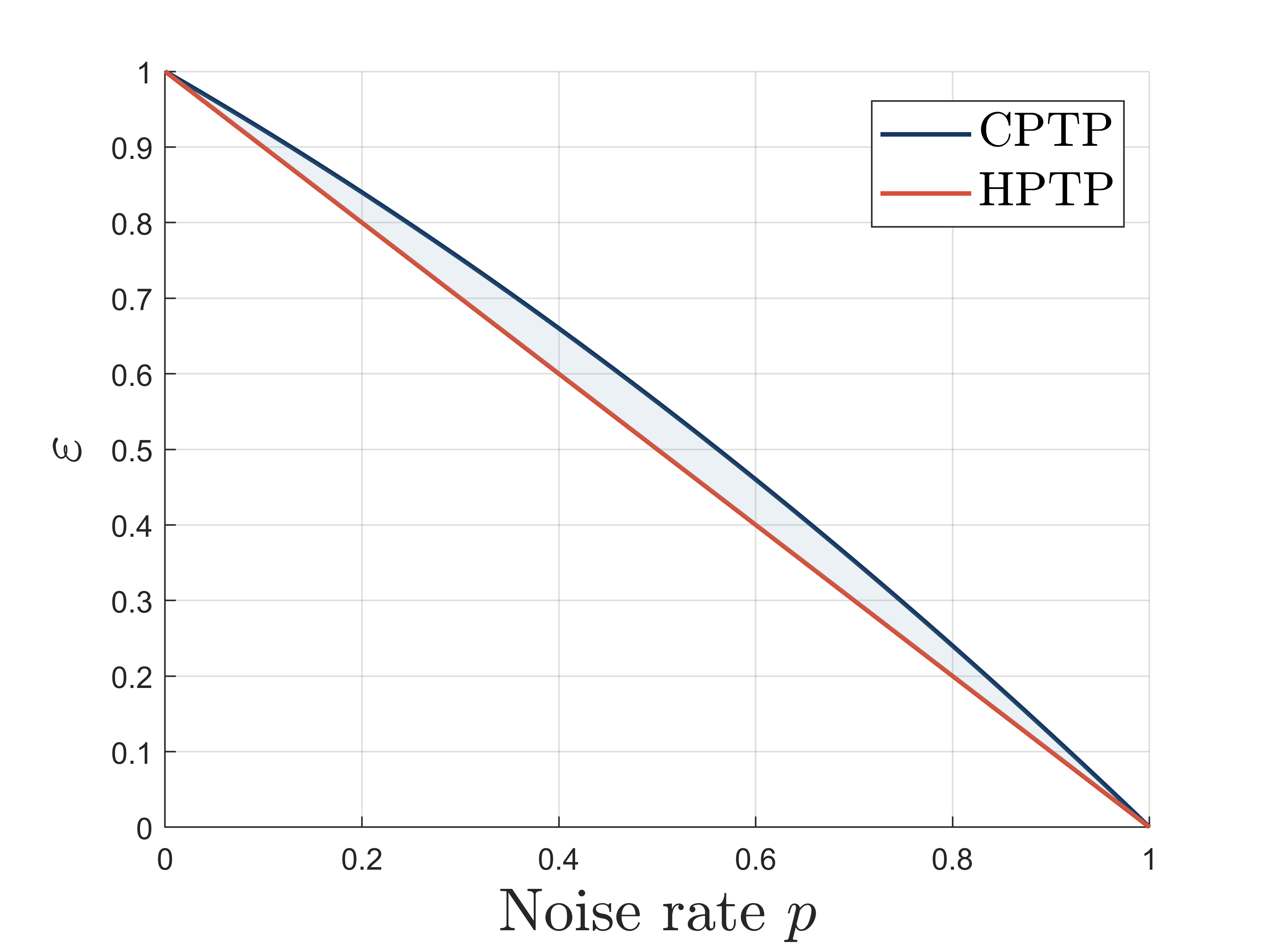
Fig 3: Comparison of $\varepsilon$ under CPTP and HPTP recovery maps. A 3-qubit GHZ state is affected by depolarizing channels with varying noise rates $p$. The dark blue and red curves illustrate the minimum $\varepsilon$ values assisted by CPTP and HPTP, respectively.

$$\begin{aligned} &\underline{\textbf{Primal Program}}\\ \min&\;\;\operatorname{Tr}S_{ABC}\\ {\rm s.t.}&\;\;\operatorname{Tr}_{B}(\rho_{AB}^{T_{B}}\otimes I_{B^{\prime}C})(I_{A}\otimes J_{BB^{\prime}C})=\sigma_{AB^{\prime}C},\\ &\;\;S_{ABC}\geq\rho_{ABC}-\sigma_{ABC},\\ &\;\;\operatorname{Tr}_{B^{\prime}C}J_{BB^{\prime}C}=I_{B},\\ \end{aligned}\quad\begin{aligned} &\underline{\textbf{Dual Program}}\\ \max&\;\operatorname{Tr}P_{B}+\operatorname{Tr}[R_{ABC}\rho_{ABC}]\\ {\rm s.t.}&\;\;\operatorname{Tr}_{A}(R_{AB^{\prime}C}\rho_{AB}^{T_{B}})=\tau_{BB^{\prime}C},\\ &\;\;P_{B}\otimes I_{B^{\prime}C}+\tau_{BB^{\prime}C}=0,\\ &\;\;R_{ABC}\leq I_{ABC}.\end{aligned}$$ (118)

The derivation of the dual SDP is in Appendix C. We consider a tripartite state $G(p)$ as defined in Eq. (46) and utilize SDPs in Eq. (118) to determine the approximate virtual recoverability of $G(p)$ with $p\in[0,1]$. Note that we can also utilize the primal SDP in Eq. (118) to calculate the minimum $\varepsilon$ when the recovery map $\mathscr{M}_{B\rightarrow BC}$ allowed is restricted to CPTP by simply adding a positivity constraint for $J_{BB^{\prime}C}$ ($J_{BB^{\prime}C}\geq 0$). We show the minimum $\varepsilon$ for $G(p)$ with different noise parameters $p$ in Fig. 3 where the red line corresponds to the value of Eq. (116) and the blue line corresponds to the case where $\mathscr{M}_{B\rightarrow BC}$ ranges over all quantum channels. We observe that HPTP maps can indeed offer improvement considering a general upper bound $\varepsilon\cdot\|O\|_{\infty}$ in Eq. (117) for the expectation value with respect to any observable.

5 Discussions

In this work, we introduce the concept of virtual quantum Markov chains, which allow for the recovery of global shadow information from subsystems through quantum operations and post-processing. Concerning the structure and distinctions between quantum Markov chains and their virtual counterparts, we present an algebraic characterization of virtual quantum Markov chains, establishing an easily verifiable criterion for a state to be a VQMC. Additionally, we propose a protocol for recovering shadow information involving the sampling of local quantum channels and classical post-processing. Through analysis of the sampling overhead via semidefinite programming, we uncover intriguing phenomena related to specific states. Furthermore, our work introduces the concept of approximate virtual quantum Markov chains, where shadow information with respect to any observable can be recovered approximately. We provide a characterization of approximate recoverability through semidefinite programming, offering insights into recovering shadow information for this extended class of quantum states. This work deepens our understanding of the boundaries of quantum Markovian dynamics, particularly in the context of recovering quantum states with respect to unknown observables.

Having firmly delineated the algebraic structure of virtual quantum Markov chains (VQMC), it naturally leads us to ask whether there exists an entropic characterization inspired by the close relationship between quantum Markov chains and conditional mutual information [1, 5]. Further investigation into the properties and applications of approximate VQMC presents a compelling avenue of research. Additionally, an intriguing direction worth pursuing involves the development of protocols akin to the Petz recovery map and universal recovery maps [14], but specifically tailored for VQMC. These paths of exploration could advance the understanding of the limits of recoverability in quantum information theory.

Appendix for
Virtual Quantum Markov Chains

Appendix A Remarks on Theorem 1

Here we provide a Remark on the main Theorem 1, and present that a classical Markov chain and a quantum Markov chain are both indeed included as virtual quantum Markov chains implied by Theorem 1.

Remark 1 Moreover for Theorem 1, for a given tripartite quantum state $\rho_{ABC}$, the following are equivalent:

• $\rho_{ABC}$ is a virtual quantum Markov chain in order $A\leftrightarrow B\leftrightarrow C$;

• $\ker{{\Theta_{B|A}}}\subseteq\ker{{\Theta_{BC|A}}}$;

• $\ker{{\Theta_{B|A}}}=\ker{{\Theta_{BC|A}}}$;

• there exists a linear map ${\cal M}$ satisfying $\forall\,i,j,\ \mathcal{M}\left(Q_{B}^{(ij)}\right)=Q_{BC}^{(ij)}$;

• there exists a HPTP map ${\cal M}$ satisfying $\forall\,i,j,\ \mathcal{M}\left(Q_{B}^{(ij)}\right)=Q_{BC}^{(ij)}$.

Proposition S1

If a tripartite quantum state $\rho_{ABC}$ is a quantum Markov chain in order $A\leftrightarrow B\leftrightarrow C$, then it is a virtual quantum Markov chain.

Proof.

Recall that $\rho_{ABC}$ is a quantum Markov chain if and only if system $B$ can be decomposed into a direct sum tensor product

$${\cal H}_{B}=\underset{t}{\bigoplus}{\cal H}^{(t)}_{b^{L}}\otimes{\cal H}^{(t)}_{b^{R}},\quad\text{s.t.}\>\rho_{ABC}=\underset{t}{\bigoplus}q_{t}\rho^{(t)}_{Ab^{L}}\otimes\rho^{(t)}_{b^{R}C},$$ (S1)

with states $\rho_{Ab^{L}_{j}}$ on $\mathcal{H}_{A}\otimes\mathcal{H}_{b^{L}_{j}}$ and $\rho_{b^{R}_{j}C}$ on ${\cal H}_{b^{R}_{j}}\otimes\mathcal{H}_{C}$ and a probability distribution $\{q_{t}\}$. If $\rho_{ABC}=\underset{t}{\bigoplus}q_{t}\rho^{(t)}_{Ab^{L}}\otimes\rho^{(t)}_{b^{R}C}$, we have

$$Q_{BC}^{(ij)} =\bigoplus_{t}q_{t}(\langle i|_{A}\otimes I_{b^{L}})\rho^{(t)}_{Ab^{L}}(|j\rangle_{A}\otimes I_{b^{R}})\otimes\rho^{(t)}_{b^{R}C},$$ (S2)

$$Q_{B}^{(ij)} =\bigoplus_{t}q_{t}(\langle i|_{A}\otimes I_{b^{L}})\rho^{(t)}_{Ab^{L}}(|j\rangle_{A}\otimes I_{b^{R}})\otimes\rho^{(t)}_{b^{R}}.$$

Thus, for any $\mathbf{c}\in\ker{{\Theta_{B|A}}}$ such that

$$\mathbf{0}=\sum_{ij}c_{ij}Q^{(ij)}_{B} =\sum_{ij}c_{ij}\bigoplus_{t}q_{t}(\langle i|_{A}\otimes I_{b^{L}})\rho^{(t)}_{Ab^{L}}(|j\rangle_{A}\otimes I_{b^{R}})\otimes\rho^{(t)}_{b^{R}}$$ (S3)

$$=\bigoplus_{t}q_{t}\left(\sum_{ij}c_{ij}(\langle i|_{A}\otimes I_{b^{L}})\rho^{(t)}_{Ab^{L}}(|j\rangle_{A}\otimes I_{b^{R}})\right)\otimes\rho^{(t)}_{b^{R}},$$

it follows that

$$\sum_{ij}c_{ij}(\langle i|_{A}\otimes I_{b^{L}})\rho^{(t)}_{Ab^{L}}(|j\rangle_{A}\otimes I_{b^{R}})=0.$$ (S4)

Hence we have

$$\sum_{ij}c_{ij}Q_{BC}^{(ij)} =\sum_{ij}c_{ij}\bigoplus_{t}q_{t}(\langle i|_{A}\otimes I_{b^{L}})\rho^{(t)}_{Ab^{L}}(|j\rangle_{A}\otimes I_{b^{R}})\otimes\rho^{(t)}_{b^{R}C}$$ (S5)

$$=\bigoplus_{t}q_{t}\left(\sum_{ij}c_{ij}(\langle i|_{A}\otimes I_{b^{L}})\rho^{(t)}_{Ab^{L}}(|j\rangle_{A}\otimes I_{b^{R}})\right)\otimes\rho^{(t)}_{b^{R}C}$$

$$=0,$$

which yields $\mathbf{c}\in\ker{{\Theta_{BC|A}}}$. Applying Theorem 1, we arrive at the conclusion.     $\sqcap$$\sqcup$

Proposition S2

If a tripartite classical state $\rho_{ABC}$ is a Markov chain in order $A\leftrightarrow B\leftrightarrow C$, then it is a virtual quantum Markov chain.

Proof.

For a classical state $\rho_{ABC}=\sum_{ijk}p_{ijk}|i\rangle\!\langle i|\otimes|j\rangle\!\langle j|\otimes|k\rangle\!\langle k|$, we have

$$Q_{BC}^{(ii)}=\sum_{jk}p_{ijk}|j\rangle\!\langle j|\otimes|k\rangle\!\langle k|,\quad Q_{B}^{(ii)}=\sum_{j}p_{ij}|j\rangle\!\langle j|,$$ (S6)

where $p_{ij}=\sum_{k}p_{ijk}$. Since $p_{ijk}=p_{ij}\cdot p_{jk}/p_{j}$ for a classical Markov chain. We have for any $\mathbf{c}\in\ker{{\Theta_{B|A}}}$, i.e., $\sum_{i}c_{i}p_{ij}=0,\forall j$, it follows

$$\sum_{i}c_{i}p_{ijk}=\frac{p_{jk}}{p_{j}}\sum_{i}c_{i}p_{ij}=0,\,\forall j,$$ (S7)

which means $\mathbf{c}\in\ker{{\Theta_{BC|A}}}$. By Theorem 1, we have $\rho_{ABC}$ is a virtual quantum Markov chain.     $\sqcap$$\sqcup$

Appendix B SDP for sampling overhead of virtual recovery

The primal SDP for the sampling overhead of the virtual recovery map of $\rho_{ABC}$ can be written as:

$$\min \;c_{1}+c_{2}$$ (S8a)

$${\rm s.t.} \;\;J_{1}\geq 0,J_{2}\geq 0,$$ (S8b)

$$\;\;J_{BB^{\prime}C}=J_{1}-J_{2},$$ (S8c)

$$\;\;\operatorname{Tr}_{B^{\prime}C}J_{1}=c_{1}I_{B},\operatorname{Tr}_{B^{\prime}C}J_{2}=c_{2}I_{B},$$ (S8d)

$$\;\;\operatorname{Tr}_{B}(\rho_{AB}^{T_{B}}\otimes I_{B^{\prime}C})(I_{A}\otimes J_{BB^{\prime}C})=\rho_{ABC}.$$ (S8e)

The Lagrange function of the primal problem is

$$L(M,N,K,c_{1},c_{2},J_{1},J_{2})$$ (S9)

$$= c_{1}+c_{2}+\langle M,\operatorname{Tr}_{B^{\prime}C}J_{1}-c_{1}I_{B}\rangle+\langle N,\operatorname{Tr}_{B^{\prime}C}J_{2}-c_{2}I_{B}\rangle$$

$$+\langle K,\rho_{ABC}-\operatorname{Tr}_{B}(\rho_{AB}^{T_{B}}\otimes I_{B^{\prime}C})(I_{A}\otimes J_{BB^{\prime}C})\rangle$$

$$= \operatorname{Tr}(K_{AB^{\prime}C}\rho_{AB^{\prime}C})+c_{1}(1-\operatorname{Tr}M)+c_{2}(1-\operatorname{Tr}N)$$

$$+\langle J_{1},M_{B}\otimes I_{B^{\prime}C}-\operatorname{Tr}_{A}[(K_{AB^{\prime}C}\otimes I_{B})(\rho_{AB}^{T_{B}}\otimes I_{B^{\prime}C})]\rangle$$

$$+\langle J_{2},N_{B}\otimes I_{B^{\prime}C}+\operatorname{Tr}_{A}[(K_{AB^{\prime}C}\otimes I_{B})(\rho_{AB}^{T_{B}}\otimes I_{B^{\prime}C})]\rangle,$$

where $M_{B},N_{B},K_{AB^{\prime}C}$ are Lagrange multipliers. The corresponding Lagrange dual function is

$$g(M,N,K)=\inf_{J_{1},J_{2}\geq 0}L(M,N,K,c_{1},c_{2},J_{1},J_{2}).$$ (S10)

Since $J_{1}\geq 0,J_{2}\geq 0$, it must hold that $\operatorname{Tr}M\leq 1,\operatorname{Tr}N\leq 1$ and

$$M_{B}\otimes I_{B^{\prime}C}-\operatorname{Tr}_{A}[(K_{AB^{\prime}C}\otimes I_{B})(\rho_{AB}^{T_{B}}\otimes I_{B^{\prime}C})] \geq 0,$$ (S11)

$$N_{B}\otimes I_{B^{\prime}C}+\operatorname{Tr}_{A}[(K_{AB^{\prime}C}\otimes I_{B})(\rho_{AB}^{T_{B}}\otimes I_{B^{\prime}C})] \geq 0.$$ (S12)

Thus the dual SDP is

$$\max_{M_{B},N_{B},K_{AB^{\prime}C}} \operatorname{Tr}[K_{AB^{\prime}C}\rho_{ABC}]$$ (S13)

$${\rm s.t.} \;\operatorname{Tr}M_{B}\leq 1,\operatorname{Tr}N_{B}\leq 1,$$

$$\;M_{B}\otimes I_{B^{\prime}C}-\operatorname{Tr}_{A}[(K_{AB^{\prime}C}\otimes I_{B})(\rho_{AB}^{T_{B}}\otimes I_{B^{\prime}C})]\geq 0,$$

$$\;N_{B}\otimes I_{B^{\prime}C}+\operatorname{Tr}_{A}[(K_{AB^{\prime}C}\otimes I_{B})(\rho_{AB}^{T_{B}}\otimes I_{B^{\prime}C})]\geq 0.$$

Appendix C SDP for approximate virtual recoverability

The primal SDP for approximate virtual recoverability can be written as:

$$\min_{S_{ABC}\geq 0,J_{BB^{\prime}C}} \operatorname{Tr}S_{ABC}$$ (S14)

$${\rm s.t.} \;\;S_{ABC}\geq\rho_{ABC}-\sigma_{ABC},$$

$$\;\;\operatorname{Tr}_{B}(\rho_{AB}^{T_{B}}\otimes I_{B^{\prime}C})(I_{A}\otimes J_{BB^{\prime}C})=\sigma_{AB^{\prime}C},$$

$$\;\;\operatorname{Tr}_{B^{\prime}C}J_{BB^{\prime}C}=I_{B}.$$

The Lagrange function of the primal problem is

$$L(P,R,S,J)$$ (S15)

$$= \operatorname{Tr}S_{ABC}+\operatorname{Tr}\{R_{ABC}[\rho_{ABC}-\operatorname{Tr}_{B}(\rho_{AB}^{T_{B}}\otimes I_{B^{\prime}C})(I_{A}\otimes J_{BB^{\prime}C})-S_{ABC}]\}$$

$$+\operatorname{Tr}[P_{B}(I_{B}-\operatorname{Tr}_{B^{\prime}C}J_{BB^{\prime}C})]$$

$$= \operatorname{Tr}P_{B}+\operatorname{Tr}[R_{ABC}\rho_{ABC}]+\operatorname{Tr}[S_{ABC}(I_{ABC}-R_{ABC})]$$

$$-\operatorname{Tr}\{J_{BB^{\prime}C}(P_{B}\otimes I_{B^{\prime}C}+\operatorname{Tr}_{A}[(R_{AB^{\prime}C}\otimes I_{B})(\rho_{AB}^{T_{B}}\otimes I_{B^{\prime}C})])\},$$

where $P_{B},R_{ABC}$ are Lagrange multipliers. $S_{ABC}\geq 0$ and $J_{BB^{\prime}C}\in\mathcal{L}^{\dagger}(\mathcal{H})$ respectively require

$$I_{ABC}-R_{ABC} \geq 0,$$ (S16)

$$P_{B}\otimes I_{B^{\prime}C}+\operatorname{Tr}_{A}[R_{AB^{\prime}C} \otimes I_{B}(\rho_{AB}^{T_{B}}\otimes I_{B^{\prime}C})]=0.$$

So the dual SDP is

$$\max_{R_{ABC}\geq 0,P_{B}} \;\operatorname{Tr}P_{B}+\operatorname{Tr}[R_{ABC}\rho_{ABC}]$$ (S17)

$${\rm s.t.} \;\;I_{ABC}\geq R_{ABC},$$

$$\;\;P_{B}\otimes I_{B^{\prime}C}+\operatorname{Tr}_{A}[(R_{AB^{\prime}C}\otimes I_{B})(\rho_{AB}^{T_{B}}\otimes I_{B^{\prime}C})]=0.$$

References

- [1] D. Petz, “Sufficient subalgebras and the relative entropy of states of a von Neumann algebra,” Communications in Mathematical Physics, vol. 105, no. 1, pp. 123–131, 1986.
- [2] D. Petz, “Sufficiency of channels over von Neumann algebras,” The Quarterly Journal of Mathematics, vol. 39, no. 1, pp. 97–108, 1988.
- [3] H. Barnum and E. Knill, “Reversing quantum dynamics with near-optimal quantum and classical fidelity,” Journal of Mathematical Physics, vol. 43, pp. 2097–2106, may 2002.
- [4] P. Hayden, R. Jozsa, D. Petz, and A. Winter, “Structure of states which satisfy strong subadditivity of quantum entropy with equality,” Communications in mathematical physics, vol. 246, no. 2, pp. 359–374, 2004.
- [5] O. Fawzi and R. Renner, “Quantum Conditional Mutual Information and Approximate Markov Chains,” Communications in Mathematical Physics, vol. 340, pp. 575–611, dec 2015.
- [6] D. Sutter, “Approximate quantum Markov chains,” arXiv preprint arXiv:1802.05477, 2018.
- [7] B. Ibinson, N. Linden, and A. Winter, “Robustness of Quantum Markov Chains,” Communications in Mathematical Physics, vol. 277, pp. 289–304, nov 2007.
- [8] F. G. S. L. Brandão, A. W. Harrow, J. Oppenheim, and S. Strelchuk, “Quantum Conditional Mutual Information, Reconstructed States, and State Redistribution,” Physical Review Letters, vol. 115, p. 050501, jul 2015.
- [9] M. Berta and M. Tomamichel, “The Fidelity of Recovery Is Multiplicative,” IEEE Transactions on Information Theory, vol. 62, pp. 1758–1763, apr 2016.
- [10] M. M. Wilde, “Recoverability in quantum information theory,” Proceedings of the Royal Society A: Mathematical, Physical and Engineering Science, vol. 471, p. 20150338, oct 2015.
- [11] L. Lami, S. Das, and M. M. Wilde, “Approximate reversal of quantum Gaussian dynamics,” Journal of Physics A: Mathematical and Theoretical, vol. 51, p. 125301, mar 2018.
- [12] K. P. Seshadreesan and M. M. Wilde, “Fidelity of recovery, squashed entanglement, and measurement recoverability,” Physical Review A, vol. 92, p. 042321, oct 2015.
- [13] D. Sutter and R. Renner, “Necessary Criterion for Approximate Recoverability,” Annales Henri Poincaré, vol. 19, pp. 3007–3029, oct 2018.
- [14] D. Sutter, O. Fawzi, and R. Renner, “Universal recovery map for approximate Markov chains,” Proceedings of the Royal Society A: Mathematical, Physical and Engineering Sciences, vol. 472, p. 20150623, feb 2016.
- [15] S. Aaronson, “Shadow tomography of quantum states,” in Proceedings of the 50th Annual ACM SIGACT Symposium on Theory of Computing - STOC 2018, (New York, New York, USA), pp. 325–338, ACM Press, nov 2018.
- [16] X. Zhao, B. Zhao, Z. Xia, and X. Wang, “Information recoverability of noisy quantum states,” Quantum, vol. 7, p. 978, apr 2023.
- [17] K. Temme, S. Bravyi, and J. M. Gambetta, “Error Mitigation for Short-Depth Quantum Circuits,” Physical Review Letters, vol. 119, p. 180509, nov 2017.
- [18] J. Jiang, K. Wang, and X. Wang, “Physical Implementability of Linear Maps and Its Application in Error Mitigation,” Quantum, vol. 5, p. 600, dec 2021.
- [19] C. Piveteau, D. Sutter, and S. Woerner, “Quasiprobability decompositions with reduced sampling overhead,” npj Quantum Information, vol. 8, p. 12, feb 2022.
- [20] X. Zhao, L. Zhang, B. Zhao, and X. Wang, “Power of quantum measurement in simulating unphysical operations,” arXiv preprint arXiv:2309.09963, 2023.
- [21] K. Mitarai and K. Fujii, “Overhead for simulating a non-local channel with local channels by quasiprobability sampling,” Quantum, vol. 5, p. 388, jan 2021.
- [22] C. Piveteau and D. Sutter, “Circuit knitting with classical communication,” IEEE Transactions on Information Theory, pp. 1–1, apr 2023.
- [23] X. Yuan, B. Regula, R. Takagi, and M. Gu, “Virtual quantum resource distillation,” arXiv preprint arXiv:2303.00955, mar 2023.
- [24] A. Elben, R. Kueng, H.-Y. R. Huang, R. van Bijnen, C. Kokail, M. Dalmonte, P. Calabrese, B. Kraus, J. Preskill, P. Zoller, and B. Vermersch, “Mixed-State Entanglement from Local Randomized Measurements,” Physical Review Letters, vol. 125, p. 200501, nov 2020.
- [25] K. Wang, Z. Song, X. Zhao, Z. Wang, and X. Wang, “Detecting and quantifying entanglement on near-term quantum devices,” npj Quantum Information, vol. 8, p. 52, dec 2022.
- [26] B. Regula, R. Takagi, and M. Gu, “Operational applications of the diamond norm and related measures in quantifying the non-physicality of quantum maps,” Quantum, vol. 5, p. 522, aug 2021.
- [27] H. Yao, X. Liu, C. Zhu, and X. Wang, “Optimal uni-local virtual quantum broadcasting,” arXiv preprint arXiv:2310.15156, pp. 1–11, oct 2023.
- [28] A. J. Parzygnat, J. Fullwood, F. Buscemi, and G. Chiribella, “Virtual quantum broadcasting,” arXiv preprint arXiv:2310.13049, pp. 1–14, oct 2023.
- [29] C. Piveteau, D. Sutter, S. Bravyi, J. M. Gambetta, and K. Temme, “Error Mitigation for Universal Gates on Encoded Qubits,” Physical Review Letters, vol. 127, p. 200505, nov 2021.
- [30] W. Dür, G. Vidal, and J. I. Cirac, “Three qubits can be entangled in two inequivalent ways,” Physical Review A, vol. 62, Nov. 2000.
- [31] M. Żukowski, A. Zeilinger, M. Horne, and H. Weinfurter, “Quest for ghz states,” Acta Physica Polonica A, vol. 93, no. 1, pp. 187–195, 1998.
- [32] H. Qin and Y. Dai, “Dynamic quantum secret sharing by using d-dimensional ghz state,” Quantum information processing, vol. 16, pp. 1–13, 2017.
- [33] T. Hwang, C. Hwang, and C. Tsai, “Quantum key distribution protocol using dense coding of three-qubit w state,” The European Physical Journal D, vol. 61, pp. 785–790, 2011.
- [34] C. F. Roos, M. Riebe, H. Haffner, W. Hansel, J. Benhelm, G. P. Lancaster, C. Becher, F. Schmidt-Kaler, and R. Blatt, “Control and measurement of three-qubit entangled states,” science, vol. 304, no. 5676, pp. 1478–1480, 2004.
- [35] S. P. Boyd and L. Vandenberghe, Convex optimization. Cambridge university press, 2004.
- [36] W. Hoeffding, The collected works of Wassily Hoeffding. Springer Science & Business Media, 2012.