Stochastic Optimal Control Matching

Abstract

Stochastic optimal control, which has the goal of driving the behavior of noisy systems, is broadly applicable in science, engineering and artificial intelligence. Our work introduces Stochastic Optimal Control Matching (SOCM), a novel Iterative Diffusion Optimization (IDO) technique for stochastic optimal control that stems from the same philosophy as the conditional score matching loss for diffusion models. That is, the control is learned via a least squares problem by trying to fit a matching vector field. The training loss, which is closely connected to the cross-entropy loss, is optimized with respect to both the control function and a family of reparameterization matrices which appear in the matching vector field. The optimization with respect to the reparameterization matrices aims at minimizing the variance of the matching vector field. Experimentally, our algorithm achieves lower error than all the existing IDO techniques for stochastic optimal control for three out of four control problems, in some cases by an order of magnitude. The key idea underlying SOCM is the path-wise reparameterization trick, a novel technique that is of independent interest, e.g., for generative modeling. The code can be found at https://github.com/facebookresearch/SOC-matching.

1 Introduction

Stochastic optimal control aims to drive the behavior of a noisy system in order to minimize a given cost. It has myriad applications in science and engineering: examples include the simulation of rare events in molecular dynamics [Hartmann et al., 2014, Hartmann and Schütte, 2012, Zhang et al., 2014, Holdijk et al., 2023], finance and economics [Pham, 2009, Fleming and Stein, 2004], stochastic filtering and data assimilation [Mitter, 1996, Reich, 2019], nonconvex optimization [Chaudhari et al., 2018], power systems and energy markets [Belloni et al., 2016, Powell and Meisel, 2016], and robotics [Theodorou et al., 2011, Gorodetsky et al., 2018]. Stochastic optimal has also been very impactful in neighboring fields such as mean-field games [Carmona et al., 2018], optimal transport [Villani, 2003, 2008], backward stochastic differential equations (BSDEs) [Carmona, 2016] and large deviations [Feng and Kurtz, 2006].

For continuous-time problems with low-dimensional state spaces, the standard approach to learn the optimal control is to solve the Hamilton-Jacobi-Bellman (HJB) partial differential equation (PDE) by gridding the space and using classical numerical methods. For high-dimensional problems, a large number of works parameterize the control using a neural network and train it applying a stochastic optimization algorithm on a loss function. These methods are known as Iterative Diffusion Optimization (IDO) techniques [Nüsken and Richter, 2021] (see Subsec. 2.2).

It is convenient to draw an analogy between stochastic optimal control and continuous normalizing flows (CNFs), which are a generative modeling technique where samples are generated by solving an ordinary differential equation (ODE) for which the vector field has been learned, initialized at a Gaussian sample. CNFs were introduced by Chen et al. [2018] (building on top of Rezende and Mohamed [2015]), and training them is similar to solving control problems because in both cases one needs to learn high-dimensional vector fields using neural networks, in continuous time.

The first algorithm developed to train normalizing flows was based on maximizing the likelihood of the generated samples [Chen et al., 2018, Sec. 4]. Obtaining the gradient of the maximum likelihood loss with respect to the vector field parameters requires backpropagating through the computation of the ODE trajectory, or equivalently, solving the adjoint ODE in parallel to the original ODE. Maximum likelihood CNFs (ML-CNFs) were superseded by diffusion models [Song and Ermon, 2019, Ho et al., 2020, Song et al., 2021] and flow-matching, a.k.a. stochastic interpolant, methods [Lipman et al., 2022, Albergo and Vanden-Eijnden, 2022, Pooladian et al., 2023, Albergo et al., 2023], which are currently the preferred algorithms to train CNFs. Aside from architectural improvements such as the UNet [Ronneberger et al., 2015], a potential reason for the success of diffusion and flow matching models is that their functional landscape is convex, unlike for ML-CNFs. Namely, vector fields are learned by solving least squares regression problems where the goal is to fit a random matching vector field. Convex functional landscapes in combination with overparameterized models and moderate gradient variance can yield very stable training dynamics and help achieve low error.

Returning to stochastic optimal control, one of the best-performing IDO techniques amounts to choosing the control objective (equation 1) as the training loss (see (12)). As in ML-CNFs, computing the gradient of this loss requires backpropagating through the computation of the trajectories of the SDE (2), or equivalently, using an adjoint method. The functional landscape of the loss is highly non-convex, and the method is prone to unstable training (see green curve in the bottom right plot of Figure 2). In light of this, a natural idea is to develop the analog of diffusion model losses for the stochastic optimal control problem, to obtain more stable training and lower error, and this is what we set out to do in our work. Our contributions are as follows:

• We introduce Stochastic Optimal Control Matching (SOCM), a novel IDO algorithm in which the control is learned by solving a least-squares regression problem where the goal is to fit a random matching vector field which depends on a family of reparameterization matrices that are also optimized.

• We derive a bias-variance decomposition of the SOCM loss (Prop. 2). The bias term is equal to an existing IDO loss: the cross-entropy loss, which shows that both algorithms have the same landscape in expectation. However, SOCM has an extra flexibility in the choice of reparameterization matrices, which affect only the variance. Hence, we propose optimizing the reparameterization matrices to reduce the variance of the SOCM objective.

• The key idea that underlies the SOCM algorithm is the path-wise reparameterization trick (Prop. 1), which is a novel technique for estimating gradients of an expectation of a functional of a random process with respect to its initial value. It is of independent interest and may be more generally applicable outside of the settings considered in this paper.

• We perform experiments on four different settings where we have access to the ground-truth control. For three of these, SOCM obtains a lower $L^{2}$ error with respect to the ground-truth control than all the existing IDO techniques, with around $10\times$ lower error than competing methods in some instances.

2 Framework

2.1 Setup and Preliminaries

Let $(\Omega,\mathcal{F},(\mathcal{F}_{t})_{t\geq 0},\mathcal{P})$ be a fixed filtered probability space on which is defined a Brownian motion $B=(B_{t})_{t\geq 0}$. We consider the control-affine problem

$$\textstyle\min_{u\in\mathcal{U}}\mathbb{E}\big{[}\int_{0}^{T}\big{(}\frac{1}{2}\|u(X^{u}_{t},t)\|^{2}+f(X^{u}_{t},t)\big{)}\,\mathrm{d}t+g(X^{u}_{T})\big{]},$$ (1)

where $$\textstyle\mathrm{d}X^{u}_{t}=(b(X^{u}_{t},t)+\sigma(t)u(X^{u}_{t},t))\,\mathrm{d}t+\sqrt{\lambda}\sigma(t)\mathrm{d}B_{t},\qquad X^{u}_{0}\sim p_{0}.$$ (2)

and where $X_{t}^{u}\in\mathbb{R}^{d}$ is the state, $u:\mathbb{R}^{d}\times[0,T]$ is the feedback control and belongs to the set of admissible controls $\mathcal{U}$, $f:\mathbb{R}^{d}\times[0,T]\to\mathbb{R}$ is the state cost, $g:\mathbb{R}^{d}\to\mathbb{R}$ is the terminal cost, $b:\mathbb{R}^{d}\times[0,T]\to\mathbb{R}^{d}$ is the base drift, and $\sigma:[0,T]\to\mathbb{R}^{d\times d}$ is the invertible covariance matrix and $\lambda\in(0,+\infty)$ is the noise level. In App. A we formally define the set $\mathcal{U}$ of admissible controls and describe the regularity assumptions needed on the control functions. In the remainder of the section we introduce relevant concepts in stochastic optimal control; we provide the most relevant proofs in App. B and refer the reader to Oksendal [2013, Chap. 11] and Nüsken and Richter [2021, Sec. 2] for a similar, more extensive treatment.

Cost functional and value function

The cost functional for the control $u$, point $x$ and time $t$ is defined as $J(u;x,t):=\mathbb{E}\big{[}\int_{t}^{T}\big{(}\frac{1}{2}\|u_{s}(X^{u}_{s})\|^{2}+f_{s}(X^{u}_{s})\big{)}\,\mathrm{d}t+g(X^{u}_{T})\big{|}X^{u}_{t}=x\big{]}.$ That is, the cost functional is the expected value of the control objective restricted to the times $[t,T]$ with the initial value $x$ at time $t$. The value function or optimal cost-to-go at a point $x$ and time $t$ is defined as the minimum value of the cost functional across all possible controls:

$$\textstyle V(x,t):=\inf_{u\in\mathcal{U}}J(u;x,t).$$ (3)

Hamilton-Jacobi-Bellman equation and optimal control

If we define the infinitesimal generator $L:=\frac{\lambda}{2}\sum_{i,j=1}^{d}(\sigma\sigma^{\top})_{ij}(t)\partial_{x_{i}}\partial_{x_{j}}+\sum_{i=1}^{d}b_{i}(x,t)\partial_{x_{i}}$, the value function solves the following Hamilton-Jacobi-Bellman (HJB) partial differential equation:

$$\textstyle\begin{split}\textstyle&\textstyle(\partial_{t}+L)V(x,t)-\frac{1}{2}\|(\sigma^{\top}\nabla V)(x,t)\|^{2}+f(x,t)=0,\\ \textstyle&\textstyle V(x,T)=g(x).\end{split}$$ (4)

The verification theorem [Pavliotis, 2014, Sec. 2.3] states that if a function $V$ solves the HJB equation above and has certain regularity conditions, then $V$ is the value function (3) of the problem (1)-(2). An implication of the verification theorem is that for every $u\in\mathcal{U}$,

$$\textstyle V(x,t)+\mathbb{E}\big{[}\frac{1}{2}\int_{t}^{T}\|\sigma^{\top}\nabla V+u\|^{2}(X^{u}_{s},s)\,\mathrm{d}s\,\big{|}\,X^{u}_{t}=x\big{]}=J(u,x,t).$$ (5)

In particular, this implies that the unique optimal control is given in terms of the value function as $u^{*}(x,t)=-\sigma(t)^{\top}\nabla V(x,t)$. Equation (5) can be deduced by integrating the HJB equation (LABEL:eq:HJB_setup) over $[t,T]$, and taking the conditional expectation with respect to $X^{u}_{t}=x$. We include the proof of (5) in App. B for completeness.

A pair of forward and backward SDEs (FBSDEs)

Consider the pair of SDEs

$$\textstyle\mathrm{d}X_{t} \textstyle=b(X_{t},t)\,\mathrm{d}t+\sqrt{\lambda}\sigma(X_{t},t)\mathrm{d}B_{t},\qquad X_{0}\sim p_{0},$$ (6)

$$\textstyle\mathrm{d}Y_{t} \textstyle=(-f(X_{t},t)+\frac{1}{2}\|Z_{t}\|^{2})\,\mathrm{d}t+\sqrt{\lambda}\langle Z_{t},\mathrm{d}B_{t}\rangle,\qquad Y_{T}=g(X_{T}).$$ (7)

where $Y:\Omega\times[0,T]\to\mathbb{R}$ and $Z:\Omega\times[0,T]\to\mathbb{R}^{d}$ are progressively measurable random processes. It turns out that $Y_{t}$ and $Z_{t}$ defined as $Y_{t}:=V(X_{t},t)$ and $Z_{t}:=\sigma(t)^{\top}\nabla V(X_{t},t)=-u^{*}(X_{t},t)$ satisfy (7). We include the proof in App. B for completeness.

An analytic expression for the value function

From the forward-backward equations (6)-(7), one can derive a closed-form expression for the value function $V$:

$$\textstyle V(x,t)=-\lambda\log\mathbb{E}\big{[}\exp\big{(}-\lambda^{-1}\int_{t}^{T}f(X_{s},s)\,\mathrm{d}s-\lambda^{-1}g(X_{T})\big{)}\big{|}X_{t}=x\big{]},$$ (8)

where $X_{t}$ is the solution of the uncontrolled SDE (6). This is a classical result, but we still include its proof in App. B. Given that $u^{*}(x,t)=-\sigma(t)^{\top}\nabla V(x,t)$, an immediate, yet important, consequence of (8) is the following representation of the optimal control:

Lemma 1 (Path-integral representation of the optimal control [Kappen, 2005]).

$$\textstyle u^{*}(x,t)\!=\!\lambda\sigma(t)^{\top}\nabla_{x}\log\mathbb{E}\big{[}\exp\big{(}-\lambda^{-1}\int_{t}^{T}f(X_{s},s)\,\mathrm{d}s-\lambda^{-1}g(X_{T})\big{)}\big{|}X_{t}=x\big{]}~{}.$$ (9)

Remark that the right-hand side of this equation involves the gradient of logarithm of a conditional expectation. This is reminiscent of the vector fields that are learned when training diffusion models or flow matching algorithms. For example, the target vector field for variance-exploding score-based diffusion loss [Song et al., 2021] can be expressed as $\nabla_{x}\log p_{t}(x)=\nabla_{x}\log\mathbb{E}_{Y\sim p_{\mathrm{data}}}[\frac{\exp(-\|x-Y\|^{2}/(2\sigma_{t}^{2}))}{(2\pi\sigma_{t}^{2})^{d/2}}]$. Note, however, that in (9) the gradient is taken with respect to the initial condition of the process, which requires the development of novel techniques.

Conditioned diffusions

Let $\mathcal{C}=C([0,T];\mathbb{R}^{d})$ be the Wiener space of continuous functions from $[0,T]$ to $\mathbb{R}^{d}$ equipped with the supremum norm, and let $\mathcal{P}(\mathcal{C})$ be the space of Borel probability measures over $\mathcal{C}$. For each control $u\in\mathcal{U}$, the controlled process in equation (2) induces a probability measure in $\mathcal{P}(\mathcal{C})$, as the law of the paths $X_{t}^{u}$, which we refer to as $\mathbb{P}^{u}$. We let $\mathbb{P}$ be the probability measure induced by the uncontrolled process (6), and define the work functional

$$\textstyle\mathcal{W}(X,t):=\int_{t}^{T}f(X_{s},s)\,\mathrm{d}s+g(X_{T}).$$ (10)

It turns out (4 in App. B) that the Radon-Nikodym derivative $\frac{d\mathbb{P}^{u^{*}}}{d\mathbb{P}}$ satisfies $\frac{d\mathbb{P}^{u^{*}}}{d\mathbb{P}}(X)=\exp\big{(}\lambda^{-1}\big{(}V(X_{0},0)-\mathcal{W}(X,0)\big{)}\big{)}$. Also, a straight-forward application of the Girsanov theorem for SDEs (Cor. 1) shows that

$$\textstyle\frac{d\mathbb{P}^{u}}{d\mathbb{P}^{u^{*}}}(X^{u^{*}})\!=\!\exp\big{(}\!-\!\lambda^{-1/2}\int_{0}^{T}\langle u^{*}(X^{u^{*}}_{t},t)\!-\!u(X^{u^{*}}_{t},t),\mathrm{d}B_{t}\rangle\!-\!\frac{\lambda^{-1}}{2}\int_{0}^{T}\|u^{*}(X^{u^{*}}_{t},t)\!-\!u(X^{u^{*}}_{t},t)\|^{2}\,\mathrm{d}t\big{)},$$ (11)

which means that the only control $u\in\mathcal{U}$ such that $\mathbb{P}^{u}=\mathbb{P}^{u^{*}}$ is the optimal control itself. Such changes of process are the basic tools to design IDO losses, and we leverage them as well.

2.2 Existing approaches and related work

Low-dimensional case: solving the HJB equation

For low-dimensional control problems ($d\leq 3$), it is possible to grid the domain and use a numerical PDE solver to find a solution to the HJB equation (LABEL:eq:HJB_setup). The main approaches include finite difference methods [Bonnans et al., 2004, Ma and Ma, 2020, Baňas et al., 2022], which approximate the derivatives and gradients of the value function using finite differences, finite element methods [Jensen and Smears, 2013], which involve restricting the solution to domain-dependent function spaces, and semi-Lagrangian schemes [Debrabant and Jakobsen, 2013, Carlini et al., 2020, Calzola et al., 2022], which trace back characteristics and have better stability than finite difference methods. See Greif [2017] for an overview on these techniques, and Baňas et al. [2022] for a comparison between them. Hutzenthaler et al. [2016] introduced the multilevel Picard method, which leverages the Feynman-Kac and the Bismut-Elworthy-Li formulas to beat the curse of dimensionality in some settings [Beck et al., 2019, Hutzenthaler et al., 2019, 2018, Hutzenthaler and Kruse, 2020].

High dimensional methods leveraging FBSDEs

The FBSDE formulation in equations (6)-(7) has given rise to multiple methods to learn controls. One such approach is least-squares Monte Carlo (see Pham [2009, Chapter 3] and Gobet [2016] for an introduction, and Gobet et al. [2005], Zhang et al. [2004] for an extensive analysis), where trajectories from the forward process (6) are sampled, and then regression problems are solved backwards in time to estimate the expected future cost in the spirit of dynamic programming. A second method that exploits FBSDEs was proposed by E et al. [2017], Han et al. [2018]. They parameterize the control using a neural network $u_{\theta}$, and use stochastic gradient algorithms to minimize the loss $\mathcal{L}(u_{\theta},y_{0})=\mathbb{E}[(Y_{T}(y_{0},u_{\theta})-g(X_{T}))^{2}]$, where $Y_{T}(y_{0},u_{\theta})$ is the process in (7) with initial condition $y_{0}$ and control $u_{\theta}$. This algorithm can be seen as a shooting method, where the initial condition and the control are learned to match the terminal condition. Multiple recent works have combined neural networks with FBSDE Monte Carlo methods for parabolic and elliptic PDEs [Beck et al., 2018, Chan-Wai-Nam et al., 2019, Zhou et al., 2021], control [Becker et al., 2019, Hartmann et al., 2019], multi-agent games [Han and Hu, 2020, Carmona and Laurière, 2021, 2022]; see E et al. [2021] for a more comprehensive review.

Many of the methods referenced above and some additional ones can be seen from a common perspective using controlled diffusions. As observed in equation (11), the key idea is that learning the optimal control is equivalent to finding a control $u$ such that the induced probability measure $\mathbb{P}^{u}$ on paths is equal to the probability measure $\mathbb{P}^{u^{*}}$ for the optimal control. In the paragraphs below we cover several loss that fall into this framework. All the losses below can be optimized using a common algorithmic framework, which we describe in Algorithm 1. For more details, we refer the reader to Nüsken and Richter [2021], which introduced this perspective and named such methods Iterative Diffusion Optimization (IDO) techniques. For simplicity, we introduce the losses for the setting in which the initial distribution $p_{0}$ is concentrated at a single point $x_{\mathrm{init}}$; we cover the general setting in App. B.

Input: State cost $f(x,t)$, terminal cost $g(x)$, covariance matrix $\sigma(t)$, base drift $b(x,t)$, noise level $\lambda$, number of iterations $N$, batch size $m$, number of time steps $K$, initial control parameters $\theta_{0}$, loss $\mathcal{L}\in\{\mathcal{L}_{\mathrm{Adj}}\eqref{eq:L_RE},\mathcal{L}_{\mathrm{CE}}\eqref{eq:L_CE},\mathcal{L}_{\mathrm{Var}_{v}}\eqref{eq:variance_loss},\mathcal{L}_{\mathrm{Var}_{v}}^{\mathrm{log}}\eqref{eq:log_variance_loss},\mathcal{L}_{\mathrm{Mom}_{v}}\eqref{eq:moment_loss}\}$

1 for $n\in\{0,\dots,N-1\}$ do

2       Simulate $m$ trajectories of the process $X^{v}$ controlled by $v=u_{\theta_{n}}$, e.g., using Euler-Maruyama updates

3      if $\mathcal{L}\neq\mathcal{L}_{\mathrm{Adj}}$ then detach the $m$ trajectories from the computational graph, so that gradients do not backpropagate;

4      

5      Using the $m$ trajectories, compute an $m$-sample Monte Carlo approximation $\hat{\mathcal{L}}(u_{\theta_{n}})$ of the loss $\mathcal{L}(u_{\theta_{n}})$

6      Compute the gradients $\nabla_{\theta}\hat{\mathcal{L}}(u_{\theta_{n}})$ of $\hat{\mathcal{L}}(u_{\theta_{n}})$ w.r.t. $\theta_{n}$

7      Obtain $\theta_{n+1}$ with via an Adam update on $\theta_{n}$ (or another stochastic algorithm)

8 end for

Output: Learned control $u_{\theta_{N}}$

Algorithm 1 Iterative Diffusion Optimization (IDO) algorithms for stochastic optimal control

The relative entropy loss and the adjoint method

The relative entropy loss is defined as the Kullback-Leibler divergence between $\mathbb{P}^{u}$ and $\mathbb{P}^{u^{*}}$: $\mathbb{E}_{\mathbb{P}^{u}}[\log\frac{d\mathbb{P}^{u}}{d\mathbb{P}^{u^{*}}}]$. Upon removing constant terms and factors, this loss is equivalent to (see 5 in App. B, or Hartmann and Schütte [2012], Kappen et al. [2012]):

$$\textstyle\mathcal{L}_{\mathrm{Adj}}(u):=\mathbb{E}\big{[}\int_{0}^{T}\big{(}\frac{1}{2}\|u(X^{u}_{t},t)\|^{2}+f(X^{u}_{t},t)\big{)}\,\mathrm{d}t+g(X^{u}_{T})\big{]}.$$ (12)

This is exactly the control objective in (1). This connection has been studied extensively [Bierkens and Kappen, 2014, Gómez et al., 2014, Hartmann and Schütte, 2012, Kappen et al., 2012, Rawlik et al., 2013]. Hence, the relative entropy loss is a very natural one, and is widely used; see Onken et al. [2023], Zhang and Chen [2022] for some examples on multiagent systems and sampling.

Solving optimization problems of the form (12) has a long history that dates back to Pontryagin [1962]. Note that $\mathcal{L}_{\mathrm{Adj}}(u)$ depends on $u$ both explicitly, and implicitly through the process $X^{u}$. To compute the gradient $\nabla_{\theta}\hat{\mathcal{L}}_{\mathrm{Adj}}(u_{\theta_{n}})$ of a Monte Carlo approximation $\hat{\mathcal{L}}_{\mathrm{Adj}}(u_{\theta_{n}})$ of $\mathcal{L}_{\mathrm{Adj}}(u_{\theta_{n}})$ as required by Algorithm 1, we need to backpropagate through the simulation of the $m$ trajectories, which is why we do not detach them from the computational graph. One can alternatively compute the gradient $\nabla_{\theta}\hat{\mathcal{L}}_{\mathrm{Adj}}(u_{\theta_{n}})$ by explicitly solving an ODE, a technique which is known as the adjoint method. The adjoint method was introduced by Pontryagin [1962], popularized in deep learning by Chen et al. [2018], and further developed for SDEs in Li et al. [2020].

The cross-entropy loss

The cross-entropy loss is defined as the Kullback-Leibler divergence between $\mathbb{P}^{u^{*}}$ and $\mathbb{P}^{u}$, i.e., flipping the order of the two measures: $\mathbb{E}_{\mathbb{P}^{u^{*}}}[\log\frac{d\mathbb{P}^{u^{*}}}{d\mathbb{P}^{u}}]$. For an arbitrary $v\in\mathcal{U}$, this loss is equivalent to the following one (see Prop. 3(i) in App. B):

$$\textstyle\begin{split}\textstyle\mathcal{L}_{\mathrm{CE}}(u)&\textstyle:=\mathbb{E}\big{[}\big{(}\!-\!\lambda^{-1/2}\int_{0}^{T}\langle u(X^{v}_{t},t),\mathrm{d}B_{t}\rangle\!-\!\lambda^{-1}\int_{0}^{T}\langle u(X^{v}_{t},t),v(X^{v}_{t},t)\rangle\,\mathrm{d}t\!+\!\frac{\lambda^{-1}}{2}\int_{0}^{T}\|u(X^{v}_{t},t)\|^{2}\,\mathrm{d}t\big{)}\\ \textstyle&\textstyle\qquad\times\exp\big{(}-\lambda^{-1}\mathcal{W}(X^{v},0)\!-\!\lambda^{-1/2}\int_{0}^{T}\langle v(X^{v}_{t},t),\mathrm{d}B_{t}\rangle\!-\!\frac{\lambda^{-1}}{2}\int_{0}^{T}\|v(X^{v}_{t},t)\|^{2}\,\mathrm{d}t\big{)}\big{]}.\end{split}$$ (13)

The cross-entropy loss has a rich literature [Hartmann et al., 2017, Kappen and Ruiz, 2016, Rubinstein and Kroese, 2013, Zhang et al., 2014] and has been recently used in applications such as molecular dynamics [Holdijk et al., 2023].

Furthermore, we note that the cross-entropy loss can be significantly simplified and written in terms of the $L^{2}$ error of the control $u$ with respect to the optimal control $u^{*}$:

Lemma 2 (Cross-entropy loss in terms of control $L^{2}$ error).

$$\textstyle\mathcal{L}_{\mathrm{CE}}(u) \textstyle=\frac{\lambda^{-1}}{2}\mathbb{E}\big{[}\int_{0}^{T}\|u^{*}(X^{u^{*}}_{t},t)-u(X^{u^{*}}_{t},t)\|^{2}\,\mathrm{d}t\exp\big{(}-\lambda^{-1}V(X^{u^{*}}_{0},0)\big{)}\big{]}~{}.$$ (14)

This characterization, which is proven in Prop. 3(ii) in App. B, is relevant for us because a similar one can be written for the loss that we propose (see Prop. 2).

Variance and log-variance losses

For an arbitrary $v\in\mathcal{U}$, the variance and the log-variance losses are defined as $\tilde{\mathcal{L}}_{\mathrm{Var}_{v}}(u)=\mathrm{Var}_{\mathbb{P}^{v}}(\frac{\mathrm{d}\mathbb{P}^{u^{*}}}{\mathrm{d}\mathbb{P}^{u}})$ and $\tilde{\mathcal{L}}_{\mathrm{Var}_{v}}^{\mathrm{log}}(u)=\mathrm{Var}_{\mathbb{P}^{v}}(\log\frac{\mathrm{d}\mathbb{P}^{u^{*}}}{\mathrm{d}\mathbb{P}^{u}})$ whenever $\mathbb{E}_{\mathbb{P}^{v}}|\frac{\mathrm{d}\mathbb{P}^{u^{*}}}{\mathrm{d}\mathbb{P}^{u}}|<+\infty$ and $\mathbb{E}_{\mathbb{P}^{v}}|\log\frac{d\mathbb{P}^{u^{*}}}{d\mathbb{P}^{u}}|<+\infty$, respectively. Define

$$\textstyle\begin{split}\textstyle\tilde{Y}_{T}^{u,v}&\textstyle=-\lambda^{-1}\int_{0}^{T}\langle u(X^{v}_{t},t),v(X^{v}_{t},t)\rangle\,\mathrm{d}t-\lambda^{-1}\int_{0}^{T}f(X^{v}_{t},t)\,\mathrm{d}t-\lambda^{-1/2}\int_{0}^{T}\langle u(X^{v}_{t},t),\mathrm{d}B_{t}\rangle\\ \textstyle&\textstyle\qquad+\frac{\lambda^{-1}}{2}\int_{0}^{T}\|u(X^{v}_{t},t)\|^{2}\,\mathrm{d}t.\end{split}$$ (15)

Then, $\tilde{\mathcal{L}}_{\mathrm{Var}_{v}}$ and $\tilde{\mathcal{L}}_{\mathrm{Var}_{v}}^{\mathrm{log}}$ are equivalent, respectively, to the following losses (see 6):

$$\mathcal{L}_{\mathrm{Var}_{v}}(u) :=\mathrm{Var}\big{(}\exp\big{(}\tilde{Y}^{u,v}_{T}-\lambda^{-1}g(X^{v}_{T})\big{)}\big{)},$$ (16)

$$\mathcal{L}^{\mathrm{log}}_{\mathrm{Var}_{v}}(u) :=\mathrm{Var}\big{(}\tilde{Y}^{u,v}_{T}-\lambda^{-1}g(X^{v}_{T})\big{)},$$ (17)

The variance and log-variance losses were introduced by Nüsken and Richter [2021]. Unlike for the cross-entropy loss, the choice of the control $v$ does lead to different losses. When using $\mathcal{L}_{\mathrm{Var}_{v}}$ or $\mathcal{L}^{\mathrm{log}}_{\mathrm{Var}_{v}}$ in Algorithm 1, the variance is computed across the $m$ trajectories in each batch.

Moment loss

For an arbitrary $v\in\mathcal{U}$, the moment loss is defined as

$$\mathcal{L}_{\mathrm{Mom}_{v}}(u,y_{0})=\mathbb{E}[(\tilde{Y}^{u,v}_{T}+y_{0}-\lambda^{-1}g(X^{v}_{T}))^{2}],$$ (18)

where $\tilde{Y}^{u,v}_{T}$ is defined in (15). Note the similarity with the log-variance loss (17); the optimal value of $y_{0}$ for a fixed $u$ is $y_{0}^{*}=\mathbb{E}[\lambda^{-1}g(X^{v}_{T})-\tilde{Y}^{u,v}_{T}]$, and plugging this into (18) yields exactly the log-variance loss. The moment loss was introduced by Hartmann et al. [2019, Section III.B], and it is a generalization of the FBSDE method pioneered by E et al. [2017], Han et al. [2018] and referenced earlier in this subsection. In fact, the original method corresponds to setting $v=0$.

3 Stochastic Optimal Control Matching

In this section we present our loss, Stochastic Optimal Control Matching (SOCM). The corresponding method, which we describe in Algorithm 2, falls into the class of IDO techniques described in Subsec. 2.2. The general idea is to leverage the analytic expression of $u^{*}$ in 1 to write a least squares loss for $u$, and the main challenge is to reexpress the gradient of a conditional expectation with respect to the initial condition of the process. We do that using a novel technique which introduces certain arbitrary matrix-valued functions $M_{t}$, that we also optimize.

Theorem 1 (SOCM loss).

For each $t\in[0,T]$, let $M_{t}:[t,T]\to\mathbb{R}^{d\times d}$ be an arbitrary matrix-valued differentiable function such that $M_{t}(t)=\mathrm{Id}$. Let $v\in\mathcal{U}$ be an arbitrary control. Let $\mathcal{L}_{\mathrm{SOCM}}:L^{2}(\mathbb{R}^{d}\times[0,T];\mathbb{R}^{d})\times L^{2}([0,T]^{2};\mathbb{R}^{d\times d})\to\mathbb{R}$ be the loss function defined as

$$\textstyle\begin{split}\textstyle\mathcal{L}_{\mathrm{SOCM}}(u,M)&\textstyle:=\mathbb{E}\big{[}\frac{1}{T}\int_{0}^{T}\big{\|}u(X^{v}_{t},t)-w(t,v,X^{v},B,M_{t})\big{\|}^{2}\,\mathrm{d}t\times\alpha(v,X^{v},B)\big{]}~{},\end{split}$$ (19)

where $X^{v}$ is the process controlled by $v$ (i.e., $dX_{t}=(b(X_{t},t)+\sigma(t)v(X_{t},t))\,\mathrm{d}t+\sqrt{\lambda}\sigma(X_{t},t)\,\mathrm{d}B_{t}$ and $X_{0}\sim p_{0}$), and

$$\textstyle w(t,v,X^{v},B,M_{t}) \textstyle=\sigma(t)^{\top}\big{(}-\int_{t}^{T}M_{t}(s)\nabla_{x}f(X^{v}_{s},s)\,\mathrm{d}s-M_{t}(T)\nabla g(X^{v}_{T})$$ (20)

$$\textstyle\quad+\int_{t}^{T}(M_{t}(s)\nabla_{x}b(X^{v}_{s},s)-\partial_{s}M_{t}(s))(\sigma_{s}^{-1})^{\top}(X^{v}_{s},s)v(X^{v}_{s},s)\,\mathrm{d}s$$ (21)

$$\textstyle\quad+\lambda^{1/2}\int_{t}^{T}(M_{t}(s)\nabla_{x}b(X^{v}_{s},s)-\partial_{s}M_{t}(s))(\sigma_{s}^{-1})^{\top}(X^{v}_{s},s)\mathrm{d}B_{s}\big{)},$$ (22)

$$\textstyle\alpha(v,X^{v},B) \textstyle=\exp\big{(}-\lambda^{-1}\int_{0}^{T}f(X^{v}_{t},t)\,\mathrm{d}s-\lambda^{-1}g(X^{v}_{T})$$ (23)

$$\textstyle\qquad\qquad-\lambda^{-1/2}\int_{0}^{T}\langle v(X^{v}_{t},t),\mathrm{d}B_{t}\rangle-\frac{\lambda^{-1}}{2}\int_{0}^{T}\|v(X^{v}_{t},t)\|^{2}\,\mathrm{d}t\big{)}.$$ (24)

$\mathcal{L}_{\mathrm{SOCM}}$ has a unique optimum $(u^{*},M^{*})$, where $u^{*}$ is the optimal control.

We refer to $M={(M_{t})}_{t\in[0,T]}$ as the family of reparametrization matrices, to the random vector field $w$ as the matching vector field, and to $\alpha$ as the importance weight. We present a proof sketch of Thm. 1; the full proofs for all the results in this section are in App. C.

Proof sketch of Thm. 1

Recall that the optimal control is of the form $u^{*}(x,t)=-\sigma(t)^{\top}\nabla V(x,t)$. Let $X$ be the uncontrolled process (6). Consider the loss

$$\textstyle\tilde{\mathcal{L}}(u) \textstyle=\mathbb{E}\big{[}\frac{1}{T}\int_{0}^{T}\big{\|}u(X_{t},t)-u^{*}(X_{t},t)\big{\|}^{2}\,\mathrm{d}t\,\exp\big{(}-\lambda^{-1}\int_{0}^{T}f(X_{t},t)\,\mathrm{d}t-\lambda^{-1}g(X_{T})\big{)}\big{]}$$ (25)

$$\textstyle=\mathbb{E}\big{[}\frac{1}{T}\int_{0}^{T}\big{(}\big{\|}u(X_{t},t)\big{\|}^{2}-2\langle u(X_{t},t),u^{*}(X_{t},t)\rangle+\|u^{*}(X_{t},t)\big{\|}^{2}\big{)}\,\mathrm{d}t$$ (26)

$$\textstyle\qquad\qquad\times\exp\big{(}-\lambda^{-1}\int_{0}^{T}f(X_{t},t)\,\mathrm{d}t-\lambda^{-1}g(X_{T})\big{)}\big{]}.$$ (27)

Clearly, the only optimum of this loss is $u^{*}$. Using the analytic expression of $u^{*}$ in 1, the cross-term can be rewritten as (see 7 in App. C):

$$\textstyle\begin{split}\textstyle&\textstyle\mathbb{E}\big{[}\frac{1}{T}\int_{0}^{T}\langle u(X_{t},t),u^{*}(X_{t},t)\rangle\,\mathrm{d}t\,\exp\big{(}-\lambda^{-1}\int_{0}^{T}f(X_{t},t)\,\mathrm{d}t-\lambda^{-1}g(X_{T})\big{)}\big{]}\\ \textstyle&\textstyle=-\lambda\mathbb{E}\big{[}\frac{1}{T}\int_{0}^{T}\big{\langle}u(X_{t},t),\sigma(t)^{\top}\nabla_{x}\mathbb{E}\big{[}\exp\big{(}-\lambda^{-1}\int_{t}^{T}f(X_{s},s)\,\mathrm{d}s-\lambda^{-1}g(X_{T})\big{)}\big{|}X_{t}=x\big{]}\big{\rangle}\,\mathrm{d}t\\ \textstyle&\textstyle\qquad\qquad\times\exp\big{(}-\lambda^{-1}\int_{0}^{t}f(X_{s},s)\,\mathrm{d}s\big{)}\big{]}.\end{split}$$ (28)

It remains to evaluate the conditional expectation $\nabla_{x}\mathbb{E}\big{[}\exp\big{(}-\lambda^{-1}\int_{t}^{T}f(X_{s},s)\,\mathrm{d}s-\lambda^{-1}g(X_{T})\big{)}\big{|}X_{t}=x\big{]}$, which we do by a “reparameterization trick” that shifts the dependence on the initial value $x$ into the stochastic processes—here we introduce a free variable $M_{t}$—and then applying Girsanov theorem. We coin this the path-wise reparameterization trick:

Proposition 1 (Path-wise reparameterization trick for stochastic optimal control).

For each $t\in[0,T]$, let $M_{t}:[t,T]\to\mathbb{R}^{d\times d}$ be an arbitrary continuously differentiable function matrix-valued function such that $M_{t}(t)=\mathrm{Id}$. We have that

$$\textstyle\begin{split}\textstyle&\textstyle\nabla_{x}\mathbb{E}\big{[}\exp\big{(}-\lambda^{-1}\int_{t}^{T}f(X_{s},s)\,\mathrm{d}s-\lambda^{-1}g(X_{T})\big{)}\big{|}X_{t}=x\big{]}\\ \textstyle&\textstyle=\mathbb{E}\big{[}\big{(}-\lambda^{-1}\int_{t}^{T}M_{t}(s)\nabla_{x}f(X_{s},s)\,\mathrm{d}s-\lambda^{-1}M_{t}(T)\nabla g(X_{T})\\ \textstyle&\textstyle\qquad\qquad+\lambda^{-1/2}\int_{t}^{T}(M_{t}(s)\nabla_{x}b(X_{s},s)-\partial_{s}M_{t}(s))(\sigma^{-1})^{\top}(X_{s},s)\mathrm{d}B_{s}\big{)}\\ \textstyle&\textstyle\qquad\qquad\times\exp\big{(}-\lambda^{-1}\int_{t}^{T}f(X_{s},s)\,\mathrm{d}s-\lambda^{-1}g(X_{T})\big{)}\big{|}X_{t}=x\big{]}.\end{split}$$ (29)

We prove a more general form of this result (Prop. 4) in Subsec. C.2 and also provide an intuitive derivation in Subsec. C.3. In the proof of Prop. 4, the reparameterization matrices $M_{t}$ arise as the gradients of a perturbation to the process $X_{t}$. Similar ideas can potentially be applied to derive losses for generative modeling. If we plug (LABEL:eq:cond_exp_rewritten) into the right-hand side of (LABEL:eq:cross_term_loss_sketch), and then this back into (25), and we complete the square, we obtain that for some constant $K$ independent of $u$,

$$\textstyle\tilde{\mathcal{L}}(u) \textstyle=\mathbb{E}\big{[}\frac{1}{T}\int_{0}^{T}\big{\|}u(X_{t},t)+\int_{t}^{T}M_{t}(s)\nabla_{x}f(X_{s},s)\,\mathrm{d}s+M_{t}(T)\nabla g(X_{T})$$ (30)

$$\textstyle\qquad\qquad\quad-\lambda^{1/2}\int_{t}^{T}(M_{t}(s)\nabla_{x}b(X_{s},s)-\partial_{s}M_{t}(s))(\sigma^{-1})^{\top}(X_{s},s)\mathrm{d}B_{s}\big{\|}^{2}\,\mathrm{d}t$$ (31)

$$\textstyle\qquad\qquad\times\exp\big{(}-\lambda^{-1}\int_{0}^{T}f(X_{t},t)\,\mathrm{d}t-\lambda^{-1}g(X_{T})\big{)}\big{]}+K.$$ (32)

If we perform a change of process from $X$ to $X^{v}$ applying the Girsanov theorem (Cor. 1 in App. C), we obtain the loss $\mathcal{L}_{\mathrm{SOCM}}(u,M)$. ∎

The following proposition sheds some light onto the role of reparameterization matrices and connects the SOCM loss to the cross-entropy loss.

Proposition 2 (Bias-variance decomposition of the SOCM loss).

The SOCM loss decomposes into a bias term that only depends on $u$ and a variance term that only depends on $M$:

$$\textstyle\begin{split}\textstyle\mathcal{L}_{\mathrm{SOCM}}(u,M)&\textstyle=\underbrace{\mathbb{E}\big{[}\frac{1}{T}\int_{0}^{T}\big{\|}u(X^{u^{*}}_{t},t)-u^{*}(X^{u^{*}}_{t},t)\big{\|}^{2}\,\mathrm{d}t\,\exp(-\lambda^{-1}V(X^{u^{*}}_{0},0))\big{]}}_{\text{Bias of $u$}}+\underbrace{\mathrm{Var}(w;M)}_{\text{Variance of $w$}},\end{split}$$ (33)

where

$$\textstyle\begin{split}\textstyle&\textstyle\mathrm{Var}(w;M)\\ \textstyle&\textstyle=\mathbb{E}\big{[}\frac{1}{T}\int_{0}^{T}\big{\|}\tilde{w}(t,X,B,M_{t})-\frac{\mathbb{E}[\tilde{w}(t,X,B,M_{t})\exp(-\lambda^{-1}\mathcal{W}(X,0))|X_{t}]}{\mathbb{E}[\exp(-\lambda^{-1}\mathcal{W}(X,0))|X_{t}]}\big{\|}^{2}\,\mathrm{d}t\,\exp(-\lambda^{-1}\mathcal{W}(X,0))\big{]}\\ \textstyle&\textstyle=\mathbb{E}\big{[}\frac{1}{T}\int_{0}^{T}\big{\|}w(t,v,X^{v},B,M_{t})-\frac{\mathbb{E}[w(t,v,X^{v},B,M_{t})\alpha(v,X^{v},B)|X_{t}^{v}]}{\mathbb{E}[\alpha(v,X^{v},B)|X_{t}^{v}]}\big{\|}^{2}\,\mathrm{d}t\,\alpha(v,X^{v},B)\big{]},\end{split}$$ (34)

and

$$\textstyle\begin{split}\textstyle\tilde{w}(t,X,B,M_{t})&\textstyle=\sigma(t)^{\top}\big{(}-\int_{t}^{T}M_{t}(s)\nabla_{x}f(X_{s},s)\,\mathrm{d}s-M_{t}(T)\nabla g(X_{T})\\ \textstyle&\textstyle\qquad\qquad+\lambda^{1/2}\int_{t}^{T}(M_{t}(s)\nabla_{x}b(X_{s},s)-\partial_{s}M_{t}(s))(\sigma^{-1})^{\top}(X_{s},s)\mathrm{d}B_{s}\big{)}.\end{split}$$ (35)

Remark that the bias term in equation (33) is equal to the characterization of the cross-entropy loss in 2. In other words, the landscape of $\mathcal{L}_{\mathrm{SOCM}}(u,M)$ with respect to $u$ is the landscape of the cross-entropy loss $\mathcal{L}_{\mathrm{CE}}(u)$. Thus, the SOCM loss can be seen as some form of variance reduction method for the cross-entropy loss, and performs substantially better experimentally (Sec. 4). Yet, the expressions of the SOCM loss and the cross-entropy loss are very different; the former is a least squares loss and is expressed in terms of the gradients of the costs.

Input: State cost $f(x,t)$, terminal cost $g(x)$, covariance matrix $\sigma(t)$, base drift $b(x,t)$, noise level $\lambda$, number of iterations $N$, batch size $m$, number of time steps $K$, initial control parameters $\theta_{0}$, initial matrix parameters $\omega_{0}$, loss $\mathcal{L}_{\mathrm{SOCM}}$ in (19)

1 for $n\in\{0,\dots,N-1\}$ do

2       Simulate $m$ trajectories of the process $X^{v}$ controlled by $v=u_{\theta_{n}}$, e.g., using Euler-Maruyama updates

3      Detach the $m$ trajectories from the computational graph, so that gradients do not backpropagate

4      Using the $m$ trajectories, compute an $m$-sample Monte-Carlo approximation $\hat{\mathcal{L}}_{\mathrm{SOCM}}(u_{\theta_{n}},M_{\omega_{n}})$ of the loss $\mathcal{L}_{\mathrm{SOCM}}(u_{\theta_{n}},M_{\omega_{n}})$ in (19)

5      Compute the gradients $\nabla_{(\theta,\omega)}\hat{\mathcal{L}}_{\mathrm{SOCM}}(u_{\theta_{n}},M_{\omega_{n}})$ of $\hat{\mathcal{L}}_{\mathrm{SOCM}}(u_{\theta_{n}},M_{\omega_{n}})$ at $(\theta_{n},\omega_{n})$

6      Obtain $\theta_{n+1}$, $\omega_{n+1}$ with via an Adam update on $\theta_{n}$, $\omega_{n}$, resp.

7 end for

Output: Learned control $u_{\theta_{N}}$

Algorithm 2 Stochastic Optimal Control Matching (SOCM)

For good training performance, it is critical that the gradients have high signal-to-noise ratio. Looking at the SOCM loss, a good proxy for low gradient variance is to have low variance for $\frac{1}{T}\int_{0}^{T}\big{\|}u(X^{v}_{t},t)-w(t,v,X^{v},B,M_{t})\big{\|}^{2}\,\mathrm{d}t\times\alpha(v,X^{v},B)$, and this holds when both $\alpha(v,X^{v},B)$ and $w(t,v,X^{v},B,M_{t})$ have low variance. Next, we present strategies to lower the variance of these two objects.

Minimizing the variance of the importance weight $\alpha$

We want to use a vector field $v$ such that $\mathrm{Var}[\alpha(v,X^{v},B)]$ is as low as possible. As shown by the following lemma, which is well-known in the literature, setting $v$ to be the optimal control $u^{*}$ actually achieves variance zero when we condition on the starting point of the controlled process $X^{v}$. The proof of this result can be found in Hartmann et al. [2017], but we include it in Subsec. C.4 for completeness.

Lemma 3.

When we set $v=u^{*}$, the conditional variance $\mathrm{Var}[\alpha(v,X^{v},B)|X^{v}_{0}=x_{\mathrm{init}}]$ is zero for any $x_{\mathrm{init}}\in\mathbb{R}^{d}$.

Of course, we do not have access to the optimal control $u^{*}$, but it is still a good idea to set $v$ as the closest vector field to $u^{*}$ that we have access to, which is typically the currently learned control. In some instances, one may benefit from using a warm-started control parameterized as $u_{\mathrm{WS}}(x,t)+u_{\theta}(x,t)$, where the warm-start $u_{\mathrm{WS}}$ is a reasonably good control obtained via a different strategy (see App. D).

Minimizing the variance of the matching vector field $w$

We are interested in finding the family $M={(M_{t})}_{t\in[0,T]}$ that minimizes the variance of $w(t,v,X^{v},B,M_{t})$ conditioned on $t$ and $X_{t}$. Note that this is exactly the term $\mathrm{Var}(w;M)$ in the right-hand side of equation (33). Since $\mathrm{Var}(w;M)$ does not depend on the specific $v$, the optimal $M$ does not depend on $v$ either. And since the first term in the right-hand side of equation (33) does not depend on $M={(M_{t})}_{t\in[0,T]}$, minimizing $\mathrm{Var}(w;M)$ is equivalent to minimizing $\mathcal{L}(u)$ with respect to $M$. In practice, we parameterize $M$ using a neural network with a two-dimensional input $(t,s)$ and a $d^{2}$-dimensional output.

Furthermore, the following theorem shows that the optimal family $M^{*}={(M^{*}_{t})}_{t\in[0,T]}$ can be characterized as the solution of a linear equation in infinite dimensions. The proof is in Subsec. C.5.

Theorem 2 (Optimal reparameterization matrices).

Let $v$ be an arbitrary control in $\mathcal{U}$. Define the integral operator $\mathcal{T}_{t}:L^{2}([t,T];\mathbb{R}^{d\times d})\to L^{2}([t,T];\mathbb{R}^{d\times d})$ as

$$\textstyle[\mathcal{T}_{t}(\dot{M}_{t})](s)=\int_{t}^{T}\dot{M}_{t}(s^{\prime})\mathbb{E}\big{[}\chi(s^{\prime},X^{v},B)\chi(s,X^{v},B)^{\top}\times\alpha(v,X^{v},B)\big{]}\,\mathrm{d}s^{\prime},$$ (36)

where

$$\textstyle\chi(t,X^{v},B) \textstyle:=\int_{t}^{T}\nabla_{x}f(X^{v}_{s},s)\,\mathrm{d}s+\nabla g(X^{v}_{T})+(\sigma_{t}^{-1})^{\top}(t)v(X^{v}_{t},t)$$ (37)

$$\textstyle\qquad\qquad-\int_{t}^{T}\nabla_{x}b(X^{v}_{s},s)(\sigma_{s}^{-1})^{\top}(s)v(X^{v}_{t},t)\,\mathrm{d}s-\int_{t}^{T}\nabla_{x}b(X^{v}_{s},s)(\sigma_{s}^{-1})^{\top}(s)\,\mathrm{d}B_{s}.$$ (38)

If we define $N_{t}(s)=-\mathbb{E}\big{[}\big{(}\nabla g(X^{v}_{T})+\int_{t}^{T}\nabla_{x}f(X^{v}_{s^{\prime}},s^{\prime})\,\mathrm{d}s^{\prime}\big{)}\chi(t,X^{v},B)^{\top}\times\alpha(v,X^{v},B)\big{]}$, the optimal $M^{*}=(M^{*}_{t})_{t\in[0,T]}$ is of the form $M^{*}_{t}(s)=I+\int_{t}^{s}\dot{M}^{*}_{t}(s^{\prime})\,\mathrm{d}s^{\prime}$, where $\dot{M}^{*}_{t}$ is the unique solution of the following Fredholm equation of the first kind:

$$\textstyle\mathcal{T}_{t}(\dot{M}_{t})=N_{t}.$$ (39)

Solving the Fredholm equation (39) numerically is expensive, as the discretized linear system has $d^{2}K$ equations and variables, $K$ being the number of discretization time points. However, since the optimal $M^{*}$ does not depend on $v$, this is a computation that must be done only once and that may be affordable in some settings.

4 Experiments

We consider four experimental settings that we adapt from Nüsken and Richter [2021]: Quadratic Ornstein Uhlenbeck (easy), Quadratic Ornstein Uhlenbeck (hard), Linear Ornstein Uhlenbeck and Double Well. We describe them in detail in App. E. For all of them, we have access to the ground-truth optimal control, which means that we are able to estimate the $L^{2}$ error $\mathbb{E}_{t,\mathbb{P}^{u^{*}}}[\|u^{*}(X^{u^{*}}_{t},t)-u(X^{u^{*}}_{t},t)\|^{2}]$ incurred by the learned control $u$. The code can be found at https://github.com/facebookresearch/SOC-matching.

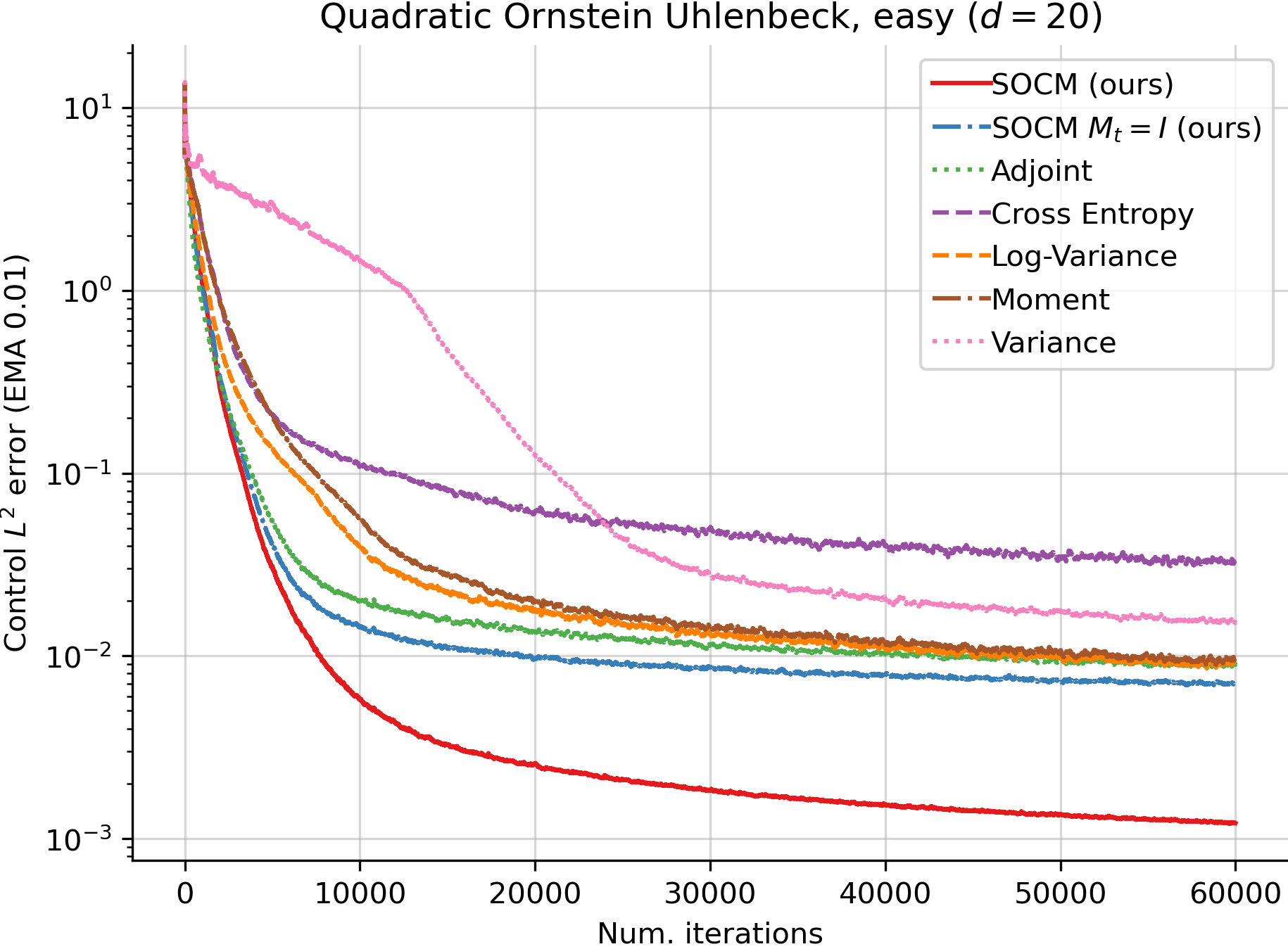
Figure 1: Plots of the $L^{2}$ error incurred by the learned control (left), and the norm squared of the gradient with respect to the parameters $\theta$ of the control (right), for the Quadratic Ornstein Uhlenbeck (easy) setting and for each IDO loss. Both plots show exponential moving averages computed from the trajectories used during training.

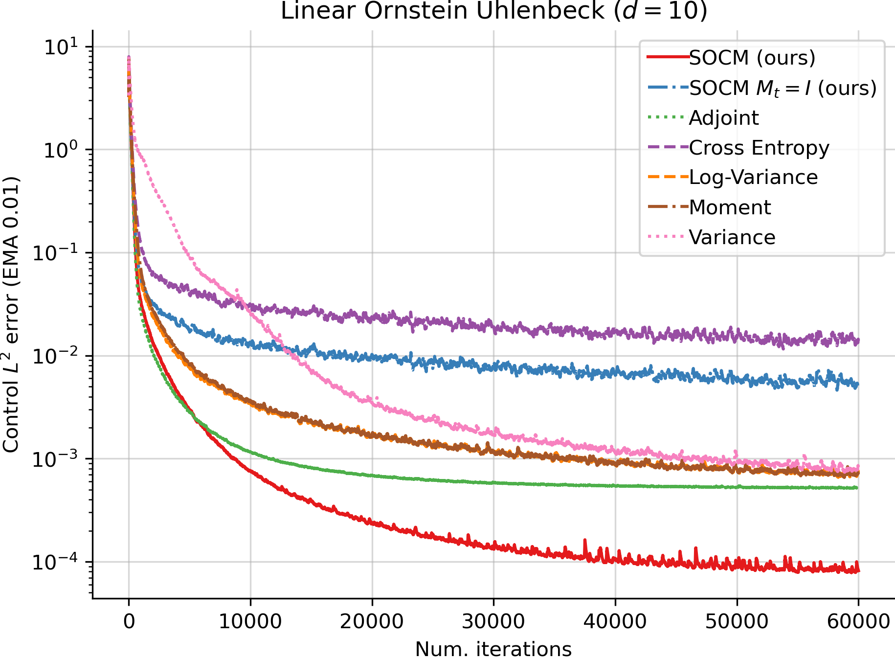
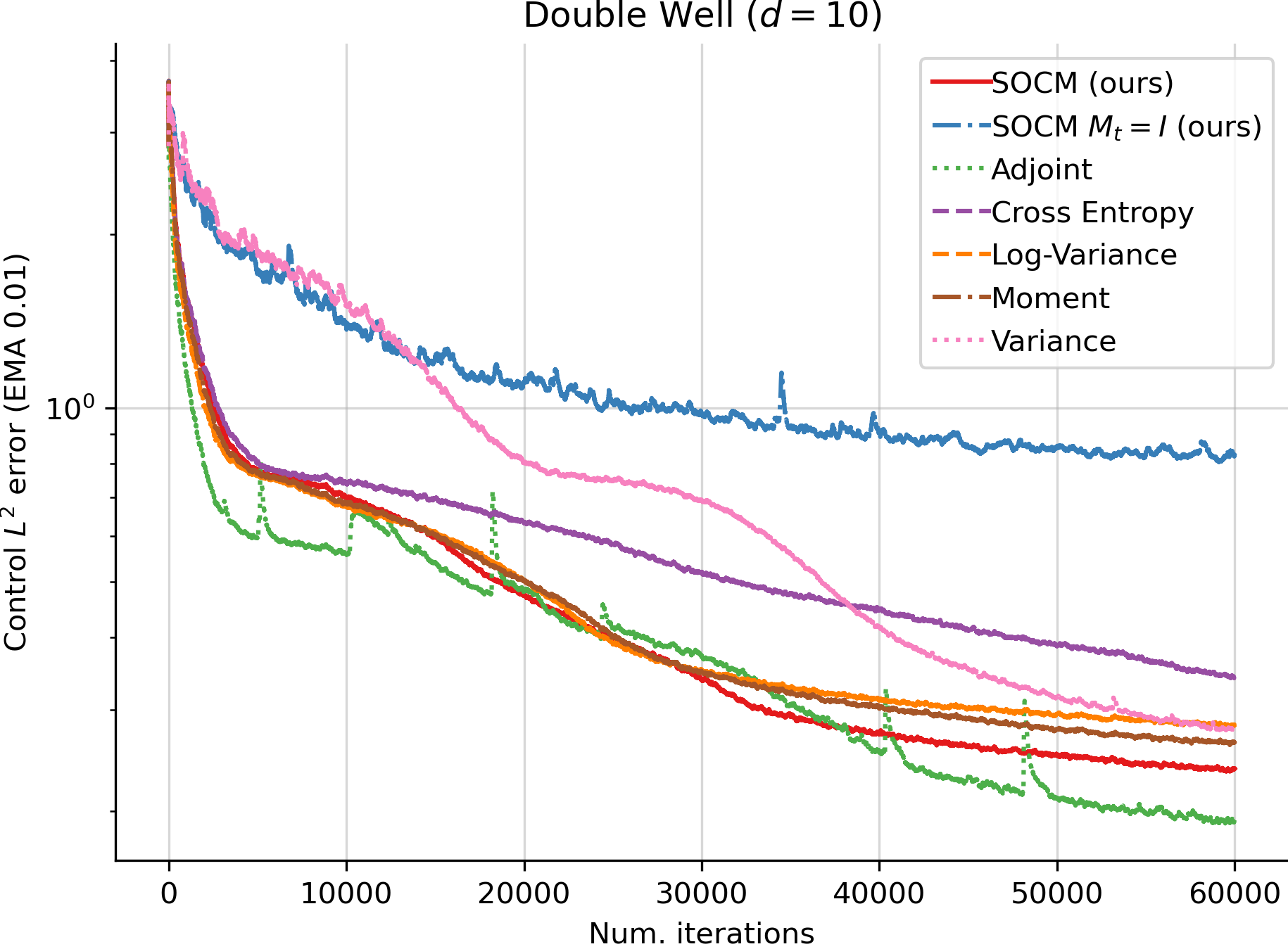
Figure 2: Plots of the $L^{2}$ error incurred by the learned control for the Linear Ornstein Uhlenbeck and Double Well settings.

Figure 3: Plots of the $L^{2}$ error incurred by the learned control (left), and the norm squared of the gradient with respect to the parameters $\theta$ of the control (right), for the Quadratic Ornstein Uhlenbeck (hard) setting and for each IDO loss. All the algorithms use a warm-started control (see App. D).

In Figure 1 (left) we plot the control $L^{2}$ error for each IDO algorithm described in Subsec. 2.2, and for the SOCM algorithm (Algorithm 2), for the Quadratic OU (easy) setting. We also include a version of SOCM where the reparameterization matrices $M_{t}$ are set fixed to the identity $I$, to underline the importance of learning $M_{t}$ properly. We observe that at the end of training, SOCM obtains the lowest $L^{2}$ error, improving over all existing methods by a factor of around ten. The best non-SOCM method is the adjoint method (the relative entropy loss). In Figure 1 (left) we show the squared norm of the gradient of each loss with respect to the parameters $\theta$ of the control. We observe that algorithms with small gradients, i.e., small noise variance, have low error values. For reference, Table 1 shows the average times per iteration for each algorithm.

SOCM	SOCM $M_{t}=I$	Adjoint	Cross entropy	Log-variance	Moment	Variance
0.222	0.090	0.169	0.086	0.117	0.087	0.086

Table 1: Time per iteration for various algorithms in seconds per iteration, for Figure 1.

In Figure 2, we plot the control $L^{2}$ error for Linear Ornstein Uhlenbeck and Double Well. For Linear OU, the error is around five times smaller for SOCM than for any existing method. For Double Well, the SOCM algorithm achieves the second smallest error, slightly behind the adjoint method, but the latter shows instabilities. As we show in Figure 6 in App. E, these instabilities are inherent to the adjoint method and they do not disappear for small learning rates. Both in Figure 1 and Figure 6, we observe that learning the reparameterization matrices is critical to obtain gradient estimates with high signal-to-noise ratio, and consequently a low error.

The costs $f$ and $g$ and the base drift $b$ for Quadratic OU (hard) are five times those of Quadratic OU (easy). Consequently, the factor $\alpha(v,X^{v},B)$ has a much larger variance, and initializing the control neural network without a warm-start yields poor results for the SOCM and cross-entropy losses (see Figure 7 in App. E). Yet, when we use the control warm-start strategy detailed in App. D, Figure 3 shows that SOCM is once again the algorithm that achieves the lowest error and the smallest gradients. Remark that the warm-start control is a reasonable approximation of the optimal control, as the initial control $L^{2}$ error is much lower than in the other figures.

5 Conclusion

Our work introduces Stochastic Optimal Control Matching, a novel Iterative Diffusion Optimization technique for stochastic optimal control that stems from the same philosophy as the conditional score matching loss for diffusion models. That is, the control is learned via a least-squares problem by trying to fit a matching vector field. The training loss is optimized with respect to both the control function and a family of reparameterization matrices which appear in the matching vector field. The optimization with respect to the reparameterization matrices aims at minimizing the variance of the matching vector field. Experimentally, our algorithm achieves lower error than all the existing IDO techniques for stochastic optimal control for four different control settings.

One of the key ideas for deriving the SOCM algorithm is the path-wise reparameterization trick, a novel technique to obtain low-variance estimates of the gradient of the conditional expectation of a functional of a random process with respect to its initial value. An interesting future direction is to use the path-wise reparameterization trick to decrease the variance of the matching vector field for diffusion models.

The main roadblock when we try to apply SOCM to more challenging problems is that the variance of the factor $\alpha(v,X^{v},B)$ explodes when $f$ and/or $g$ are large, or when the dimension $d$ is high. We observe this in Figure 7 in App. E, which is for the Quadratic Ornstein Uhlenbeck (hard) setting but does not use warm-start. The control $L^{2}$ error for the SOCM and cross-entropy losses remains high and fluctuates heavily due to the large variance of $\alpha$. The large variance of $\alpha$ is due to the mismatch between the probability measures induced by the learned control and the optimal control. Similar problems are encountered in out-of-distribution generalization for reinforcement learning, and some approaches may be carried over from that area [Munos et al., 2016].

Appendix A Technical assumptions

Throughout our work, we make the same assumptions as Nüsken and Richter [2021], which are needed for all the objects considered to be well-defined. Namely, we assume that:

1. The set $\mathcal{U}$ of admissible controls is given by

   $$\textstyle U=\{u\in C^{1}(\mathbb{R}^{d}\times[0,T];\mathbb{R}^{d})\,|\,\exists C>0,\,\forall(x,s)\in\mathbb{R}^{d}\times[0,T],\,b(x,s)\leq C(1+|x|)\}.$$ (40)

2. The coefficients $b$ and $\sigma$ are continuously differentiable, $\sigma$ has bounded first-order spatial derivatives, and $(\sigma\sigma^{\top})(x,s)$ is positive definite for all $(x,s)\in\mathbb{R}^{d}\texttimes[0,T]$. Furthermore, there exist constants $C,c_{1},c_{2}>0$ such that

   $$\textstyle\begin{split}\textstyle\|b(x,s)\|\leq C(1+\|x\|),\qquad&\textstyle\text{(linear growth)}\\ \textstyle c_{1}\|\xi\|^{2}\leq\xi^{\top}(\sigma\sigma^{\top})(x,s)\xi\leq c_{2}\|\xi\|^{2},\qquad&\textstyle\text{(ellipticity)}\end{split}$$ (41)

   for all $(x,s)\in\mathbb{R}^{d}\times[0,T]$ and $\xi\in\mathbb{R}^{d}$.

Appendix B Proofs of Sec. 2

Proof of (5)

By Itô’s lemma, we have that

$$\textstyle\begin{split}\textstyle V(X^{u}_{T},T)-V(X^{u}_{t},t)&\textstyle=\int_{t}^{T}\big{(}\partial_{s}V(X^{u}_{s},s)+\langle b(X^{u}_{s},s)+\sigma(X^{u}_{s},s)u(X^{u}_{s},s),\nabla V(X^{u}_{s},s)\rangle\\ \textstyle&\textstyle\qquad+\frac{\lambda}{2}\sum_{i,j=1}^{d}(\sigma\sigma^{\top})_{ij}(X^{u}_{s},s)\partial_{x_{i}}\partial_{x_{j}}V(X^{u}_{s},s)\big{)}\,\mathrm{d}s+S^{u}_{t},\end{split}$$ (42)

where $S^{u}_{t}=\sqrt{\lambda}\int_{t}^{T}\nabla V(X^{u}_{s},s)^{\top}\sigma(X^{u}_{s},s)\,\mathrm{d}B_{s}$. Note that by (LABEL:eq:HJB_setup),

$$\textstyle\partial_{s}V(X^{u}_{s},s)+\langle b(X^{u}_{s},s)+\sigma(X^{u}_{s},s)u(X^{u}_{s},s),\nabla V(X^{u}_{s},s)\rangle$$ (43)

$$\textstyle\qquad+\frac{\lambda}{2}\sum_{i,j=1}^{d}(\sigma\sigma^{\top})_{ij}(X^{u}_{s},s)\partial_{x_{i}}\partial_{x_{j}}V(X^{u}_{s},s)$$ (44)

$$\textstyle=\frac{1}{2}\|(\sigma^{\top}\nabla V)(X^{u}_{s},s)\|^{2}-f(X^{u}_{s},s)+\langle\sigma(X^{u}_{s},s)u(X^{u}_{s},s),\nabla V(X^{u}_{s},s)\rangle$$ (45)

$$\textstyle=\frac{1}{2}\|(\sigma^{\top}\nabla V)(X^{u}_{s},s)+u(X^{u}_{s},s)\|^{2}-\frac{1}{2}\|u(X^{u}_{s},s)\|^{2}-f(X^{u}_{s},s),$$ (46)

and this implies that

$$\textstyle g(X^{u}_{T})-V(X^{u}_{t},t)=\int_{t}^{T}\big{(}\frac{1}{2}\|(\sigma^{\top}\nabla V)(X^{u}_{s},s)+u(X^{u}_{s},s)\|^{2}-\frac{1}{2}\|u(X^{u}_{s},s)\|^{2}-f(X^{u}_{s},s)\big{)}\,\mathrm{d}s+S^{u}_{t}$$ (47)

Since $\mathbb{E}[S^{u}_{t}\,|\,X^{u}_{t}=x]=0$, rearranging (47) and taking the conditional expectation with respect to $X^{u}_{t}$ yields the final result.

Proof of (6)-(7)

By Itô’s lemma, we have that

$$\textstyle\begin{split}\textstyle dV(X_{s},s)&\textstyle=\big{(}\partial_{s}V(X_{s},s)+\langle b(X_{s},s),\nabla V(X_{s},s)\rangle\\ \textstyle&\textstyle\qquad+\frac{\lambda}{2}\sum_{i,j=1}^{d}(\sigma\sigma^{\top})_{ij}(X_{s},s)\partial_{x_{i}}\partial_{x_{j}}V(X_{s},s)\big{)}\,\mathrm{d}s+\sqrt{\lambda}\nabla V(X^{u}_{s},s)^{\top}\sigma(X^{u}_{s},s)\,\mathrm{d}B_{s},\end{split}$$ (48)

Note that by (LABEL:eq:HJB_setup),

$$\textstyle\begin{split}\textstyle&\textstyle\partial_{s}V(X_{s},s)+\langle b(X_{s},s),\nabla V(X_{s},s)\rangle+\frac{\lambda}{2}\sum_{i,j=1}^{d}(\sigma\sigma^{\top})_{ij}(X_{s},s)\partial_{x_{i}}\partial_{x_{j}}V(X_{s},s)\\ \textstyle&\textstyle=\frac{1}{2}\|(\sigma^{\top}\nabla V)(X_{s},s)\|^{2}-f(X_{s},s).\end{split}$$ (49)

Plugging this into (48) concludes the proof.

Proof of (8)

Since $Y_{s}=V(X_{s},s)$ and $Z_{s}=\sigma^{\top}(s)\nabla V(X_{s},s)=-u^{*}(X_{s},s)$ satisfy (7), we have that

$$\textstyle g(X_{T})=Y_{T}=Y_{t}-\int_{t}^{T}(f(X_{s},s)-\frac{1}{2}\|u^{*}(X_{s},s)\|^{2})\,\mathrm{d}s-\sqrt{\lambda}\int_{t}^{T}\langle u^{*}(X_{s},s),\mathrm{d}B_{s}\rangle.$$ (50)

Hence, recalling the definition of the work functional in (10), we have that

$$\textstyle\mathcal{W}(X,t)=Y_{t}+\frac{1}{2}\int_{t}^{T}\|u^{*}(X_{s},s)\|^{2}\,\mathrm{d}s-\sqrt{\lambda}\int_{t}^{T}\langle u^{*}(X_{s},s),\mathrm{d}B_{s}\rangle.$$ (51)

By Novikov’s theorem (Thm. 3), we have that

$$\textstyle\mathbb{E}[\exp(-\lambda^{-1}\mathcal{W}(X,t))|X_{t}]$$ (52)

$$\textstyle=e^{-\lambda^{-1}Y_{t}}\mathbb{E}\big{[}\exp\big{(}\lambda^{-1/2}\int_{t}^{T}\langle u^{*}(X_{s},s),\mathrm{d}B_{s}\rangle-\frac{\lambda^{-1}}{2}\int_{t}^{T}\|u^{*}(X_{s},s)\|^{2}\,\mathrm{d}s\big{)}\big{|}X_{t}\big{]}=e^{-\lambda^{-1}Y_{t}},$$ (53)

which concludes the proof of (8).

Theorem 3 (Novikov’s theorem for deterministic processes).

Let ${\theta_{s}}$ be a locally-$\mathcal{H}_{2}$ process which is adapted to the natural filtration of the Brownian motion $(B_{t})_{t\geq 0}$. Define

$$\textstyle Z(t)=\exp\big{(}\int_{0}^{t}\theta_{s}\,\mathrm{d}B_{s}-\frac{1}{2}\int_{0}^{t}\|\theta_{s}\|^{2}\,\mathrm{d}s\big{)}.$$ (54)

If for each $t\geq 0$,

$$\textstyle\mathbb{E}\big{[}\exp\big{(}\int_{0}^{t}\|\theta_{s}\|^{2}\,\mathrm{d}s\big{)}\big{]}<+\infty,$$ (55)

then for each $t\geq 0$,

$$\textstyle\mathbb{E}[Z(t)]=1.$$ (56)

Moreover, the process $Z(t)$ is a positive martingale, i.e. if ${(\mathcal{F}_{t})}_{t\geq 0}$ is the filtration associated to the Brownian motion ${(B_{t})}_{t\geq 0}$, then for $t\geq s$, $\mathbb{E}[Z_{t}|\mathcal{F}_{s}]=Z_{s}$.

Theorem 4 (Girsanov theorem for deterministic processes).

Let $W={(W_{t})}_{t\in[0,T]}$ be a standard Wiener process, and let $\mathbb{P}$ be its induced probability measure over $C([0,T];\mathbb{R}^{d})$, known as the Wiener measure. Let $Z(t)$ be as defined in (54) and suppose that the assumptions of Theorem 3 hold. Let $(\Omega,\mathcal{F})$ be the $\sigma$-algebra associated to $B_{T}$. For any $F\in\mathcal{F}$, define the measure

$$\textstyle\mathbb{Q}(F)=\mathbb{E}_{\mathbb{P}}[Z(T)\mathbf{1}_{F}]~{}.$$ (57)

$\mathbb{Q}$ is a probability measure because of (56). Under the probability measure $\mathbb{Q}$, the stochastic process $\{W(t)\}_{0\leq t\leq T}$ defined as

$$\textstyle\tilde{W}(t)=W(t)-\int_{0}^{t}\theta_{s}\,\mathrm{d}s$$ (58)

is a standard Wiener process. That is, for any $n\geq 0$ and any $0=t_{0}<t_{1}<\dots<t_{n}$, the increments $\{W(t_{i+1})-W(t_{i})\}_{i=0}^{n-1}$ are independent and $\mathbb{Q}$-Gaussian distributed with mean zero and covariance $(t_{i+1}-t_{i})\mathrm{I}$, which means that for any $\alpha\in\mathbb{R}^{d}$, the moment generating function of $\tilde{W}(t_{i+1})-\tilde{W}(t_{i})$ with respect to $Q$ is as follows:

$$\textstyle\begin{split}\textstyle&\textstyle\mathbb{E}_{Q}[\exp(\langle\alpha,\tilde{W}(t_{i+1})-\tilde{W}(t_{i})\rangle)]\\ \textstyle&\textstyle:=\mathbb{E}_{P}\big{[}\exp\big{(}\big{\langle}\alpha,W(t_{i+1})-\int_{0}^{t_{i+1}}\theta_{s}\,\mathrm{d}s-W(t_{i})+\int_{0}^{t_{i}}\theta_{s}\,\mathrm{d}s\big{\rangle}\big{)}Z(T)\big{]}=\exp\big{(}\frac{(t_{i+1}-t_{i})\|\alpha\|^{2}}{2}\big{)}.\end{split}$$ (59)

Corollary 1 (Girsanov theorem for SDEs).

If the two SDEs

$$\textstyle\mathrm{d}X_{t} \textstyle=b_{1}(X_{t},t)\,\mathrm{d}t+\sigma(X_{t},t)\,\mathrm{d}B_{t},\qquad X_{0}=x_{\mathrm{init}}$$ (60)

$$\textstyle dY_{t} \textstyle=(b_{1}(Y_{t},t)+b_{2}(Y_{t},t))\,\mathrm{d}t+\sigma(Y_{t},t)\,\mathrm{d}B_{t},\qquad Y_{0}=x_{\mathrm{init}}$$ (61)

admit unique strong solutions on $[0,T]$, then for any bounded continuous functional $\Phi$ on $C([0,T])$, we have that

$$\textstyle\mathbb{E}[\Phi(X)] \textstyle=\mathbb{E}\big{[}\Phi(Y)\exp\big{(}-\int_{0}^{T}\sigma(Y_{t},t)^{-1}b_{2}(Y_{t},t)\,\mathrm{d}B_{t}-\frac{1}{2}\int_{0}^{T}\|\sigma(Y_{t},t)^{-1}b_{2}(Y_{t},t)\|^{2}\,\mathrm{d}t\big{)}\big{]}$$ (62)

$$\textstyle=\mathbb{E}\big{[}\Phi(Y)\exp\big{(}-\int_{0}^{T}\sigma(Y_{t},t)^{-1}b_{2}(Y_{t},t)\,d\tilde{B}_{t}+\frac{1}{2}\int_{0}^{T}\|\sigma(Y_{t},t)^{-1}b_{2}(Y_{t},t)\|^{2}\,\mathrm{d}t\big{)}\big{]},$$ (63)

where $\tilde{B}_{t}=B_{t}+\int_{0}^{t}\sigma(Y_{s},s)^{-1}b_{2}(Y_{s},s)\,\mathrm{d}s$.

Lemma 4.

For an arbitrary $v\in\mathcal{U}$, let $\mathbb{P}^{v}$ and $\mathbb{P}$ be respectively the laws of the SDEs

$$\textstyle\mathrm{d}X^{v}_{t} \textstyle=(b(X^{v}_{t},t)+\sigma(t)v(X^{v}_{t},t))\,\mathrm{d}t+\sqrt{\lambda}\sigma(t)\mathrm{d}B_{t},\qquad X^{v}_{0}\sim p_{0},$$ (64)

$$\textstyle\mathrm{d}X_{t} \textstyle=b(X_{t},t)\,\mathrm{d}t+\sqrt{\lambda}\sigma(t)\mathrm{d}B_{t},\qquad X_{0}\sim p_{0}.$$ (65)

We have that

$$\textstyle\frac{d\mathbb{P}}{d\mathbb{P}^{v}}(X^{v}) \textstyle=\exp\big{(}-\lambda^{-1/2}\int_{0}^{T}\langle v(X^{v}_{t},t),\mathrm{d}B^{v}_{t}\rangle+\frac{\lambda^{-1}}{2}\int_{0}^{T}\|v(X^{v}_{t},t)\|^{2}\,\mathrm{d}t\big{)}$$ (66)

$$\textstyle=\exp\big{(}-\lambda^{-1/2}\int_{0}^{T}\langle v(X^{v}_{t},t),\mathrm{d}B_{t}\rangle-\frac{\lambda^{-1}}{2}\int_{0}^{T}\|v(X^{v}_{t},t)\|^{2}\,\mathrm{d}t\big{)},$$ (67)

$$\textstyle\frac{d\mathbb{P}^{v}}{d\mathbb{P}}(X) \textstyle=\exp\big{(}\lambda^{-1/2}\int_{0}^{T}\langle v(X_{t},t),\mathrm{d}B_{t}\rangle-\frac{\lambda^{-1}}{2}\int_{0}^{T}\|v(X_{t},t)\|^{2}\,\mathrm{d}t\big{)}.$$ (68)

where $B^{v}_{t}:=B_{t}-\lambda^{-1/2}\int_{0}^{t}v(X^{v}_{s},s)\,\mathrm{d}s$. For the optimal control $u^{*}$, we have that

$$\textstyle\frac{d\mathbb{P}}{d\mathbb{P}^{u^{*}}}(X^{u^{*}}) \textstyle=\exp\big{(}\lambda^{-1}\big{(}-V(X_{0}^{u^{*}},0)+\mathcal{W}(X^{u^{*}},0)\big{)}\big{)},$$ (69)

$$\textstyle\frac{d\mathbb{P}^{u^{*}}}{d\mathbb{P}}(X) \textstyle=\exp\big{(}\lambda^{-1}\big{(}V(X_{0},0)-\mathcal{W}(X,0)\big{)}\big{)},$$ (70)

where the functional $\mathcal{W}$ is defined in (10).

Proof.

The proof of (66)-(68) follows directly from Cor. 1. To prove (70), we use that by (51),

$$\textstyle\mathcal{W}(X,0)=V(X_{0},0)+\frac{1}{2}\int_{0}^{T}\|u^{*}(X_{s},s)\|^{2}\,\mathrm{d}s-\sqrt{\lambda}\int_{0}^{T}\langle u^{*}(X_{s},s),\mathrm{d}B_{s}\rangle,$$ (71)

which implies that

$$\textstyle\frac{d\mathbb{P}^{u^{*}}}{d\mathbb{P}}(X) \textstyle=\exp\big{(}\lambda^{-1/2}\int_{0}^{T}\langle u^{*}(X_{t},t),\mathrm{d}B_{t}\rangle-\frac{\lambda^{-1}}{2}\int_{0}^{T}\|u^{*}(X_{t},t)\|^{2}\,\mathrm{d}t\big{)}$$ (72)

$$\textstyle=\exp\big{(}\lambda^{-1}\big{(}V(X_{0},0)-\mathcal{W}(X,0)\big{)}\big{)}.$$ (73)

To prove (69), we use that since $\mathrm{d}X^{u^{*}}_{t}=b(X^{u^{*}}_{t},t)\,\mathrm{d}t+\sqrt{\lambda}\sigma(t)\mathrm{d}B_{t}^{u^{*}}$, equation (71) holds if we replace $X$ and $B$ by $X^{u^{*}}$ and $B^{u^{*}}$, which reads

$$\textstyle\mathcal{W}(X^{u^{*}},0)=V(X^{u^{*}}_{0},0)+\frac{1}{2}\int_{t}^{T}\|u^{*}(X^{u^{*}}_{s},s)\|^{2}\,\mathrm{d}s-\sqrt{\lambda}\int_{t}^{T}\langle u^{*}(X^{u^{*}}_{s},s),\mathrm{d}B^{v}_{s}\rangle.$$ (74)

Hence,

$$\textstyle\frac{d\mathbb{P}}{d\mathbb{P}^{u^{*}}}(X^{u^{*}}) \textstyle=\exp\big{(}-\lambda^{-1/2}\int_{0}^{T}\langle u^{*}(X^{u^{*}}_{t},t),\mathrm{d}B^{u^{*}}_{t}\rangle+\frac{\lambda^{-1}}{2}\int_{0}^{T}\|u^{*}(X^{u^{*}}_{t},t)\|^{2}\,\mathrm{d}t\big{)}$$ (75)

$$\textstyle=\exp\big{(}\lambda^{-1}\big{(}-V(X_{0}^{u^{*}},0)+\mathcal{W}(X^{u^{*}},0)\big{)}\big{)}.$$ (76)

∎

Lemma 5.

The following expression holds:

$$\textstyle\mathbb{E}_{\mathbb{P}^{u}}\big{[}\log\frac{d\mathbb{P}^{u}}{d\mathbb{P}^{u^{*}}}\big{]} \textstyle=\lambda^{-1}\mathbb{E}\big{[}\int_{0}^{T}\big{(}\frac{1}{2}\|u(X^{u}_{t},t)\|^{2}+f(X^{u}_{t},t)\big{)}\,\mathrm{d}t+g(X^{u}_{T})-V(X^{u}_{0},0)\big{]},$$ (77)

Proof.

To prove (77), we write

$$\textstyle\log\frac{d\mathbb{P}^{u^{*}}}{d\mathbb{P}^{u}}(X^{u}) \textstyle=\log\big{(}\frac{d\mathbb{P}^{u^{*}}}{d\mathbb{P}}(X^{u})\frac{d\mathbb{P}}{d\mathbb{P}^{u}}(X^{u})\big{)}=\log\frac{d\mathbb{P}^{u^{*}}}{d\mathbb{P}}(X^{u})+\log\frac{d\mathbb{P}}{d\mathbb{P}^{u}}(X^{u})$$ (78)

$$\textstyle=\lambda^{-1}\big{(}V(X_{0}^{u},0)-\int_{0}^{T}f(X^{u}_{t},t)\,\mathrm{d}t-g(X^{u}_{T})\big{)}$$ (79)

$$\textstyle\qquad-\lambda^{-1/2}\int_{0}^{T}\langle u(X^{u}_{t},t),\mathrm{d}B_{t}\rangle-\frac{\lambda^{-1}}{2}\int_{0}^{T}\|u(X^{u}_{t},t)\|^{2}\,\mathrm{d}t~{}.$$ (80)

Since $\mathbb{E}_{\mathbb{P}^{u}}\big{[}\log\frac{d\mathbb{P}^{u}}{d\mathbb{P}^{u^{*}}}\big{]}=-\mathbb{E}_{\mathbb{P}^{u}}\big{[}\log\frac{d\mathbb{P}^{u^{*}}}{d\mathbb{P}^{u}}\big{]}$, and $\mathbb{E}_{\mathbb{P}^{u}}\big{[}\int_{0}^{T}\langle u(X^{u}_{t},t),\mathrm{d}B_{t}\rangle]=0$, the result follows. ∎

Proposition 3.

(i) The following two expressions hold for arbitrary controls $u,v$ in the class $\mathcal{U}$ of admissible controls:

$$\textstyle\tilde{\mathcal{L}}_{\mathrm{CE}}(u)=\mathbb{E}_{\mathbb{P}^{u^{*}}}\big{[}\log\frac{d\mathbb{P}^{u^{*}}}{d\mathbb{P}^{u}}\big{]} \textstyle=\mathbb{E}\big{[}\big{(}-\lambda^{-1/2}\int_{0}^{T}\langle u(X^{v}_{t},t),\mathrm{d}B_{t}\rangle-\lambda^{-1}\int_{0}^{T}\langle u(X^{v}_{t},t),v(X^{v}_{t},t)\rangle\,\mathrm{d}t$$ (81)

$$\textstyle\qquad\qquad\quad+\frac{\lambda^{-1}}{2}\int_{0}^{T}\|u(X^{v}_{t},t)\|^{2}\,\mathrm{d}t+\lambda^{-1}\big{(}V(X_{0}^{v},0)-\mathcal{W}(X^{v},0)\big{)}\big{)}$$ (82)

$$\textstyle\qquad\qquad\times\exp\big{(}\lambda^{-1}\big{(}V(X_{0}^{v},0)-\mathcal{W}(X^{v},0)\big{)}$$ (83)

$$\textstyle\qquad\qquad\qquad\quad-\lambda^{-1/2}\int_{0}^{T}\langle v(X^{v}_{t},t),\mathrm{d}B_{t}\rangle-\frac{\lambda^{-1}}{2}\int_{0}^{T}\|v(X^{v}_{t},t)\|^{2}\,\mathrm{d}t\big{)}\big{]},$$ (84)

$$\textstyle\tilde{\mathcal{L}}_{\mathrm{CE}}(u) \textstyle=\frac{\lambda^{-1}}{2}\mathbb{E}\big{[}\int_{0}^{T}\|u^{*}(X^{u^{*}}_{t},t)-u(X^{u^{*}}_{t},t)\|^{2}\,\mathrm{d}t\big{]}.$$ (85)

When $p_{0}$ is concentrated at a single point $x_{\mathrm{init}}$, the terms $V(x_{\mathrm{init}},0)$ are constant and can be removed without modifying the landscape. In other words, $\tilde{\mathcal{L}}_{\mathrm{CE}}$ and $\mathcal{L}_{\mathrm{CE}}$ are equal up to constant terms and constant factors.

(ii) When $p_{0}$ is a generic probability measure, $\tilde{\mathcal{L}}_{\mathrm{CE}}$ and $\mathcal{L}_{\mathrm{CE}}$ have different landscapes, and $\mathcal{L}_{\mathrm{CE}}(u)=\mathbb{E}_{\mathbb{P}^{u^{*}}}\big{[}\log\frac{d\mathbb{P}^{u^{*}}}{d\mathbb{P}^{u}}\exp\big{(}-\lambda^{-1}V(X^{u^{*}}_{0},0)\big{)}\big{]}$. $u^{*}$ is still the only minimizer of the loss $\mathcal{L}_{\mathrm{CE}}$, and for some constant $K$, we have that

$$\textstyle\mathcal{L}_{\mathrm{CE}}(u,0)=\frac{\lambda^{-1}}{2}\mathbb{E}\big{[}\int_{0}^{T}\|u^{*}(X^{u^{*}}_{t},t)-u(X^{u^{*}}_{t},t)\|^{2}\,\mathrm{d}t\exp\big{(}-\lambda^{-1}V(X^{u^{*}}_{0},0)\big{)}\big{]}+K.$$ (86)

Proof.

We begin with the proof of (i), and prove (81) first. Note that by the Girsanov theorem (Thm. 4),

$$\textstyle\begin{split}\textstyle\mathbb{E}_{\mathbb{P}^{u^{*}}}\big{[}\log\frac{d\mathbb{P}^{u^{*}}}{d\mathbb{P}^{u}}(X^{u^{*}})\big{]}&\textstyle=-\mathbb{E}_{\mathbb{P}^{u^{*}}}\big{[}\log\frac{d\mathbb{P}^{u}}{d\mathbb{P}^{u^{*}}}(X^{u^{*}})\big{]}=-\mathbb{E}_{\mathbb{P}^{u^{*}}}\big{[}\log\frac{d\mathbb{P}^{u}}{d\mathbb{P}}(X^{u^{*}})+\log\frac{d\mathbb{P}}{d\mathbb{P}^{u^{*}}}(X^{u^{*}})\big{]}\\ \textstyle&\textstyle=-\mathbb{E}_{\mathbb{P}^{v}}\big{[}\big{(}\log\frac{d\mathbb{P}^{u}}{d\mathbb{P}}(X^{v})+\log\frac{d\mathbb{P}}{d\mathbb{P}^{u^{*}}}(X^{v})\big{)}\frac{d\mathbb{P}^{u^{*}}}{d\mathbb{P}}(X^{v})\frac{d\mathbb{P}}{d\mathbb{P}^{v}}(X^{v})\big{]}\end{split}$$ (87)

Note that by equations (68) and (70),

$$\textstyle\begin{split}\textstyle\log\frac{d\mathbb{P}^{u}}{d\mathbb{P}}(X^{v})&\textstyle=\lambda^{-1/2}\int_{0}^{T}\langle u(X^{v}_{t},t),\mathrm{d}B^{v}_{t}\rangle-\frac{\lambda^{-1}}{2}\int_{0}^{T}\|u(X^{v}_{t},t)\|^{2}\,\mathrm{d}t,\\ \textstyle&\textstyle=\lambda^{-1/2}\int_{0}^{T}\langle u(X^{v}_{t},t),\mathrm{d}B_{t}\rangle+\lambda^{-1}\int_{0}^{T}\langle u(X^{v}_{t},t),v(X^{v}_{t},t)\rangle\,\mathrm{d}t-\frac{\lambda^{-1}}{2}\int_{0}^{T}\|u(X^{v}_{t},t)\|^{2}\,\mathrm{d}t,\\ \textstyle\log\frac{d\mathbb{P}}{d\mathbb{P}^{u^{*}}}(X^{v})&\textstyle=\lambda^{-1}\big{(}-V(X_{0}^{v},0)+\mathcal{W}(X^{v},0)\big{)}.\end{split}$$ (88)

where $B^{v}_{t}:=B_{t}+\lambda^{-1/2}\int_{0}^{t}v(X^{v}_{s},s)\,\mathrm{d}s$. Also,

$$\textstyle\begin{split}\textstyle\frac{d\mathbb{P}^{u^{*}}}{d\mathbb{P}}(X^{v})&\textstyle=\exp\big{(}\lambda^{-1}\big{(}V(X_{0}^{v},0)-\mathcal{W}(X^{v},0)\big{)}\big{)},\\ \textstyle\frac{d\mathbb{P}}{d\mathbb{P}^{v}}(X^{v})&\textstyle=\exp\big{(}-\lambda^{-1/2}\int_{0}^{T}\langle v(X^{v}_{t},t),\mathrm{d}B_{t}\rangle-\frac{\lambda^{-1}}{2}\int_{0}^{T}\|v(X^{v}_{t},t)\|^{2}\,\mathrm{d}t\big{)}.\end{split}$$ (89)

If we plug (88) and (89) into the right-hand side of (87), we obtain

$$\textstyle\begin{split}\textstyle&\textstyle\mathbb{E}_{\mathbb{P}^{u^{*}}}\big{[}\log\frac{d\mathbb{P}^{u^{*}}}{d\mathbb{P}^{u}}(X^{u^{*}})\big{]}=-\mathbb{E}_{\mathbb{P}^{u^{*}}}\big{[}(\log\frac{d\mathbb{P}^{u}}{d\mathbb{P}}(X^{v})+\log\frac{d\mathbb{P}}{d\mathbb{P}^{u^{*}}}(X^{v}))\frac{d\mathbb{P}^{u^{*}}}{d\mathbb{P}}(X^{v})\frac{d\mathbb{P}}{d\mathbb{P}^{u}}(X^{v})\big{]}\\ \textstyle&\textstyle=-\mathbb{E}\big{[}\big{(}\lambda^{-1/2}\int_{0}^{T}\langle u(X^{v}_{t},t),\mathrm{d}B_{t}\rangle+\lambda^{-1}\int_{0}^{T}\langle u(X^{v}_{t},t),v(X^{v}_{t},t)\rangle\,\mathrm{d}t\\ \textstyle&\textstyle\qquad\qquad\quad-\frac{\lambda^{-1}}{2}\int_{0}^{T}\|u(X^{v}_{t},t)\|^{2}\,\mathrm{d}t+\lambda^{-1}\big{(}-V(X_{0}^{v},0)+\mathcal{W}(X^{v},0)\big{)}\big{)}\\ \textstyle&\textstyle\qquad\quad\times\exp\big{(}\lambda^{-1}\big{(}V(X_{0}^{v},0)-\mathcal{W}(X^{v},0)\big{)}-\lambda^{-1/2}\int_{0}^{T}\langle v(X^{v}_{t},t),\mathrm{d}B_{t}\rangle-\frac{\lambda^{-1}}{2}\int_{0}^{T}\|v(X^{v}_{t},t)\|^{2}\,\mathrm{d}t\big{)}\big{]},\end{split}$$ (90)

which concludes the proof.

To show (85), we use that by Cor. 1,

$$\textstyle\frac{d\mathbb{P}^{u}}{d\mathbb{P}^{u^{*}}}(X^{u^{*}})\!=\!\exp\big{(}\!-\!\lambda^{-1/2}\int_{0}^{T}\langle u^{*}(X^{u^{*}}_{t},t)\!-\!u(X^{u^{*}}_{t},t),\mathrm{d}B_{t}\rangle\!-\!\frac{\lambda^{-1}}{2}\int_{0}^{T}\|u^{*}(X^{u^{*}}_{t},t)\!-\!u(X^{u^{*}}_{t},t)\|^{2}\,\mathrm{d}t\big{)}.$$ (91)

Hence,

$$\textstyle\mathbb{E}_{\mathbb{P}^{u^{*}}}\big{[}\log\frac{d\mathbb{P}^{u^{*}}}{d\mathbb{P}^{u}}\big{]}=-\mathbb{E}_{\mathbb{P}^{u^{*}}}\big{[}\log\frac{d\mathbb{P}^{u}}{d\mathbb{P}^{u^{*}}}\big{]}=\frac{\lambda^{-1}}{2}\mathbb{E}\big{[}\int_{0}^{T}\|u^{*}(X^{u^{*}}_{t},t)-u(X^{u^{*}}_{t},t)\|^{2}\,\mathrm{d}t\big{]}.$$ (92)

Next, we prove (ii). The first instance of $V(X_{0}^{v},0)$ in (81) can be removed without modifying the landscape of the loss. Hence, we are left with

$$\textstyle\bar{\mathcal{L}}_{\mathrm{CE}}(u) \textstyle=\mathbb{E}\big{[}\big{(}-\lambda^{-1/2}\int_{0}^{T}\langle u(X^{v}_{t},t),\mathrm{d}B^{v}_{t}\rangle-\lambda^{-1}\int_{0}^{T}\langle u(X^{v}_{t},t),v(X^{v}_{t},t)\rangle\,\mathrm{d}t$$ (93)

$$\textstyle\qquad\qquad\quad+\frac{\lambda^{-1}}{2}\int_{0}^{T}\|u(X^{v}_{t},t)\|^{2}\,\mathrm{d}t-\lambda^{-1}\mathcal{W}(X^{v},0)\big{)}$$ (94)

$$\textstyle\qquad\times\exp\big{(}\lambda^{-1}\big{(}V(X_{0}^{v},0)\!-\!\mathcal{W}(X^{v},0)\big{)}\!-\!\lambda^{-1/2}\int_{0}^{T}\langle v(X^{v}_{t},t),\mathrm{d}B_{t}\rangle\!-\!\frac{\lambda^{-1}}{2}\int_{0}^{T}\|v(X^{v}_{t},t)\|^{2}\,\mathrm{d}t\big{)}\big{]}$$ (95)

And this can be expressed as

$$\textstyle\bar{\mathcal{L}}_{\mathrm{CE}}(u) \textstyle=\mathbb{E}\big{[}g(u;X_{0}^{v})\exp\big{(}\lambda^{-1}V(X_{0}^{v},0)\big{)}\big{]},$$ (96)

where

$$\textstyle g(u;x) \textstyle=\mathbb{E}\big{[}\big{(}-\lambda^{-1/2}\int_{0}^{T}\langle u(X^{v}_{t},t),\mathrm{d}B^{v}_{t}\rangle-\lambda^{-1}\int_{0}^{T}\langle u(X^{v}_{t},t),v(X^{v}_{t},t)\rangle\,\mathrm{d}t$$ (97)

$$\textstyle\qquad\qquad\quad+\frac{\lambda^{-1}}{2}\int_{0}^{T}\|u(X^{v}_{t},t)\|^{2}\,\mathrm{d}t-\lambda^{-1}\mathcal{W}(X^{v},0)\big{)}$$ (98)

$$\textstyle\qquad\times\exp\big{(}-\lambda^{-1}\mathcal{W}(X^{v},0)\!-\!\lambda^{-1/2}\int_{0}^{T}\langle v(X^{v}_{t},t),\mathrm{d}B_{t}\rangle\!-\!\frac{\lambda^{-1}}{2}\int_{0}^{T}\|v(X^{v}_{t},t)\|^{2}\,\mathrm{d}t\big{)}|X_{0}^{v}=x\big{]}.$$ (99)

If we consider $g(u;x)$ as a loss function for $u$, note that it is equivalent to the loss $\bar{L}_{\mathrm{CE}}(u)$ equation in (93) for the choice $p_{0}=\delta_{x}$, i.e., $p_{0}$ concentrated at $x$. Since the optimal control $u^{*}$ is independent of the starting distribution $p_{0}$, we deduce that $u^{*}$ is the unique minimizer of $g(u;x)$, for all $x\in\mathbb{R}^{d}$. In consequence, $u^{*}$ is the unique minimizer of $\mathcal{L}_{\mathrm{CE}}(u)=\mathbb{E}[g(u;X_{0}^{v})]$.

To prove (86), note that up to a constant term, the only difference between $\bar{\mathcal{L}}_{\mathrm{CE}}(u)$ and $\mathcal{L}_{\mathrm{CE}}(u)$ is the expectation is reweighted importance weight $\exp\big{(}-\lambda^{-1}V(X_{0}^{v},0)\big{)}$. ∎

Lemma 6.

(i) We can rewrite

$$\tilde{\mathcal{L}}_{\mathrm{Var}_{v}}(u) =\mathrm{Var}\big{(}\exp\big{(}\tilde{Y}^{u,v}_{T}-\lambda^{-1}g(X^{v}_{T})+\lambda^{-1}V(X^{v}_{0},0)\big{)}\big{)},$$ (100)

$$\tilde{\mathcal{L}}^{\mathrm{log}}_{\mathrm{Var}_{v}}(u) =\mathrm{Var}\big{(}\tilde{Y}^{u,v}_{T}-\lambda^{-1}g(X^{v}_{T})+\lambda^{-1}V(X^{v}_{0},0)\big{)}.$$ (101)

When $p_{0}$ is concentrated at $x_{\mathrm{init}}$, the terms $V(x_{\mathrm{init}},0)$ are constants and can be removed without modifying the landscape. In other words, $\tilde{\mathcal{L}}_{\mathrm{Var}_{v}}$ and $\tilde{\mathcal{L}}_{\mathrm{Var}_{v}}^{\mathrm{log}}$ are equal to $\mathcal{L}_{\mathrm{Var}_{v}}$ and $\mathcal{L}_{\mathrm{Var}_{v}}^{\mathrm{log}}$ up to a constant term and a constant factor, respectively.

(ii) When $p_{0}$ is general, $\tilde{\mathcal{L}}_{\mathrm{Var}_{v}}$ and $\mathcal{L}_{\mathrm{Var}_{v}}$ have a different landscape, and the optimum of $\mathcal{L}_{\mathrm{Var}_{v}}$ may be different from $u^{*}$. A related loss that does preserve the optimum is:

$$\textstyle\bar{\mathcal{L}}_{\mathrm{Var}_{v}}(u) \textstyle=\mathbb{E}[\mathrm{Var}_{\mathbb{P}^{v}}(\frac{d\mathbb{P}^{u^{*}}}{d\mathbb{P}^{u}}(X^{v})|X^{v}_{0})\exp(-\lambda^{-1}V(X^{v}_{0},0))]$$ (102)

$$\textstyle=\mathbb{E}[\mathrm{Var}\big{(}\exp(\tilde{Y}^{u,v}_{T}-\lambda^{-1}g(X^{v}_{T}))|X^{v}_{0}\big{)}].$$ (103)

In practice, this is implemented by sampling the $m$ trajectories in one batch starting at the same point $X^{v}_{0}$.

(iii) Also, $\tilde{\mathcal{L}}_{\mathrm{Var}_{v}}^{\mathrm{log}}$ and $\mathcal{L}_{\mathrm{Var}_{v}}^{\mathrm{log}}$ have a different landscape, and the optimum of $\mathcal{L}_{\mathrm{Var}_{v}}^{\mathrm{log}}$ may be different from $u^{*}$. In particular, $\mathcal{L}_{\mathrm{Var}_{v}}^{\mathrm{log}}(u)=\mathrm{Var}_{\mathbb{P}^{v}}(\log\frac{d\mathbb{P}^{u^{*}}}{d\mathbb{P}^{u}}(X^{v})\exp(-\lambda^{-1}V(X^{v}_{0},0)))$. A loss that does preserve the optimum $u^{*}$ is

$$\textstyle\bar{\mathcal{L}}_{\mathrm{Var}_{v}}^{\mathrm{log}}(u) \textstyle=\mathbb{E}[\mathrm{Var}_{\mathbb{P}^{v}}(\log\frac{d\mathbb{P}^{u^{*}}}{d\mathbb{P}^{u}}(X^{v})|X^{v}_{0})\exp(-\lambda^{-1}V(X^{v}_{0},0))]$$ (104)

$$\textstyle=\mathbb{E}[\mathrm{Var}\big{(}\tilde{Y}^{u,v}_{T}-\lambda^{-1}g(X^{v}_{T})|X^{v}_{0}\big{)}].$$ (105)

Proof.

Using (70) and (66), we have that

$$\textstyle\frac{d\mathbb{P}^{u^{*}}}{d\mathbb{P}}(X^{v}) \textstyle=\exp\big{(}\lambda^{-1}\big{(}V(X^{v}_{0},0)-\mathcal{W}(X^{v},0)\big{)}\big{)},$$ (106)

$$\textstyle\frac{d\mathbb{P}}{d\mathbb{P}^{u}}(X^{v}) \textstyle=\exp\big{(}-\lambda^{-1/2}\int_{0}^{T}\langle u(X^{v}_{t},t),\mathrm{d}B^{v}_{t}\rangle+\frac{\lambda^{-1}}{2}\int_{0}^{T}\|u(X^{v}_{t},t)\|^{2}\,\mathrm{d}t\big{)}$$ (107)

$$\textstyle=\exp\big{(}-\lambda^{-1/2}\int_{0}^{T}\langle u(X^{v}_{t},t),\mathrm{d}B_{t}\rangle-\lambda^{-1}\int_{0}^{T}\langle u(X^{v}_{t},t),v(X^{v}_{t},t)\rangle\,\mathrm{d}t$$ (108)

$$\textstyle\qquad\qquad+\frac{\lambda^{-1}}{2}\int_{0}^{T}\|u(X^{v}_{t},t)\|^{2}\,\mathrm{d}t\big{)}.$$ (109)

Hence,

$$\textstyle\log\frac{d\mathbb{P}^{u^{*}}}{d\mathbb{P}^{u}}(X^{v})=\log\frac{d\mathbb{P}^{u^{*}}}{d\mathbb{P}}(X^{v})+\log\frac{d\mathbb{P}}{d\mathbb{P}^{u}}(X^{v})=\tilde{Y}^{u,v}_{T}-\lambda^{-1}g(X^{v}_{T})+\lambda^{-1}V(X^{v}_{0},0).$$ (110)

Since $\tilde{\mathcal{L}}_{\mathrm{Var}_{v}}(u)=\mathrm{Var}_{\mathbb{P}^{v}}(\frac{d\mathbb{P}^{u^{*}}}{d\mathbb{P}^{u}})$ and $\tilde{\mathcal{L}}_{\mathrm{Var}_{v}}^{\mathrm{log}}(u)=\mathrm{Var}_{\mathbb{P}^{v}}(\log\frac{d\mathbb{P}^{u^{*}}}{d\mathbb{P}^{u}})$, this concludes the proof of (i).

To prove (ii), note that for general $p_{0}$, $V(X^{v}_{0},0)$ is no longer a constant, but it is if we condition on $X^{v}_{0}$. The proof of (iii) is analogous. ∎

Appendix C Proofs of Sec. 3

C.1 Proof of Thm. 1 and Prop. 2

We prove Thm. 1 and Prop. 2 at the same time. Recall that by (9), the optimal control is of the form $u^{*}(x,t)=-\sigma(t)^{\top}\nabla V(x,t)$. Consider the loss

$$\textstyle\tilde{\mathcal{L}}(u)=\mathbb{E}\big{[}\frac{1}{T}\int_{0}^{T}\big{\|}u(X_{t},t)+\sigma(t)^{\top}\nabla V(X_{t},t)\big{\|}^{2}\,\mathrm{d}t\,\exp\big{(}-\lambda^{-1}\int_{0}^{T}f(X_{t},t)\,\mathrm{d}t-\lambda^{-1}g(X_{T})\big{)}\big{]}.$$ (111)

Clearly, the unique optimum of $\tilde{\mathcal{L}}$ is $-\sigma(t)^{\top}\nabla V$. We can rewrite $\tilde{\mathcal{L}}$ as

$$\textstyle\tilde{\mathcal{L}}(u) \textstyle=\mathbb{E}\big{[}\frac{1}{T}\int_{0}^{T}\big{(}\big{\|}u(X_{t},t)\big{\|}^{2}+2\langle u(X_{t},t),\sigma(t)^{\top}\nabla V(X_{t},t)\rangle+\|\sigma(t)^{\top}\nabla V(X_{t},t)\big{\|}^{2}\big{)}\,\mathrm{d}t$$ (112)

$$\textstyle\qquad\qquad\times\exp\big{(}-\lambda^{-1}\int_{0}^{T}f(X_{t},t)\,\mathrm{d}t-\lambda^{-1}g(X_{T})\big{)}\big{]}~{}.$$ (113)

Hence, we can express $\tilde{\mathcal{L}}$ as a sum of three terms: one involving $\|u(X_{t},t)\|^{2}$, another involving $\langle u(X_{t},t),\sigma(t)^{\top}V(X_{t},t)\rangle$, and a third one, which is constant with respect to $u$, involving $\|\nabla V(X_{t},t)\|^{2}$. The following lemma provides an alternative expression for the cross term:

Lemma 7.

The following equality holds:

$$\textstyle\begin{split}\textstyle&\textstyle\mathbb{E}\big{[}\frac{1}{T}\int_{0}^{T}\langle u(X_{t},t),\sigma(t)^{\top}\nabla V(X_{t},t)\rangle\,\mathrm{d}t\,\exp\big{(}-\lambda^{-1}\int_{0}^{T}f(X_{t},t)\,\mathrm{d}t-\lambda^{-1}g(X_{T})\big{)}\big{]}\\ \textstyle&\textstyle=-\lambda\mathbb{E}\big{[}\frac{1}{T}\int_{0}^{T}\big{\langle}u(X_{t},t),\sigma(t)^{\top}\nabla_{x}\mathbb{E}\big{[}\exp\big{(}-\lambda^{-1}\int_{t}^{T}f(X_{s},s)\,\mathrm{d}s-\lambda^{-1}g(X_{T})\big{)}\big{|}X_{t}=x\big{]}\big{\rangle}\,\mathrm{d}t\\ \textstyle&\textstyle\qquad\qquad\times\exp\big{(}-\lambda^{-1}\int_{0}^{t}f(X_{s},s)\,\mathrm{d}s\big{)}\big{]}.\end{split}$$ (114)

Proof.

Recall the definition of $\mathcal{W}(X,t)$ in (71), which means that

$$\textstyle\mathcal{W}(X,0)=\mathcal{W}(X,t)+\int_{0}^{t}f(X_{s},s)\,\mathrm{d}s.$$ (115)

Let $\{\mathcal{F}_{t}\}_{t\in[0,T]}$ be the filtration generated by the Brownian motion $B$. Then, equation (9) implies that

$$\textstyle\sigma(t)^{\top}\nabla V(X_{t},t)=-\frac{\lambda\sigma(t)^{\top}\nabla_{x}\mathbb{E}\big{[}\exp\big{(}-\lambda^{-1}\mathcal{W}(X,t)\big{)}\big{|}\mathcal{F}_{t}\big{]}}{\mathbb{E}\big{[}\exp\big{(}-\lambda^{-1}\mathcal{W}(X,t)\big{)}\big{|}\mathcal{F}_{t}\big{]}}$$ (116)

We proceed as follows:

$$\textstyle\begin{split}\textstyle&\textstyle\mathbb{E}\big{[}\frac{1}{T}\int_{0}^{T}\langle u(X_{t},t),\sigma(t)^{\top}\nabla V(X_{t},t)\rangle\,\mathrm{d}t\,\exp\big{(}-\lambda^{-1}\mathcal{W}(X,0)\big{)}\big{]}\\ \textstyle&\textstyle\stackrel{{\scriptstyle\text{(i)}}}{{=}}-\lambda\mathbb{E}\big{[}\frac{1}{T}\int_{0}^{T}\big{\langle}u(X_{t},t),\frac{\sigma(t)^{\top}\nabla_{x}\mathbb{E}\big{[}\exp\big{(}-\lambda^{-1}\mathcal{W}(X,t)\big{)}\big{|}\mathcal{F}_{t}\big{]}}{\mathbb{E}\big{[}\exp\big{(}-\lambda^{-1}\mathcal{W}(X,t)\big{)}\big{|}\mathcal{F}_{t}\big{]}}\big{\rangle}\,\mathrm{d}t\\ \textstyle&\textstyle\qquad\qquad\qquad\times\mathbb{E}\big{[}\exp\big{(}-\lambda^{-1}\mathcal{W}(X,t)\big{)}\big{|}\mathcal{F}_{t}\big{]}\exp\big{(}-\lambda^{-1}\int_{0}^{t}f(X_{t},t)\,\mathrm{d}t\big{)}\big{]}\\ \textstyle&\textstyle=-\lambda\mathbb{E}\big{[}\frac{1}{T}\int_{0}^{T}\big{\langle}u(X_{t},t),\nabla_{x}\mathbb{E}\big{[}\exp\big{(}-\lambda^{-1}\mathcal{W}(X,t)\big{)}\big{|}\mathcal{F}_{t}\big{]}\big{\rangle}\,\mathrm{d}t\exp\big{(}-\lambda^{-1}\int_{0}^{t}f(X_{s},s)\,\mathrm{d}s\big{)}\big{]}\\ \textstyle&\textstyle\stackrel{{\scriptstyle\text{(ii)}}}{{=}}-\lambda\mathbb{E}\big{[}\frac{1}{T}\int_{0}^{T}\big{\langle}u(X_{t},t),\nabla_{x}\mathbb{E}\big{[}\exp\big{(}-\lambda^{-1}\mathcal{W}(X,t)\big{)}\big{|}X_{t}=x\big{]}\big{\rangle}\,\mathrm{d}t\exp\big{(}-\lambda^{-1}\int_{0}^{t}f(X_{s},s)\,\mathrm{d}s\big{)}\big{]}.\end{split}$$ (117)

Here, (i) holds by equation (116), the law of total expectation and equation (115), and (ii) holds by the Markov property of the solution of an SDE. ∎

The following proposition, which we prove in Subsec. C.2, provides an alternative expression for $\nabla_{x}\mathbb{E}\big{[}\exp\big{(}-\lambda^{-1}\int_{t}^{T}f(X_{s},s)\,\mathrm{d}s-\lambda^{-1}g(X_{T})\big{)}\big{|}X_{t}=x\big{]}$. The technique, which is novel and we denote by Girsanov reparamaterization trick, is of independent interest and may be applied in other settings, as we discuss in Sec. 5.

See 1 Plugging (LABEL:eq:cond_exp_rewritten) into the right-hand side of (LABEL:eq:cross_term_loss), we obtain that

$$\textstyle\mathbb{E}\big{[}\frac{1}{T}\int_{0}^{T}\langle u(X_{t},t),\sigma(t)^{\top}\nabla V(X_{t},t)\rangle\,\mathrm{d}t\,\exp\big{(}-\lambda^{-1}\int_{0}^{T}f(X_{t},t)\,\mathrm{d}t-\lambda^{-1}g(X_{T})\big{)}\big{]}$$ (118)

$$\textstyle=\mathbb{E}\big{[}\frac{1}{T}\int_{0}^{T}\big{\langle}u(X_{t},t),\sigma(t)^{\top}\big{(}\int_{t}^{T}M_{t}(s)\nabla_{x}f(X_{s},s)\,\mathrm{d}s+M_{t}(T)\nabla g(X_{T})$$ (119)

$$\textstyle\qquad\qquad-\lambda^{1/2}\int_{t}^{T}(M_{t}(s)\nabla_{x}b(X_{s},s)-\partial_{s}M_{t}(s))(\sigma^{-1})^{\top}(X_{s},s)\mathrm{d}B_{s}\big{)}\big{\rangle}\,\mathrm{d}t$$ (120)

$$\textstyle\qquad\qquad\times\exp\big{(}-\lambda^{-1}\int_{0}^{T}f(X_{t},t)\,\mathrm{d}t-\lambda^{-1}g(X_{T})\big{)}\big{]}.$$ (121)

If we plug this into the right-hand side of (112) and complete the squared norm, we get that

$$\textstyle\tilde{\mathcal{L}}(u) \textstyle=\mathbb{E}\big{[}\frac{1}{T}\int_{0}^{T}(\big{\|}u(X_{t},t)-\tilde{w}(t,X,B,M_{t})\big{\|}^{2}$$ (122)

$$\textstyle\qquad\qquad\qquad-\big{\|}\tilde{w}(t,X,B,M_{t})\big{\|}^{2}+\big{\|}u^{*}(X_{t},t)\big{\|}^{2})\,\mathrm{d}t\,\exp\big{(}-\lambda^{-1}\mathcal{W}(X,0)\big{)}\big{]}$$ (123)

where $\tilde{w}$ is defined in equation (35). We also define $\Phi(u;X,B)$ as

$$\textstyle\Phi(u;X,B)=\frac{1}{T}\int_{0}^{T}(\big{\|}u(X_{t},t)-\tilde{w}(t,X,B,M_{t})\big{\|}^{2})\,\mathrm{d}t.$$ (124)

Now, by the Girsanov theorem (Thm. 4), we have that for an arbitrary control $v\in\mathcal{U}$,

$$\textstyle\begin{split}\textstyle&\textstyle\mathbb{E}[\Phi(u;X,B)\exp\big{(}-\lambda^{-1}\mathcal{W}(X,0)\big{)}]\\ \textstyle&\textstyle=\!\mathbb{E}\big{[}\Phi(u;X^{v},B^{v})\exp\big{(}-\lambda^{-1}\mathcal{W}(X^{v},0)-\lambda^{-1/2}\int_{0}^{T}\langle v(X^{v}_{t},t),\mathrm{d}B^{v}_{t}\rangle+\frac{\lambda^{-1}}{2}\int_{0}^{T}\|v(X^{v}_{t},t)\|^{2}\,\mathrm{d}t\big{)}\big{]}\\ \textstyle&\textstyle=\!\mathbb{E}\big{[}\Phi(u;X^{v},B^{v})\exp\big{(}-\lambda^{-1}\mathcal{W}(X^{v},0)-\lambda^{-1/2}\int_{0}^{T}\langle v(X^{v}_{t},t),\mathrm{d}B_{t}\rangle-\frac{\lambda^{-1}}{2}\int_{0}^{T}\|v(X^{v}_{t},t)\|^{2}\,\mathrm{d}t\big{)}\big{]},\end{split}$$ (125)

where $B^{v}_{t}:=B_{t}+\lambda^{-1/2}\int_{0}^{t}v(X^{v}_{s},s)\,\mathrm{d}s$. Reexpressing $B^{v}$ in terms of $B$, we can rewrite $\Phi(u;X^{v},B^{v})$ and $\tilde{w}(t,X^{v},B^{v},M_{t})$ as follows:

$$\textstyle\Phi(u;X^{v},B^{v}) \textstyle=\frac{1}{T}\int_{0}^{T}\big{\|}u(X^{v}_{t},t)-\tilde{w}(t,X^{v},B^{v},M_{t})\big{\|}^{2}\,\mathrm{d}t,$$ (126)

$$\textstyle\tilde{w}(t,X^{v},B^{v},M_{t}) \textstyle=\sigma(t)^{\top}\big{(}-\int_{t}^{T}M_{t}(s)\nabla_{x}f(X^{v}_{s},s)\,\mathrm{d}s-M_{t}(T)\nabla g(X^{v}_{T})$$ (127)

$$\textstyle\qquad\qquad+\lambda^{1/2}\int_{t}^{T}(M_{t}(s)\nabla_{x}b(X^{v}_{s},s)-\partial_{s}M_{t}(s))(\sigma^{-1})^{\top}(X^{v}_{s},s)\mathrm{d}B_{s}$$ (128)

$$\textstyle\qquad\qquad+\int_{t}^{T}(M_{t}(s)\nabla_{x}b(X^{v}_{s},s)-\partial_{s}M_{t}(s))(\sigma^{-1})^{\top}(X^{v}_{s},s)v(X^{v}_{s},s)\mathrm{d}s\big{)}.$$ (129)

Putting everything together, we obtain that

$$\textstyle\tilde{\mathcal{L}}(u)=\mathcal{L}_{\mathrm{SOCM}}(u,M)-K,$$ (130)

where $\mathcal{L}(u,M)$ is the loss defined in (19) (note that $w(t,v,X^{v},B,M_{t}):=\tilde{w}(t,X^{v},B^{v},M_{t})$), and

$$\textstyle K=\mathbb{E}\big{[}\frac{1}{T}\int_{0}^{T}(\big{\|}\tilde{w}(t,X,B,M_{t})\big{\|}^{2}-\big{\|}u^{*}(X_{t},t)\big{\|}^{2})\,\mathrm{d}t\,\exp\big{(}-\lambda^{-1}\mathcal{W}(X,0)\big{)}\big{]}$$ (131)

To complete the proof of equation (33), remark that $\tilde{\mathcal{L}}(u)$ can be rewritten as

$$\textstyle\tilde{\mathcal{L}}(u) \textstyle=\mathbb{E}\big{[}\frac{1}{T}\int_{0}^{T}\big{\|}u(X_{t},t)-u^{*}(X_{t},t)\big{\|}^{2}\,\mathrm{d}t\,\exp\big{(}-\lambda^{-1}\mathcal{W}(X,0)\big{)}\big{]}$$ (132)

$$\textstyle=\mathbb{E}\big{[}\frac{1}{T}\int_{0}^{T}\big{\|}u(X_{t},t)-u^{*}(X_{t},t)\big{\|}^{2}\,\mathrm{d}t\,\frac{d\mathbb{P}^{u^{*}}}{d\mathbb{P}}(X)\exp(-\lambda^{-1}V(X_{0},0))\big{]}$$ (133)

$$\textstyle=\mathbb{E}\big{[}\frac{1}{T}\int_{0}^{T}\big{\|}u(X^{u^{*}}_{t},t)-u^{*}(X^{u^{*}}_{t},t)\big{\|}^{2}\,\mathrm{d}t\,\exp(-\lambda^{-1}V(X^{u^{*}}_{0},0))\big{]}.$$ (134)

It only remains to reexpress $K$. Note that by Prop. 1, we have that

$$\textstyle u^{*}(X_{t},t) \textstyle=\frac{\mathbb{E}\big{[}\tilde{w}(t,X,B,M_{t})\exp\big{(}-\lambda^{-1}\mathcal{W}(X,0)\big{)}|\mathcal{F}_{t}\big{]}}{\mathbb{E}\big{[}\exp\big{(}-\lambda^{-1}\mathcal{W}(X,0)\big{)}|\mathcal{F}_{t}\big{]}}$$ (135)

$$\textstyle=\frac{\mathbb{E}\big{[}\tilde{w}(t,X,B,M_{t})\frac{d\mathbb{P}^{u^{*}}}{d\mathbb{P}}(X)|\mathcal{F}_{t}\big{]}\exp(-\lambda^{-1}V(X_{0},0))}{\mathbb{E}\big{[}\frac{d\mathbb{P}^{u^{*}}}{d\mathbb{P}}(X)|\mathcal{F}_{t}\big{]}\exp(-\lambda^{-1}V(X_{0},0))}=\frac{\mathbb{E}\big{[}\tilde{w}(t,X,B,M_{t})\frac{d\mathbb{P}^{u^{*}}}{d\mathbb{P}}(X)|\mathcal{F}_{t}\big{]}}{\mathbb{E}\big{[}\frac{d\mathbb{P}^{u^{*}}}{d\mathbb{P}}(X)|\mathcal{F}_{t}\big{]}}$$ (136)

$$\textstyle=\mathbb{E}\big{[}\tilde{w}(t,X^{u^{*}},B^{u^{*}},M_{t})|X^{u^{*}}_{t}=X_{t}\big{]}$$ (137)

Hence, using the Girsanov theorem (Thm. 4) several times, we have that

$$\textstyle K \textstyle=\mathbb{E}\big{[}\frac{1}{T}\int_{0}^{T}\big{\|}\tilde{w}(t,X^{u^{*}},B^{u^{*}},M_{t})\|^{2}-\|\mathbb{E}\big{[}\tilde{w}(t,X^{u^{*}},B^{u^{*}},M_{t})|X^{u^{*}}_{t}\big{]}\big{\|}^{2}\,\mathrm{d}t\,\exp(-\lambda^{-1}V(X^{u^{*}}_{0},0))\big{]}$$ (138)

$$\textstyle=\mathbb{E}\big{[}\frac{1}{T}\int_{0}^{T}\big{\|}\tilde{w}(t,X^{u^{*}},B^{u^{*}},M_{t})-\mathbb{E}\big{[}\tilde{w}(t,X^{u^{*}},B^{u^{*}},M_{t})|X^{u^{*}}_{t}\big{]}\big{\|}^{2}\,\mathrm{d}t\,\exp(-\lambda^{-1}V(X^{u^{*}}_{0},0))\big{]}$$ (139)

$$\textstyle=\mathbb{E}\big{[}\frac{1}{T}\int_{0}^{T}\big{\|}\tilde{w}(t,X,B,M_{t})-\frac{\mathbb{E}[\tilde{w}(t,X,B,M_{t})\exp(-\lambda^{-1}\mathcal{W}(X,0))|X_{t}]}{\mathbb{E}[\exp(-\lambda^{-1}\mathcal{W}(X,0))|X_{t}]}\big{\|}^{2}\,\mathrm{d}t\,\exp(-\lambda^{-1}\mathcal{W}(X,0))\big{]}$$ (140)

$$\textstyle=\mathbb{E}\big{[}\frac{1}{T}\int_{0}^{T}\big{\|}w(t,v,X^{v},B,M_{t})-\frac{\mathbb{E}[w(t,v,X^{v},B,M_{t})\alpha(v,X^{v},B)|X_{t}^{v}]}{\mathbb{E}[\alpha(v,X^{v},B)|X_{t}^{v}]}\big{\|}^{2}\,\mathrm{d}t\,\alpha(v,X^{v},B)\big{]},$$ (141)

which concludes the proof, noticing that $K=\mathrm{Var}(w;M)$.

C.2 Proof of the path-wise reparameterization trick (Prop. 1)

We prove a more general statement (Prop. 4), and show that Prop. 1 is a particular case of it.

Proposition 4 (Path-wise reparameterization trick).

Let $\psi:\mathbb{R}^{d}\times[0,T]\to\mathbb{R}^{d}$ be an arbitrary twice-continuously differentiable function such that $\psi(z,s)=z$ for all $z\in\mathbb{R}^{d}$, and $\psi(0,s)=0$ for all $s\in[0,T]$. Let $F:C([0,T];\mathbb{R}^{d})\to\mathbb{R}$ be a Fréchet-differentiable functional. We use the notation $X+\psi(z,\cdot)=(X_{s}+\psi(z,s))_{s\in[0,T]}$ to denote the shifted process.

$$\textstyle\nabla_{x}\mathbb{E}\big{[}\exp\big{(}-F(X)\big{)}\big{|}X_{0}=x\big{]}$$ (142)

$$\textstyle=\!\mathbb{E}\big{[}\big{(}\!-\!\nabla_{z}F(X\!+\!\psi(z,\cdot))\rvert_{z=0}\!+\!\lambda^{-1/2}\int_{0}^{T}(\nabla_{z}\psi(0,s)\nabla_{x}b(X_{s},s)\!-\!\nabla_{z}\partial_{s}\psi(0,s))(\sigma^{-1})^{\top}(X_{s},s)\mathrm{d}B_{s}\big{)}$$ (143)

$$\textstyle\qquad\qquad\times\exp\big{(}-F(X)\big{)}\big{|}X_{0}=x\big{]}$$ (144)

Proof of Prop. 1. Given a family of functions $(M_{t})_{t\in[0,T]}$ satisfying the conditions in Prop. 1, we can define a family $(\psi_{t})_{t\in[0,T]}$ of functions $\psi_{t}:\mathbb{R}^{d}\times[t,T]\to\mathbb{R}^{d}$ as $\psi_{t}(z,s)=M_{t}(s)^{\top}z$. Note that $\psi_{t}(z,t)=z$ for all $z\in\mathbb{R}^{d}$ and $\psi_{t}(0,s)=0$ for all $s\in[t,T]$, and that $\nabla_{z}\psi_{t}(z,s)=M_{t}(s)$. We also define the family $(F_{t})_{t\in[0,T]}$ of functionals $F_{t}:C([t,T];\mathbb{R}^{d})\to\mathbb{R}$ as $F_{t}(X)=\lambda^{-1}\int_{t}^{T}f(X_{s},s)\,\mathrm{d}s+\lambda^{-1}g(X_{T})$. We have that

$$\textstyle\nabla_{z}F_{t}(X\!+\!\psi_{t}(z,\cdot))$$ (145)

$$\textstyle=\nabla_{z}\big{(}\lambda^{-1}\int_{t}^{T}f(X_{s}+\psi_{t}(z,s),s)\,\mathrm{d}s+\lambda^{-1}g(X_{T}+\psi_{t}(z,T))\big{)}$$ (146)

$$\textstyle\stackrel{{\scriptstyle\text{(i)}}}{{=}}\!\lambda^{-1}\int_{t}^{T}\nabla_{z}\psi_{t}(z,s)\nabla f(X_{s}\!+\!\psi_{t}(z,s),s)\,\mathrm{d}s\!+\!\lambda^{-1}\nabla_{z}\psi_{t}(z,T)\nabla g(X_{T}\!+\!\psi_{t}(z,T))$$ (147)

$$\textstyle=\!\lambda^{-1}\int_{t}^{T}M_{t}(s)\nabla f(X_{s}\!+\!\psi_{t}(z,s),s)\,\mathrm{d}s\!+\!\lambda^{-1}M_{t}(T)\nabla g(X_{T}\!+\!\psi_{t}(z,T)),$$ (148)

where equality (i) holds by the Leibniz rule. Using that $\psi_{t}(0,s)=0$, we obtain that:

$$\textstyle\nabla_{z}F_{t}(X+\psi_{t}(z,\cdot))\big{\rvert}_{z=0}=\lambda^{-1}\int_{t}^{T}\nabla_{z}\psi_{t}(0,s)\nabla f(X_{s},s)\,\mathrm{d}s+\lambda^{-1}\nabla_{z}\psi_{t}(T,0)\nabla g(X_{T}),$$ (149)

Up to a trivial time change of variable from $[t,T]$ to $[0,T]$, Prop. 1 follows from plugging these choices into equation (142).

Remark 1.

By the same token, we can take matrices $M_{t}$ that depend explicitly on the starting point $x$. In other words, if we let $M_{t}:[t,T]\times\mathbb{R}^{d}\to\mathbb{R}^{d\times d}$ be an arbitrary continuously differentiable function matrix-valued function such that $M_{t}(t,x)=\mathrm{Id}$ for all $x\in\mathbb{R}^{d}$, we can write

$$\textstyle\begin{split}\textstyle&\textstyle\nabla_{x}\mathbb{E}\big{[}\exp\big{(}-\lambda^{-1}\int_{t}^{T}f(X_{s},s)\,\mathrm{d}s-\lambda^{-1}g(X_{T})\big{)}\big{|}X_{t}=x\big{]}\\ \textstyle&\textstyle=\mathbb{E}\big{[}\big{(}-\lambda^{-1}\int_{t}^{T}M_{t}(s,x)\nabla_{x}f(X_{s},s)\,\mathrm{d}s-\lambda^{-1}M_{t}(T,x)\nabla g(X_{T})\\ \textstyle&\textstyle\qquad\qquad+\lambda^{-1/2}\int_{t}^{T}(M_{t}(s,x)\nabla_{x}b(X_{s},s)-\partial_{s}M_{t}(s,x))(\sigma^{-1})^{\top}(X_{s},s)\mathrm{d}B_{s}\big{)}\\ \textstyle&\textstyle\qquad\qquad\times\exp\big{(}-\lambda^{-1}\int_{t}^{T}f(X_{s},s)\,\mathrm{d}s-\lambda^{-1}g(X_{T})\big{)}\big{|}X_{t}=x\big{]}.\end{split}$$ (150)

Plugging this into the proof of Thm. 1, we would obtain a variant of SOCM (Alg. 2) where the matrix-valued neural network $M_{\omega}$ takes inputs $(t,s,x)$ instead of $(t,s)$. Since the optimization class is larger, from the bias-variance in Prop. 2 we deduce that this variant would yield a lower variance of the vector field $w$, and likely an algorithm with lower error. This is at the expense of an increased number of function evaluations (NFE) of $M_{\omega}$; one would need $\frac{K(K+1)m}{2}$ NFE per batch instead of only $\frac{K(K+1)}{2}$, which may be too expensive if the architecture of $M_{\omega}$ is large.

∎

Proof of Prop. 4. Recall that

$$\textstyle\mathrm{d}X_{s}=b(X_{s},s)\,\mathrm{d}s+\sqrt{\lambda}\sigma(s)\,\mathrm{d}B_{s},\qquad X_{0}\sim p_{0},$$ (151)

is the SDE for the uncontrolled process. For arbitrary $x,z\in\mathbb{R}^{d}$, we consider the following SDEs conditioned on the initial points:

$$\textstyle\mathrm{d}X^{(x+z)}_{s} \textstyle=b(X^{(x+z)}_{s},s)\,\mathrm{d}s+\sqrt{\lambda}\sigma(s)\,\mathrm{d}B_{s},\qquad X^{(x+z)}_{0}=x+z,$$ (152)

$$\textstyle\mathrm{d}X^{(x)}_{s} \textstyle=b(X^{(x)}_{s},s)\,\mathrm{d}s+\sqrt{\lambda}\sigma(s)\,\mathrm{d}B_{s},\qquad X^{(x)}_{0}=x.$$ (153)

Suppose that $\psi:\mathbb{R}^{d}\times[0,T]\to\mathbb{R}^{d}$ satisfies the properties in the statement of Prop. 4. If $\tilde{X}^{(x)}$ is a solution of

$$\textstyle\mathrm{d}\tilde{X}_{s}^{(x)} \textstyle=(b(\tilde{X}_{s}^{(x)}+\psi(z,s),s)-\partial_{s}\psi(z,s))\,\mathrm{d}s+\sqrt{\lambda}\sigma(s)\,\mathrm{d}B_{s},\qquad\tilde{X}^{(x)}_{0}=x,$$ (154)

then $X^{(x+z)}=\tilde{X}^{(x)}+\psi(z,\cdot)$ is a solution of (152). This is because $X^{(x+z)}_{0}=\tilde{X}^{(x)}_{0}+\psi(z,0)=\tilde{X}^{(x)}_{0}+z=x+z$, and

$$\textstyle\mathrm{d}X^{(x+z)}_{s} \textstyle=\mathrm{d}\tilde{X}^{(x)}_{s}+\partial_{s}\psi(z,s)\,\mathrm{d}s$$ (155)

$$\textstyle=(b(\tilde{X}^{(x)}_{s}+\psi(z,s),s)-\partial_{s}\psi(z,s))\,\mathrm{d}s+\sqrt{\lambda}\sigma(s)\,\mathrm{d}B_{s}+\partial_{s}\psi(z,s)\,\mathrm{d}s$$ (156)

$$\textstyle=b(X^{(x)}_{s},s)\,\mathrm{d}s+\sqrt{\lambda}\sigma(s)\,\mathrm{d}B_{s},$$ (157)

Note that we may rewrite (153) as

$$\textstyle\mathrm{d}X^{(x)}_{s} \textstyle=(b(X^{(x)}_{s}+\psi(z,s),s)-\partial_{s}\psi(z,s))\,\mathrm{d}s$$ (158)

$$\textstyle\qquad+(b(X^{(x)}_{s},s)-b(X^{(x)}_{s}+\psi(z,s),s)+\partial_{s}\psi(z,s))\,\mathrm{d}s+\sqrt{\lambda}\sigma(s)\,\mathrm{d}B_{s},\qquad X^{(x)}_{t}\sim p_{0}.$$ (159)

Hence, we can apply the Girsanov theorem for SDEs (Corollary 1) on $\tilde{X}^{(x)}$ and $X^{(x)}$, and we have that for any bounded continuous functional $\Phi$,

$$\textstyle\begin{split}\textstyle&\textstyle\mathbb{E}[\Phi(\tilde{X}^{(x)})]\\ \textstyle&\textstyle=\mathbb{E}\big{[}\Phi(X^{(x)})\exp\big{(}\int_{0}^{T}\lambda^{-1/2}\sigma(s)^{-1}(b(X^{(x)}_{s}+\psi(z,s),s)-b(X^{(x)}_{s},s)-\partial_{s}\psi(z,s))\,\mathrm{d}B_{s}\\ \textstyle&\textstyle\qquad\qquad\qquad\qquad-\frac{1}{2}\int_{0}^{T}\|\lambda^{-1/2}\sigma(s)^{-1}(b(X^{(x)}_{s}+\psi(z,s),s)-b(X^{(x)}_{s},s)-\partial_{s}\psi(z,s))\|^{2}\,\mathrm{d}s\big{)}\big{]}.\end{split}$$ (160)

We can write

$$\textstyle\begin{split}\textstyle&\textstyle\mathbb{E}\big{[}\exp\big{(}-F(X)\big{)}\big{|}X_{t}=x+z\big{]}\stackrel{{\scriptstyle\text{(i)}}}{{=}}\mathbb{E}\big{[}\exp\big{(}-F(X^{(x+z)})\big{)}\big{]}\stackrel{{\scriptstyle\text{(ii)}}}{{=}}\mathbb{E}\big{[}\exp\big{(}-F(\tilde{X}^{(x)}+\psi(z,\cdot))\big{)}\big{]}\\ \textstyle&\textstyle\stackrel{{\scriptstyle\text{(iii)}}}{{=}}\mathbb{E}\big{[}\exp\big{(}-F(X^{(x)}+\psi(z,\cdot))\big{)}\\ \textstyle&\textstyle\qquad\times\exp\big{(}\int_{0}^{T}\lambda^{-1/2}\sigma(s)^{-1}(b(X^{(x)}_{s}+\psi_{t}(z,s),s)-b(X^{(x)}_{s},s)-\partial_{s}\psi_{t}(z,s))\,\mathrm{d}B_{t}\\ \textstyle&\textstyle\qquad\qquad\qquad-\frac{1}{2}\int_{0}^{T}\|\lambda^{-1/2}\sigma(s)^{-1}(b(X^{(x)}_{s}+\psi(z,s),s)-b(X^{(x)}_{s},s)-\partial_{s}\psi(z,s))\|^{2}\,\mathrm{d}t\big{)}\big{]}\\ \textstyle&\textstyle\stackrel{{\scriptstyle\text{(iv)}}}{{=}}\mathbb{E}\big{[}\exp\big{(}\!-\!F(X\!+\!\psi(z,\cdot))\!+\!\int_{0}^{T}\lambda^{-1/2}\sigma(s)^{-1}(b(X_{s}\!+\!\psi(z,s),s)\!-\!b(X_{s},s)\!-\!\partial_{s}\psi(z,s))\,\mathrm{d}B_{t}\\ \textstyle&\textstyle\qquad\qquad\qquad-\frac{1}{2}\int_{0}^{T}\|\lambda^{-1/2}\sigma(s)^{-1}(b(X_{s}+\psi(z,s),s)-b(X_{s},s)-\partial_{s}\psi(z,s))\|^{2}\,\mathrm{d}t\big{)}|X_{t}=x\big{]}\end{split}$$ (161)

Equality (i) holds by the definition of $X^{(x+z)}$, equality (ii) holds by the fact $X^{(x+z)}_{s}=\tilde{X}^{(x)}_{s}+\psi(z,s)$, equality (iii) holds by equation (LABEL:eq:Phi_tildeX_X), and equality (iv) holds by the definition of $X^{(x)}_{s}$. We conclude the proof by differentiating the right-hand side of (LABEL:eq:cond_exp_z) with respect to $z$. Namely,

$$\textstyle\nabla_{x}\mathbb{E}\big{[}\exp\big{(}-F(X)\big{)}\big{|}X_{0}=x\big{]}=\nabla_{z}\mathbb{E}\big{[}\exp\big{(}-F(X)\big{)}\big{|}X_{0}=x+z\big{]}\big{\rvert}_{z=0}$$ (162)

$$\textstyle\stackrel{{\scriptstyle\text{(i)}}}{{=}}\mathbb{E}\big{[}\big{(}-\nabla_{z}F(X+\psi(z,\cdot))+\lambda^{-1/2}\int_{0}^{T}(\nabla_{z}\psi_{t}(0,s)\nabla_{x}b(X_{s},s)-\nabla_{z}\partial_{s}\psi_{t}(0,s))(\sigma^{-1})^{\top}(s)\mathrm{d}B_{s}\big{)}$$ (163)

$$\textstyle\qquad\qquad\times\exp\big{(}-F(X)\big{)}\big{|}X_{t}=x\big{]}$$ (164)

In equality (i) we used (LABEL:eq:cond_exp_z), and that:

• by the Leibniz rule,

  $$\textstyle\nabla_{z}\int_{t}^{T}\|\sigma(s)^{-1}(b(X_{s}+\psi_{t}(z,s),s)-b(X_{s},s)-\partial_{s}\psi_{t}(z,s))\|^{2}\,\mathrm{d}t\big{\rvert}_{z=0}$$ (165)

  $$\textstyle=\int_{t}^{T}\nabla_{z}\|\sigma(s)^{-1}(b(X_{s}+\psi_{t}(z,s),s)-b(X_{s},s)-\partial_{s}\psi_{t}(z,s))\|^{2}\big{\rvert}_{z=0}\,\mathrm{d}t=0.$$ (166)

• and by the Leibniz rule for stochastic integrals (see Hutton and Nelson [1984]),

  $$\textstyle\nabla_{z}\big{(}\int_{t}^{T}\sigma(s)^{-1}(b(X_{s}+\psi_{t}(z,s),s)-b(X_{s},s)-\partial_{s}\psi_{t}(z,s))\,\mathrm{d}B_{t}\big{)}\big{\rvert}_{z=0}$$ (167)

  $$\textstyle=\int_{t}^{T}(\nabla_{z}\psi_{t}(0,s)\nabla_{x}b(X_{s},s)-\nabla_{z}\partial_{s}\psi_{t}(0,s))(\sigma^{-1})^{\top}(X_{s},s)\,\mathrm{d}B_{t}.$$ (168)

∎

C.3 Informal derivation of the path-wise reparameterization trick

In this subsection, we provide an informal, intuitive derivation of the path-wise reparameterization trick as stated in Prop. 4. For simplicity, we particularize the functional $F$ to $F(X)=\lambda^{-1}\int_{0}^{T}f(X_{s},s)\,\mathrm{d}s+\lambda^{-1}g(X_{T})$. Consider the Euler-Maruyama discretization of the uncontrolled process $X$ defined in (6), with $K+1$ time steps (let $\delta=T/K$ be the step size). This is a family of random variables $\hat{X}={(\hat{X}_{k})}_{k=0:K}$ defined as

$$\hat{X}_{0}\sim p_{0},\qquad\hat{X}_{k+1}=\hat{X}_{k}+\delta b(\hat{X}_{k},k\delta)+\sqrt{\delta\lambda}\sigma(k\delta)\varepsilon_{k},\qquad\varepsilon_{k}\sim N(0,I).$$ (169)

Note that we can approximate

$$\textstyle\mathbb{E}\big{[}\exp\big{(}-\lambda^{-1}\int_{t}^{T}f(X_{s},s)\,\mathrm{d}s-\lambda^{-1}g(X_{T})\big{)}\big{|}X_{t}=x\big{]}$$ (170)

$$\textstyle\approx\mathbb{E}\big{[}\exp\big{(}-\lambda^{-1}\delta\sum_{k=0}^{K-1}f(\hat{X}_{k},s)-\lambda^{-1}g(\hat{X}_{K})\big{)}\big{|}\hat{X}_{0}=x\big{]},$$ (171)

and that this is an equality in the limit $K\rightarrow\infty$, as the interpolation of the Euler-Maruyama discretization $\hat{X}^{(x)}$ converges to the process $X^{(x)}$. Now, remark that for $k\in\{0,\dots,K-1\}$, $\hat{X}_{k+1}|\hat{X}_{k}\sim N(\hat{X}_{k}+\delta b(\hat{X}_{k},k\delta),\delta\lambda(\sigma\sigma^{\top})(k\delta))$. Hence,

$$\textstyle\begin{split}\textstyle&\textstyle\mathbb{E}\big{[}\exp\big{(}-\lambda^{-1}\delta\sum_{k=0}^{K-1}f(\hat{X}_{k},s)-\lambda^{-1}g(\hat{X}_{K})\big{)}\big{|}\hat{X}_{0}=x\big{]}\\ \textstyle&\textstyle=C^{-1}\iint_{(\mathbb{R}^{d})^{K}}\exp\big{(}-\lambda^{-1}\delta\sum_{k=0}^{K-1}f(\hat{x}_{k},s)-\lambda^{-1}g(\hat{x}_{K})\\ \textstyle&\textstyle\qquad\qquad\qquad\quad-\!\frac{1}{2\delta\lambda}\sum_{k=0}^{K-1}\|\sigma^{-1}(k\delta)(\hat{x}_{k+1}\!-\!\hat{x}_{k}\!-\!\delta b(\hat{x}_{k},k\delta))\|^{2}\\ \textstyle&\textstyle\qquad\qquad\qquad\quad-\!\frac{1}{2\delta\lambda}\|\sigma^{-1}(0)(\hat{x}_{1}\!-\!x\!-\!\delta b(x,0))\|^{2}\big{)}\,\mathrm{d}\hat{x}_{1}\cdots\mathrm{d}\hat{x}_{K},\end{split}$$ (172)

where $C=\sqrt{(2\pi\delta\lambda)^{K}\prod_{k=0}^{K-1}\mathrm{det}((\sigma\sigma^{\top})(k\delta))}$. Now, let $\psi:\mathbb{R}^{d}\times[0,T]\to\mathbb{R}^{d}$ be an arbitrary twice differentiable function such that $\psi(z,0)=z$ for all $z\in\mathbb{R}^{d}$, and $\psi(0,s)=0$ for all $s\in[0,T]$. We can write

$$\textstyle\begin{split}\textstyle&\textstyle\nabla_{x}\mathbb{E}\big{[}\exp\big{(}-\lambda^{-1}\delta\sum_{k=0}^{K-1}f(\hat{X}_{k},s)-\lambda^{-1}g(\hat{X}_{K})\big{)}|\hat{X}_{0}=x\big{]}\\ \textstyle&\textstyle=\nabla_{z}\mathbb{E}\big{[}\exp\big{(}-\lambda^{-1}\delta\sum_{k=0}^{K-1}f(\hat{X}_{k},s)-\lambda^{-1}g(\hat{X}_{K})\big{)}|\hat{X}_{0}=x+z\big{]}\rvert_{z=0}\\ \textstyle&\textstyle=C^{-1}\nabla_{z}\big{(}\iint_{(\mathbb{R}^{d})^{K}}\exp\big{(}-\lambda^{-1}\delta\sum_{k=0}^{K-1}f(\hat{x}_{k},s)-\lambda^{-1}g(\hat{x}_{K})\\ \textstyle&\textstyle\qquad\qquad\qquad\quad-\!\frac{1}{2\delta\lambda}\sum_{k=1}^{K-1}\|\sigma^{-1}(k\delta)(\hat{x}_{k+1}\!-\!\hat{x}_{k}\!-\!\delta b(\hat{x}_{k},k\delta))\|^{2}\\ \textstyle&\textstyle\qquad\qquad\qquad\quad-\!\frac{1}{2\delta\lambda}\|\sigma^{-1}(0)(\hat{x}_{1}\!-\!(x\!+\!z)\!-\!\delta b(x\!+\!z,0))\|^{2}\big{)}\,\mathrm{d}\hat{x}_{1}\cdots\mathrm{d}\hat{x}_{K}\big{)}\\ \textstyle&\textstyle=C^{-1}\nabla_{z}\big{(}\iint_{(\mathbb{R}^{d})^{K}}\exp\big{(}-\lambda^{-1}\delta\sum_{k=0}^{K-1}f(\hat{x}_{k}+\psi(z,k\delta),s)-\lambda^{-1}g(\hat{x}_{K}+\psi(z,K\delta))\\ \textstyle&\textstyle\qquad\qquad\quad-\!\frac{1}{2\delta\lambda}\!\sum_{k=1}^{K-1}\!\|\sigma^{-1}(k\delta)(\hat{x}_{k+1}+\psi(z,(k+1)\delta)\!-\!\hat{x}_{k}\!-\!\psi(z,k\delta)\!-\!\delta b(\hat{x}_{k}\!+\!\psi(z,k\delta),k\delta))\|^{2}\\ \textstyle&\textstyle\qquad\qquad\quad-\!\frac{1}{2\delta\lambda}\|\sigma^{-1}(0)(\hat{x}_{1}\!+\!\psi(z,\delta)\!-\!(x\!+\!\psi(z,0))\!-\!\delta b(x\!+\!\psi(z,0),0))\|^{2}\big{)}\,\mathrm{d}\hat{x}_{1}\cdots\mathrm{d}\hat{x}_{K}\big{)},\end{split}$$ (173)

In the last equality, we used that for $k\in\{1,\dots,K\}$, the variables $\hat{x}_{k}$ are integrated over $\mathbb{R}^{d}$, which means that adding an offset $\psi(z,k\delta)$ does not change the value of the integral. We also used that $\psi(z,0)=z$. Now, for fixed values of $\hat{x}=(\hat{x}_{1},\dots,\hat{x}_{K})$, and letting $\hat{x}_{0}=x$, we define

$$\textstyle G_{\hat{x}}(z) \textstyle=\lambda^{-1}\delta\sum_{k=0}^{K-1}f(\hat{x}_{k}+\psi(z,k\delta),s)+\lambda^{-1}g(\hat{x}_{K}+\psi(z,K\delta))$$ (174)

$$\textstyle\quad+\!\frac{1}{2\delta\lambda}\sum_{k=0}^{K-1}\|\sigma^{-1}(k\delta)(\hat{x}_{k+1}\!+\!\psi(z,(k+1)\delta)\!-\!\hat{x}_{k}\!-\!\psi(z,k\delta)\!-\!\delta b(\hat{x}_{k}\!+\!\psi(z,k\delta),k\delta))\|^{2}.$$ (175)

Using that $\psi(0,s)=0$ for all $s\in[0,T]$, we have that:

$$\textstyle G_{\hat{x}}(0) \textstyle=\lambda^{-1}\delta\sum_{k=0}^{K-1}f(\hat{x}_{k},s)+\lambda^{-1}g(\hat{x}_{K})+\!\frac{1}{2\delta\lambda}\sum_{k=0}^{K-1}\|\sigma^{-1}(k\delta)(\hat{x}_{k+1}\!-\!\hat{x}_{k}\!-\!\delta b(\hat{x}_{k},k\delta))\|^{2}.$$ (176)

$$\textstyle\nabla G_{\hat{x}}(z)\rvert_{z=0} \textstyle=\lambda^{-1}\delta\sum_{k=0}^{K-1}\nabla\psi(0,k\delta)\nabla f(\hat{x}_{k},s)+\lambda^{-1}\nabla\psi(0,K\delta)\nabla g(\hat{x}_{K})$$ (177)

$$\textstyle\quad+\!\frac{1}{\delta\lambda}\sum_{k=0}^{K-1}(\nabla_{z}\psi(0,(k+1)\delta)-\nabla_{z}\psi(0,k\delta)\!-\!\delta\nabla\psi(0,k\delta)\nabla b(\hat{x}_{k},k\delta))$$ (178)

$$\textstyle\qquad\qquad\qquad\times((\sigma^{-1})^{\top}\sigma^{-1})(k\delta)(\hat{x}_{k+1}\!-\!\hat{x}_{k}\!-\!\delta b(\hat{x}_{k},k\delta))$$ (179)

And we can express the right-hand side of (LABEL:eq:nabla_exp_big) in terms of $G_{\hat{x}}(0)$ and $\nabla G_{\hat{x}}(z)\rvert_{z=0}$:

$$\textstyle\nabla_{z}\big{(}C^{-1}\iint_{(\mathbb{R}^{d})^{K}}\exp\big{(}-G_{\hat{x}}(z)\big{)}\,\mathrm{d}y_{1}\cdots\mathrm{d}y_{K}\big{)}$$ (180)

$$\textstyle=-C^{-1}\iint_{(\mathbb{R}^{d})^{K}}\nabla G_{\hat{x}}(z)\rvert_{z=0}\exp\big{(}-G_{\hat{x}}(0)\big{)}\,\mathrm{d}y_{1}\cdots\mathrm{d}y_{K}$$ (181)

We define $\epsilon_{k}=\frac{1}{\delta\lambda}\sigma^{-1}(k\delta)(\hat{x}_{k+1}\!-\!\hat{x}_{k}\!-\!\delta b(\hat{x}_{k},k\delta))$, and then, we are able to write

$$\textstyle\hat{x}_{k+1} \textstyle=\hat{x}_{k}+\delta b(\hat{x}_{k},k\delta)+\sqrt{\delta\lambda}\sigma(k\delta)\epsilon_{k},\qquad\hat{x}_{0}=x$$ (182)

$$\textstyle G_{\hat{x}}(0) \textstyle=\lambda^{-1}\delta\sum_{k=0}^{K-1}f(\hat{x}_{k},s)+\lambda^{-1}g(\hat{x}_{K})+\!\frac{1}{2}\sum_{k=0}^{K-1}\|\epsilon_{k}\|^{2},$$ (183)

$$\textstyle\nabla G_{\hat{x}}(z)\rvert_{z=0} \textstyle=\lambda^{-1}\delta\sum_{k=0}^{K-1}\nabla\psi(0,k\delta)\nabla f(\hat{x}_{k},s)+\lambda^{-1}\nabla\psi(0,K\delta)\nabla g(\hat{x}_{K})$$ (184)

$$\textstyle+\!\sqrt{\delta\lambda^{-1}}\sum_{k=0}^{K-1}(\partial_{s}\nabla_{z}\psi(0,k\delta)+O(\delta)\!-\!\nabla\psi(0,k\delta)\nabla b(\hat{x}_{k},k\delta))(\sigma^{-1})^{\top}(k\delta)\epsilon_{k}.$$ (185)

Then, taking the limit $K\to\infty$ (i.e. $\delta\to 0$), we recognize (182) as Euler-Maruyama discretization of the uncontrolled process $X$ in equation (6) conditioned on $X_{0}=x$, and the last term in (185) as the Euler-Maruyama discretization of the stochastic integral $\lambda^{-1/2}\int_{0}^{T}(\partial_{s}\nabla_{z}\psi(0,s)-\nabla\psi(0,s)\nabla b(X^{(x)}_{s},s))(\sigma^{-1})^{\top}(s)\,dB_{s}$. Thus,

$$\textstyle\lim_{K\to\infty}\nabla_{x}\mathbb{E}\big{[}\exp\big{(}-\lambda^{-1}\delta\sum_{k=0}^{K-1}f(\hat{X}_{k},s)-\lambda^{-1}g(\hat{X}_{K})\big{)}\big{]}$$ (186)

$$\textstyle=\mathbb{E}\big{[}\big{(}-\lambda^{-1}\int_{0}^{T}\nabla\psi(0,s)\nabla_{x}f(X_{s},s)\,\mathrm{d}s-\lambda^{-1}\nabla\psi(0,T)\nabla g(X_{T})$$ (187)

$$\textstyle\qquad\qquad+\lambda^{-1/2}\int_{0}^{T}(\nabla\psi(0,s)\nabla_{x}b(X_{s},s)-\partial_{s}\nabla\psi(0,s))(\sigma^{-1})^{\top}(s)\,\mathrm{d}B_{s}\big{)}$$ (188)

$$\textstyle\qquad\qquad\times\exp\big{(}-\lambda^{-1}\int_{0}^{T}f(X_{s},s)\,\mathrm{d}s-\lambda^{-1}g(X_{T})\big{)}\big{|}X_{0}=x\big{]},$$ (189)

which concludes the derivation.

C.4 Proof of 3

Proof.

Since the equality (51) holds almost surely for the pair $(X,B)$, it must also hold almost surely for $(X^{v},B^{v})$, which satisfy the same SDE. That is

$$\textstyle\mathcal{W}(X^{v},0)=V(X^{v}_{0},0)+\frac{1}{2}\int_{0}^{T}\|u^{*}(X_{s}^{v},s)\|^{2}\,\mathrm{d}s-\sqrt{\lambda}\int_{0}^{T}\langle u^{*}(X_{s}^{v},s),\mathrm{d}B^{v}_{s}\rangle,$$ (190)

Thus, we obtain that

$$\textstyle\alpha(v,X^{v},B) \textstyle=\exp\big{(}-\lambda^{-1}\mathcal{W}(X^{v},0)-\lambda^{-1/2}\int_{0}^{T}\langle v(X^{v}_{t},t),\mathrm{d}B^{v}_{t}\rangle+\frac{\lambda^{-1}}{2}\int_{0}^{T}\|v(X^{v}_{t},t)\|^{2}\,\mathrm{d}t\big{)}$$ (191)

$$\textstyle=\exp\big{(}-\lambda^{-1}V(X^{v}_{0},0)-\frac{\lambda^{-1}}{2}\int_{0}^{T}\|u^{*}(X_{s}^{v},s)\|^{2}\,\mathrm{d}s+\lambda^{-1/2}\int_{0}^{T}\langle u^{*}(X_{s}^{v},s),\mathrm{d}B^{v}_{s}\rangle$$ (192)

$$\textstyle\qquad\qquad-\lambda^{-1/2}\int_{0}^{T}\langle v(X^{v}_{t},t),\mathrm{d}B^{v}_{t}\rangle+\frac{\lambda^{-1}}{2}\int_{0}^{T}\|v(X^{v}_{t},t)\|^{2}\,\mathrm{d}t\big{)},$$ (193)

and this is equal to $\exp\big{(}-V(X^{v}_{0},0)\big{)}$ when $v=u^{*}$. Since we condition on $X^{v}_{0}=x_{\mathrm{init}}$, we have obtained that the random variable takes constant value $\exp\big{(}-V(x_{\mathrm{init}},0)\big{)}$ almost surely, which means that its variance is zero. ∎

C.5 Proof of Thm. 2

The proof of (LABEL:eq:var_w_M) shows that minimizing $\mathrm{Var}(w;M)$ is equivalent to minimizing

$$\textstyle\mathbb{E}\big{[}\frac{1}{T}\int_{0}^{T}\big{\|}w(t,v,X^{v},B,M_{t})\big{\|}^{2}\,\mathrm{d}t\,\alpha(v,X^{v},B)\big{]}.$$ (194)

To optimize with respect to $M$, it is convenient to reexpress it in terms of $\dot{M}=(\dot{M}_{t})_{t\in[0,T]}$ as $M_{t}(s)=I+\int_{t}^{s}\dot{M}_{t}(s^{\prime})\,\mathrm{d}s^{\prime}$. By Fubini’s theorem, we have that

$$\textstyle\int_{t}^{T}M_{t}(s)\nabla_{x}f(X^{v}_{s},s)\,\mathrm{d}s \textstyle=\int_{t}^{T}\big{(}I+\int_{t}^{s}\dot{M}_{t}(s^{\prime})\,\mathrm{d}s^{\prime}\big{)}\nabla_{x}f(X^{v}_{s},s)\,\mathrm{d}s$$ (195)

$$\textstyle=\int_{t}^{T}\nabla_{x}f(X^{v}_{s},s)\,\mathrm{d}s+\int_{t}^{T}\dot{M}_{t}(s)\int_{s}^{T}\nabla_{x}f(X^{v}_{s^{\prime}},s^{\prime})\,\mathrm{d}s^{\prime}\,\mathrm{d}s,$$ (196)

$$\textstyle\begin{split}\textstyle&\textstyle-\int_{t}^{T}(M_{t}(s)\nabla_{x}b(X^{v}_{s},s)-\dot{M}_{t}(s))(\sigma_{s}^{-1})^{\top}(s)v(X^{v}_{s},s)\,\mathrm{d}s\\ \textstyle&\textstyle=\int_{t}^{T}\dot{M}_{t}(s)(\sigma_{s}^{-1})^{\top}(s)v(X^{v}_{s},s)\,\mathrm{d}s-\int_{t}^{T}\dot{M}_{t}(s)\int_{s}^{T}\nabla_{x}b(X^{v}_{s^{\prime}},s^{\prime})(\sigma_{s^{\prime}}^{-1})^{\top}(s^{\prime})v(X^{v}_{s},s)\,\mathrm{d}s^{\prime}\,\mathrm{d}s,\end{split}$$ (197)

$$\textstyle\begin{split}\textstyle&\textstyle-\lambda^{1/2}\int_{t}^{T}(M_{t}(s)\nabla_{x}b(X^{v}_{s},s)-\dot{M}_{t}(s))(\sigma_{s}^{-1})^{\top}(X^{v}_{s},s)\,\mathrm{d}B_{s}\\ \textstyle&\textstyle=\lambda^{1/2}\big{(}\int_{t}^{T}\dot{M}_{t}(s)(\sigma_{s}^{-1})^{\top}(X^{v}_{s},s)v(X^{v}_{s},s)\,\mathrm{d}s-\int_{t}^{T}\dot{M}_{t}(s)\int_{s}^{T}\nabla_{x}b(X^{v}_{s^{\prime}},s^{\prime})(\sigma_{s^{\prime}}^{-1})^{\top}(s^{\prime})\,\mathrm{d}B_{s^{\prime}}\,\mathrm{d}s\big{)}.\end{split}$$ (198)

Hence, we can rewrite (194) as

$$\textstyle\mathcal{G}(\dot{M}) \textstyle=\mathbb{E}\big{[}\frac{1}{T}\int_{0}^{T}\big{\|}\sigma(t)^{\top}\big{(}\int_{t}^{T}\nabla_{x}f(X^{v}_{s},s)\,\mathrm{d}s+\nabla g(X^{v}_{T})$$ (199)

$$\textstyle\qquad+\int_{t}^{T}\dot{M}_{t}(s)\big{(}\int_{s}^{T}\nabla_{x}f(X^{v}_{s^{\prime}},s^{\prime})\,\mathrm{d}s^{\prime}+\nabla g(X^{v}_{T})+(\sigma_{s}^{-1})^{\top}(s)v(X^{v}_{s},s)$$ (200)

$$\textstyle\qquad-\int_{s}^{T}\nabla_{x}b(X^{v}_{s^{\prime}},s^{\prime})(\sigma_{s^{\prime}}^{-1})^{\top}(s^{\prime})v(X^{v}_{s},s)\,\mathrm{d}s^{\prime}-\int_{s}^{T}\nabla_{x}b(X^{v}_{s^{\prime}},s^{\prime})(\sigma_{s^{\prime}}^{-1})^{\top}(s^{\prime})\,\mathrm{d}B_{s^{\prime}}\big{)}\,\mathrm{d}s\big{)}\big{\|}^{2}\,\mathrm{d}t$$ (201)

$$\textstyle\qquad\qquad\qquad\times\alpha(v,X^{v},B)\big{]}$$ (202)

The first variation $\frac{\delta\mathcal{G}}{\delta\dot{M}}(\dot{M})$ of $\mathcal{G}$ at $\dot{M}$ is defined as the family $Q=(Q_{t})_{t\in[0,T]}$ of matrix-valued functions such that for any collection of matrix-valued functions $P=(P_{t})_{t\in[0,T]}$,

$$\textstyle\partial_{\epsilon}\mathcal{V}(\dot{M}+\epsilon P)\rvert_{\epsilon=0}=\lim_{\epsilon\to 0}\frac{\mathcal{V}(\dot{M}+\epsilon P)-\mathcal{V}(M)}{\epsilon}=\langle P,Q\rangle:=\int_{0}^{T}\int_{t}^{T}\langle P_{t}(s),Q_{t}(s)\rangle_{F}\,\mathrm{d}s\,\mathrm{d}t,$$ (203)

where $\dot{M}+\epsilon P:=(\dot{M}_{t}+\epsilon P_{t})_{t\in[0,T]}$. Now, note that

$$\textstyle\begin{split}\textstyle&\textstyle\partial_{\epsilon}\mathcal{V}(\dot{M}+\epsilon P)\rvert_{\epsilon=0}=\partial_{\epsilon}\mathbb{E}\big{[}\frac{1}{T}\int_{0}^{T}\big{\|}\sigma(t)^{\top}\big{(}\int_{t}^{T}\nabla_{x}f(X^{v}_{s},s)\,\mathrm{d}s+\nabla g(X^{v}_{T})\\ \textstyle&\textstyle\qquad+\int_{t}^{T}(\dot{M}_{t}(s)+\epsilon P_{t}(s))\big{(}\int_{s}^{T}\nabla_{x}f(X^{v}_{s^{\prime}},s^{\prime})\,\mathrm{d}s^{\prime}+\nabla g(X^{v}_{T})+(\sigma_{s}^{-1})^{\top}(s)v(X^{v}_{s},s)\\ \textstyle&\textstyle\qquad\qquad-\int_{s}^{T}\nabla_{x}b(X^{v}_{s^{\prime}},s^{\prime})(\sigma_{s^{\prime}}^{-1})^{\top}(s^{\prime})v(X^{v}_{s},s)\,\mathrm{d}s^{\prime}-\int_{s}^{T}\nabla_{x}b(X^{v}_{s^{\prime}},s^{\prime})(\sigma_{s^{\prime}}^{-1})^{\top}(s^{\prime})\,\mathrm{d}B_{s^{\prime}}\big{)}\,\mathrm{d}s\big{)}\big{\|}^{2}\,\mathrm{d}t\\ \textstyle&\textstyle\quad\times\alpha(v,X^{v},B)\big{]}\big{\rvert}_{\epsilon=0}\\ \textstyle&\textstyle=\mathbb{E}\big{[}\frac{2}{T}\int_{0}^{T}\big{\langle}\sigma(t)\sigma(t)^{\top}\big{(}\int_{t}^{T}\nabla_{x}f(X^{v}_{s},s)\,\mathrm{d}s+\nabla g(X^{v}_{T})\\ \textstyle&\textstyle\qquad+\int_{t}^{T}\dot{M}_{t}(s)\big{(}\int_{s}^{T}\nabla_{x}f(X^{v}_{s^{\prime}},s^{\prime})\,\mathrm{d}s^{\prime}+\nabla g(X^{v}_{T})+(\sigma_{s}^{-1})^{\top}(s)v(X^{v}_{s},s)\\ \textstyle&\textstyle\qquad\qquad-\int_{s}^{T}\nabla_{x}b(X^{v}_{s^{\prime}},s^{\prime})(\sigma_{s^{\prime}}^{-1})^{\top}(s^{\prime})v(X^{v}_{s},s)\,\mathrm{d}s^{\prime}-\int_{s}^{T}\nabla_{x}b(X^{v}_{s^{\prime}},s^{\prime})(\sigma_{s^{\prime}}^{-1})^{\top}(s^{\prime})\,\mathrm{d}B_{s^{\prime}}\big{)}\,\mathrm{d}s\big{)},\\ \textstyle&\textstyle\qquad\qquad\int_{t}^{T}P_{t}(s)\big{(}\int_{s}^{T}\nabla_{x}f(X^{v}_{s^{\prime}},s^{\prime})\,\mathrm{d}s^{\prime}+\nabla g(X^{v}_{T})+(\sigma_{s}^{-1})^{\top}(s)v(X^{v}_{s},s)\\ \textstyle&\textstyle\qquad\qquad-\int_{s}^{T}\nabla_{x}b(X^{v}_{s^{\prime}},s^{\prime})(\sigma_{s^{\prime}}^{-1})^{\top}(s^{\prime})v(X^{v}_{s},s)\,\mathrm{d}s^{\prime}-\int_{s}^{T}\nabla_{x}b(X^{v}_{s^{\prime}},s^{\prime})(\sigma_{s^{\prime}}^{-1})^{\top}(s^{\prime})\,\mathrm{d}B_{s^{\prime}}\big{)}\,\mathrm{d}s\big{\rangle}\,\mathrm{d}t\\ \textstyle&\textstyle\quad\times\alpha(v,X^{v},B)\big{]}.\end{split}$$ (204)

If we define

$$\textstyle\chi(s,X^{v},B) \textstyle:=\int_{s}^{T}\nabla_{x}f(X^{v}_{s^{\prime}},s^{\prime})\,\mathrm{d}s^{\prime}+\nabla g(X^{v}_{T})+(\sigma_{s}^{-1})^{\top}(s)v(X^{v}_{s},s)$$ (205)

$$\textstyle\qquad\qquad-\int_{s}^{T}\nabla_{x}b(X^{v}_{s^{\prime}},s^{\prime})(\sigma_{s^{\prime}}^{-1})^{\top}(s^{\prime})v(X^{v}_{s},s)\,\mathrm{d}s^{\prime}-\int_{s}^{T}\nabla_{x}b(X^{v}_{s^{\prime}},s^{\prime})(\sigma_{s^{\prime}}^{-1})^{\top}(s^{\prime})\,\mathrm{d}B_{s^{\prime}},$$ (206)

we can rewrite (LABEL:eq:1st_variation_expanded) as

$$\textstyle\partial_{\epsilon}\mathcal{V}(\dot{M}\!+\!\epsilon P)\rvert_{\epsilon=0}\! \textstyle=\!\mathbb{E}\big{[}\frac{1}{T}\!\int_{0}^{T}\!\big{\langle}\sigma(t)\sigma(t)^{\top}\!\big{(}\!\int_{t}^{T}\nabla_{x}f(X^{v}_{s},s)\mathrm{d}s\!+\!\nabla g(X^{v}_{T})\!+\!\int_{t}^{T}\!M_{t}(s)\chi(s,X^{v},B)\,\mathrm{d}s\big{)},$$ (207)

$$\textstyle\qquad\qquad\int_{t}^{T}P_{t}(s)\chi(s,X^{v},B)\mathrm{d}s\big{\rangle}\,\mathrm{d}s\times\alpha(v,X^{v},B)\big{]}$$ (208)

Now let us reexpress equation (207) as:

$$\textstyle\begin{split}\textstyle&\textstyle\mathbb{E}\big{[}\frac{1}{T}\int_{0}^{T}\big{\langle}\sigma\sigma^{\top}(t)\big{(}\nabla g(X^{v}_{T})+\int_{t}^{T}\big{(}\nabla_{x}f(X^{v}_{s},s)+\dot{M}_{t}(s)\chi(s,X^{v},B)\big{)}\,\mathrm{d}s\big{)},\\ \textstyle&\textstyle\qquad\qquad\int_{t}^{T}P_{t}(s)\chi(s,X^{v},B)\,\mathrm{d}s\big{\rangle}\,\mathrm{d}t\times\alpha(v,X^{v},B)\big{]}\\ \textstyle&\textstyle\stackrel{{\scriptstyle\text{(i)}}}{{=}}\mathbb{E}\big{[}\frac{1}{T}\int_{0}^{T}\int_{0}^{s}\big{\langle}P_{t}(s)\chi(s,X^{v},B),\\ \textstyle&\textstyle\qquad\qquad\sigma\sigma^{\top}(t)\big{(}\nabla g(X^{v}_{T})+\int_{t}^{T}(\nabla_{x}f(X^{v}_{s^{\prime}},s^{\prime})\!+\!\dot{M}_{t}(s^{\prime})\chi(s^{\prime},X^{v},B))\,\mathrm{d}s^{\prime}\big{)}\big{\rangle}\,\mathrm{d}t\,\mathrm{d}s\times\alpha(v,X^{v},B)\big{]}\\ \textstyle&\textstyle\stackrel{{\scriptstyle\text{(ii)}}}{{=}}\mathbb{E}\big{[}\frac{1}{T}\int_{0}^{T}\int_{0}^{s}\big{\langle}\sigma\sigma^{\top}(t)\big{(}\nabla g(X^{v}_{T})+\int_{t}^{T}(\nabla_{x}f(X^{v}_{s^{\prime}},s^{\prime})+\dot{M}_{t}(s^{\prime})\chi(s^{\prime},X^{v},B))\,\mathrm{d}s^{\prime}\big{)}\chi(X^{v},s,B)^{\top},\\ \textstyle&\textstyle\qquad\qquad\qquad\quad P_{t}(s)\big{\rangle}_{F}\,\mathrm{d}t\,\mathrm{d}s\times\alpha(v,X^{v},B)\big{]}\\ \textstyle&\textstyle=\int_{0}^{T}\int_{0}^{s}\big{\langle}\frac{1}{T}\sigma\sigma^{\top}(t)\mathbb{E}\big{[}\big{(}\nabla g(X^{v}_{T})\!+\!\int_{t}^{T}(\nabla_{x}f(X^{v}_{s^{\prime}},s^{\prime})\!+\!\dot{M}_{t}(s^{\prime})\chi(X^{v},s^{\prime},B))\,\mathrm{d}s^{\prime}\big{)}\chi(X^{v},s,B)^{\top}\alpha(v,X^{v},B)\big{]},\\ \textstyle&\textstyle\qquad\qquad\qquad\quad P_{t}(s)\big{\rangle}_{F}\,\mathrm{d}t\,\mathrm{d}s.\end{split}$$ (209)

Here, equality (i) holds by Lemma 8 with the choices $\alpha(t,s)=P_{t}(s)\chi(X^{v},s,B)$, $\gamma(t)=\sigma\sigma^{\top}(t)\big{(}\nabla g(X^{v}_{T})+\int_{t}^{T}\big{(}\nabla_{x}f(X^{v}_{s},s)+\dot{M}_{t}(s)\chi(X^{v},s,B)\big{)}\,\mathrm{d}s$. Equality (ii) follows from the fact that for any matrix $A$ and vectors $b,c$, $\langle Ab,c\rangle=c^{\top}Ab=\mathrm{Tr}(c^{\top}Ab)=\mathrm{Tr}(Abc^{\top})=\langle B,cb^{\top}\rangle_{F}$, where $\langle\cdot,\cdot\rangle_{F}$ denotes the Frobenius inner product. The first-order necessary condition for optimality states that at the optimal $\dot{M}^{*}$, the first variation $\frac{\delta\mathcal{G}}{\delta\dot{M}}(\dot{M}^{*})$ is zero. In other words, $\partial_{\epsilon}\mathcal{V}(\dot{M}+\epsilon P)\rvert_{\epsilon=0}$ is zero for any $P$. Hence, the right-hand side of (LABEL:eq:first_variation_rewritten2) must be zero for any $P$, which implies that almost everywhere with respect to $t\in[0,T]$, $s\in[s,T]$,

$$\textstyle\mathbb{E}\big{[}\big{(}\nabla g(X^{v}_{T})\!+\!\int_{t}^{T}(\nabla_{x}f(X^{v}_{s^{\prime}},s^{\prime})\!+\!\dot{M}_{t}(s^{\prime})\chi(X^{v},s^{\prime},B))\,\mathrm{d}s^{\prime}\big{)}\chi(X^{v},s,B)^{\top}\alpha(v,X^{v},B)\big{]}=0.$$ (210)

To derive this, we also used that $\sigma(t)$ is invertible by assumption.

Define the integral operator $\mathcal{T}_{t}:L^{2}([t,T];\mathbb{R}^{d\times d})\to L^{2}([t,T];\mathbb{R}^{d\times d})$ as

$$\textstyle[\mathcal{T}_{t}(\dot{M}_{t})](s)=\int_{t}^{T}\dot{M}_{t}(s^{\prime})\mathbb{E}\big{[}\chi(X^{v},s^{\prime},B)\chi(X^{v},s,B)^{\top}\times\alpha(v,X^{v},B)\big{]}\,\mathrm{d}s^{\prime}$$ (211)

If we define $N_{t}(s)=-\mathbb{E}\big{[}\big{(}\nabla g(X^{v}_{T})+\int_{t}^{T}\nabla_{x}f(X^{v}_{s^{\prime}},s^{\prime})\,\mathrm{d}s^{\prime}\big{)}\chi(X^{v},s,B)^{\top}\times\alpha(v,X^{v},B)\big{]}$, the problem that we need to solve to find the optimal $\dot{M}_{t}$ is

$$\textstyle\mathcal{T}_{t}(\dot{M}_{t})=N_{t}.$$ (212)

This is a Fredholm equation of the first kind.

Lemma 8.

If $\alpha,\beta:[0,T]\times[0,T]\to\mathbb{R}^{d}$, $\gamma:[0,T]\to\mathbb{R}^{d}$, $\delta:[0,T]\to\mathbb{R}^{d\times d}$ are arbitrary integrable functions, we have that

$$\textstyle\int_{0}^{T}\big{\langle}\int_{t}^{T}\alpha(t,s)\,\mathrm{d}s,\gamma(t)\big{\rangle}\,\mathrm{d}t \textstyle=\int_{0}^{T}\int_{0}^{s}\big{\langle}\alpha(t,s),\gamma(t)\big{\rangle}\,\mathrm{d}t\,\mathrm{d}s,$$ (213)

Proof.

We have that:

$$\textstyle\int_{0}^{T}\int_{t}^{T}\big{\langle}\alpha(t,s),\gamma(t)\big{\rangle}\,\mathrm{d}s\,\mathrm{d}t\stackrel{{\scriptstyle\text{(i)}}}{{=}}\int_{0}^{T}\int_{0}^{T-t}\big{\langle}\alpha(t,T-s),\gamma(t)\big{\rangle}\,\mathrm{d}s\,\mathrm{d}t$$ (214)

$$\textstyle\stackrel{{\scriptstyle\text{(ii)}}}{{=}}\int_{0}^{T}\int_{0}^{t}\big{\langle}\alpha(T-t,T-s),\gamma(T-t)\big{\rangle}\,\mathrm{d}s\,\mathrm{d}t\stackrel{{\scriptstyle\text{(iii)}}}{{=}}\int_{0}^{T}\int_{s}^{T}\big{\langle}\alpha(T-t,T-s),\gamma(T-t)\big{\rangle}\,\mathrm{d}t\,\mathrm{d}s$$ (215)

$$\textstyle\stackrel{{\scriptstyle\text{(iv)}}}{{=}}\int_{0}^{T}\int_{T-s}^{T}\big{\langle}\alpha(T-t,s),\gamma(T-t)\big{\rangle}\,\mathrm{d}t\,\mathrm{d}s\stackrel{{\scriptstyle\text{(v)}}}{{=}}\int_{0}^{T}\int_{0}^{s}\big{\langle}\alpha(t,s),\gamma(t)\big{\rangle}\,\mathrm{d}t\,\mathrm{d}s$$ (216)

Here, in equalities (i), (ii), (iv) and (v) we make changes of variables of the form $t\mapsto T-t$, $s\mapsto T-s$, $s^{\prime}\mapsto T-s^{\prime}$. In equality (iii) we use Fubini’s theorem. ∎

Appendix D Control warm-starting

We introduce the Gaussian warm-start, a control warm-start strategy that we adapt from Liu et al. [2023], and that we use in our experiments in Figure 3. Their work tackles generalized Schrödinger bridge problems, which are different from the control setting in that the final distribution is known and there is no terminal cost. The following proposition, that provides an analytic expression of the control needed for the density of the process to be Gaussian at all times, is the foundation of our method.

Proposition 5.

Given $Z\sim N(0,I)$ define the random process $Y$ as

$$\textstyle Y_{t}=\mu(t)+\tilde{\Gamma}(t)Z,\qquad\text{where }\mu(t)\in\mathbb{R}^{d},\ \tilde{\Gamma}(t)=\sqrt{t}\Gamma(t)\in\mathbb{R}^{d\times d}.$$ (217)

Define the control $u:\mathbb{R}^{d}\times[0,T]\to\mathbb{R}^{d}$ as

$$\textstyle u(x,t)=\sigma(t)^{-1}\big{(}\partial_{t}\mu(t)+\big{(}\big{(}\partial_{t}\Gamma(t)\big{)}\Gamma(t)^{-1}+\frac{I-(\sigma\sigma^{\top})(t)(\Sigma\Sigma^{\top})^{-1}(t)}{2t}\big{)}(x-\mu(t))-b(x,t)\big{)}.$$ (218)

Then, if $\Gamma_{0}=\sigma(0)$, the controlled process $X^{u}$ defined in equation (2) has the same marginals as $Y$. That is, for all $t\in[0,T]$, $\mathrm{Law}(Y_{t})=\mathrm{Law}(X^{u}_{t})$.

Proof.

Following Liu et al. [2023], we have that

$$\partial_{t}X_{t} =\partial_{t}\mu_{t}+\partial_{t}\tilde{\Gamma}(t)Z=\partial_{t}\mu(t)+(\partial_{t}\tilde{\Gamma}(t))\tilde{\Gamma}(t)^{-1}(X_{t}-\mu(t)),$$ (219)

$$\nabla\log p_{t}(x) =-\tilde{\Sigma}(t)^{-1}(x-\mu(t)),\qquad\tilde{\Sigma}(t)=\tilde{\Gamma}(t)\tilde{\Gamma}(t)^{\top}.$$ (220)

Now, $p_{t}$ satisfies the continuity equation equation

$$\textstyle\partial_{t}p_{t}=-\nabla\cdot((\partial_{t}\mu(t)+(\partial_{t}\tilde{\Gamma}(t))\tilde{\Gamma}(t)^{-1}(x-\mu(t)))p_{t})$$ (221)

Let $D(t)=\frac{1}{2}\sigma(t)\sigma(t)^{\top}$. We want to reexpress (221) as a Fokker-Planck equation of the form

$$\textstyle\partial_{t}p_{t} \textstyle=\!-\!\nabla\cdot(v(x,t)p_{t})\!+\!\sum_{i=1}^{d}\sum_{j=1}^{d}\partial_{i}\partial_{j}(D_{ij}(t)p_{t})\!=\!-\nabla\cdot(v(x,t)p_{t})\!+\!\sum_{i=1}^{d}\partial_{i}\sum_{j=1}^{d}(D_{ij}(t)\partial_{j}p_{t})$$ (222)

$$\textstyle=-\nabla\cdot(v(x,t)p_{t})+\nabla\cdot(D(t)\nabla p_{t})=-\nabla\cdot(v(x,t)p_{t})+\nabla\cdot(D(t)\nabla\log p_{t}(x)p_{t})$$ (223)

$$\textstyle=-\nabla\cdot((v(x,t)\!-\!D(t)\nabla\log p_{t}(x))p_{t}).$$ (224)

Hence, we need that

$$\textstyle v(x,t)-D(t)\nabla\log p_{t} \textstyle=\partial_{t}\mu(t)+(\partial_{t}\tilde{\Gamma}(t))\tilde{\Gamma}(t)^{-1}(x-\mu(t)),$$ (225)

$$\textstyle\implies v_{t}(x) \textstyle=\partial_{t}\mu(t)+((\partial_{t}\tilde{\Gamma}(t))\tilde{\Gamma}(t)^{-1}(x-\mu(t))+\frac{(\sigma\sigma^{\top})(t)}{2}\nabla\log p_{t}(x)$$ (226)

$$\textstyle=\partial_{t}\mu(t)+(\partial_{t}\tilde{\Gamma}(t))\tilde{\Gamma}(t)^{-1}(x-\mu(t))-\frac{(\sigma\sigma^{\top})(t)}{2}\Sigma(t)^{-1}(x-\mu(t)).$$ (227)

If we let $\tilde{\Gamma}(t)=\Gamma(t)\sqrt{t}$, then $\tilde{\Sigma}(t)=t\Gamma(t)\Gamma(t)^{\top}=t\Sigma(t)$ and $\partial_{t}\tilde{\Gamma}(t)=\partial_{t}\Gamma(t)\sqrt{t}+\frac{\Gamma(t)}{2\sqrt{t}}$. That is,

$$\textstyle v(x,t) \textstyle=\partial_{t}\mu(t)+\big{(}\partial_{t}\Gamma(t)\sqrt{t}+\frac{\Gamma(t)}{2\sqrt{t}}\big{)}\frac{\Gamma(t)^{-1}}{\sqrt{t}}(x-\mu(t))-\frac{(\sigma\sigma^{\top})(t)}{2}\frac{\Sigma(t)^{-1}}{t}(x-\mu(t))$$ (228)

$$\textstyle=\partial_{t}\mu(t)+\big{(}\partial_{t}\Gamma(t)\big{)}\Gamma(t)^{-1}(x-\mu(t))+\frac{1}{2t}(x-\mu(t))-\frac{(\sigma\sigma^{\top})(t)\Sigma(t)^{-1}}{2t}(x-\mu(t))$$ (229)

For $v$ to be finite at $t=0$, we need that $(\sigma\sigma^{\top})(0)\Sigma(0)^{-1}=I$, which holds, for example, if $\Gamma(0)=\sigma(0)$. Also, to match the form of (2), we need that

$$\textstyle v(x,t) \textstyle=b(x,t)+\sigma(t)u(x,t),$$ (230)

$$\textstyle\implies u(x,t) \textstyle=\sigma(t)^{-1}\big{(}\partial_{t}\mu_{t}+\big{(}\big{(}\partial_{t}\Gamma(t)\big{)}\Gamma(t)^{-1}+\frac{I-(\sigma\sigma^{\top})(t)\Sigma(t)^{-1}}{2t}\big{)}(x-\mu_{t})-b(x,t)\big{)}.$$ (231)

∎

The warm-start control is computed as the solution of a Restricted Gaussian Stochastic Optimal Control problem, where we constrain the space of controls to those that induce Gaussian paths as described in Prop. 5. In practice, we learn a linear spline $\mu=(\mu^{(b)})_{b=0}^{\mathcal{B}}$, where $\mu^{(b)}\in\mathbb{R}^{d}$, and a linear spline $\Gamma=(\Gamma^{(b)})_{b=0}^{\mathcal{B}}$, where $\Gamma^{(b)}\in\mathbb{R}^{d\times d}$. These linear splines take the role of $\mu(t)$ and $\Sigma(t)$ in (217). Given splines $\mu$ and $\Gamma$, we obtain the warm-start control using (218); for a given $t\in[0,T)$, if we let $b_{-}=\lfloor\mathcal{B}t/T\rfloor$, $b_{+}=b_{-}+1$, $\Delta=T/\mathcal{B}$, we have that

$$\textstyle\widehat{\mu}(t) \textstyle=\frac{(t-b_{-}\Delta)\mu^{(b_{+})}+(b_{+}\Delta-t)\mu^{(b_{-})}}{\Delta},\qquad\widehat{\partial_{t}\mu}(t)=\frac{\mu^{(b_{+})}-\mu^{(b_{-})}}{\Delta},$$ (232)

$$\textstyle\widehat{\Gamma}(t) \textstyle=\frac{(t-b_{-}\Delta)\Gamma^{(b_{+})}+(b_{+}\Delta-t)\Gamma^{(b_{-})}}{\Delta},\qquad\widehat{\partial_{t}\Gamma}(t)=\frac{\Gamma^{(b_{+})}-\Gamma^{(b_{-})}}{\Delta},$$ (233)

$$\textstyle\hat{u}(x,t) \textstyle=\sigma(t)^{-1}\big{(}\widehat{\partial_{t}\mu}(t)+\big{(}\widehat{\partial_{t}\Gamma}(t)\widehat{\Gamma}(t)^{-1}+\frac{I-(\sigma\sigma^{\top})(t)(\widehat{\Sigma}\widehat{\Sigma}^{\top})^{-1}(t)}{2t}\big{)}(x-\widehat{\mu}(t))-b(x,t)\big{)}.$$ (234)

Algorithm 3 provides a method to learn the splines $\mu$, $\Gamma$. It is a stochastic optimization algorithms in which the spline parameters are updated by sampling $Y_{t}$ in (217) at different times, computing the control cost relying on (234), and taking its gradient.

Input: State cost $f(x,t)$, terminal cost $g(x)$, covariance matrix $\sigma(t)$, base drift $b(x,t)$, noise level $\lambda$, number of iterations $N$, batch size $m$, number of time steps $K$, number of spline knots $\mathcal{B}$, initial mean spline knots $\mu_{0}=(\mu_{0}^{(b)})_{b=0}^{\mathcal{B}}$, initial noise spline knots $\Gamma_{0}=(\Gamma_{0}^{(b)})_{b=0}^{\mathcal{B}}$.

1 for $n=0:(N-1)\}$ do

2       Sample $m$ i.i.d. variables ${(Z_{i})}_{i=1}^{n}\sim N(0,I)$ and $m$ times ${(t_{i})}_{i=1}^{n}\sim\mathrm{Unif}([0,T])$.

3      for $j=0:K$ do

4             Set $t_{j}=jT/K$, and compute $\widehat{\mu}_{n}(t_{j})$, $\widehat{\partial_{t}\mu}_{n}(t_{j})$, $\widehat{\Gamma}_{n}(t_{j})$, $\widehat{\partial_{t}\Gamma}_{n}(t_{j})$ according to (232), (233) using $\mu_{n}$, $\Gamma_{n}$

5            for $i=1:m$ do compute $Y_{ij}=\hat{\mu}(t_{j})+\sqrt{t_{j}}\widehat{\Gamma}(t_{j})Z_{i}$ and $\hat{u}_{n}(Y_{ij},t_{j})$ using (234);

6            

7       end for

8      

9      Compute $\hat{\mathcal{L}}_{\mathrm{RGSOC}}(\mu_{n},\Gamma_{n})=\frac{1}{m}\sum_{i=1}^{m}\big{(}\frac{T}{K}\sum_{j=0}^{K-1}\big{(}\frac{1}{2}\|\hat{u}(Y_{ij},t_{j})\|^{2}+f(Y_{ij},t_{j})\big{)}+g(Y_{iK})\big{)}$

10      Compute the gradient of $\hat{\mathcal{L}}_{\mathrm{RGSOC}}(\mu_{n},\Gamma_{n})$ with respect to the spline parameters $(\mu_{n},\Gamma_{n})$.

11      Obtain $\mu_{n+1}$, $\Gamma_{n+1}$ with via an Adam update on $\mu_{n}$, $\Gamma_{n}$ resp. (or another stochastic algorithm)

12 end for

Output: Learned splines $\mu_{N}$, $\Gamma_{N}$, control $\hat{u}_{N}$

Algorithm 3 Restricted Gaussian Stochastic Optimal Control

Once we have access to the restricted control $\hat{u}_{N}$, we can warm-start the control in Algorithms 1 and 2 by introducing $\hat{u}_{N}$ as an offset. That is, we parameterize the control as $u_{\theta}=\hat{u}_{N}+\tilde{u}_{\theta}$.

Appendix E Experimental details and additional plots

For all losses and all settings, we train the control using Adam with learning rate $1\text{\times}{10}^{-4}$. For SOCM, we train the reparametrization matrices using Adam with learning rate $1\text{\times}{10}^{-2}$. We use batch size $m=128$ unless otherwise specified. When used, we run the warm-start algorithm (Algorithm 3) with $\mathcal{B}=20$ knots, $K=200$ time steps, and batch size $m=512$, and we use Adam with learning rate $3\text{\times}{10}^{-4}$ for $N=60000$ iterations.

Quadratic Ornstein-Uhlenbeck

The choices for the functions of the control problem are:

$$b(x,t)=Ax,\quad f(x,t)=x^{\top}Px,\quad g(x)=x^{\top}Qx,\quad\sigma(t)=\sigma_{0}.$$ (235)

where $Q$ is a positive definite matrix. Control problems of this form are better known as linear quadratic regulator (LQR) and they admit a closed form solution [Van Handel, 2007, Thm. 6.5.1]. The optimal control is given by:

$$u^{*}_{t}(x)=-2\sigma_{0}^{\top}F_{t}x,$$ (236)

where $F_{t}$ is the solution of the Ricatti equation

$$\frac{dF_{t}}{dt}+A^{\top}F_{t}+F_{t}A-2F_{t}\sigma_{0}\sigma_{0}^{\top}F_{t}+P=0$$ (237)

with the final condition $F_{T}=Q$. Within the Quadratic OU class, we consider two settings:

• Easy: We set $d=20$, $A=0.2I$, $P=0.2I$, $Q=0.1I$, $\sigma_{0}=I$, $\lambda=1$, $T=1$, $x_{\mathrm{init}}=0.5N(0,I)$. We do not use warm-start for any algorithm. We take $K=50$ time discretization steps, and we use random seed 0.

• Hard: We set $d=20$, $A=I$, $P=I$, $Q=0.5I$, $\sigma_{0}=I$, $\lambda=1$, $T=1$, $x_{\mathrm{init}}=0.5N(0,I)$. We use the Gaussian warm-start (App. D). We take batch size $m=64$ and $K=150$ time discretization steps, and we use random seed 0.

Linear Ornstein-Uhlenbeck

The functions of the control problem are chosen as follows:

$$b(x,t)=Ax,\quad f(x,t)=0,\quad g(x)=\langle\gamma,x\rangle,\quad\sigma(t)=\sigma_{0}.$$ (238)

The optimal control for this class of problems is given by [Nüsken and Richter, 2021, Sec. A.4]:

$$u^{*}_{t}(x)=-\sigma_{0}^{\top}e^{A^{\top}(T-t)}\gamma.$$ (239)

We use exactly the same functions as Nüsken and Richter [2021]: we sample ${(\xi_{ij})}_{1\leq i,j\leq d}$ once at the beginning of the simulation, and set:

$$d =10,\quad A=-I+{(\xi_{ij})}_{1\leq i,j\leq d},\quad\gamma=\mathds{1},\quad\sigma_{0}=I+{(\xi_{ij})}_{1\leq i,j\leq d},$$ (240)

$$T =1,\quad\lambda=1,\quad x_{\mathrm{init}}=0.5N(0,I).$$ (241)

We take $K=100$ time discretization steps, and we use random seed 0.

Double Well

We also use exactly the same functions as Nüsken and Richter [2021], which are the following:

$$b(x,t)=-\nabla\Psi(x),\quad\Psi(x)=\sum_{i=1}^{d}\kappa_{i}(x_{i}^{2}-1)^{2},\quad g(x)=\sum_{i=1}^{d}\nu_{i}(x_{i}^{2}-1)^{2},\quad\sigma_{0}=\mathrm{I},$$ (242)

where $d=10$, and $\kappa_{i}=5$, $\nu_{i}=3$ for $i\in\{1,2,3\}$ and $\kappa_{i}=1$, $\nu_{i}=1$ for $i\in\{4,\dots,10\}$. We set $T=1$, $\lambda=1$ and $x_{\mathrm{init}}=0$. We take $K=200$ time discretization steps, and we use random seed 1.

Figure 4 shows the control objective (1) for the four settings. The error bars for the control objective plots show the confidence intervals for $\pm$ one standard deviation. As expected, SOCM also obtains the lowest values for the control objective, up to the estimation error.

Figure 5 shows an exponential moving average of the norm squared of the gradient for Linear OU and Double Well. For Linear OU, the minimum gradient norm is achieved by the adjoint method, while for Double Well it is achieved by the cross entropy loss. The training instabilities of the adjoint method become apparent as well. Interestingly, in both settings the algorithms with smallest gradients are not SOCM, which is the algorithm with smallest error as shown in Figure 2. Understanding this phenomenon is outside of the scope of this paper.

Figure 6 shows that the instabilities of the adjoint method are inherent to the loss, because they also appear at small learning rates: $3\text{\times}{10}^{-5}$ is smaller than the learning rates typically used for Adam, which hover from $1\text{\times}{10}^{-4}$ to $1\text{\times}{10}^{-3}$.

Figure 7 shows plots of the control $L^{2}$ error, the norm squared of the gradient, and the control objective for the Quadratic OU (hard) setting, without using warm-start, i.e., with the same algorithms plotted in Figure 1 and Figure 2. For over 30000 iterations, SOCM and cross entropy have large gradient variance and substantially larger control objective than the adjoint, log-variance and moment losses. This can be attributed to the large variance of the factor $\alpha(v,X^{v},B)$, which is present in the SOCM and the cross entropy losses. Eventually, both the gradient variance and the error of SOCM drop below those of existing losses.

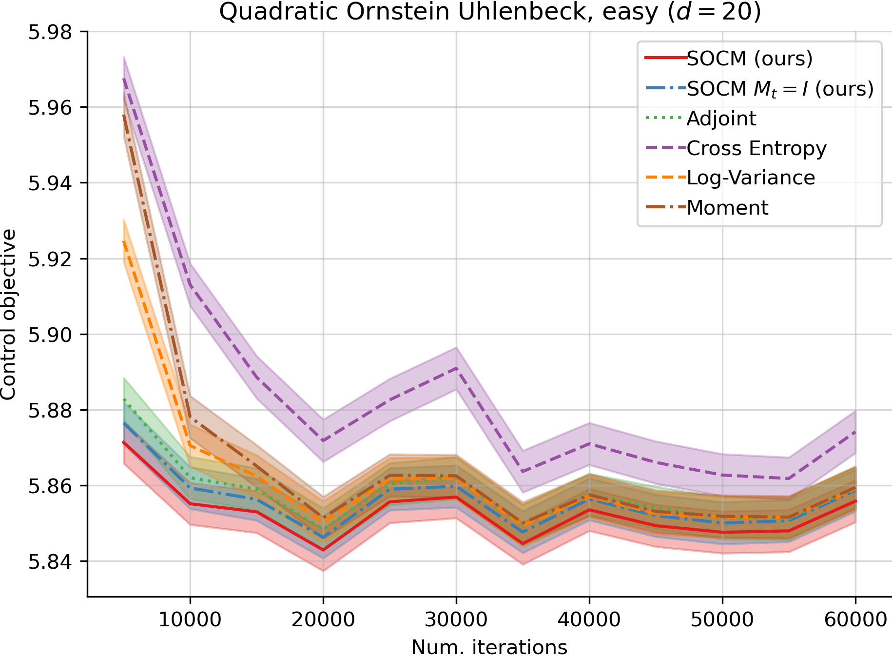
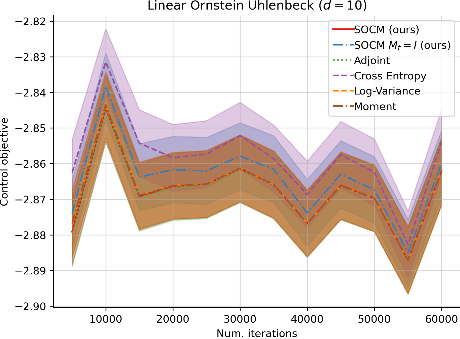
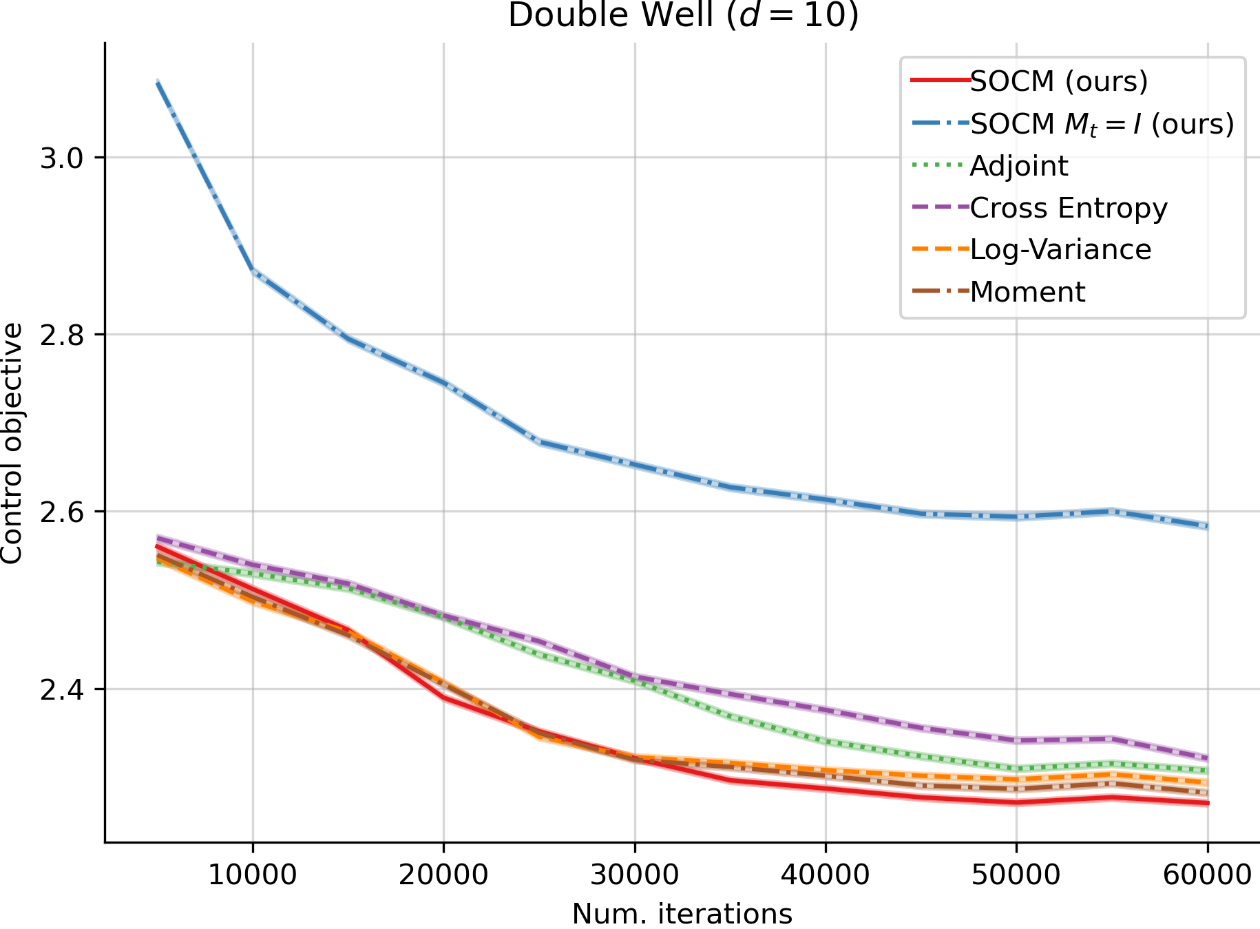
Figure 4: Plots of the control objective for the four settings.

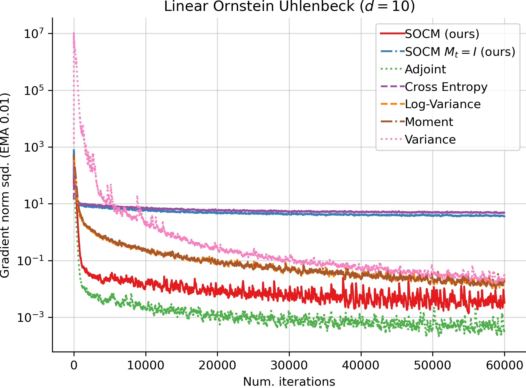
Figure 5: Plots of the norm squared of the gradient for the Linear Ornstein Uhlenbeck and Double Well settings.

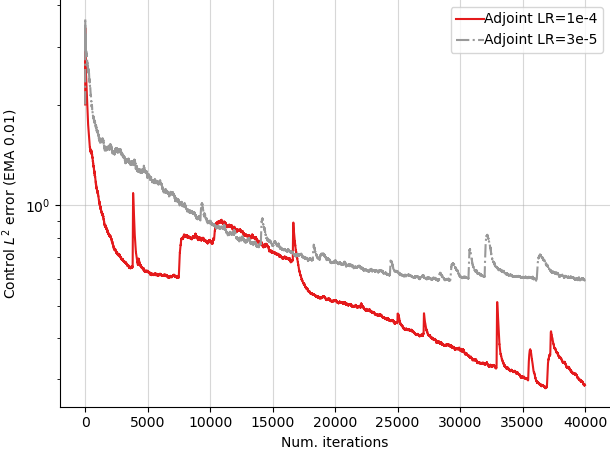
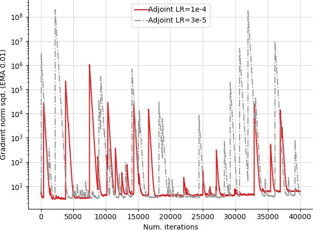
Figure 6: Plots of the control $L^{2}$ error and the norm squared of the gradient for the adjoint method on Double Well, for two different values of the Adam learning rate. The instabilities of the adjoint method persist for small learning rates, signaling an inherent issue with the loss.

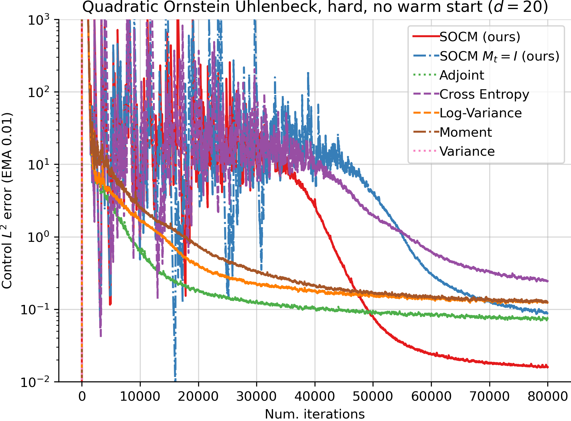
Figure 7: Plots of the control $L^{2}$ error, the norm squared of the gradient, and the control objective for the Quadratic Ornstein-Uhlenbeck (hard) setting, without using warm-start.

References

- Albergo and Vanden-Eijnden [2022] M. S. Albergo and E. Vanden-Eijnden. Building normalizing flows with stochastic interpolants, 2022.
- Albergo et al. [2023] M. S. Albergo, N. M. Boffi, and E. Vanden-Eijnden. Stochastic interpolants: A unifying framework for flows and diffusions. arXiv preprint arXiv:2303.08797, 2023.
- Baňas et al. [2022] L. Baňas, H. Dawid, T. A. Randrianasolo, J. Storn, and X. Wen. Numerical approximation of a system of hamilton–jacobi–bellman equations arising in innovation dynamics. Journal of Scientific Computing, 92, 2022.
- Beck et al. [2018] C. Beck, S. Becker, P. Grohs, N. Jaafari, and A. Jentzen. Solving stochastic differential equations and Kolmogorov equations by means of deep learning. arXiv:1806.00421, 2018.
- Beck et al. [2019] C. Beck, F. Hornung, M. Hutzenthaler, A. Jentzen, and T. Kruse. Overcoming the curse of dimensionality in the numerical approximation of Allen-Cahn partial differential equations via truncated full-history recursive multilevel Picard approximations. arXiv:1907.06729, 2019.
- Becker et al. [2019] S. Becker, P. Cheridito, and A. Jentzen. Deep optimal stopping. Journal of Machine Learning Research, 20, 2019.
- Belloni et al. [2016] A. Belloni, L. Piroddi, and M. Prandini. A stochastic optimal control solution to the energy management of a microgrid with storage and renewables. In 2016 American Control Conference (ACC), pages 2340–2345, 2016.
- Bierkens and Kappen [2014] J. Bierkens and H. J. Kappen. Explicit solution of relative entropy weighted control. Systems & Control Letters, 72:36–43, 2014.
- Bonnans et al. [2004] J. Bonnans, E. Ottenwaelter, and H. Zidani. A fast algorithm for the two dimensional hjb equation of stochastic control. M2AN. Mathematical Modelling and Numerical Analysis. ESAIM, European Series in Applied and Industrial Mathematics, 38, 07 2004.
- Calzola et al. [2022] E. Calzola, E. Carlini, X. Dupuis, and F. Silva. A semi-Lagrangian scheme for Hamilton–Jacobi–Bellman equations with oblique derivatives boundary conditions. Numerische Mathematik, page 153, 2022.
- Carlini et al. [2020] E. Carlini, A. Festa, and N. Forcadel. A semi-Lagrangian scheme for Hamilton–Jacobi–Bellman equations on networks. SIAM J. Numer. Anal., 58(6):3165–3196, 2020.
- Carmona [2016] R. Carmona. Lectures on BSDEs, stochastic control, and stochastic differential games with financial applications, volume 1. SIAM, 2016.
- Carmona and Laurière [2021] R. Carmona and M. Laurière. Convergence analysis of machine learning algorithms for the numerical solution of mean field control and games i: The ergodic case. SIAM Journal on Numerical Analysis, 59(3):1455–1485, 2021.
- Carmona and Laurière [2022] R. Carmona and M. Laurière. Convergence analysis of machine learning algorithms for the numerical solution of mean field control and games: Ii—the finite horizon case. The Annals of Applied Probability, 32(6):4065–4105, 2022.
- Carmona et al. [2018] R. Carmona, F. Delarue, et al. Probabilistic Theory of Mean Field Games with Applications I-II. Springer, 2018.
- Chan-Wai-Nam et al. [2019] Q. Chan-Wai-Nam, J. Mikael, and X. Warin. Machine learning for semilinear PDEs. Journal of Scientific Computing, 79(3):1667–1712, 2019.
- Chaudhari et al. [2018] P. Chaudhari, A. Oberman, S. Osher, S. Soatto, and G. Carlier. Deep relaxation: partial differential equations for optimizing deep neural networks. Research in the Mathematical Sciences, 5(3):30, 2018.
- Chen et al. [2018] R. T. Q. Chen, Y. Rubanova, J. Bettencourt, and D. K. Duvenaud. Neural ordinary differential equations. In Advances in Neural Information Processing Systems, volume 31. Curran Associates, Inc., 2018.
- Debrabant and Jakobsen [2013] K. Debrabant and E. R. Jakobsen. Semi-lagrangian schemes for linear and fully non-linear diffusion equations. Mathematics of Computation, 82(283):1433–1462, 2013.
- E et al. [2017] W. E, J. Han, and A. Jentzen. Deep learning-based numerical methods for high-dimensional parabolic partial differential equations and backward stochastic differential equations. Communications in Mathematics and Statistics, 5(4):349–380, 2017.
- E et al. [2021] W. E, J. Han, and A. Jentzen. Algorithms for solving high dimensional pdes: from nonlinear monte carlo to machine learning. Nonlinearity, 35(1):278, 2021.
- Feng and Kurtz [2006] J. Feng and T. G. Kurtz. Large deviations for stochastic processes. Number 131. American Mathematical Soc., 2006.
- Fleming and Stein [2004] W. H. Fleming and J. L. Stein. Stochastic optimal control, international finance and debt. Journal of Banking & Finance, 28(5):979–996, 2004.
- Gobet [2016] E. Gobet. Monte-Carlo methods and stochastic processes: from linear to non-linear. CRC Press, 2016.
- Gobet et al. [2005] E. Gobet, J.-P. Lemor, X. Warin, et al. A regression-based Monte Carlo method to solve backward stochastic differential equations. The Annals of Applied Probability, 15(3):2172–2202, 2005.
- Gómez et al. [2014] V. Gómez, H. J. Kappen, J. Peters, and G. Neumann. Policy search for path integral control. In Joint European Conference on Machine Learning and Knowledge Discovery in Databases, pages 482–497. Springer, 2014.
- Gorodetsky et al. [2018] A. Gorodetsky, S. Karaman, and Y. Marzouk. High-dimensional stochastic optimal control using continuous tensor decompositions. International Journal of Robotics Research, 37(2-3), 3 2018.
- Greif [2017] C. Greif. Numerical methods for hamilton-jacobi-bellman equations. 2017.
- Han and Hu [2020] J. Han and R. Hu. Deep fictitious play for finding markovian nash equilibrium in multi-agent games. In Mathematical and scientific machine learning, pages 221–245. PMLR, 2020.
- Han et al. [2018] J. Han, A. Jentzen, and W. E. Solving high-dimensional partial differential equations using deep learning. Proceedings of the National Academy of Sciences, 115(34):8505–8510, 2018.
- Hartmann and Schütte [2012] C. Hartmann and C. Schütte. Efficient rare event simulation by optimal nonequilibrium forcing. Journal of Statistical Mechanics: Theory and Experiment, 2012(11):P11004, 2012.
- Hartmann et al. [2014] C. Hartmann, R. Banisch, M. Sarich, T. Badowski, and C. Schütte. Characterization of rare events in molecular dynamics. Entropy, 16(1):350–376, 2014.
- Hartmann et al. [2017] C. Hartmann, L. Richter, C. Schütte, and W. Zhang. Variational characterization of free energy: Theory and algorithms. Entropy, 19(11), 2017.
- Hartmann et al. [2019] C. Hartmann, O. Kebiri, L. Neureither, and L. Richter. Variational approach to rare event simulation using least-squares regression. Chaos: An Interdisciplinary Journal of Nonlinear Science, 29(6):063107, 2019.
- Ho et al. [2020] J. Ho, A. Jain, and P. Abbeel. Denoising diffusion probabilistic models. In Advances in Neural Information Processing Systems, volume 33. Curran Associates, Inc., 2020.
- Holdijk et al. [2023] L. Holdijk, Y. Du, F. Hooft, P. Jaini, B. Ensing, and M. Welling. Stochastic optimal control for collective variable free sampling of molecular transition paths, 2023.
- Hutton and Nelson [1984] J. E. Hutton and P. I. Nelson. Interchanging the order of differentiation and stochastic integration. Stochastic Processes and their Applications, 18(2):371–377, 1984.
- Hutzenthaler and Kruse [2020] M. Hutzenthaler and T. Kruse. Multilevel picard approximations of high-dimensional semilinear parabolic differential equations with gradient-dependent nonlinearities. SIAM Journal on Numerical Analysis, 58(2):929–961, 2020.
- Hutzenthaler et al. [2016] M. Hutzenthaler, A. Jentzen, T. Kruse, et al. Multilevel picard iterations for solving smooth semilinear parabolic heat equations. arXiv preprint arXiv:1607.03295, 2016.
- Hutzenthaler et al. [2018] M. Hutzenthaler, A. Jentzen, T. Kruse, T. A. Nguyen, and P. von Wurstemberger. Overcoming the curse of dimensionality in the numerical approximation of semilinear parabolic partial differential equations. arXiv:1807.01212, 2018.
- Hutzenthaler et al. [2019] M. Hutzenthaler, A. Jentzen, and T. Kruse. Overcoming the curse of dimensionality in the numerical approximation of parabolic partial differential equations with gradient-dependent nonlinearities. arXiv:1912.02571, 2019.
- Jensen and Smears [2013] M. Jensen and I. Smears. On the convergence of finite element methods for hamilton–jacobi–bellman equations. SIAM Journal on Numerical Analysis, 51(1):137–162, 2013.
- Kappen [2005] H. J. Kappen. Path integrals and symmetry breaking for optimal control theory. Journal of Statistical Mechanics: Theory and Experiment, 2005(11), nov 2005.
- Kappen and Ruiz [2016] H. J. Kappen and H. C. Ruiz. Adaptive importance sampling for control and inference. Journal of Statistical Physics, 162(5):1244–1266, 2016.
- Kappen et al. [2012] H. J. Kappen, V. Gómez, and M. Opper. Optimal control as a graphical model inference problem. Machine learning, 87(2):159–182, 2012.
- Karatzas and Shreve [1991] I. Karatzas and S. Shreve. Brownian Motion and Stochastic Calculus. Graduate Texts in Mathematics (113) (Book 113). Springer New York, 1991.
- Li et al. [2020] X. Li, T.-K. L. Wong, R. T. Chen, and D. Duvenaud. Scalable gradients for stochastic differential equations. In International Conference on Artificial Intelligence and Statistics, pages 3870–3882. PMLR, 2020.
- Lipman et al. [2022] Y. Lipman, R. T. Q. Chen, H. Ben-Hamu, M. Nickel, and M. Le. Flow matching for generative modeling, 2022.
- Liu et al. [2023] G.-H. Liu, Y. Lipman, M. Nickel, B. Karrer, E. A. Theodorou, and R. T. Q. Chen. Generalized schrödinger bridge matching, 2023.
- Ma and Ma [2020] J. Ma and J. Ma. Finite difference methods for the hamilton-jacobi-bellman equations arising in regime switching utility maximization. J. Sci. Comput., 85(3):55, 2020.
- Mitter [1996] S. K. Mitter. Filtering and stochastic control: A historical perspective. IEEE Control Systems Magazine, 16(3):67–76, 1996.
- Munos et al. [2016] R. Munos, T. Stepleton, A. Harutyunyan, and M. Bellemare. Safe and efficient off-policy reinforcement learning. In Advances in Neural Information Processing Systems, volume 29. Curran Associates, Inc., 2016.
- Nüsken and Richter [2021] N. Nüsken and L. Richter. Solving high-dimensional Hamilton–Jacobi–Bellman pdes using neural networks: perspectives from the theory of controlled diffusions and measures on path space. Partial differential equations and applications, 2:1–48, 2021.
- Oksendal [2013] B. Oksendal. Stochastic differential equations: an introduction with applications. Springer Science & Business Media, 2013.
- Onken et al. [2023] D. Onken, L. Nurbekyan, X. Li, S. W. Fung, S. Osher, and L. Ruthotto. A neural network approach for high-dimensional optimal control applied to multiagent path finding. IEEE Transactions on Control Systems Technology, 31(1):235–251, jan 2023.
- Pavliotis [2014] G. A. Pavliotis. Stochastic processes and applications: diffusion processes, the Fokker-Planck and Langevin equations, volume 60. Springer, 2014.
- Pham [2009] H. Pham. Continuous-time stochastic control and optimization with financial applications, volume 61. Springer Science & Business Media, 2009.
- Pontryagin [1962] L. Pontryagin. The Mathematical Theory of Optimal Processes. Interscience Publishers, 1962.
- Pooladian et al. [2023] A.-A. Pooladian, H. Ben-Hamu, C. Domingo-Enrich, B. Amos, Y. Lipman, and R. T. Q. Chen. Multisample flow matching with optimal transport couplings. In International Conference on Machine Learning, 2023.
- Powell and Meisel [2016] W. B. Powell and S. Meisel. Tutorial on stochastic optimization in energy—part i: Modeling and policies. IEEE Transactions on Power Systems, 31(2):1459–1467, 2016.
- Rawlik et al. [2013] K. Rawlik, M. Toussaint, and S. Vijayakumar. On stochastic optimal control and reinforcement learning by approximate inference. In Twenty-Third International Joint Conference on Artificial Intelligence, 2013.
- Reich [2019] S. Reich. Data assimilation: The Schrödinger perspective. Acta Numerica, 28:635–711, 2019.
- Rezende and Mohamed [2015] D. Rezende and S. Mohamed. Variational inference with normalizing flows. In Proceedings of the 32nd International Conference on Machine Learning, 2015.
- Ronneberger et al. [2015] O. Ronneberger, P. Fischer, and T. Brox. U-net: Convolutional networks for biomedical image segmentation. In Medical Image Computing and Computer-Assisted Intervention–MICCAI 2015: 18th International Conference, Munich, Germany, October 5-9, 2015, Proceedings, Part III 18, pages 234–241. Springer, 2015.
- Rubinstein and Kroese [2013] R. Y. Rubinstein and D. P. Kroese. The cross-entropy method: a unified approach to combinatorial optimization, Monte-Carlo simulation and machine learning. Springer Science & Business Media, 2013.
- Song and Ermon [2019] Y. Song and S. Ermon. Generative modeling by estimating gradients of the data distribution. arXiv preprint arXiv:1907.05600, 2019.
- Song et al. [2021] Y. Song, J. Sohl-Dickstein, D. P. Kingma, A. Kumar, S. Ermon, and B. Poole. Score-based generative modeling through stochastic differential equations. In International Conference on Learning Representations (ICLR 2021), 2021.
- Theodorou et al. [2011] E. Theodorou, F. Stulp, J. Buchli, and S. Schaal. An iterative path integral stochastic optimal control approach for learning robotic tasks. IFAC Proceedings Volumes, 44(1):11594–11601, 2011. 18th IFAC World Congress.
- Van Handel [2007] R. Van Handel. Stochastic calculus, filtering, and stochastic control. Course notes, URL http://www. prince- ton. edu/rvan/acm217/ACM217, 2007.
- Villani [2003] C. Villani. Topics in Optimal Transportation. Graduate studies in mathematics. American Mathematical Society, 2003.
- Villani [2008] C. Villani. Optimal Transport: Old and New. Grundlehren der mathematischen Wissenschaften. Springer Berlin Heidelberg, 2008.
- Zhang et al. [2004] J. Zhang et al. A numerical scheme for BSDEs. The annals of applied probability, 14(1):459–488, 2004.
- Zhang and Chen [2022] Q. Zhang and Y. Chen. Path integral sampler: A stochastic control approach for sampling. In International Conference on Learning Representations, 2022.
- Zhang et al. [2014] W. Zhang, H. Wang, C. Hartmann, M. Weber, and C. Schütte. Applications of the cross-entropy method to importance sampling and optimal control of diffusions. SIAM Journal on Scientific Computing, 36(6):A2654–A2672, 2014.
- Zhou et al. [2021] M. Zhou, J. Han, and J. Lu. Actor-critic method for high dimensional static Hamilton–Jacobi–Bellman partial differential equations based on neural networks. SIAM Journal on Scientific Computing, 43(6):A4043–A4066, 2021.