Model parameter optimisation with Bayesian statistics

Abstract

The accuracy and precision of models are key issues for the design and development of new applications and experiments. We present a method of optimisation for a large variety of models. This approach is designed in order both to improve the accuracy of models through the modification of free parameters of these models, which results in a better reproduction of experimental data, and to estimate the uncertainties of these parameters and, by extension, their impacts on the model output. We discuss the method in detail and present a proof-of-concept for Monte Carlo models.

1 Introduction

As the Dutch physicist Walter Lewin wisely said: “Any measurement that you make, without any knowledge of the uncertainty, is meaningless”. It is true for experimental measurements as well as for theoretical models. As precise and reliable as they can be, experimental data and models are always only an approximation of the reality and, therefore, the difference between data or models predictions on the one hand and the reality on the other hand have to be estimated to make them meaningful. However, while the estimation of uncertainties for experimental measurements became the norm a century ago, the evaluation of model uncertainties is much more recent and was a long time limited to the consideration of statistical uncertainties only.

The improvement of computing power in the last decades allowed the development of new tools for model uncertainty quantification, especially for Monte Carlo (MC) models. Such models are of the highest importance in the field of nuclear physics as measuring all required nuclear data is impossible for all the various fields of application (e.g., fusion technology, medical hadron therapy, cosmogenic nuclide production, transmutation of nuclear waste, etc.). Models able to predict the relevant data are needed to design instruments, for radioprotection, or simply to analyse data. The critical aspects in nuclear physics initiated from a very early time the study of model uncertainties, which is commonly called nuclear data evaluation. Considering the wide range of applications of nuclear models and their relevance for societies, it is obvious that model calculations must be as precise and reliable as possible. Consequently, the bias, i.e., the difference between the estimator and the true value of an observable, and the uncertainties of models must be estimated precisely for a proper use of these nuclear models.

The majority of the methods proposed for the study of model uncertainties is based on Bayesian statistics. Bayesian statistics is a general framework for inference where limited knowledge about quantities is expressed in terms of probability distributions. The object of central interest in Bayesian inference is the posterior distribution, which represents an updated state of knowledge taking into account observations (entering the likelihood) and prior knowledge. This allows to estimate the likelihood of a result as well as its uncertainties.

In the 20th century, nuclear data evaluation was mostly focussed on energy domains relevant for nuclear power plants. Namely, nuclear data evaluations focussed on neutron projectiles with energies below 20 MeV. This led to the creation of nuclear data libraries, which are basically tables of (double differential) cross sections. At present, new types of projects are envisaged with much higher operating energies and with more types of projectile particles. As an example, the Multi-purpose hYbrid Research Reactor for High-tech Applications (MYRRHA [1]) project will operate at energies up to 600 MeV. Therefore, a new (and large) energy range must be carefully studied.

During the European Nuclear Data project CHANDA [2], and more recently in the SANDA [3] project, an important effort has been devoted to the development, improvement, and validation of high energy nuclear models, in particular the INCL/ABLA combination of models that are now widely used for high energy applications.

In the CHANDA project [2], for the first time, a study had been conducted to investigate a possible methodology based on the Bayesian framework for quantifying the uncertainties linked to parameters in high energy models, which could then possibly be taken into account in MC transport codes [4]. In the present study, which was included in the SANDA project [3], it is proposed to investigate if the methodology we developed can be applied to a large number of parameters used in the INCL model and if the methodology can be applied within a reasonable computational time. We are interested in the model combination of the IntraNuclear Cascade model of Liège (INCL++6) [5] and the de-excitation model ABLA++[6, 7]. In combination, they are able to simulate spallation reactions, which are high-energy nuclear reactions, in which a target nucleus is hit by an incident particle of energy greater than some tens of MeV and up to a few GeV.

Noteworthy, the objectives of this study (see section 2) are specific to nuclear data evaluation using the combination INCL/ABLA. However, the methodology developed to study our specific case is a general framework that can be applied to a large variety of models. In section 3, the basics of the method is discussed together with the requirements and the limits of our approach. section 4 presents the treatment of experimental data required before the use of the algorithm. Next, the methodology is applied to INCL/ABLA with the use of real experimental data in section 5. Finally, we discuss the outlook of this work in section 6.

2 Objective

In the framework of the European project SANDA [3], we developed a new method able (1) to estimate the optimal parameters for a model and (2) to estimate the uncertainties of these parameters. In this study, our objectives are twofold. First, we aim at demonstrating the feasibility of our approach for real cases using the combination of Monte Carlo models INCL (for the simulation of the intranuclear cascade) and ABLA (for the simulation of the de-excitation of nuclei). Second, we study the possibilities, the difficulties, and the limits of our procedure both for the evaluation of the optimal parameters of a model and for the evaluation of the corresponding uncertainties.

Model bias is, by definition, the expected difference between model predictions and the true values of the corresponding observables (e.g., neutron multiplicity, angular distribution, mass distribution, etc.). Equally, the bias of the model parameters is the expected difference between the parameter values provided to the model and their true values. However, the “true” values of the parameters (when it is meaningful) are not known and are not accessible. Therefore, we have to rely on experimental data to characterise the model bias and the parameter bias. This is a reasonable consideration because there is no a priori reason for the experimental data to over- or underestimate the reality. In other words, experimental data are the best a priori estimate of the reality available and are a priori unbiased. This can be written in an equation:

$$Bias=\operatorname*{\mathbb{E}}(\sigma_{exp}-\sigma_{true})=0,$$ (1)

with $\sigma_{exp}$ experimental data and $\sigma_{true}$ the true values of the corresponding observables.

One conceptual issue for determining parameter bias is that the definition of the bias is meaningless when the parameters are not “physical” parameters. As an example, particles masses are “physical” parameters, while parameters used in INCL to determine when the model stops running are model dependent parameters. Additionally, estimating parameter bias will be done within the Bayesian framework, which assumes that the combination INCL/ABLA is a perfect model. In other words, the Bayesian procedure assumes that the “correct” choice of parameter values will lead to predictions that perfectly coincide with the true values. However, as says the famous quote attributed to the British statistician George E.P. Box: “All models are wrong, but some are useful”. INCL/ABLA, as any model, cannot be perfect, even with the “correct” parameters. This is why the procedure will not search for the true value of the model parameters but for the optimal parameters within the context of the model considered and of the observables studied. Additionally, the imperfection of our model may lead to unreasonable values for certain parameters with respect to our a priori knowledge. Such a case can be interpreted as a missing mechanism, an incorrect hypothesis, or a constrain not properly taken into account in the model and therefore might be used to improve the physics of the model.

On the other hand, the uncertainties of the model parameters will also be evaluated. These uncertainties are useful as they provide information about the error propagation in the model. Small uncertainties for a given parameter would indicate that a small modification significantly modify model predictions. Reciprocally, large uncertainties would indicate that the model outcome is not very sensitive to the exact choice of this parameter.

3 Methodology

As mentioned in section 2, the objectives of the method we developed is to estimate the optimal model parameters and the uncertainties associated to these parameters, the latter would provide information about the error propagation in the model. The related question of the model bias and of the estimation of model uncertainties is orthogonal to this study and has already been addressed in a previous study carried out by Schnabel within the CHANDA framework [8] and will therefore not be discussed any further. However, these complementary questions must be both addressed for a complete study.

The methodology we developed is based on the Generalised Least Squares (GLS) method [9], which is an important technique in nuclear data evaluation. The GLS is often used to estimate the unknown parameters in a linear regression model, which takes into account the correlations between observed data. The GLS is a method of regression similar to the common $\chi^{2}$ method but the correlations are taken into account. Additionally, the a priori values for the model parameters are treated as extra data, which limits the risk of unphysical predictions for the parameters.

Our approach is divided into two main parts.

In a first step, we want to know what are the optimal parameters for the model, i.e., we want to estimate what are the parameters that will result in the best model predictions (i.e., the parameter set that will maximise the likelihood of the model). Our approach, being based on Bayesian statistics, takes into account both, the reproduction of the experimental data and the a priori knowledge about the parameters. To this end, we employ an iterative algorithm for maximum likelihood estimation that exploits a specific structure of the likelihood and is inspired from the Expectation Maximisation (EM) method [10]. As with the EM, our algorithm alternates between an expectation step, in which we create the expectation of the likelihood as a function of the parameter set used, and the maximisation step computing the parameter set maximising the likelihood. We will call this part of our method the Expectation Maximisation phase.

In the second step, we want to know what are the uncertainties associated with each parameter.For this step, we developed an approach based on Gibbs sampling, which is suitable for stochastic models. With this approach, we sample parameter sets in a multivariate normal distribution using the posterior covariance matrix of the model. The distribution of the parameters at the end of this second step allows to determine the uncertainties of these parameters. Once again, we will call this part of our method the Gibbs sampling phase, through the term is not strictly correct

It is important to mention that, if the model has difficulties reproducing some of the experimental data with respect to their error bars, the algorithm will focus on these data points and neglect others. This is why the selection of experimental data to be included in the analysis as well as a careful study of their uncertainties must be carried out before trying to optimise the model parameters. The experimental data included in this approach have to be reasonably reproducible by the model. Otherwise, these toxic data may jeopardise finding reasonable estimates for the parameter values.

3.1 Optimisation algorithm

In the EM method and in Gibbs sampling, an iterative algorithm is employed. The number of iterations for both methods is a free parameters, which needs to be specified by the user. For the EM algorithm, it must be large enough that the approach converges to the optimal parameter set. For the Gibbs sampling, it must be large enough to estimate the variance of the parameters using the distribution of the parameter set produced. On the other hand, the computational time increases linearly with the number of iterations. Therefore, the minimum number of iterations required might range from a few tens to a hundred for the EM and from a few hundreds to a few thousands for the Gibbs sampling.

The main idea of the EM is as follows. We start with a model $\mathcal{M}$ (here INCL/ABLA), experimental data $\vec{\sigma}_{exp}$, and a set of parameters $\vec{p}_{ref}$, which represents the best estimate of these parameters a priori (i.e., without knowledge of $\vec{\sigma}_{exp}$). Here, the model is seen as a function taking a vector as input (the parameters) and producing a vector as an output (the observables) corresponding to the experimental data. This means that the dimension of the model predictions, $\mathcal{M}(\vec{p})$, must be the same as the dimension of $\vec{\sigma}_{exp}$. In our specific case of INCL/ABLA, this is done by using an additional layer above the standard version of the model. This extra layer extracts the experimental setups (projectiles, targets, energies, angles, etc.) from the experimental data, runs the INCL/ABLA simulations with the same setups and, using the parameter set $\vec{p}$, extracts the calculated observables corresponding to the experimental data from the standard INCL/ABLA output produced and, finally, produces a vector matching $\vec{\sigma}_{exp}$.

Next, we enter a loop to improve the set of parameters $\vec{p}_{ref}$. After the i-th iteration of the loop, the improved set of parameters is called $\vec{p}_{i}$. With the knowledge of how the model varies locally, which is given by the Jacobian (also called the sensitivity matrix) of the model evaluated at $\vec{p}_{i}$, and the difference between the model prediction $\mathcal{M}(\vec{p}_{i})$ and the experimental data $\vec{\sigma}_{exp}$, one can determine the best set of parameters $\vec{p}_{i+1}$ to minimise the difference between the model and the experimental data, assuming the model is linear between $\vec{p}_{i}$ and $\vec{p}_{i+1}$. Since the model is likely not strictly linear, the new set of parameters will most likely not be the optimal parameter set. However, as long as the model is not completely erratic between $\vec{p}_{i}$ and $\vec{p}_{i+1}$, the linearisation of the model can be seen as an acceptable approximation. Therefore, the new set of parameters $\vec{p}_{i+1}$ will likely be an improvement with respect to $\vec{p}_{i}$. Then, we can reevaluate the local Jacobian and the real model prediction in $\vec{p}_{i+1}$ and restart the loop until convergence of $\vec{p}$.

Explicitly, the EM is executed as follows. At the beginning of each loop, we linearise the model using a Taylor series approximation in $\vec{p}_{i}$:

$$\vec{T_{i}}(\vec{p})=\mathcal{M}(\vec{p}_{i})+J_{p_{i}}\times(\vec{p}-\vec{p}_{i}),$$ (2)

with the Jacobian matrix $J_{p_{i}}$ of the model evaluated at $\vec{p}_{i}$:

$$J_{p_{i}}=\frac{d\mathcal{M}(\vec{p}_{i})}{\vec{dp_{i}}}.$$ (3)

We introduce the matrix $J_{i}$:

$$J_{i}=\left(\begin{matrix}\mathbb{I}_{n\times n}&J_{p_{i}}\\ \emptyset&\mathbb{I}_{m\times m}\\ \end{matrix}\right),$$ (4)

with $n$ the number of experimental data, $m$ the number of parameters, and $\mathbb{I}$ the identity matrix.

The definition of $J_{i}$ allows to define the matrix of regression as:

$$\tilde{\Sigma}_{i}=J_{i}\ \Sigma\ J_{i}^{T}=\left(\begin{matrix}\tilde{\Sigma}_{DD_{i}}&\tilde{\Sigma}_{DI_{i}}\\ \tilde{\Sigma}_{ID_{i}}&\tilde{\Sigma}_{II_{i}}\\ \end{matrix}\right),$$ (5)

with $\tilde{\Sigma}_{DD_{i}}$ of dimension ${n\times n}$, $\tilde{\Sigma}_{II_{i}}$ of dimension ${m\times m}$, and $\Sigma$ the covariance matrix of the joint distribution of the experimental data and the input parameters:

$$\Sigma=\left(\begin{matrix}\Sigma_{exp}&\emptyset\\ \emptyset&\Sigma_{p}\\ \end{matrix}\right),$$ (6)

with $\Sigma_{exp}$ and $\Sigma_{p}$ the covariance matrix of the experimental data and of the parameters, respectively. The $\Sigma$ matrices might be non-diagonal in case of correlations between either the experimental data or the parameters.

Next, we can determine an improved set of parameters using the formula of the GLS method:

$$\vec{p}\mkern 2.0mu\vphantom{p}^{\prime}=\vec{p}_{ref}+\tilde{\Sigma}_{ID_{i}}\left(\tilde{\Sigma}_{DD_{i}}\right)^{-1}\left[\vec{\sigma}_{exp}-\vec{T_{i}}(\vec{p}_{ref})\right].$$ (7)

The derivation of this formula is given in Appendix A.

This formula would provide directly the optimal parameters ($\vec{p}_{op}$) for the model in case the model is linear. However, in general, $\vec{p}\mkern 2.0mu\vphantom{p}^{\prime}$ is only an approximation of $\vec{p}_{op}$. The quality of this approximation is directly correlated to the linearity of the model between $\vec{p}_{i}$ and $\vec{p}_{op}$. Even if the model is not linear, $\vec{p}\mkern 2.0mu\vphantom{p}^{\prime}$ is likely an improvement with respect to $\vec{p}_{i}$. Next, we can restart the procedure with $\vec{p}_{i+1}=\vec{p}\mkern 2.0mu\vphantom{p}^{\prime}$. This will improve the quality of the GLS hypothesis of a linear model between $\vec{p}_{i}$ and $\vec{p}_{op}$ and therefore, the precision of Equation 7. If the model is not completely erratic, we expect the difference $|\vec{p}_{op}-\vec{p}_{i}|$ to decrease quickly with the number of iterations.

For a stochastic model, the hypothesis of linearity between $\vec{p}_{i}$ and $\vec{p}_{op}$ might be reasonable as long as the expected difference of the model predictions between $\vec{p}_{i}$ and $\vec{p}_{op}$ dominates the stochasticity. However, as $\vec{p}_{i}$ approaches $\vec{p}_{op}$, Equation 7 becomes less and less valid. Therefore, we expect an initial quick convergence as $\vec{p}_{i}$ is far from $\vec{p}_{op}$, then $\vec{p}_{i}$ will start oscillating around $\vec{p}_{op}$. In order to evaluate $\vec{p}_{op}$, we average the values of $\vec{p}_{i}$ along the oscillating phase. This significantly reduces the effect of stochasticity.

In the second phase of the algorithm, the Gibbs sampling, we want to sample $\vec{p}_{i}$ around $\vec{p}_{op}$ using a multivariate normal distribution with the posterior covariance matrix $\Sigma_{i}$ in order to evaluate the distribution of $\vec{p}$ and with it, to measure the uncertainties and the correlations of the parameters:

$$\vec{p}_{i+1}=\mathcal{N}(\vec{p}\mkern 2.0mu\vphantom{p}^{\prime},\Sigma_{i+1}).$$ (8)

For each loop of the Gibbs sampling, $\vec{p}\mkern 2.0mu\vphantom{p}^{\prime}$ is re-approximated using Equation 7 (which means we process one loop of the EM within each iteration of the Gibbs sampling) and the covariance matrix $\Sigma_{i+1}$ is an updated version of the initial covariance matrix of the parameters (see Appendix A for details), which includes the variance of the experimental data and the error propagation through the model:

$$\Sigma_{i+1}=\Sigma_{p}-\tilde{\Sigma}_{ID_{i}}\left(\tilde{\Sigma}_{DD_{i}}\right)^{-1}\tilde{\Sigma}_{DI_{i}}.$$ (9)

This Gibbs sampling is well suited in the case of stochastic models since the $\vec{p}\mkern 2.0mu\vphantom{p}^{\prime}$ used is re-approximated in each loop and its dispersion over the loops allows to integrate the stochasticity of the model into the uncertainties of the parameters. In addition to the dispersion of $\vec{p}\mkern 2.0mu\vphantom{p}^{\prime}$, the sampling uses the updated covariance matrix $\Sigma_{i+1}$, which contains the information of the a priori knowledge about the parameters and the experimental data. It also contains information about the error propagation through the model. These uncertainties (and the correlations between the parameters) can be obtained from the covariance matrix of the multivariate distribution of $\vec{p}_{i}$ obtained with the Gibbs sampling. This allows to evaluate the parameter uncertainties in the Bayesian framework taking into account the a priori uncertainties of these parameters as well as other relevant uncertainties, which are the error propagation through the model, the stochasticity of the model (which depends on the statistic used), and the uncertainties of the experimental data. On the other hand, if we do not want to incorporate the information about the stochasticity of the model into the uncertainties of the parameters, we can average the covariance matrix $\Sigma_{i}$ over the iterations. In this case we would obtain parameters uncertainties with only the consideration of a priori uncertainties of these parameters, a priori uncertainties of the experimental data used, and the error propagation through the model.

3.2 CPU Optimisation

To reduce calculation time, some CPU optimisations have been applied.

First, concerning the inversion of the matrix $\tilde{\Sigma}_{DD_{i}}$, which is very CPU time consuming when using a large amount of experimental data, the Woodbury matrix identity is used:

$$\left(\tilde{\Sigma}_{DD_{i}}\right)^{-1}=\left(\Sigma_{exp}+J_{p}\Sigma_{p}J_{p}^{T}\right)^{-1}$$

$$=\Sigma_{exp}^{-1}-\Sigma_{exp}^{-1}\ J_{p}\ \left(\Sigma_{p}^{-1}+J_{p}^{T}\Sigma_{exp}^{-1}J_{p}\right)^{-1}J_{p}^{T}\Sigma_{exp}^{-1}.$$ (10)

When no correlation is considered, i.e., when the $\Sigma$ matrices are diagonal, the inversion is straightforward. When there are correlations, they are often limited to a small group of data and the inversion of the matrix can still be efficiently performed. Consequently, the problem of a large non-diagonal matrix inversion becomes a problem of large matrix multiplications, which is faster and can easily be parallelised.

Second, theoretically the Jacobian should be computed for each loop. However, this would be highly CPU inefficient as the Jacobian does not change drastically between two loops while the new calculation would require a significant CPU time. Therefore, at the end of each iteration, we check if the Jacobian is still valid and, if not, only then it is revaluated. This is done with a comparison of $\mathcal{M}(\vec{p}_{i})$ (which is evaluated in each loop for the needs of the Taylor approximation) and $T_{j}(\vec{p}_{i})$, the Taylor approximation performed the last time the Jacobian has been evaluated. If the predictions based on the exact model and the linearisation at $\vec{p}_{i}$ differ by less than a predefined value, we consider the Jacobian as still valid. In practice, we decided to update the Jacobian only when the prediction of the Taylor approximation differs by more than twice the best relative prediction ever obtained with a Taylor approximation. E.g., if the best prediction was able to predict the model output within 20% accuracy, we conserve the current Jacobian until the Taylor approximation differs by more than 40% with the model output.

Third, since we assemble values expressed in different units in the $\Sigma$ matrix and, by extension, the $\tilde{\Sigma}_{i}$ matrices, it is not rare to have matrix elements that differ by many orders of magnitude. This can introduce errors due to the limited precision of computers while multiplying or inverting the matrices. In such a case, it is useful to rescale the output of the model and the experimental data. In other words, we can choose to optimise the parameters for the model $\mathcal{M}^{\prime}=A\times\mathcal{M}$ using the experimental data $\tau^{\prime}=A\times\tau$ with $A$ an arbitrary diagonal matrix. In such a case, the experimental error bars must be updated but not the parameters and their uncertainties. Proceeding this way is perfectly equivalent to optimise the parameters for the model $\mathcal{M}$ using the experimental data $\tau$.

3.3 Limits of the approach

In our case, in which we use INCL/ABLA, there are three main limits for the use of the method.

First, one of the main challenges with nuclear data evaluation is the large number of observables to reproduce. One crucial assumption concerns the uncertainties of the experimental data. Including automatically a large number of experimental data sets into the Bayesian procedure always bears the risk that some data sets have too low uncertainties assigned. It is often the case with old experimental data for which systematic errors were often not evaluated or roughly set to 10%. As an example, some of the experimental data included in our study had relative uncertainties below 1%. In this case, the Bayesian procedure attributes a very high importance to this data while other data measured in experiments with a more rigorous uncertainty evaluation will contribute less than they should to the final results. Therefore, a careful study of the experimental data that are included in the Bayesian procedure must be carried out in order to use realistic (or, at least, consistent) uncertainties for every set of data. This is further discussed in section 4.

Similarly, a large number of data for some experiments will lead to over fitting these data, because each data point is considered individually and not as a set of data. This is because most data sets almost never provide correlations. In other words, the more data points an experiment has, the more it will influence the final result of the study. For example, the neutron production cross section has been much more intensively studied than the proton production cross section. Therefore, if the two data sets are included in the same study, the neutron production cross sections will have much more weight for the final results than the proton production cross sections, simply because there are much more data of the former than of the latter.

The second main issue is about the stochasticity of the model used. The energy considered (above 20 MeV) is not described properly with deterministic models as the number of possibilities increases exponentially with energy. MC models become necessary for these energies but it comes with the usual balance between precision and computation time. However, no matter how good the statistics is, two simulations with the same initial state but different random seeds will give different results. In order to avoid that the a posteriori probability associated to a parameter set varies too much from one run to another, the statistics must be carefully chosen in order to obtain a good balance between CPU time and precision. This might become complex for cases with a large number of different experimental data requiring very different statistics to be properly estimated by the model.

Finally, model deficiencies are not taken into account. Parameters can be optimised within the context of the model but the approach does not provide direct information about model deficiencies. This has two consequences: First, if the model deficiencies forbid to reproduce the experimental data whatever the parameter set used, the estimated optimal set will be unsatisfactory. As an example, if we try to optimise the parameters of a toy model in which the data to be reproduced are distributed as a quadratic function and the toy model allows only linear functions, the approach will optimise the parameter to minimise the bias but, despite the parameter being optimal, the model will not be able to reproduce the quadratic shape of experimental data (see ref. [4], section 3.2). Second, as the approach minimises the variance, which evolves with the square of the difference between experimental data and model predictions, a minor improvement in a region where the model is highly deficient will be seen as a great improvement, while a large increase of the difference between experimental data and the model predictions in regions where the model reproduce the experimental data properly will only be seen as a minor deterioration of the model. To summarise, if we try to optimise the model using experimental data with parts of them in deficient regions of the model and another part in efficient regions of the model, the algorithm will primarily improve the model prediction in the worst regions regardless of the effects that this produces on the model predictions in the good regions. In order to be complete, the quantification of the reliability of the model hypotheses should be done in a “global” study, i.e., by accounting for all the available data for which a given parameter plays a role.

4 Experimental data treatment

As discussed in subsection 3.3, including a large amount of experimental data coming from a large number of experiments, teams, and from different decades, is very problematic as the quality of the data often differs relative to each others. Actually, the main problem with experimental data is not with their accuracy but with their experimental error bars, which are crucial in our analysis as they define the covariance matrix $\Sigma$. Sometimes, these error bars are not representative of the real accuracy and precision of the experimental data. Additionally, the error bars were sometimes not evaluated consistently for all experimental data. Some can be pure statistical error bars, while others includes systematic errors, themselves implying a more or less thorough analysis of the experimental setup by the experimenters. It is obvious that some of the given error bars are badly evaluated when two (or more) experimental data sets exclude each other by several $\sigma$. This issue has partly been addressed by Schnabel within the CHANDA framework giving the possibility to rescale automatically experimental error bars when several data sets are available for the same observables [11]. However, there is only one set of experimental data available for most of the reactions we studied. Therefore, we need a more general approach for cases in which only one set of data is available for an observable. Unfortunately, to our knowledge, there is no mathematical approach allowing to provide systematic error bars for a set of experimental data based only on the experimental data themselves.

One possibility to overcome this problem is the application of templates that contain reasonable ranges for the uncertainty components involved, e.g., ref. [12]. However, without the availability of such templates, the only way to provide reasonable uncertainty components is by thoroughly re-analysing the details provided in the publications of the experiments or interact with the experimenters, if possible. In our case, it is not reasonable to reprocess the systematic error bars of all data sets included in our analysis. Therefore, we propose here an alternative approach taking the error bars provided with the experimental data and applying an arbitrary algorithm to normalise those error bars. This algorithm rules that experimental data with error bars too small to be realistic should be treated as experimental data with large uncertainties as there were badly evaluated. Additionally, the confidence we have in those data decreases with the increasing unlikelihood of the error bars assigned. Therefore, the algorithm uses arbitrary thresholds under which uncertainties are rescaled up to predefined levels. On the other hand, we decided to trust the realistic uncertainties provided by other experiments regardless of the differences of the uncertainty evaluation.

In practice, all relative uncertainties below 1% are considered as very unrealistic and are arbitrarily rescaled to 30%. Those between 1% and 5% are considered as unrealistic and are rescaled to 20%. Relative uncertainties between 5% and 10% are considered as realistic but likely underestimated and are rescaled to 10%. Finally, relative uncertainties above 10% are considered as properly estimated and are taken as they are. Note that this approach forbids relative uncertainties of less than 10%, which might be unfair for some experimental groups that made a lot of effort to reduce systematic errors. Such a rule-based approach, although with different rules, has also been proposed in ref. [13].

Such a rescaling is needed for a proper execution of our algorithm but it has to be kept in mind that such a rule-based treatment is subjective and we consider it as impossible to entirely remove the subjectivity even with more sophisticated principles or considerations. However, tests demonstrated that, if the amount of experimental data is large, modifying and rescaling the relative uncertainties is not significantly affecting the results, as long as the new uncertainties can be considered realistic. Therefore, this approach does not call into question the conclusion of this work.

5 Parameter optimisation

When using modern models like INCL/ABLA, the parameter optimisation can be very CPU intensive, especially if “rare” observables are studied.

Here, we study two different topics. First, a very favourable situation, which is not fully physically meaningful, in order to demonstrate the feasibility and the capabilities of the method. Second, we study a case that is representative for our long term objectives, to highlight the limits and difficulties.

5.1 Favourable case - the subthreshold production of $K^{+}$

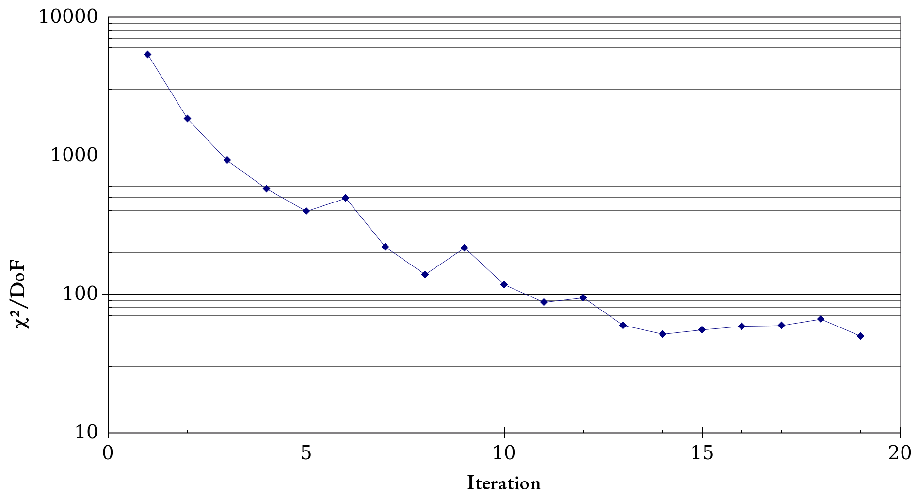
Figure 1: Figure of merit showing the evolution of the $\chi^{2}/DoF$ after each iteration. Iteration 1 corresponds to the initial version of INCL.

For the first study, we chose the very favourable case of the subthreshold proton-induced $K^{+}$ production following the experiment at LINP [14]. This case is very favourable for two reasons. First, the subthreshold $K^{+}$ production is a very specific phenomenon, which involves just a few parameters. Additionally, there is a limited amount of experimental data (70 data points), all coming from the same experimental set up. This highly simplifies both the mandatory analysis of the experimental data (see subsection 3.3) and the analysis of the results. Since all data are from the same experiment, there was no need to rescale the experimental error bars as described in section 4. Second, the experimental data are badly reproduced by INCL [5], which indicates that there is large room for improvement.

On the other hand, this analysis has two limitations. First, the phenomenon studied is a very rare event with cross sections of the order of a few nanobarns. Additionally, each experimental data point corresponds to a different target and different projectile energy, which requires individual calculations. Therefore, it is very CPU intensive to run INCL for this set-up. This forced us to limit the number of experimental data points used in our analysis to 24 representative points. Second, the parameters involved here have an impact on other observables, which are not considered in our analysis. Our approach neglects the possible deterioration of such other observables that might happen when changing the parameters studied here. Therefore, this first study is not physically complete. It will be a proof of concept showing that the approach we developed is functional for complex models like INCL.

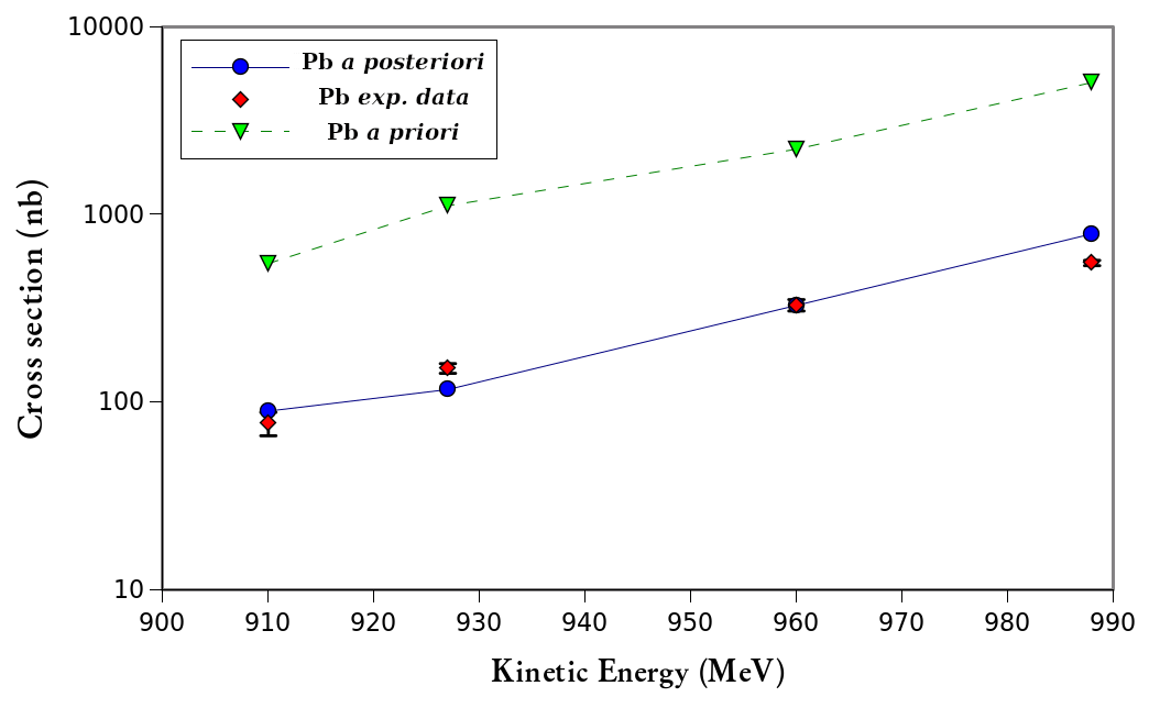
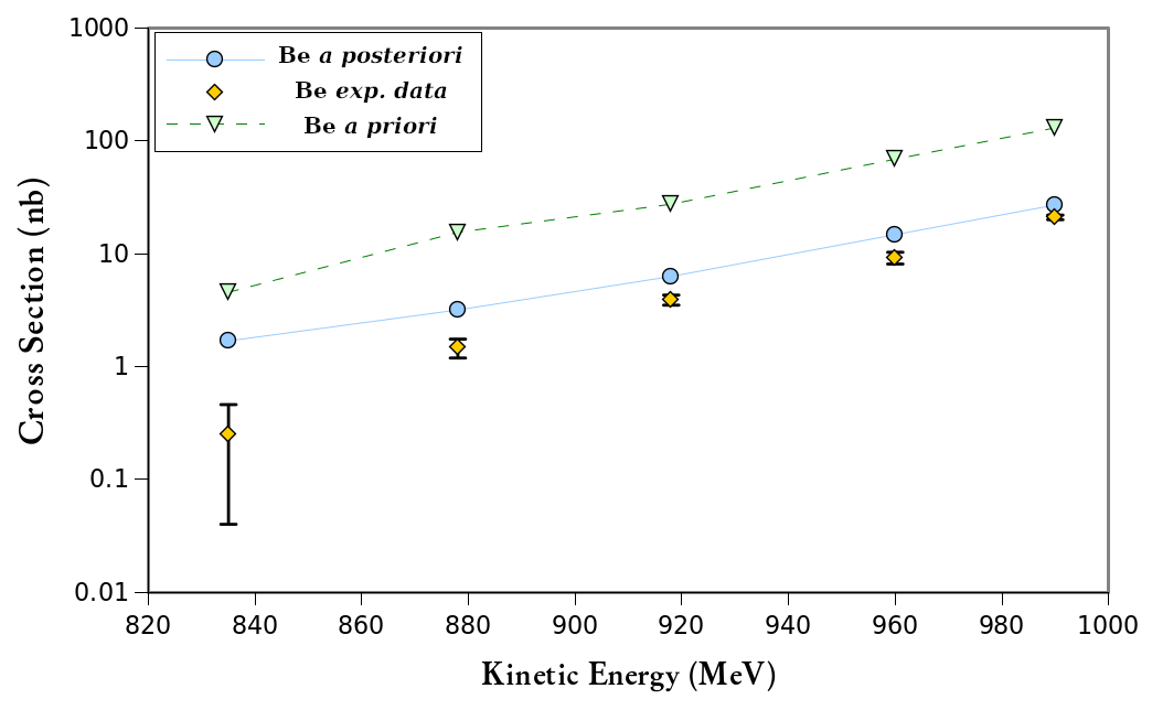
Figure 2: LINP experimental data (Diamonds) [14] compared to INCL before (Triangles)/after (Circles) optimisation for (Top) Lead and (Bottom) Beryllium.

We decided to consider four parameters to be optimised. Namely, the three scalars $a_{NN}$, $a_{\pi N}$, and $a_{\Delta N}$, which are multiplying factors applied to the strangeness production cross sections for $NN$, $\pi N$, and $\Delta N\rightarrow K+X$ reactions, respectively, and a fourth parameter, which is the Fermi momentum used in INCL.

Figure 1 depicts the evolution of the $\chi^{2}/DoF$ after each iteration of the algorithm (see subsection 3.1). Here we only used the Expectation Maximisation due to CPU time restrictions. This calculation took 7 days using 20 cores. Therefore, we will not be able to provide uncertainties for the parameters. After only a few iterations, one can already see a huge improvement of the $\chi^{2}/DoF$ going from more than 5000 to roughly 50. The high initial value of $\sim 5300$ is explained both by the poor initial description of the experimental data (factor 5 in average) and by the rather small experimental error bars (as small as 3%). Regardless of the absolute value of the $\chi^{2}/DoF$, the algorithm succeeds in improving the description of the experimental data by INCL as it is also illustrated in Figure 2. In this figure, one can see that we started from a model highly overestimating the experimental data and we ended with a pretty fair description of the data.

Regarding the parameters, the algorithm multiplied the cross sections for the $NN$, $\pi N$, and $\Delta N\rightarrow K+X$ reactions by factors $1.5$, $0.26$, and $0.43$ respectively and it reduces the Fermi momentum to $232$. Theses values are clearly unphysical and should not be interpreted on physical grounds. However, the study seems to indicate that there is too much energy involved in these type of reactions near the threshold and/or that the cross sections used are overestimated for the lowest energies. Further studies would be necessary to come to a conclusion.

Overall, this example clearly demonstrates the ability of the algorithm to improve the output of a complex model like INCL through the optimisation of its parameters.

5.2 Double differential neutron case

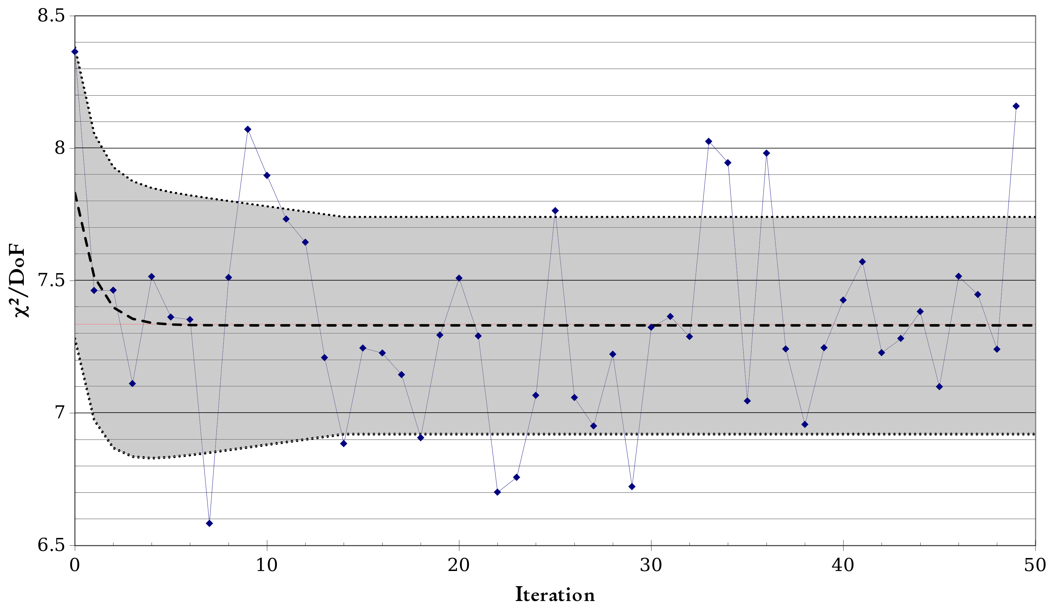
Figure 3: $\chi^{2}/DoF$ of INCL for the DDNXS evaluated for each iteration. The dashed line is a fit of the $\chi^{2}/DoF$ with the shape $a+e^{-bt}$, which is the shape expected from our algorithm. The gray area shows the 1 $\sigma$ standard deviation evaluated for the statistics used in our study.

In a second step, we decided to apply our algorithm to the most important observables for the INCL/ABLA model applications: the double differential neutron cross section (DDNXS). In this case, there are much more parameters relevant for the results than in the previous example. One can mention almost every single elementary double differential cross section (e.g., $NN\rightarrow NN$, $\pi N\rightarrow N\pi\pi$, $\Delta N\rightarrow NN$, etc.), parameters describing the structure of the nucleus, the parameters ruling clustering, the freezing-out temperature in ABLA, etc. Almost everything matters for such a general feature. Here, it is not realistic in terms of CPU power to optimise every single parameter that might be important for the DDNXS. It is therefore necessary to choose the parameters to be optimised. In our case, we have chosen to optimise a parameters scaling the $N\Delta\rightarrow NN$ cross section based on the $NN\rightarrow N\Delta$ cross section (the detailed balance parameter), two parameters for the stopping time of the simulation, and the Fermi momentum. These parameters with enough leeway on their value are supposed to be those with the highest impact on the DDNXS and are therefore the most interesting to study.

Once again, because of CPU time restrictions, we limited the amount of experimental data to be taken into account. Here, we work with the EXFOR data base [15] and we decided to work with proton induced reactions with energies above 200 MeV and for target nuclei lighter than aluminium. This resulted in 7220 experimental data points. As mentioned in subsection 3.3, a careful study of the experimental data used and their possible correlations must be performed in order to obtain/use the best constraints. The most important point in this preliminary study of the experimental data is to make sure that the experimental error bars are consistent. If the error bars are globally over- or underestimated, this will slightly modify the output of the optimisation, notably the error bars of the parameters, and the absolute value of the $\chi^{2}$. However, this problem is of second order compared to the problem introduced by few unrealistically small error bars aside of much more realistic but larger error bars as explained in section 4.

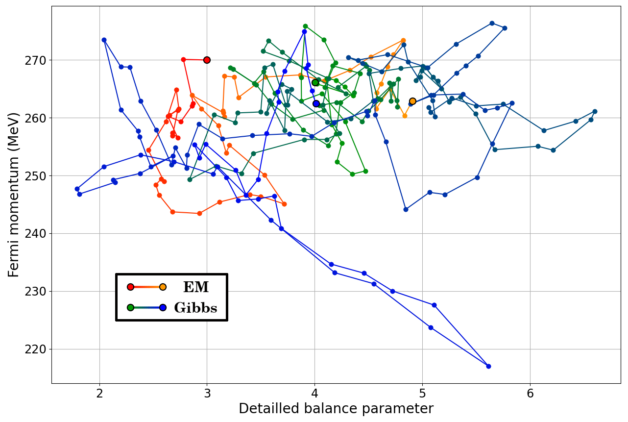
Figure 4: Optimisation of the Fermi momentum and of the detailed balance parameters during the EM (from red to orange) and the Gibbs sampling (from green to blue). The larger bullets indicates the initial and final values for the EM and the Gibbs sampling.

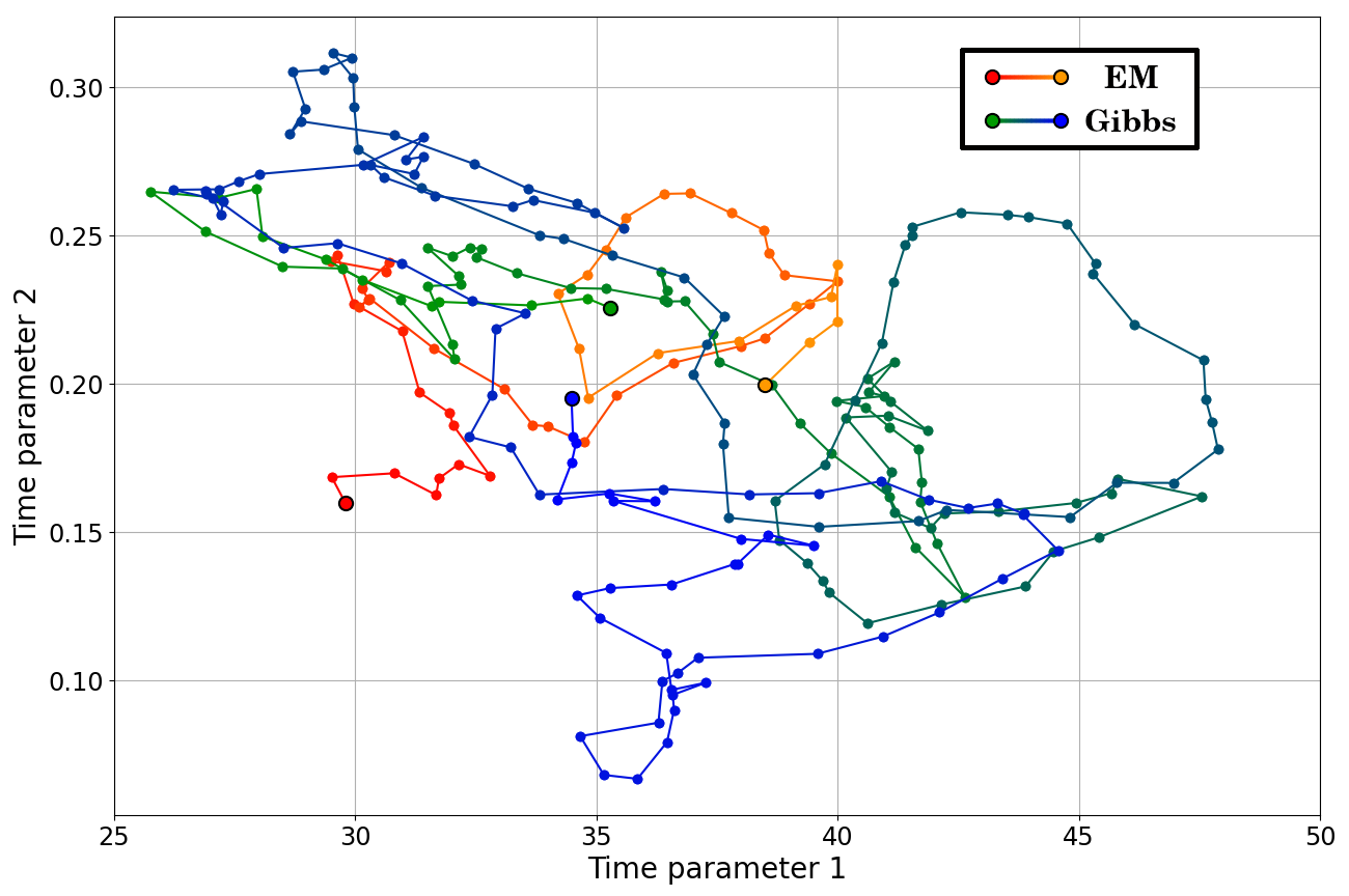
Figure 5: Optimisation of the time parameters during the EM (from red to orange) and the Gibbs sampling (from green to blue). The larger bullets indicates the initial and final values for the EM and the Gibbs sampling.

In the case studied here, there are experimental relative error bars down to 0.12% (EXFOR ID: E2387002, forward neutron emission at 117.5 MeV in the reaction p(137 MeV)+ $C^{Nat}$: $4.31\pm 0.00514$ mb/MeV/sr). This kind of experimental data are toxic for our algorithm because they completely bias the value of the $\chi^{2}$. Therefore, these problematic error bars need to be rescaled. Otherwise, they can also be removed. We selected the first option. Our procedure to rescale experimental error bars is given in section 4. Our approach has not been pushed further as we are first interested in the feasibility of the method.

The execution of our algorithm on the CC-IN2P3 using 20 cores took roughly 60 hours.

First, we evaluated the model quality using the common reduced $\chi^{2}$ throughout the algorithm. Note, the $\chi^{2}/DoF$ plotted in Figure 3 depends on the statistics used. A better statistics reduces the statistical uncertainties and therefore the $\chi^{2}$. Using the standard values for the parameters, the $\chi^{2}/DoF$ is equal to $7.805\pm 0.125$ with a standard deviation of $0.55$. The uncertainty ($\pm 0.125$) of the $\chi^{2}/DoF$ is due to the limited statistics. Using the optimal values as provided by our algorithm, the $\chi^{2}/DoF$ is now $7.34\pm 0.094$ with a standard deviation of $0.41$. This represents an improvement of 6% of the $\chi^{2}/DoF$. The two $\chi^{2}/DoF$ just given have been estimated with the same statistics as in the algorithm to be consistent. Second, the optimal parameters have been evaluated to $4.406\pm 0.131$ (initially $3$) for the detailed balance, $266.4\pm 0.97$ for the Fermi momentum (initially $270$), and for the stopping time parameters to $a=37.13\pm 0.59$ and $b=0.226\pm 0.005$ (initially $a=29.8$ and $b=0.16$). This is illustrated in Figure 4 and Figure 5 by the red/orange dots. The new values indicates that the cross section for the $\Delta$-recombination ($\Delta N\rightarrow NN$) has been increased by $50\%$, the maximal kinetic energy of nucleons has been slightly reduced, and the stopping time has been greatly increased ($t_{stop}=a\times A^{b}$, with $A$ the mass number of the target nucleus). The uncertainties are due to the stochasticity of the model, which is not fully compensated by a high number of iterations in the EM phase of the algorithm. In green/blue, we show the evolution of the parameters along the Gibbs sampling. This provides us the range of parameter values in which the output of the model stays consistent with the experimental data. The a posteriori acceptability range for the parameters are provided by the standard deviation of the multivariate normal distribution obtained. Here, the 1 $\sigma$ acceptability is: $0.986$ (detailed balance), $8.822$ (Fermi momentum), $6.061$ (stopping time parameter 1), $0.0658$ (stopping time parameter 2). Note that the fact the initial and final values obtained are very close is a purely random effect.

These uncertainties can be seen as a domain of validity given the experimental data and the model, which is considered as a valid representation of the truth.

6 Summary and outlook

In this study, we developed an algorithm based on Bayesian statistics able to optimise the parameters of a model using corresponding experimental data. This algorithm is able to fit the model predictions to the experimental data using the optimisation of the free parameters of the model. The objective of this algorithm is twofold: First, the algorithm determines optimal parameters, which minimise the bias of the model and, by extension, the $\chi^{2}$. Second, this algorithm aims at determining the uncertainties of these parameters.

This algorithm has been developed in a global framework, namely the Generalised Least Squares method, which allows an optimisation of the parameters for any model as long as these parameters are allowed to be adjusted.

In our study, we first demonstrated the feasibility of the approach for a selected case, in which we reduced the $\chi^{2}$ of the model by a factor of 100. In a second stage, we studied the neutron double differential cross section with INCL/ABLA in proton-induced reactions on light target nuclei. We were able to produce a reasonable improvement of the model predictions by using thousands of experimental data with a reduction of the $\chi^{2}$ by $6\%$. Despite the fact that the DDNXS are extremely well studied and are already well reproduced by INCL/ABLA, thanks to our algorithm we were still able to slightly improve the model. Even more important, the approach is able to estimate the uncertainties of the model parameters.

We also discussed the limits of the approach with, first, high CPU requirements with several days of calculation with a few tens of cores in the case of INCL. The application of the method will require high performance computing systems in order to reduce the time required for its execution. Another limit of the approach is the availability and the quality of the experimental data. Finally, the disparity of the quality of the experimental data is one of the most important issues, which must be addressed before applying the algorithm. This last point requires to exclude some questionable experimental data with unrealistically small error bars or to rescale these error bars in order to moderate their importance with respect to other data evaluated with a more rigorous approach.

Once the parameters have been optimised, the model bias of the new version of INCL/ABLA can be estimated using the approach developed by Schnabel [4].

Overall, these results are very encouraging showing that Bayesian methods can be used as a tool to improve the description of observables by stochastic nuclear models in the high-energy regime.

7 Acknowledgment

This project has received funding from the Euratom research and training programme 2014-2018 under grant agreement No 847552 (SANDA).

NCCR PlanetS (Swiss National Science Foundation Grant Nr. 51NF40-141881) provided financial support for this research.

Appendix A Derivation of the GLS method

The GLS method is the basis for inference in Bayesian networks of continuous variables with a multivariate normal prior distribution and linear relationships between variables. In this appendix, we will derivate from the Bayes theorem Equation 7 and Equation 9, which form the basis of our algorithm.

Lets assume a set of parameters of interest $\vec{p}$, a model/function $\mathcal{M}$ that we assume to be perfect, and a set of experimental data $\vec{\sigma}_{exp}$. Here, a perfect model stands for $\mathcal{M}(\vec{p}_{true})=\vec{\sigma}_{true}$.

The Bayes theorem gives the relation between the posterior distribution of $\vec{p}$ called $\pi(\vec{p}|\vec{\sigma}_{exp})$, the prior distribution of $\vec{p}$, called $\pi_{0}(\vec{p})$, the prior distribution of $\vec{\sigma}_{exp}$, called $\pi(\vec{\sigma}_{exp})$, and the likelihood of $\vec{\sigma}_{exp}$ knowing $\vec{p}$, called $l(\vec{\sigma}_{exp}|\vec{p})$:

$$\pi(\vec{p}|\vec{\sigma}_{exp})=\frac{l(\vec{\sigma}_{exp}|\vec{p})\times\pi_{0}(\vec{p})}{\pi(\vec{\sigma}_{exp})}.$$ (11)

Here, $\pi(\vec{\sigma}_{exp})$ is a scalar, which guarantees the normalisation of $\pi(\vec{p}|\vec{\sigma}_{exp})$. Both the likelihood $l$ and the prior distribution $\pi_{0}$ are supposed to be multivariate normal distributions. Therefore, we can write:

$$\pi_{0}(\vec{p})\propto\exp\left(-\frac{1}{2}(\vec{p}-\vec{p}_{ref})^{T}\Sigma_{p}^{-1}(\vec{p}-\vec{p}_{ref})\right),$$ (12)

with $\vec{p}_{ref}$ the best a priori estimate of $\vec{p}$ and $\Sigma_{p}$ the covariance matrix of $\vec{p}$, and:

$$l(\vec{\sigma}_{exp}|\vec{p})\propto$$

$$\exp\left(-\frac{1}{2}(\vec{\sigma}_{exp}-\mathcal{M}(\vec{p}))^{T}\Sigma_{e}^{-1}(\vec{\sigma}_{exp}-\mathcal{M}(\vec{p}))\right),$$ (13)

with $\Sigma_{e}$ the covariance matrix of $\vec{\sigma}$ and $\mathcal{M}$ the assumed to be perfect model.

Since the product of two (multivariate) normal distributions is also a (multivariate) normal distribution, we also have:

$$\pi(\vec{p}|\vec{\sigma}_{exp})\propto\exp\left(-\frac{1}{2}(\vec{p}-\vec{p}_{op})^{T}\Sigma_{op}^{-1}(\vec{p}-\vec{p}_{op})\right),$$ (14)

with $\vec{p}_{op}$ and $\Sigma_{op}$ the optimal parameter set for the model, knowing the experimental data set $\vec{\sigma}_{exp}$, and the corresponding covariance matrix, respectively.

Since the GLS method requires linear relationships between variables, we need to approximate the model $\mathcal{M}$ with a Taylor series approximation:

$$\mathcal{M}(\vec{p})=\mathcal{M}(\vec{p}_{ref})+J_{p}(\vec{p}-\vec{p}_{ref}),$$ (15)

with $J_{p}$ the Jacobian of the model.

Therefore, we can rewrite the likelihood as:

$$l(\vec{\sigma}_{exp}|\vec{p})\propto$$

$$\exp\left(-\frac{1}{2}(\vec{\sigma}_{exp}-\mathcal{M}(\vec{p}_{ref})-J_{p}(\vec{p}-\vec{p}_{ref}))^{T}\Sigma_{e}^{-1}\right.$$

$$\qquad\left.{\color[rgb]{1,1,1}\frac{1}{2}}(\vec{\sigma}_{exp}-\mathcal{M}(\vec{p}_{ref})-J_{p}(\vec{p}-\vec{p}_{ref}))\right),$$ (16)

which can be simplified as:

$$l(\vec{\sigma}_{exp} |\vec{p})\propto$$

$$\exp\left(-\frac{1}{2}(H_{ref}-J_{p}\vec{p})^{T}\Sigma_{e}^{-1}(H_{ref}-J_{p}\vec{p})\right).$$ (17)

with the substitution of the constant term $H_{ref}~{}=~{}\vec{\sigma}_{exp}-\mathcal{M}(\vec{p}_{ref})+J_{p}\vec{p}_{ref}$.

With a combination of equations 11, 12, 14, and A, and knowing that $\pi(\vec{\sigma}_{exp})$ is a scalar, we have:

$$\exp \left(-\frac{1}{2}(\vec{p}-\vec{p}_{op})^{T}\Sigma_{op}^{-1}(\vec{p}-\vec{p}_{op})\right)\propto$$

$$\exp\left(-\frac{1}{2}(\vec{p}-\vec{p}_{ref})^{T}\Sigma_{p}^{-1}(\vec{p}-\vec{p}_{ref})\right)\times$$

$$\exp\left(-\frac{1}{2}(H_{ref}-J_{p}\vec{p})^{T}\Sigma_{e}^{-1}(H_{ref}-J_{p}\vec{p})\right)$$ (18)

With this, it follows:

$$(\vec{p}- \vec{p}_{op})^{T}\Sigma_{op}^{-1}(\vec{p}-\vec{p}_{op})+C=$$

$$(\vec{p}-\vec{p}_{ref})^{T}\Sigma_{p}^{-1}(\vec{p}-\vec{p}_{ref})+$$

$$(H_{ref}-J_{p}\vec{p})^{T}\Sigma_{e}^{-1}(H_{ref}-J_{p}\vec{p}),$$ (19)

with $C$ a constant of normalisation.

Since $\vec{p}$ is the only variable in Appendix A, the coefficients must match for the terms with $(\vec{p})^{T}$ on the left hand side and those with $\vec{p}$ on the right hand side. We then have the four equations:

$$\Sigma_{op}^{-1} =\Sigma_{p}^{-1}+J_{p}^{T}\Sigma_{e}^{-1}J_{p}$$ (20)

$$\Sigma_{op}^{-1}\vec{p}_{op} =\Sigma_{p}^{-1}\vec{p}_{ref}+J_{p}^{T}\Sigma_{e}^{-1}H_{ref}$$ (21)

$$(\vec{p}_{op})^{T}\Sigma_{op}^{-1} =(\vec{p}_{ref})^{T}\Sigma_{p}^{-1}+H_{ref}^{T}\Sigma_{e}^{-1}J_{p}$$ (22)

$$(\vec{p}_{op})^{T}\Sigma_{op}^{-1} \vec{p}_{op}+C=$$

$$(\vec{p} {}_{ref})^{T}\Sigma_{p}^{-1}\vec{p}_{ref}+H_{ref}^{T}\Sigma_{e}^{-1}H_{ref}$$ (23)

Using the Woodbury matrix identity in Equation 20, we have:

$$\Sigma_{op}=\Sigma_{p}-\Sigma_{p}J_{p}^{T}(\Sigma_{e}+J_{p}\Sigma_{p}J_{p}^{T})^{-1}J_{p}\Sigma_{p}$$ (24)

Multiplying Equation 21 from the left with Equation 24, we get:

$$\vec{p}_{op} =\left(\Sigma_{p}-\Sigma_{p}J_{p}^{T}(\Sigma_{e}+J_{p}\Sigma_{p}J_{p}^{T})^{-1}J_{p}\Sigma_{p}\right)\left(\Sigma_{p}^{-1}\vec{p}_{ref}+J_{p}^{T}\Sigma_{e}^{-1}H_{ref}\right)$$

$$=\vec{p}_{ref}+\Sigma_{p}J_{p}^{T}\Sigma_{e}^{-1}H_{ref}-\Sigma_{p}J_{p}^{T}(\Sigma_{e}+J_{p}\Sigma_{p}J_{p}^{T})^{-1}J_{p}\vec{p}_{ref}$$

$$\qquad\qquad\qquad\qquad\qquad\qquad\qquad\qquad\qquad\qquad\qquad-\Sigma_{p}J_{p}^{T}(\Sigma_{e}+J_{p}\Sigma_{p}J_{p}^{T})^{-1}J_{p}\Sigma_{p}J_{p}^{T}\Sigma_{e}^{-1}H_{ref}$$

$$=\vec{p}_{ref}-\Sigma_{p}J_{p}^{T}(\Sigma_{e}+J_{p}\Sigma_{p}J_{p}^{T})^{-1}J_{p}\vec{p}_{ref}+\Sigma_{p}J_{p}^{T}\left(\Sigma_{e}^{-1}-(\Sigma_{e}+J_{p}\Sigma_{p}J_{p}^{T})^{-1}J_{p}\Sigma_{p}J_{p}^{T}\Sigma_{e}^{-1}\right)H_{ref}$$

$$=\vec{p}_{ref}-\Sigma_{p}J_{p}^{T}(\Sigma_{e}+J_{p}\Sigma_{p}J_{p}^{T})^{-1}J_{p}\vec{p}_{ref}$$

$$\qquad\qquad\qquad\qquad\qquad+\Sigma_{p}J_{p}^{T}(\Sigma_{e}+J_{p}\Sigma_{p}J_{p}^{T})^{-1}\left((\Sigma_{e}+J_{p}\Sigma_{p}J_{p}^{T})\Sigma_{e}^{-1}-J_{p}\Sigma_{p}J_{p}^{T}\Sigma_{e}^{-1}\right)H_{ref}$$

$$=\vec{p}_{ref}-\Sigma_{p}J_{p}^{T}(\Sigma_{e}+J_{p}\Sigma_{p}J_{p}^{T})^{-1}J_{p}\vec{p}_{ref}+\Sigma_{p}J_{p}^{T}(\Sigma_{e}+J_{p}\Sigma_{p}J_{p}^{T})^{-1}H_{ref}$$

$$=\vec{p}_{ref}+\Sigma_{p}J_{p}^{T}(\Sigma_{e}+J_{p}\Sigma_{p}J_{p}^{T})^{-1}(H_{ref}-J_{p}\vec{p}_{ref})$$ (25)

and, replacing $H_{ref}$, we finally obtain:

$$\vec{p}_{op} =\vec{p}_{ref}+$$

$$\Sigma_{p}J_{p}^{T}(\Sigma_{e}+J_{p}\Sigma_{p}J_{p}^{T})^{-1}(\vec{\sigma}_{exp}-\mathcal{M}(\vec{p}_{ref}))$$ (26)

It is important to emphasise that equation Appendix A is only valid as long as the hypothesis of a linear model is valid. However, most realistic models can be approximated by a linear model only locally. Therefore, $\mathcal{M}(\vec{p}_{ref})$ must be estimated reversing Equation 15:

$$\mathcal{M}_{lin}(\vec{p}_{ref})=\mathcal{M}(\vec{p})+J_{p}(\vec{p}_{ref}-\vec{p}),$$ (27)

with $J_{p}$ the Jacobian of the model in $\vec{p}$.

In order to simplify Appendix A, we usually introduce the matrix of regression $\tilde{\Sigma}_{i}$ defined using Equation 5. Explicitly, the equation expands as:

$$\tilde{\Sigma}_{i}=J_{i}\ \Sigma\ J_{i}^{T} =\left(\begin{matrix}\Sigma_{e}+J_{p}\Sigma_{p}J_{p}^{T}&J_{p}\Sigma_{p}\\ \Sigma_{p}J_{p}^{T}&\Sigma_{p}\\ \end{matrix}\right)$$

$$=\left(\begin{matrix}\tilde{\Sigma}_{DD_{i}}&\tilde{\Sigma}_{DI_{i}}\\ \tilde{\Sigma}_{ID_{i}}&\tilde{\Sigma}_{II_{i}}\\ \end{matrix}\right).$$ (28)

We finally obtain Equation 7:

$$\vec{p}_{op}=\vec{p}_{ref}+\tilde{\Sigma}_{ID_{i}}\left(\tilde{\Sigma}_{DD_{i}}\right)^{-1}\left[\vec{\sigma}_{exp}-\mathcal{M}_{lin}(\vec{p}_{ref})\right],$$ (29)

and Equation 9 follows from Equation 24:

$$\Sigma_{op}=\tilde{\Sigma}_{II_{i}}-\tilde{\Sigma}_{ID_{i}}\left(\tilde{\Sigma}_{DD_{i}}\right)^{-1}\tilde{\Sigma}_{DI_{i}}.$$ (30)

As the difference $|\vec{p}_{op}-\vec{p}|$ becomes smaller, the hypothesis of a linear model between $\vec{p}$ and $\vec{p}_{op}$ becomes more applicable, and therefore, the last two equations become more exact. This justifies the use of an iterative algorithm evaluating a linearisation of the model (Equation 2 : $\vec{T_{i}}$) and its Jacobian (Equation 4 : $J_{p_{i}}$) in $\vec{p}_{i}$, the best evaluation of the optimal parameters currently known and then, evaluating an improved $\vec{p}_{i+1}$ from $\vec{T_{i}}$ and $J_{p_{i}}$ using Equation 7.

References

- [1] Myrrha project. Website.
- [2] European commission: Chanda. Website.
- [3] European commission: Sanda. Website.
- [4] G. Schnabel et al. Report on the development of methodology for the uncertainty quantification of (not only) high-energy models. Report D11.6 within the CHANDA European project FP7-Fission-2013-605203, 2018.
- [5] J. Hirtz et al. Strangeness production in the new version of the liège intra-nuclear cascade model. Phys. Rev. C, 101:014608, 2020.
- [6] J. L. Rodríguez-Sánchez et al. Hypernuclei formation in spallation reactions by coupling the liège intranuclear cascade model to the deexcitation code abla. Phys. Rev. C, 105:014623, 2022.
- [7] J. L. Rodríguez-Sánchez et al. Constraint of the nuclear dissipation coefficient in fission of hypernuclei. Phys. Rev. Lett., 130:132501, 2023.
- [8] G. Schnabel. Estimating model bias over the complete nuclide chart with sparse gaussian processes at the example of incl/abla and double-differential neutron spectra. EPJ Nuclear Sci. Technol., 4:33, 2018.
- [9] R. Hanson C. Lawson. Solving Least Squares Problems. Prentice-Hall, Englewood Cliffs, NJ, 1974.
- [10] D. Rubin A. Dempster, N. Laird. Maximum likelihood from incomplete data via the em algorithm. Journal of the Royal Statistical Society, Series B., 39(1):1–38, 1977.
- [11] G. Schnabel. Fitting and analysis technique for inconsistent nuclear data.
- [12] D. Neudecker et al. Applying a template of expected uncertainties to updating 239pu(n,f) cross-section covariances in the neutron data standards database. Nuclear Data Sheets, 163:228–248, 2020.
- [13] P. Helgesson et al. Combining total monte carlo and unified monte carlo: Bayesian nuclear data uncertainty quantification from auto-generated experimental covariances. Progress in Nuclear Energy, 96:76–96, 2017.
- [14] V. Koptev et al. Subthreshold -meson production in proton-nucleus interactions. Zh. Eksp. Teor. Fiz., 94:1–14, 1988.
- [15] V.V. Zerkin and B. Pritychenko. The experimental nuclear reaction data (exfor): Extended computer database and web retrieval system. NIM A, 888:31, 2018.