Strange hidden-charm pentaquark poles from $B^{-}\to J/\psi\Lambda\bar{p}$

Abstract

Recent LHCb data for $B^{-}\to J/\psi\Lambda\bar{p}$ show a clear peak structure at the $\Xi_{c}\bar{D}$ threshold in the $J/\psi\Lambda$ invariant mass ($M_{J/\psi\Lambda}$) distribution. The LHCb’s amplitude analysis identified the peak with the first hidden-charm pentaquark with strangeness $P_{\psi s}^{\Lambda}(4338)$. We conduct a coupled-channel amplitude analysis of the LHCb data by simultaneously fitting the $M_{J/\psi\Lambda}$, $M_{J/\psi\bar{p}}$, $M_{\Lambda\bar{p}}$, and $\cos\theta_{K^{*}}$ distributions. Rather than the Breit-Wigner fit employed in the LHCb analysis, we consider relevant threshold effects and a unitary $\Xi_{c}\bar{D}$-$\Lambda_{c}\bar{D}_{s}$ coupled-channel scattering amplitude from which $P_{\psi s}^{\Lambda}$ poles are extracted for the first time. In our default fit, the $P_{\psi s}^{\Lambda}(4338)$ pole is almost a $\Xi_{c}\bar{D}$ bound state at $(4338.2\pm 1.4)-(1.9\pm 0.5)\,i$ MeV. Our default model also fits a large fluctuation at the $\Lambda_{c}\bar{D}_{s}$ threshold, giving a $\Lambda_{c}\bar{D}_{s}$ virtual state, $P_{\psi s}^{\Lambda}(4255)$, at $4254.7\pm 0.4$ MeV. We also found that the $P_{\psi s}^{\Lambda}(4338)$ peak cannot solely be a kinematical effect, and a nearby pole is needed.

1 Introduction

The first discovery of a strange hidden-charm pentaquark $P_{\psi s}^{\Lambda}(4338)$ in $B^{-}\to J/\psi\Lambda\bar{p}$ was recently reported by the LHCb Collaboration lhcb_seminar . The data shows a clear peak in the $J/\psi\Lambda$ invariant mass ($M_{J/\psi\Lambda}$) distribution, suggesting the pentaquark contribution. The LHCb conducted an amplitude analysis to determine the pentaquark mass, width, and spin-parity to be $4338.2\pm 0.7\leavevmode\nobreak\ {\rm MeV}$, $7.0\pm 1.2\leavevmode\nobreak\ {\rm MeV}$, and $J^{P}=1/2^{-}$, respectively. These resonance parameters are primary basis to address the nature and internal structure of $P_{\psi s}^{\Lambda}(4338)$. Our concern here is that the LHCb analysis assumed that the resonance-like peak can be well described with a Breit-Wigner (BW) amplitude. Actually, the resonance peak sits right on the $\Xi_{c}\bar{D}$ threshold [see Fig. 2(a)]. The BW fit is often unsuitable in this situation because a kinematical effect (threshold cusp) may cause the resonancelike structure. Even if there exists a relevant pole that couples with the $\Xi_{c}\bar{D}$ channel, the branch cut from the $\Xi_{c}\bar{D}$ channel would distort the lineshape due to the pole, invalidating the BW fit.

Thus, in this work, we conduct a coupled-channel amplitude analysis of the LHCb data on $B^{-}\to J/\psi\Lambda\bar{p}$ with all relevant kinematical effects taken into account; see Ref. ours for details. We fit our amplitude model to the $M_{J/\psi\Lambda}$, $M_{J/\psi\bar{p}}$, $M_{\Lambda\bar{p}}$, and $\cos\theta_{K^{*}}$ distribution data simultaneously. Our model does not include BW amplitudes but a unitary $\Xi_{c}\bar{D}$-$\Lambda_{c}\bar{D}_{s}$ coupled-channel amplitude with which we address whether the LHCb data requires pentaquark poles.

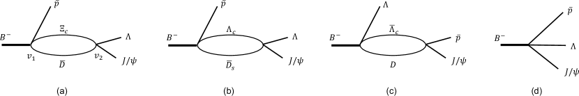
Figure 1: $B^{-}\to J/\psi\Lambda\bar{p}$ mechanisms considered in this work. The diagrams (a)-(d) have different weak vertices $v_{1}$ such as (a) $B^{-}\to\Xi_{c}\bar{D}\bar{p}$, (b) $B^{-}\to\Lambda_{c}\bar{D}_{s}\bar{p}$, (c) $B^{-}\to\bar{\Lambda}_{c}D\Lambda$, and (d) $B^{-}\to J/\psi\Lambda\bar{p}$. The vertex $v_{2}$ in (a,b) is a $\Xi_{c}\bar{D}-\Lambda_{c}\bar{D}_{s}$ coupled-channel scattering and a perturbative transition to $J/\psi\Lambda$ while, in (c), an elastic $\bar{\Lambda}_{c}D$ scattering and a perturbative transition to $J/\psi\bar{p}$. Figures taken from Ref. ours . Copyright (2023) APS.

2 Model

In the invariant mass distributions of $B^{-}\to J/\psi\Lambda\bar{p}$, noticeable structures can be seen at the $\Xi_{c}\bar{D}$, $\Lambda_{c}\bar{D}_{s}$, and $\bar{\Lambda}_{c}D$ thresholds. This suggests that threshold cusps from the diagrams in Figs. 1(a-c) cause the structures; hadronic rescatterings and the associated poles could further enhance or suppress the cusps. Thus our amplitude model considers the diagrams of Figs. 1(a-c), and also a direct decay of Fig. 1(d) that would absorb other possible mechanisms. We consider only $s$-wave interactions that are expected to be dominant since the $Q$-value is not so large ($\sim 130$ MeV).

We include the most important coupled-channels in the hadronic scatterings; a $\Xi_{c}\bar{D}-\Lambda_{c}\bar{D}_{s}(1/2^{-})$ coupled-channel in Figs. 1(a,b), and a $\bar{\Lambda}_{c}D(1/2^{+})$ single-channel in Fig. 1(c). Our data-driven approach employs contact separable hadron interactions not biased by any particular models, and determine all coupling strengths by fitting the data. The relevant coupled-channel unitarity is respected. These scatterings are followed by perturbative transitions to the final $J/\psi\Lambda$ and $J/\psi\bar{p}$ states in our model.

3 Results

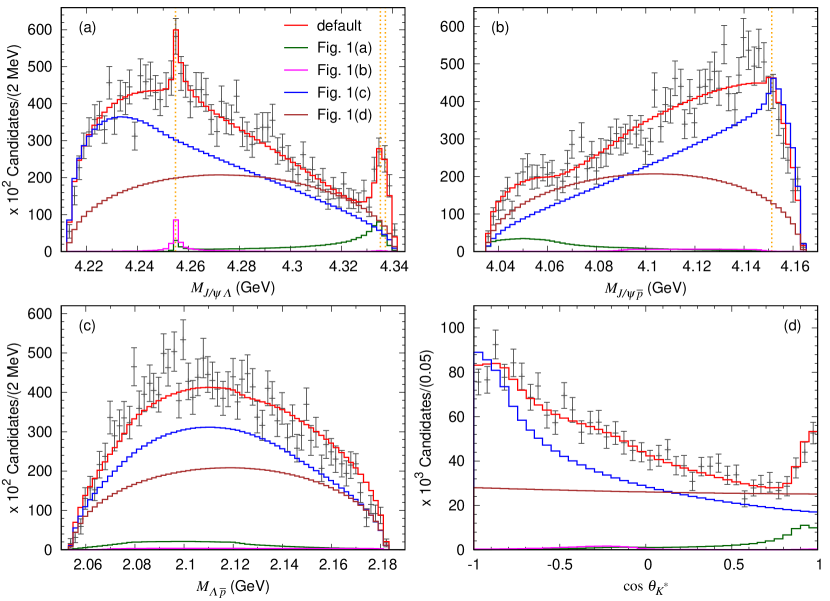
Figure 2: Simultaneous fit to (a) $J/\psi\Lambda$, (b) $J/\psi\bar{p}$, (c) $\Lambda\bar{p}$ invariant mass, and (d) $\cos\theta_{K^{*}}$ distributions of $B^{-}\to J/\psi\Lambda\bar{p}$ from the LHCb lhcb_seminar ; efficiency-corrected and background-subtracted data. The plots are the default fit and each contribution from diagrams in Fig. 1. The dotted vertical lines in the panel (a) [(b)] indicate $\Lambda_{c}^{+}D_{s}^{-}$, $\Xi_{c}^{0}\bar{D}^{0}$, and $\Xi_{c}^{+}D^{-}$ [$\bar{\Lambda}_{c}^{-}D^{0}$] thresholds from left to right. Figures taken from Ref. ours . Copyright (2023) APS.

The $M_{J/\psi\Lambda}$, $M_{J/\psi\bar{p}}$, $M_{\Lambda\bar{p}}$, and $\cos\theta_{K^{*}}$ distributions from the LHCb are simultaneously fitted with our model described in the previous section; $\cos\theta_{K^{*}}\equiv\bm{p}_{\Lambda}\cdot\bm{p}_{\psi}/|\bm{p}_{\Lambda}||\bm{p}_{\psi}|$ in the $\Lambda\bar{p}$ center-of-mass frame. In our default fit, we adjust 9 fitting parameters from coupling strengths of the weak vertices and hadronic interactions. The fit result is shown in Fig. 2; $\chi^{2}/{\rm ndf}\simeq 1.21$ with ’ndf’ being the number of bins minus the number of the fitting parameters. The presented binned theoretical distributions are obtained by smearing theoretical invariant mass ($\cos\theta_{K^{*}}$) distributions with experimental resolutions of 1 MeV (bin width of 0.05), and then averaging them over the bin width in each bin. The LHCb data, including the $P_{\psi s}^{\Lambda}(4338)$ peak at $M_{J/\psi\Lambda}\sim 4338$ MeV, are well fitted by our default model as seen in Fig. 2. Our default model also fits a large fluctuation at $M_{J/\psi\Lambda}\sim 4255$ MeV. The LHCb analysis concluded this fluctuation to be a statistical one. However, considering the fact that the fluctuation sits just right on the $\Lambda_{c}\bar{D}_{s}$ threshold, we can expect a visible threshold cusp from a color-favored $B^{-}\to\Lambda_{c}\bar{D}_{s}\bar{p}$ followed by $\Lambda_{c}\bar{D}_{s}\to J/\psi\Lambda$. The cusp might have been enhanced by a $\Lambda_{c}\bar{D}_{s}$ rescattering and an associated $P_{\psi s}^{\Lambda}(4255)$ pole.

Each Contribution from the diagrams in Fig. 1 is also given in Fig. 2. Dominant mechanisms are Figs. 1(c) [blue] and 1(d) [brown]. We can understand that the increasing $M_{J/\psi\bar{p}}$ distribution in Fig. 2(b) is from Fig. 1(c) that causes the $\bar{\Lambda}_{c}D$ threshold cusp. Our fit found that the cusp is suppressed by a repulsive $\bar{\Lambda}_{c}D$ interaction, which is consistent with our previous analysis of $B^{0}_{s}\to J/\psi p\bar{p}$ sxn_Bs . Contributions from the diagrams of Figs. 1(a) [green] and 1(b) [magenta] are smaller in the magnitude. However, they show significantly enhanced $\Xi_{c}\bar{D}$ and $\Lambda_{c}\bar{D}_{s}$ threshold cusps. The $P_{\psi s}^{\Lambda}$ peaks are caused by them through the interference.

There are qualitative differences between our and LHCb’s descriptions of the data. In the LHCb analysis, the $M_{J/\psi\bar{p}}$ distribution is fitted with a non-resonant $p$-wave $J/\psi\bar{p}$ [NR($J/\psi\bar{p}$)] amplitude in a polynomial form, and the physical origin of the increasing behavior is not clarified. The NR($J/\psi\bar{p}$) contribution reaches $\sim 84$% fit fraction. Since a $s$-wave dominance is usually expected in the small $Q$-value process, this $p$-wave dominance is difficult to understand. Our model includes $s$-wave $J/\psi\bar{p}$ only. Regarding the number of fitting parameters, 16 in the LHCb’s model while 9(8) in our default (alternative) model. Since the LHCb fitted richer information from six-dimensional data, they would need more parameters. However, this might not fully explain $\sim 2$ times more parameters. Rather, we suspect that the $p$-wave dominance and excessive parameters are due to missing relevant mechanisms such as Figs. 1(a-c), since many other mechanisms would be needed to mimic the relevant ones through complicated interferences.

Our default $\Xi_{c}\bar{D}-\Lambda_{c}\bar{D}_{s}(1/2^{-})$ coupled-channel scattering amplitude is analytically continued to find relevant poles. We found $P_{\psi s}^{\Lambda}(4338)$ pole at $(4338.2\pm 1.4)-(1.9\pm 0.5)\,i$ MeV; $J^{P}=1/2^{-}$ is consistent with the LHCb result. We also found $P_{\psi s}^{\Lambda}(4255)$ pole at $4254.7\pm 0.4$ MeV. Figure 3 illustrates where the poles are located relative to the relevant thresholds. As seen in the figure, the $P_{\psi s}^{\Lambda}(4338)$ pole is a $\Xi_{c}\bar{D}$ bound state slightly shifted due to a coupled-channel effect. Also, the $P_{\psi s}^{\Lambda}(4255)$ pole is essentially a $\Lambda_{c}\bar{D}_{s}$ virtual state.

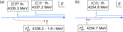
Figure 3: (a)[(b)] $P_{\psi s}^{\Lambda}(4338)$ [$P_{\psi s}^{\Lambda}(4255)$] pole position from the default model. The branch cuts are indicated by the double lines. The red dotted arrows connect the poles and their closest physical energy regions. Figures taken from Ref. ours . Copyright (2023) APS.

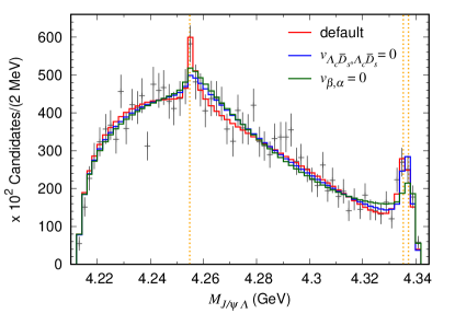
Figure 4: Default and alternative fits to the LHCb data for $B^{-}\to J/\psi\Lambda\bar{p}$ lhcb_seminar . Figures taken from Ref. ours . Copyright (2023) APS.

We also considered alternative models without $P_{\psi s}^{\Lambda}(4255)$ pole, and with/without energy dependence in $\Xi_{c}\bar{D}$ interaction. We obtained comparable fits as shown in Fig. 4[blue]. There is still a $\Lambda_{c}\bar{D}_{s}$ threshold cusp without a nearby pole. The default and alternative models have $P_{\psi s}^{\Lambda}(4338)$ poles on different Riemann sheets, suggesting the need of more precise data for $B^{-}\to\Lambda_{c}\bar{D}_{s}\bar{p}$ and also $\Xi^{-}_{b}\to J/\psi\Lambda K^{-}$. We also examined if the $\Xi_{c}\bar{D}$ threshold cusp without a nearby pole can explain the $P_{\psi s}^{\Lambda}(4338)$ peak, as shown in Fig. 4 [green]. We find a noticeably worse fit in the $P_{\psi s}^{\Lambda}(4338)$ region, concluding that a nearby pole is needed to enhance the cusp.

Acknowledgments
This work is in part supported by National Natural Science Foundation of China (NSFC) under contracts U2032103 (S.X.N.) and under Grants No. 12175239 and 12221005 (J.J.W.).

References

- (1) R. Aaij et al. (LHCb Collaboration), Phys. Rev. Lett. 131, 031901 (2023).
- (2) S.X. Nakamura and J.-J. Wu, Phys. Rev. D 108, L011501 (2023).
- (3) S.X. Nakamura, A. Hosaka, and Y. Yamaguchi, Phys. Rev. D 104, L091503 (2021).