Cut-and-paste for impulsive gravitational waves with $\Lambda$:
The mathematical analysis

Abstract

Impulsive gravitational waves are theoretical models of short but violent bursts of gravitational radiation. They are commonly described by two distinct spacetime metrics, one of local Lipschitz regularity, the other one even distributional. These two metrics are thought to be ‘physically equivalent’ since they can be formally related by a ‘discontinuous coordinate transformation’. In this paper we provide a mathematical analysis of this issue for the entire class of nonexpanding impulsive gravitational waves propagating in a background spacetime of constant curvature. We devise a natural geometric regularisation procedure to show that the notorious change of variables arises as the distributional limit of a family of smooth coordinate transformations. In other words, we establish that both spacetimes arise as distributional limits of a smooth sandwich wave taken in different coordinate systems which are diffeomorphically related.

Keywords: impulsive gravitational waves, nonlinear distributional geometry, discontinuous coordinate transformation.

MSC2010: 83C15, 83C35, 46F30, 83C10, 34A36

PACS numbers: 04.20.Jb, 02.30.Hq,

1 Introduction

Impulsive gravitational waves are exact general relativistic spacetimes providing theoretic models of short but strong bursts of gravitational radiation. Originally introduced by R. Penrose (e.g. [31]) they have since attracted the attention of researchers in exact spacetimes (who have widely generalised the original class of solutions, see e.g. [33]), of theoretical physicists (who have considered quantum scattering and the memory effect in these geometries as well as their astrophysical applications, see e.g. [46, 4]), and of mathematicians (who have used them as relevant key-models in low regularity Lorentzian geometry). For a pedagogical introduction of the various constructions and models as well as their physical properties see [15, Chapter 20].

Here we focus on a fundamental mathematical issue related to the fact that impulsive gravitational waves are metrics of low regularity. Indeed, they are commonly described by two ‘forms’ of the metric, one (locally Lipschitz-)continuous, the other one distributional. The ‘physical equivalence’ of these two descriptions has been established in several families of these models in a formal way, leaving open some quite subtle problems in low regularity Lorentzian geometry. In fact, both ‘forms’ of the metric are connected via a ‘discontinuous coordinate transformation’ which reflects the Penrose junction conditions used to vividly construct these spacetimes in the first place. This ‘scissors and paste’ approach [31] was recently generalised to the $\Lambda\not=0$-case [39].

In this work we completely solve these mathematical issues for the class of all nonexpanding impulsive gravitational waves propagating on backgrounds of constant curvature, i.e., Minkowski space and the (anti-)de Sitter universe. We do so by employing nonlinear distributional geometry, a method which is based on regularisation of the rough metrics and which also brings to light new insights into the geometry and the physics of these spacetimes. We build upon the (nonlinear) distributional analysis of the geodesics in these spacetimes carried out in [45] and [43]. Thereby the current work concludes this long term research effort in a completely satisfactory way.

This article is organised in the following way. In the next section we recall the relevant aspects of the class of solutions we are working with. In particular, we discuss explicitly the ‘discontinuous coordinate transformation’ thereby also fixing our notations and conventions. We also outline how our results and methods are related to previous works in the case $\Lambda=0$ [20]. Then, in Section 3, we collect the necessary results from the nonlinear distributional analysis of the geodesics in the class of solutions at hand and fix our notation concerning nonlinear distributional geometry. Next, in Section 4 we study a special class of null geodesics, namely the null generators of (anti-)de Sitter space in a $5$-dimensional flat space with impulsive wave which provides us with a natural geometric regularisation of the notorious transformation. In Section 5 we analyse the regularised transformation and show that it is a generalised diffeomorphism in the sense of nonlinear distributional geometry. We close with a discussion of our results in Section 6.

2 Nonexpanding impulsive waves with $\Lambda$

Here we describe the class of nonexpanding impulsive waves with an arbitrary value of $\Lambda$. These geometries have come into focus with the landmark work of Hotta and Tanaka [19], where in analogy with the classical Aichelburg-Sexl approach [3], the Schwarzschild–(anti-)de Sitter solution is boosted to ultrarelativistic speed to obtain a nonexpanding impulsive gravitational wave generated by a pair of null monopole particles. For an overview of the many more such solutions that have been found since, see e.g. [37, Section 2].

2.1 Metric representations & the ‘discontinuous transformation’

In conformally flat coordinates these solutions for any value of $\Lambda$ take the distributional form [35]

$${\rm{d}}s^{2}=\frac{2\,{\rm{d}}\eta\,{\rm{d}}\bar{\eta}-2\,{\rm{d}}{\mathcal{U}}\,{\rm{d}}{\mathcal{V}}+2{\mathcal{H}}(\eta,\bar{\eta})\,\delta({{\mathcal{U}}})\,{\rm{d}}{{\mathcal{U}}}^{2}}{[\,1+\frac{1}{6}\Lambda(\eta\bar{\eta}-{{\mathcal{U}}}{{\mathcal{V}}})\,]^{2}}\,,$$ (2.1)

where ${\mathcal{H}}$ is a real-valued function and $\delta$ is the Dirac-distribution. Due to the occurrence of a distributional coefficient, (2.1) lies far beyond the Geroch-Traschen class of metrics [12], which is defined by possessing Sobolev regularity $W^{1,2}_{\mbox{\small loc}}\cap L^{\infty}_{\mbox{\small loc}}$. It is known to be the largest class which allows in general to stably define the curvature in distributions (see also [27, 50]). Nevertheless, due to its simple structure the curvature of (2.1) can be computed explicitly to give the impulsive Newman-Penrose components $\Psi_{4}=(1+\frac{1}{6}\Lambda\eta\bar{\eta})^{2}{\mathcal{H}}_{,\eta\eta}\delta({{\mathcal{U}}})$, and $\Phi_{22}=(1+\frac{1}{6}\Lambda\eta\bar{\eta})\big{(}(1+\frac{1}{6}\Lambda\eta\bar{\eta}){\mathcal{H}}_{,\eta\bar{\eta}}+\frac{1}{6}\Lambda({\mathcal{H}}-\eta{\mathcal{H}}_{,\eta}-\bar{\eta}{\mathcal{H}}_{,\bar{\eta}})\big{)}\delta({{\mathcal{U}}})$.

The corresponding continuous form of the metric is given by [32, 35]

$${\rm{d}}s^{2}=\frac{2\,|{\rm{d}}Z+u_{+}(h_{,Z\bar{Z}}{\rm{d}}Z+{h}_{,\bar{Z}\bar{Z}}{\rm{d}}\bar{Z})|^{2}-2\,{\rm{d}}u{\rm{d}}v}{[\,1+\frac{1}{6}\Lambda(Z\bar{Z}-uv+u_{+}G)\,]^{2}}\,,$$ (2.2)

where ${G(Z,\bar{Z})=Zh_{,Z}+\bar{Z}h_{,\bar{Z}}-h}$, and $h$ is a real valued function. Finally, $u_{+}=u_{+}(u)=0$ for $u\leq 0$ and $u_{+}(u)=u$ for $u\geq 0$ is the kink function. The metric (2.2), possessing a Lipschitz continuous coefficient, is of local Lipschitz regularity, which we denote by $C^{0,1}$. This is still beyond the reach of classical smooth Lorentzian geometry, which roughly reaches down to $C^{1,1}$ at least as far as convexity and causality is concerned [29, 24, 25, 13]. However, the Lipschitz property is decisive since it prevents the most dramatic downfalls in causality theory which are known to occur for Hölder continuous metrics [17, 6, 44, 14, 30]. More specifically, in the context of the initial value problem for the geodesic equation, the Lipschitz property guarantees the existence of $C^{1,1}$-solutions [49, 26] which, due to the special geometry of the models at hand, are even (globally) unique [37].

A very useful way of thinking about the above metrics is the following. Starting with the conformally flat form of the constant curvature backgrounds,

$${\mathrm{d}}s_{0}^{2}=\frac{2\,{\mathrm{d}}\eta\,{\mathrm{d}}\bar{\eta}-2\,{\mathrm{d}}{\mathcal{U}}\,{\mathrm{d}}{\mathcal{V}}}{[\,1+{\frac{1}{6}}\Lambda(\eta\bar{\eta}-{\mathcal{U}}{\mathcal{V}})\,]^{2}}$$ (2.3)

we apply the transformation

$${\mathcal{U}}=u\,,\quad{\mathcal{V}}=\begin{cases}v&\mbox{for ${\mathcal{U}}<0$}\\ v+h+uh_{,Z}h_{,\bar{Z}}&\mbox{for ${\mathcal{U}}>0$}\end{cases}\,,\quad\eta=\begin{cases}Z&\mbox{for ${\mathcal{U}}<0$}\\ Z+uh_{,\bar{Z}}&\mbox{for ${\mathcal{U}}>0$}\end{cases}$$ (2.4)

to (2.3) separately for negative and positive values of ${\mathcal{U}}$ to formally obtain (2.2). The corresponding distributional form (2.1) is formally derived by writing (2.4) in the form of a ‘discontinuous coordinate transform’ using the Heaviside function $\Theta$, i.e.,

$${\mathcal{U}}=u\,,\quad{\mathcal{V}}=v+\Theta\,h+u_{+}\,h_{,Z}h_{,\bar{Z}}\,,\quad\eta=Z+u_{+}\,h_{,\bar{Z}}\,.$$ (2.5)

Then applying (2.5) to (2.2) and retaining all distributional terms one arrives at (2.1).

This transformation has first been given in [31] for plane waves and in [2, 41] for the general pp-wave case, i.e., nonexpanding impulsive waves propagating in a Minkowski background, hence $\Lambda=0$ in the above metrics (2.2), (2.1). Clearly, a mathematically sound treatment of the transformation (2.5) is a delicate matter and it is the topic of this paper to completely clarify the situation.

2.2 Results in the pp-wave case

A first rigorous result in this realm has been established in [21] in the special case of impulsive pp-waves. There nonlinear distributional geometry [16, Chapter 3] based on algebras of generalized functions [7] has been employed to show the following: The ‘discontinuous coordinate change’ (2.5) relating the distributional Brinkmann form of the metric, i.e., (2.1) with $\Lambda=0$ to the continuous Rosen form, i.e., (2.2) with $\Lambda=0$ is the distributional limit of a generalized diffeomorphism, a concept to be detailed below. Intuitively speaking this approach consists in viewing the impulsive wave as a limiting case of a sandwich wave with an arbitrarily regularized wave profile, where the two forms of the metric arise as its (distributional) limits taken in different coordinate systems. This result rests on two pillars:

1. The realisation that a special family of null geodesics in the distributional form of the metric precisely gives the coordinate lines of the coordinate system underlying the continuous form of the metric [47]. In simpler words, the transformation (2.5) is given by a special family of null geodesics.

2. A fully nonlinear distributional analysis of the geodesics of the distributional metric. This is even a prerequisite to make (mathematical) sense of item (A): There is no valid solution concept for the geodesic equations of (2.1) with $\Lambda=0$ in classical distribution theory. Hence in [47, 20] nonlinear distributional geometry has been employed to show existence, uniqueness and completeness of geodesics.

Here we set out to apply an analogous strategy to deal with the more involved $\Lambda\not=0$-case. In fact, building on earlier results we provide the keystone of this approach: In [43] a nonlinear distributional analysis of the geodesic equation, see item (B) above, has been established. These results are in turn based on the formal analysis of the geodesics in [36] and the fixed point techniques put forward in [45]. We will collect the relevant statements in Section 3.3, below.

On the other hand, the geometric issue (A) has recently been resolved in [39] and we will review the results relevant for the present work in Secion 4.1, below.

In the nonlinear distributional analysis of the geodesics of [43, 45] it has, however, turned out that a five-dimensional approach is much better suited than a direct approach using the metric (2.1). Indeed since [36] all works relevant for us have used this five-dimensional formalism and we close this section by briefly recalling it. The basic idea is to describe an impulsive wave in (anti-)de Sitter space as a hyperboloid in a five-dimensional flat space with impulsive wave [34, 35].

2.3 The five-dimensional formalism

One starts out with the five-dimensional impulsive pp-wave manifold

$${\rm{d}}s^{2}=-2{\rm{d}}U{\rm{d}}V+{\rm{d}}Z_{2}^{2}+{\rm{d}}Z_{3}^{2}+\sigma{\rm{d}}Z_{4}^{2}+H(Z_{2},Z_{3},Z_{4})\delta(U){\rm{d}}U^{2}\,,$$ (2.6)

with the constraint

$$-2UV+Z_{2}^{2}+Z_{3}^{2}+\sigma Z_{4}^{2}=\sigma a^{2}\,,$$ (2.7)

and parameters $\sigma=\pm 1=\mathrm{sign}\,\Lambda$ and $a=\sqrt{\frac{3}{\sigma\Lambda}}$. The metric (2.6) with (2.7) thus represents an impulsive wave with the impulse located on the null hypersurface ${U=0}$,

$$Z_{2}^{2}+Z_{3}^{2}+\sigma Z_{4}^{2}=\sigma a^{2}\,,$$ (2.8)

corresponding to a non-expanding 2-sphere for ${\Lambda>0}$ and a hyperboloidal 2-surface for ${\Lambda<0}$.

Now, to relate (2.6), (2.7) to the four-dimensional distributional form (2.1) we may use the transformation

$${U}=\frac{{\mathcal{U}}}{\Omega}\,,\qquad{V}=\frac{{\mathcal{V}}}{\Omega}\,,\qquad Z_{2}+iZ_{3}=\frac{\sqrt{2}\,\eta}{\Omega}=\frac{x}{\Omega}+i\frac{y}{\Omega}\,,\qquad Z_{4}=a\left(\frac{2}{\Omega}-1\right),$$ (2.9)

where we have used

$$\Omega=1+{\textstyle\frac{1}{6}}\Lambda(\eta\bar{\eta}-{\mathcal{U}}{\mathcal{V}})=1+{\textstyle\frac{1}{12}}\Lambda(x^{2}+y^{2}-2{\mathcal{U}}{\mathcal{V}})\,,$$ (2.10)

and the associated real coordinates $x,y$ with $\eta=1/\sqrt{2}(x+iy)$. Finally the profile functions are related by

$$H=\frac{2{\mathcal{H}}}{1+\frac{1}{6}\Lambda\eta\bar{\eta}}=\frac{2{\mathcal{H}}}{1+\frac{1}{12}\Lambda(x^{2}+y^{2})}\,.$$ (2.11)

3 Nonlinear distributional analysis of the geodesics

In this section we collect the results from the nonlinear distributional analysis of the geodesic equation in nonexpanding impulsive gravitational waves which we are going to use in the course of our work, cf. item (B) above. To keep this manuscript self contained, we start with a very terse review of the main elements of nonlinear distributional Lorentzian geometry.

3.1 Nonlinear distributional geometry

The theory we are going to summarize (for all details see [22, 23], [16, Section 3.2]) rests on J.F. Colombeau’s construction of (so-called special) algebras of generalized functions [7]. These provide an extension of the linear theory of Schwartz distributions to the nonlinear realm retaining maximal consistency with classical analysis. The basic idea of the construction is regularization of distributions via nets of smooth functions combined with asymptotic estimates in terms of a regularization parameter.

On a smooth (second countable and Hausdorff) manifold $M$ denote by ${\mathcal{E}}(M)$ the set of all nets of smooth functions $(u_{\varepsilon})_{\varepsilon\in(0,1]=:I}$ which in addition depend smoothly on $\varepsilon$. The algebra of generalized functions on $M$ is defined as the quotient ${\mathcal{G}}(M):={\mathcal{E}}_{\mathrm{M}}(M)/{\mathcal{N}}(M)$ of moderate modulo negligible nets in ${\mathcal{E}}(M)$, which are defined via the following asymptotic estimates

$${\mathcal{E}}_{\mathrm{M}}(M):=\{(u_{\varepsilon})_{\varepsilon}\in{\mathcal{E}}(M):\,\forall K\Subset M\ \forall P\in{\mathcal{P}}\ \exists N:\ \sup\limits_{p\in K}|Pu_{\varepsilon}(p)|=O(\varepsilon^{-N})\}\,,\\$$

$${\mathcal{N}}(M):=\{(u_{\varepsilon})_{\varepsilon}\in{\mathcal{E}}_{\mathrm{M}}(M):\ \forall K\Subset M\ \forall m:\ \sup\limits_{p\in K}|u_{\varepsilon}(p)|=O(\varepsilon^{m})\}\,.$$

Here ${\mathcal{P}}$ denotes the space of all linear differential operators on $M$ and $K\Subset M$ means that $K$ is a compact subset of $M$. We write $u=[(u_{\varepsilon})_{\varepsilon}]$ for the elements of ${\mathcal{G}}(M)$ and call $(u_{\varepsilon})_{\varepsilon}$ a representative of the generalized function $u$. With sums, products, and the Lie derivative defined componentwise (i.e., for fixed $\varepsilon$) ${\mathcal{G}}(M)$ becomes a fine sheaf of differential algebras.

The space of distributions $\mathcal{D}^{\prime}(M)$ can be embedded into ${\mathcal{G}}(M)$ via sheaf homomorphisms $\iota$ that preserve the product of $\mathcal{C}^{\infty}(M)$-functions. A coarser way of relating generalized functions in ${\mathcal{G}}(M)$ to distributions is as follows: $u\in{\mathcal{G}}(M)$ is called associated with $v\in{\mathcal{G}}(M)$, written $u\approx v$, if $u_{\varepsilon}-v_{\varepsilon}\to 0$ in $\mathcal{D}^{\prime}(M)$. Moreover, $w\in\mathcal{D}^{\prime}(M)$ is called associated with $u$ if $u\approx\iota(w)$.

More generally the space of generalized sections of a vector bundle $E\to M$ is defined as $\Gamma_{\mathcal{G}}(M,E)={\mathcal{G}}(M)\otimes_{\mathcal{C}^{\infty}(M)}\Gamma(M,E)=L_{\mathcal{C}^{\infty}(M)}(\Gamma(M,E^{*}),{\mathcal{G}}(M)).$ It is a fine sheaf of finitely generated and projective ${\mathcal{G}}$-modules. For generalized tensor fields of rank $r,s$ we use the notation

$${\mathcal{G}}^{r}_{s}(M)\cong L_{{\mathcal{G}}(M)}({\mathcal{G}}^{1}_{0}(M)^{s},{\mathcal{G}}^{0}_{1}(M)^{r};{\mathcal{G}}(M)).$$ (3.1)

Observe that it is possible to insert generalized vector fields and one-forms into generalized tensors, which is not possible in the distributional setting, cf. [28, 8]. This in turn allows to work with generalized metrics much as in the smooth setting. Here a generalized pseudo-Riemannian metric is a section $g\in{\mathcal{G}}^{0}_{2}(M)$ that is symmetric with determinant $\det g$ invertible in ${\mathcal{G}}$ (equivalently $|\det(g_{\varepsilon})_{ij}|\geq\varepsilon^{m}$ for some $m$ on compact sets), and a well-defined index $\nu$ (the index of $g_{\varepsilon}$ equals $\nu$ for $\varepsilon$ small). By a ‘globalization Lemma’ in [25, Lemma 2.4, p. 6] any generalized metric $g$ possesses a representative $(g_{\varepsilon})_{\varepsilon}$ such that each $g_{\varepsilon}$ is a smooth metric globally on $M$. We call a pair $(M,g)$ consisting of a smooth manifold and a generalized pseudo-Riemannian (Lorentzian) metric a generalized pseudo-Riemannian (Lorentzian) manifold, and a generalized spacetime if, in addition to being Lorentzian, it can be time oriented by a smooth vector field. This setting consistently extends the ‘maximal distributional’ one of Geroch and Traschen, see [50, 48]. In particular, any generalized metric induces an isomorphism between generalized vector fields and one-forms, and there is a unique Levi-Civita connection $\nabla$ corresponding to $g$.

Next, to speak of geodesics one uses the space of generalized curves ${\mathcal{G}}[J,M]$ taking values in $M$, defined on an interval $J$. It is again a quotient of moderate modulo negligible nets $(\gamma_{\varepsilon})_{\varepsilon}$ of smooth curves, where we call a net moderate (negligible) if $(\psi\circ\gamma_{\varepsilon})_{\varepsilon}$ is moderate (negligible) for all smooth $\psi:M\to\mathbb{R}$. In addition, $(\gamma_{\varepsilon})_{\varepsilon}$ is supposed to be c-bounded, which means that $\gamma_{\varepsilon}(K)$ is contained in a compact subset of $M$ for $\varepsilon$ small and all compact sets $K\Subset J$. Observe that no distributional counterpart of such a space exists and it has long been realized that regularization is a possible remedy, cf. [28].

The induced covariant derivative of a generalized vector field $\xi=[(\xi_{\varepsilon})_{\varepsilon}]\in{\mathcal{G}}^{1}_{0}(M)$ on a generalized curve $\gamma=[(\gamma_{\varepsilon})_{\varepsilon}]\in{\mathcal{G}}[J,M]$ is defined componentwise (i.e., by the classical fomulae for fixed $\varepsilon$) and gives again a generalized vector field $\xi^{\prime}$ on $\gamma$. In particular, a geodesic in a generalized spacetime is a curve $\gamma\in{\mathcal{G}}[J,M]$ satisfying $\gamma^{\prime\prime}=0$. Equivalently the usual local formula holds, i.e.,

$$\Big{[}\,\Big{(}\frac{d^{2}\gamma_{\varepsilon}^{k}}{d\lambda^{2}}+\sum_{i,j}{\Gamma_{\varepsilon}}^{k}_{ij}\frac{\gamma_{\varepsilon}^{i}}{d\lambda}\frac{\gamma_{\varepsilon}^{j}}{d\lambda}\Big{)}_{\varepsilon}\,\Big{]}=0,$$ (3.2)

where $\Gamma^{k}_{ij}=[({\Gamma_{\varepsilon}}^{k}_{ij})_{\varepsilon}]$ denotes the Christoffel symbols of the generalized metric $g=[(g_{\varepsilon})_{\varepsilon}]$. Finally we say that a generalized spacetime $(M,g)$ is geodesically complete if every geodesic $\gamma$ can be defined on $\mathbb{R}$ [42, Definition 2.1, p. 240].

3.2 Impulsive waves as generalized spacetimes & the geodesic equation

In this section we introduce the generalized metric form of nonexpanding impulsive waves for arbitrary values of $\Lambda$, using the five-dimensional formalism of Section 2.3. Indeed, starting with the metric (2.6) we replace the Dirac-delta with a generic regularization: Choose any smooth function $\rho$ on $\mathbb{R}$ with unit integral and support in $[-1,1]$ and for $\varepsilon\in(0,1]$ set $\delta_{\varepsilon}(x):=(1/\varepsilon)\,\rho(x/\varepsilon)$. Such a net $(\delta_{\varepsilon})_{\varepsilon}$ is called a model delta net and we use it to define the regularized pseudo-Riemannian manifold $(\bar{M}=\mathbb{R}^{5},\bar{g}_{\varepsilon})$ with line element

$${\mathrm{d}}\bar{s}_{\varepsilon}^{2}={\mathrm{d}}Z_{2}^{2}+{\mathrm{d}}Z_{3}^{2}+\sigma{\mathrm{d}}Z_{4}^{2}-2{\mathrm{d}}U{\mathrm{d}}V+H(Z_{2},Z_{3},Z_{4})\delta_{\varepsilon}(U){\mathrm{d}}U^{2}\,.$$ (3.3)

Hence $(\bar{M},\bar{g}_{\varepsilon})$ is a smooth sandwich wave which is flat space outside the wave zone given by $|U|\leq\varepsilon$. The regularized impulsive wave spacetime of our interest $(M,g_{\varepsilon})$ is now given by the (anti-)de Sitter hyperboloid (2.7) embedded in $(\bar{M},\bar{g}_{\varepsilon})$.

To obtain an impulsive wave metric in ${\mathcal{G}}^{0}_{2}(\mathbb{R}^{5})$ we use a model delta function, that is an element $D\in{\mathcal{G}}(\mathbb{R})$ that has a model delta net as a representative, $D=[(\delta_{\varepsilon})_{\varepsilon}]$. Next we consider the $5$-dimensional generalized impulsive pp-wave manifold $(\bar{M}=\mathbb{R}^{5},\bar{g})$ with

$${\mathrm{d}}\bar{s}^{2}=dZ^{2}_{2}+dZ^{2}_{3}+\sigma dZ^{2}_{4}-2dUdV+H(Z_{2},Z_{3},Z_{4})D(U)dU^{2}\,.$$ (3.4)

One easily checks that this defines a generalized metric with representative (3.3). At this point we specify the (A)dS hyperboloid $M$ in $(\bar{M},\bar{g})$ as usual, explcitly by

$$M:= \{(U,V,Z_{2},Z_{3},Z_{4})\in\bar{M}:F(U,V,Z_{2},Z_{3},Z_{4})=0\}\,,\quad\mbox{where}$$

$$F(U,V,Z_{2},Z_{3},Z_{4}):=-2UV+Z_{2}^{2}+Z_{3}^{2}+\sigma Z_{4}^{2}-\sigma a^{2}\,.$$ (3.5)

Note that $M$ is a (classical) smooth hypersurface. Finally, we restrict the metric $\bar{g}$ (again componentwise, that is for fixed $\varepsilon$) to $M$ to obtain the generalized spacetime $(M,g)$ which we take as our model of nonexpanding impulsive waves propagating in a(n anti-)de Sitter universe.

To derive the geodesic equations in $(M,g$) we use the fact that in nonlinear generalized functions all classical formulae hold for fixed $\varepsilon$. So we derive the $M$-geodesics from the condition that their $\bar{M}$-acceleration is normal to $M$, $\bar{\nabla}_{T}T=-\sigma g(T,\bar{\nabla}_{T}N)N/g(N,N)$. Here $\bar{\nabla}$ is the generalized Levi-Civita connection of $(\bar{M},\bar{g})$, and $T$ and $N$ denote the geodesic tangent and the (non-normalized) normal vector to $M$ defined via its representative $N^{\alpha}_{\varepsilon}=g^{\alpha\beta}_{\varepsilon}dF_{\beta}$, respectively. In this way we arrive at the geodesic equations for $\gamma=(U,V,Z_{p})$:

$$\ddot{U} =-\Big{(}e+\frac{1}{2}\,\dot{U}^{2}\,\tilde{G}-\dot{U}\,\big{(}H\,D\,U\dot{\big{)}}\Big{)}\ \frac{U}{\sigma a^{2}-U^{2}HD}\,,$$

$$\ddot{V}-\frac{1}{2}\,H\,\dot{D}\,\dot{U}^{2}-\delta^{pq}H_{,p}\,\dot{Z}_{q}\,D\,\dot{U} =-\Big{(}e+\frac{1}{2}\,\dot{U}^{2}\,\tilde{G}-\dot{U}\,\big{(}H\,D\,U\dot{\big{)}}\Big{)}\ \frac{V+H\,D\,U}{\sigma a^{2}-U^{2}HD}\,,$$

$$\ddot{Z}_{i}-\frac{1}{2}H_{,i}\,D\,\dot{U}^{2} =-\Big{(}e+\frac{1}{2}\,\dot{U}^{2}\,\tilde{G}-\dot{U}\,\big{(}H\,D\,U\dot{\big{)}}\Big{)}\ \frac{Z_{i}}{\sigma a^{2}-U^{2}HD}\,,$$ (3.6)

$$\ddot{Z}_{4}-\frac{\sigma}{2}\,H_{,4}\,D\,\dot{U}^{2} =-\Big{(}e+\frac{1}{2}\,\dot{U}^{2}\,\tilde{G}-\dot{U}\,\big{(}H\,D\,U\dot{\big{)}}\Big{)}\ \frac{Z_{4}}{\sigma a^{2}-U^{2}HD}\,.$$

Here $e=|\dot{\gamma}|=\pm 1,0$ for which it is natural to be fixed independently of $\varepsilon$ and we have used the usual convention for spatial coordinates, i.e., $Z_{p}$ for $p=2,3,4$ and $Z_{i}$ for $i=2,3$. Moreover, we used the abbreviation $\tilde{G}=\delta^{p,q}Z_{p}H_{,q}-H$.

3.3 Existence and uniqueness of geodesics

Next we briefly indicate how one proves unique solvability of the initial value problem for differential equations like (3.2) in generalized functions. This is basically done in three steps:

1. One proves existence of a so-called solution candidate, in our case a net of smooth functions $\gamma_{\varepsilon}=(U_{\varepsilon},V_{\varepsilon},Z_{p\varepsilon}):J\to M$ depending smoothly on the parameter $\varepsilon$ and solving the corresponding equation componentwise, i.e., for fixed (small) $\varepsilon$. In our case this means $\gamma_{\varepsilon}$ solves

   $$\ddot{U}_{\varepsilon} =-\Big{(}e+\frac{1}{2}\,\dot{U}_{\varepsilon}^{2}\,\tilde{G_{\varepsilon}}-\dot{U}_{\varepsilon}\,\big{(}H\,\delta_{\varepsilon}\,U_{\varepsilon}\dot{\big{)}}\Big{)}\ \frac{U_{\varepsilon}}{\sigma a^{2}-U_{\varepsilon}^{2}H\delta_{\varepsilon}}\,,$$

   $$\ddot{V}_{\varepsilon}-\frac{1}{2}\,H\,\delta^{{}^{\prime}}_{\varepsilon}\,\dot{U}_{\varepsilon}^{2}-\delta^{pq}H_{,p}\,\delta_{\varepsilon}\,\dot{Z}_{q\varepsilon}\,\dot{U}_{\varepsilon} =-\Big{(}e+\frac{1}{2}\,\dot{U}_{\varepsilon}^{2}\,\tilde{G}_{\varepsilon}-\dot{U}_{\varepsilon}\,\big{(}H\,\delta_{\varepsilon}\,U_{\varepsilon}\dot{\big{)}}\Big{)}\ \frac{V_{\varepsilon}+H\,\delta_{\varepsilon}U_{\varepsilon}}{\sigma a^{2}-U_{\varepsilon}^{2}H\delta_{\varepsilon}}\,,$$

   $$\ddot{Z}_{i\varepsilon}-\frac{1}{2}H_{,i}\,\delta_{\varepsilon}\dot{U}_{\varepsilon}^{2} =-\Big{(}e+\frac{1}{2}\,\dot{U}_{\varepsilon}^{2}\,\tilde{G}_{\varepsilon}-\dot{U}_{\varepsilon}\,\big{(}H\,\delta_{\varepsilon}\,U_{\varepsilon}\dot{\big{)}}\Big{)}\ \frac{Z_{i\varepsilon}}{\sigma a^{2}-U_{\varepsilon}^{2}H\delta_{\varepsilon}}\,,$$ (3.7)

   $$\ddot{Z}_{4\varepsilon}-\frac{\sigma}{2}\,H_{,4}\,\delta_{\varepsilon}\dot{U}_{\varepsilon}^{2} =-\Big{(}e+\frac{1}{2}\,\dot{U}_{\varepsilon}^{2}\,\tilde{G}_{\varepsilon}-\dot{U}_{\varepsilon}\,\big{(}H\,\delta_{\varepsilon}\,U_{\varepsilon}\dot{\big{)}}\Big{)}\ \frac{Z_{4\varepsilon}}{\sigma a^{2}-U_{\varepsilon}^{2}H\delta_{\varepsilon}}\,,$$

   where we (again) have suppressed the parameter $\lambda$ as well as the dependencies on the variables. However, note that always

   $$\delta_{\varepsilon} =\delta_{\varepsilon}(U_{\varepsilon}(\lambda))\,,\quad\delta^{\prime}_{\varepsilon}=\delta^{\prime}_{\varepsilon}(U_{\varepsilon}(\lambda))\,,$$

   $$\tilde{G}_{\varepsilon} =\tilde{G}_{\varepsilon}\big{(}U_{\varepsilon}(\lambda),Z_{p\varepsilon}(\lambda)\big{)}\,,\quad H=H\big{(}Z_{p\varepsilon}(\lambda)\big{)}\,,\quad\text{and}\quad H_{,p}=H_{,p}\big{(}Z_{q\varepsilon}(\lambda)\big{)}\,.$$ (3.8)

   Observe that a solution candidate $(\gamma_{\varepsilon})_{\varepsilon}$ actually is comprised of geodesics $\gamma_{\varepsilon}$ of the regularized spacetime $(M,g_{\varepsilon})$, cf. (3.3).

2. One shows existence of a generalized solution by establishing c-boundedness and moderateness of the solution candidate, i.e., $\gamma:=[(\gamma_{\varepsilon})_{\varepsilon}]\in{\mathcal{G}}[J,M]$.

3. To show uniqueness in ${\mathcal{G}}$ one solves a negligibly perturbed version of the equations—in our case ((1)), with negligible nets added at the right hand side of every equation—and shows that the corresponding net of solution $(\tilde{\gamma}_{\varepsilon})_{\varepsilon}$ only differs negligibly from $(\gamma_{\varepsilon})_{\varepsilon}$, i.e., $[(\tilde{\gamma}_{\varepsilon})_{\varepsilon}]=[(\gamma_{\varepsilon})_{\varepsilon}]$. Observe that this amounts to an additional stability statement for the solutions of the regularised equation.

With this let us turn to initial conditions for solutions of the system (3.2) appropriate for our purpose, see also Figure 1. Consider a geodesic $\gamma^{-}=(U^{-},V^{-},Z^{-}_{p})$ of the background (anti-)de Sitter universe without impulsive wave but reaching $U=0$ and assume that we have chosen an affine parameter such that $U^{-}(0)=0$ and $\dot{U}^{-}(0)=1$. Further, since we will only be interested in null geodesics, we have that $\dot{\gamma}^{-}$ is null, i.e., $e=0$. Now we conveniently prescribe initial data at the affine parameter value $\lambda=0$,

$$\gamma^{-}(0)=(0,V^{0},Z^{0}_{p})\,,\qquad\dot{\gamma}^{-}(0)=(1,\dot{V}^{0},\dot{Z}^{0}_{p})\,,$$ (3.9)

where the constants satisfy the constraints

$$(Z^{0}_{2})^{2}+(Z^{0}_{3})^{2}+\sigma(Z^{0}_{4})^{2}=\sigma a^{2},\quad Z^{0}_{2}\dot{Z}^{0}_{2}+Z^{0}_{3}\dot{Z}^{0}_{3}+\sigma Z_{4}^{0}\dot{Z}_{4}^{0}-V^{0}=0\,,$$ (3.10)

and the normalization

$$-2\dot{V}^{0}+(\dot{Z}^{0}_{2})^{2}+(\dot{Z}^{0}_{3})^{2}+\sigma(\dot{Z}^{0}_{4})^{2}=e=0\,.$$ (3.11)

We will refer to $\gamma^{-}$ as seed geodesics and start to think of it as geodesics in the impulsive wave spacetime (2.6), (2.7) ‘in front’ of the impulse that is for $U^{-}<0$. Also, $\gamma^{-}$ is a geodesic in the regularized spacetime (3.3), (2.7) ‘in front’ of the sandwich wave, that is for $U^{-}\leq-\varepsilon$. We will denote the affine parameter time when $\gamma^{-}$ enters this regularization wave region by $\alpha_{\varepsilon}$, i.e.,

$$U^{-}(\alpha_{\varepsilon})=-\varepsilon\,.$$ (3.12)

Observe that $\alpha_{\varepsilon}\to 0$ from below as $\varepsilon\to 0$. Finally, we come to set up the data for the solution candidate $\gamma_{\varepsilon}$ of the system (3.2) by

$$\gamma_{\varepsilon}(\alpha_{\varepsilon})=\gamma^{-}(\alpha_{\varepsilon}),\quad\dot{\gamma}_{\varepsilon}(\alpha_{\varepsilon})=\dot{\gamma}^{-}(\alpha_{\varepsilon}),$$ (3.13)

i.e., as the data the seed geodesic assumes at $\alpha_{\varepsilon}$. We will frequently refer to these data (3.13) as initial data constructed from the seed geodesic $\gamma^{-}$ with data (3.9).

Figure 1: The $U$-component of the seed geodesic $\gamma^{-}$ is depicted in black until it reaches the regularisation sandwich at parameter time $\lambda=\alpha_{\varepsilon}$, i.e., $U^{-}(\alpha_{\varepsilon})=-\varepsilon$. While in the background spacetime it would continue as the dotted red line to $U=0$ at $\lambda=0$, in the regularised spacetime it continues as solution $\gamma_{\varepsilon}$ of ((1)) with data (3.13) (depicted in green). Theorem 3.1 guarantees that $\gamma_{\varepsilon}$ (for $\varepsilon$ small) leaves the regularisation sandwich at $\lambda=\beta_{\varepsilon}$ and continues as background geodesic.

The central result on the solvability of the geodesic equations for the generalized spacetime (3.4), (3.2) now is the following, cf. [43, Thms. 3.6, 3.7].

Theorem 3.1 (Global existence and uniqueness).

The geodesic equation (3.2) with initial data (3.13) (constructed from the seed geodesic $\gamma^{-}$ with data (3.9)) possesses a global unique solution $\gamma=(U,V,Z_{p})=[(\gamma_{\varepsilon})_{\varepsilon}]\in{\mathcal{G}}[\mathbb{R},M]$.

3.4 Associated geodesics

Here we recall the associated geodesics of the solutions $[(\gamma_{\varepsilon})_{\varepsilon}]$ of Theorem 3.1 which were given in [43, Sec. V] based on the explicit calculations in [45, Sec. 5, Appendix B], see also [36, Eqs. (38), (39)] for a formal approach. These are calculated as the (distributional) limits of the representatives $\gamma_{\varepsilon}=(U_{\varepsilon},V_{\varepsilon},Z_{p\varepsilon})$ of the solutions of Theorem 3.1.

Now to formulate a precise result we first establish a notation for the limiting geodesics. Clearly in front of the impulse, that is for $\lambda<0$ corresponding to $U_{\varepsilon}<0$, $\gamma_{\varepsilon}$ will converge to the seed geodesic $\gamma^{-}$. Similarly, behind the impulse, that is for $\lambda>0$ corresponding to $U_{\varepsilon}>0$, $\gamma_{\varepsilon}$ will also converge to a geodesic $\gamma^{+}$ of the background (A)dS space. Here $\gamma^{+}=(U^{+},V^{+},Z_{p}^{+})$ is specified by the values of $\gamma_{\varepsilon}$ and $\dot{\gamma}_{\varepsilon}$ upon leaving the regularization zone: Indeed it is shown in the course of the proof of Theorem 3.1 (cf. [43, eq. (34) and below]) that there is a parameter value $\beta_{\varepsilon}>0$ such that $U_{\varepsilon}(\beta_{\varepsilon})=\varepsilon$ and that $\beta_{\varepsilon}\searrow 0$ for $\varepsilon\to 0$, c.f. [45, Lem. A2]. Moreover, the corresponding values of $\gamma_{\varepsilon}(\beta_{\varepsilon})$ and $\dot{\gamma}_{\varepsilon}(\beta_{\varepsilon})$ converge (cf. [45, Prop. 5.3]). More precisley, we have

$$\gamma_{\varepsilon}(\beta_{\varepsilon})=\Big{(}U_{\varepsilon}(\beta_{\varepsilon}),V_{\varepsilon}(\beta_{\varepsilon}),Z_{p\varepsilon}(\beta_{\varepsilon})\Big{)} \to\ (0,B+V^{0},Z^{0}_{p}),$$

$$\dot{\gamma}_{\varepsilon}(\beta_{\varepsilon})=\Big{(}\dot{U}_{\varepsilon}(\beta_{\varepsilon}),\dot{V}_{\varepsilon}(\beta_{\varepsilon}),\dot{Z}_{p\varepsilon}(\beta_{\varepsilon})\Big{)} \to\ (1,C+\dot{V}^{0},A_{p}+\dot{Z}^{0}_{p}),$$ (3.14)

where $V^{0}$, $Z^{0}_{p}$, $\dot{V}^{0}$, $\dot{Z}^{0}_{p}$ are the corresponding seed data (3.9), and

$${A_{i}} =\frac{1}{2}\,\Bigl{(}\ H_{,i}(Z_{r}^{0})+\frac{Z_{i}^{0}}{\sigma a^{2}}\big{(}H(Z_{r}^{0})-\delta^{pq}Z_{p}^{0}H_{,q}(Z_{r}^{0})\big{)}\Bigr{)}\,,$$

$${A_{4}} =\ \frac{1}{2}\,\Bigl{(}\sigma H_{,4}(Z_{r}^{0})+\frac{Z_{4}^{0}}{\sigma a^{2}}\big{(}H(Z_{r}^{0})-\delta^{pq}Z_{p}^{0}H_{,q}(Z_{r}^{0})\big{)}\Bigr{)}\,,$$

$${B} =\ \frac{1}{2}H(Z^{0}_{p})\,,$$ (3.15)

$${C} =\frac{1}{8}\bigg{(}H_{,2}(Z_{r}^{0})^{2}+H_{,3}(Z_{r}^{0})^{2}+\sigma H_{,4}(Z_{r}^{0})^{2}+\frac{1}{\sigma a^{2}}H(Z_{r}^{0})^{2}-\frac{1}{\sigma a^{2}}\left(\delta^{pq}Z_{p}^{0}H_{,q}(Z_{r}^{0})\right)^{2}\bigg{)}$$

$$\qquad\quad-\frac{1}{2\sigma a^{2}}\left(\delta^{pq}Z_{p}^{0}H_{,q}(Z_{r}^{0})-H(Z_{r}^{0})\right)V^{0}+\frac{1}{2}\delta^{pq}H_{,p}(Z_{r}^{0})\dot{Z}_{q}^{0}\,.$$

Now we explicitly fix the limiting geodesic behind the wave $\gamma^{+}$ by prescribing the data

$$\gamma^{+}(0)=(0,{B}+V^{0},Z_{p}^{0})\,,\quad\text{and}\quad\dot{\gamma}^{+}(0)=(1,{C}+\dot{V}^{0},{A_{p}}+\dot{Z}^{0}_{p})\,,$$ (3.16)

and denote the corresponding global limiting geodesic by

$$\tilde{\gamma}(\lambda)=(\tilde{U},\tilde{V},\tilde{Z}_{p})(\lambda):=\begin{cases}\gamma^{-}(\lambda)\,,\qquad&\lambda\leq 0\\ \gamma^{+}(\lambda)\,,\qquad&\lambda>0\,.\end{cases}$$ (3.17)

Then we have by [43, Thm. 5.2] and [45, Thm. 5.1], respectively, the following convergence result.

Theorem 3.2 (Associated geodesics).

The solution $\gamma=(U,V,Z_{p})=[(\gamma_{\varepsilon})_{\varepsilon}]$ of Theorem 3.1 is associated with the limiting geodesic $\tilde{\gamma}$ of (3.17). Moreover we have $U\approx_{1}\tilde{U}$ and $Z_{p}\approx_{0}\tilde{Z}_{p}$.

Recall that e.g. $V=[(V_{\varepsilon})_{\varepsilon}]\approx\tilde{V}$ means that $\lim_{\varepsilon\to 0}\int_{\mathbb{R}}V_{\varepsilon}(x)\varphi(x)\,{\rm{d}}x=\langle\tilde{V},\varphi\rangle$ for all test functions $\varphi\in\mathcal{D}(\mathbb{R})$ (and $\langle\,.\,,\,.\,\rangle$ denotes the distributional action). Similarly, $\tilde{U}=[(U_{\varepsilon})_{\varepsilon}]\approx_{k}\tilde{U}$ $(k\in\mathbb{N})$ means that $U_{\varepsilon}\to\tilde{U}$ in $C^{k}(\mathbb{R})$, i.e., uniformly on all compact subsets of $\mathbb{R}$ up to derivatives of order $k$. Note that the convergences given by Theorem 3.2 are optimal in the light of $\tilde{V}$ and $\dot{\tilde{Z}}_{p}$ being discontinuous across $\lambda=0$, i.e., the limiting geodesics being refracted geodesics of the background suffering a jump in the $V$-position and $V$-velocity as well as in the $Z_{p}$-velocity, cf. [45, Section 5].

Note that the limiting geodesics $\tilde{\gamma}$ of (3.17) can be interpreted as the geodesics of the distributional spacetime (2.6), (2.7). Keep in mind, however, that (3.17) does not solve the (formal) geodesic equations of the distributional spacetime (see [45, Eq. (2.6)], [36, Eq. (28)]) by the lack of a consistent solution concept. Indeed the low regularity of $\tilde{\gamma}$ does not allow to insert it into these equations.

Finally, we will mainly be interested in the null case where we can give a more transparent form of $\tilde{\gamma}$, cf. [39, Eq. (29)] due to the fact that the null geodesics of the (A)dS background are just straight lines, cf. [36, Sec. 4]

$$\tilde{\gamma}(\lambda)=\left(\begin{array}[]{c}\lambda\\ V^{0}+\dot{V}^{0}\lambda+\Theta(\lambda)B+C\lambda_{+}\\ Z_{p}^{0}+\dot{Z}^{0}_{p}\lambda+A_{p}\lambda_{+}\end{array}\right)\,.$$ (3.18)

4 The null geodesic generators and the transformation

In this section we turn to issue (A) of Section 2.2 which has been resolved in the $\Lambda\not=0$-case in [39]. Briefly, the main result is that the null geodesic generators of the (A)dS hyperboliod give rise to the notorious transformation (2.5). We will combine this insight with the results of Section 3 to derive a geometric regularisation of the transformation.

4.1 The null geodesic generators & the ‘discontinuous transformation’

To begin with we relate the limiting null geodesics of (3.18) to the null geodesic generators of the (A)dS hyperboloid. The latter are most conveniently found using the conformally flat coordinates of the (A)dS background (2.3) to be (cf. [39, Eq. (18), (19)])

$$\gamma^{g}_{4D}({\lambda})\ =\ \left(\begin{array}[]{c}{\mathcal{U}}^{g}(\lambda)\\ {\mathcal{V}}^{g}(\lambda)\\ x^{g}(\lambda)\\ y^{g}(\lambda)\end{array}\right)\ =\ \left(\begin{array}[]{c}\alpha^{2}\lambda/(1-\beta\lambda)\\ {\mathcal{V}}_{0}\\ x_{0}\\ y_{0}\\ \end{array}\right)\,,$$ (4.1)

where

$$\alpha=1+\frac{\Lambda}{12}\left(x_{0}^{2}+y_{0}^{2}\right)\,,\qquad\beta=-\frac{\Lambda}{6}\,{\mathcal{V}}_{0}\,.$$ (4.2)

This family of null geodesics is parameterized by three real constants fixing the positions at the parameter value ${\mathcal{U}}=\lambda=0$, i.e., $\gamma^{g}_{4D}(0)=(0,{\mathcal{V}}_{0},x_{0},y_{0}$).

Next we write the null generators (4.1) in the five-dimensional representation of Section 2.3 but still parameterized by the 4D-data $({\mathcal{V}}_{0},x_{0},y_{0})$ (cf. [39, Eq. (26)])

$$\gamma^{g}_{5D}(\lambda)\ =\ \left(\begin{array}[]{c}U^{g}(\lambda)\\ V^{g}(\lambda)\\ Z^{g}_{2}(\lambda)\\ Z^{g}_{3}(\lambda)\\ Z^{g}_{4}(\lambda)\end{array}\right)\ =\ \frac{1-\beta\lambda}{\alpha}\ \left(\begin{array}[]{c}\alpha\lambda/(1-\beta\lambda)\\ {\mathcal{V}}_{0}\\ x_{0}\\ y_{0}\\ a\Big{(}2-\alpha/(1-\beta\lambda)\Big{)}\end{array}\right)\,.$$ (4.3)

Observe from the first line that $U^{g}(\lambda)=\lambda$. Now we use the geodesics (4.3) for $\lambda\leq 0$ as seed for the global limiting null geodesics (3.18), that is, according to (2.9), we set the eight constants $V^{0}$, $Z^{0}_{p}$, $\dot{V}^{0}$, and $\dot{Z}^{0}_{p}$ of (3.9) to

$$V^{0}=\frac{{\mathcal{V}}_{0}}{\alpha}\,, Z_{2}^{0}=\frac{x_{0}}{\alpha}\,, Z_{3}^{0}=\frac{y_{0}}{\alpha}\,, Z_{4}^{0}=a\left(\frac{2}{\alpha}-1\right)\,,$$

$$\dot{V}^{0}=-\frac{\beta}{\alpha}{\mathcal{V}}_{0}\,, \dot{Z}^{0}_{2}=-\frac{\beta}{\alpha}x_{0}\,, \dot{Z}^{0}_{3}=-\frac{\beta}{\alpha}y_{0}\,, \dot{Z}^{0}_{4}=-2a\frac{\beta}{\alpha}\,,$$ (4.4)

which relates them to the three parameters ${\mathcal{V}}_{0},x_{0},y_{0}$. Now we obtain the global limiting geodesic (3.18) with seed given by the null geodesic generator of the (A)dS hyperboloid with data $({\mathcal{V}}_{0},x_{0},y_{0})$ as

$$\gamma_{5D}[{\mathcal{V}}_{0},x_{0},y_{0}](\lambda)=\left(\begin{array}[]{c}\lambda\\ V^{0}+\dot{V}^{0}\lambda+\Theta(\lambda)B+C\lambda_{+}\\ Z_{p}^{0}+\dot{Z}^{0}_{p}\lambda+A_{p}\lambda_{+}\end{array}\right)\,,$$ (4.5)

where we have to substitute (4.4) into (3.4). Finally, we express these geodesics in the 4D coordinates $({\mathcal{U}},{\mathcal{V}},x,y)$ of (2.1) (cf. [39, Eq. (40)]) as

$$\!\!\!\!\gamma_{4D}[{\mathcal{V}}_{0},x_{0},y_{0}]({\mathcal{U}})=\left(\begin{array}[]{c}{\mathcal{U}\vspace{2.0mm}}\\ {\mathcal{V}}_{0}+\Theta({\mathcal{U}})\,{\mathcal{H}}^{\mathrm{i}}+{\mathcal{U}}_{+}\,\frac{1}{2}\big{(}({\mathcal{H}}_{,x}^{\mathrm{i}})^{2}+({\mathcal{H}}_{,y}^{\mathrm{i}})^{2}\big{)}\vspace{2.0mm}\\ x_{0}^{j}+{\mathcal{U}}_{+}{\mathcal{H}}_{,j}^{\mathrm{i}}\\ \end{array}\right)\!,$$ (4.9)

where the profile function and its derivatives are explicitly related by, see (2.11)

$$H^{\mathrm{i}}_{,j}=2{\mathcal{H}}_{,j}^{\mathrm{i}}-{\mathcal{H}}^{\mathrm{i}}\,\frac{x_{0}^{j}}{\sigma\alpha a^{2}}\,,\qquad H^{\mathrm{i}}_{,4}=-\frac{1}{a}\left(x_{0}{\mathcal{H}}^{\mathrm{i}}_{,x}+y_{0}{\mathcal{H}}^{\mathrm{i}}_{,y}\right)+2{\mathcal{H}}^{\mathrm{i}}\,\frac{\alpha-1}{\alpha a}\,.$$ (4.10)

Here $H^{\mathrm{i}}$ and ${{\mathcal{H}}}^{\mathrm{i}}$ as well as the corresponding derivatives denote the respective values at the instant of interaction of the geodesics with the impulse, i.e., at the parameter value ${\mathcal{U}}=\lambda=0$. So we e.g. have $H_{,j}^{\mathrm{i}}=H_{,j}(Z^{0}_{p})$. Also the constants $A_{p}$, $B$, and $C$ can explicitly be written in terms of ${\mathcal{H}}$, cf. [39, Eqs. (33)–(35)]

$$A_{j}={\mathcal{H}}^{\mathrm{i}}_{,j}+\frac{x_{0}^{j}}{2\sigma\alpha a^{2}}\,{\mathcal{G}},\quad A_{4}=\frac{1}{\sigma\alpha a}{\mathcal{G}},\quad B=\frac{1}{\alpha}{\mathcal{H}}^{\mathrm{i}}\,,$$

$$C=\frac{1}{2}\big{(}({\mathcal{H}}^{\mathrm{i}}_{,x})^{2}+({\mathcal{H}}^{\mathrm{i}}_{,y})^{2}\big{)}+\frac{1}{2\sigma\alpha a^{2}}\big{(}({\mathcal{H}}^{\mathrm{i}}+{\mathcal{G}}){\mathcal{V}}_{0}+{\mathcal{H}}^{\mathrm{i}}{\mathcal{G}}\big{)}\,,$$ (4.11)

where ${\mathcal{G}}$ and the conformal factor take the form

$${\mathcal{G}}\equiv{\mathcal{H}}^{\mathrm{i}}-x_{0}{\mathcal{H}}^{\mathrm{i}}_{,x}-y_{0}{\mathcal{H}}^{\mathrm{i}}_{,y}\quad\text{and}\quad\Omega=\frac{\alpha}{1-\beta\lambda+\frac{\Lambda}{6}{\mathcal{G}}\,\lambda_{+}}\,.$$ (4.12)

The key observation at this point is that the limiting geodesics (4.9) exactly match the transformation (2.5). More precisely (cf. [39, Sec. IV]), we may employ (4.9) to transform the coordinates $(u,v,Z)\equiv(u,v,X,Y)$ in which the metric is continuous (cf. (2.2)) to the coordinates $({\mathcal{U}},{\mathcal{V}},\eta)\equiv({\mathcal{U}},{\mathcal{V}},x,y)$ in which the metric is distributional (cf. (2.1)) via

$$\left(\begin{array}[]{c}u\\ v\\ X\\ Y\end{array}\right)\,\mapsto\,\gamma_{4D}[v,X,Y](u)=\left(\begin{array}[]{c}u\\ v+\Theta(u)\,{\mathcal{H}}^{\mathrm{i}}+u_{+}\,\frac{1}{2}\big{(}({\mathcal{H}}_{,X}^{\mathrm{i}})^{2}+({\mathcal{H}}_{,Y}^{\mathrm{i}})^{2}\big{)}\\ X+u_{+}{\mathcal{H}}_{,X}^{\mathrm{i}}\\ Y+u_{+}{\mathcal{H}}_{,Y}^{\mathrm{i}}\end{array}\right)=\left(\begin{array}[]{c}{\mathcal{U}}\\ {\mathcal{V}}\\ x\\ y\end{array}\right)\,.$$ (4.13)

We have hence formally recovered the ‘discontinuous transformation’ from a special family of global limiting null geodesics, which can be interpreted as the geodesics of the distributional spacetime (2.6), (2.7), cf. the one before last paragraph of Section 3.4.

Moreover, the behavior of these geodesics can be vividly depicted, see Figure 2 (cf. [39, Fig. 2], and [40, Fig. 6]) in a way that directly generalizes Penrose’s original illustration for the $\Lambda=0$-case in [31, Fig. 2]: The null geodesic generators of (A)dS starting in the ‘lower half’ $(A)d\mathcal{S}^{-}$ (i.e., for $U=\lambda<0$) due to their interaction with the wave impulse do not continue as unbroken null generators into $(A)d\mathcal{S}^{+}$ (indicated by the dashed line in the upper left parts). Rather they jump at $\{U=\lambda=0\}$, cf. the $\Theta$-term in (4.9) (hence in (4.13)) but also get refracted, cf. the $\lambda_{+}$-terms, to become the appropriate null generators of $(A)d\mathcal{S}^{+}$.

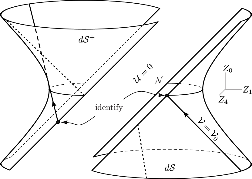
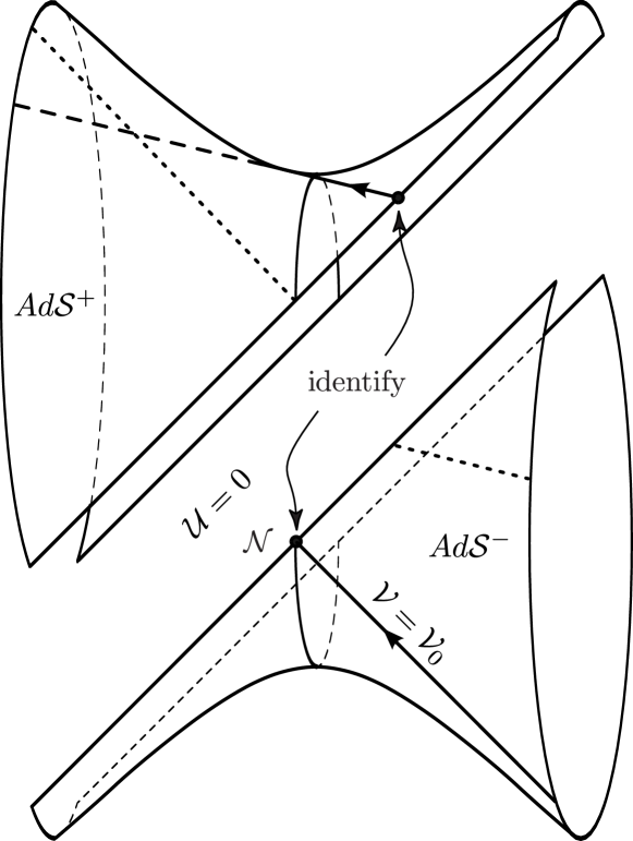
Figure 2: The null geodesic generators of (A)dS and their interaction with the impulisve wave.

The upshot is that these ‘broken geodesic generators’ basically are the coordinate lines of the coordinate system in which the metric becomes continuous, i.e., (2.2). But we do not only have these limiting geodesics at our hand but also the generalized geodesics of Theorem 3.1. This will allow us to geometrically regularize the transformation, which we will explicitly do next.

4.2 The geometrically regularized transformation

Using the ideas laid out above we now give the explicit form of the transformation in nonlinear generalized functions. To begin with, note that we only have carried out the nonlinear distributional analysis of the geodesics in the $5D$-form. Therefore we split up the transformation in the following way: starting from the ‘continuous’ $4D$-coordinates $(u,v,Z)\equiv(u,v,X,Y)$ of (2.2) we first use the transformation (2.9) to go to the $5D$-coordinates $(U,V,Z_{p})$. Then we use the regularised geodesics to transform

$$(U,V,Z_{p})\mapsto T_{\varepsilon}(U,V,Z_{p}):=\gamma^{\varepsilon}_{5D}[V,Z_{p}](U)=:(\bar{U}_{\varepsilon},\bar{V}_{\varepsilon},\bar{Z}_{p\varepsilon})\,,$$ (4.14)

where $[(\gamma^{\varepsilon}_{5D}[V,Z_{p}])_{\varepsilon}]$ are the generalized solutions of the geodesic equations provided by Theorem 3.1 with data constructed from the seed geodesic $\gamma^{g}_{5D}$ of (4.3), i.e., the null generator with data $(V,Z_{p},\dot{V},\dot{Z}_{p})$ as in (4.4), but now derived from $(v,X,Y)$ instead of $({\mathcal{V}}_{0},x_{0},y_{0})$. We will specify this data explicitly below but first we turn to the final final part of the transformation. For this we use the inverse of (2.9), i.e.,

$${\mathcal{U}}=\Omega\bar{U}\,,\qquad{\mathcal{V}}=\Omega\bar{V}\,,\qquad x=\Omega\bar{Z}_{2}\,,\qquad y=\Omega\bar{Z}_{3}\,,\qquad\hbox{with}\qquad\Omega=\frac{2a}{\bar{Z}_{4}+a}\,,$$ (4.15)

componentwise (that is for fixed $\varepsilon$), to go from the $5D$-coordinates $(\bar{U}_{\varepsilon},\bar{V}_{\varepsilon},\bar{Z}_{p\varepsilon})$ to $4D$ coordinates $({\mathcal{U}}_{\varepsilon},{\mathcal{V}}_{\varepsilon},x_{\varepsilon},y_{\varepsilon})$, which provide a regularisation of the $4D$ ‘distributional’ system. That is, overall the transformation we are going to employ takes the form

$$\left(\begin{array}[]{c}u\\ v\\ X\\ Y\end{array}\right)\quad\overset{\eqref{CoordTrans_4D_to_5D}}{\longmapsto}\quad\left(\begin{array}[]{c}U\\ V\\ Z_{p}\end{array}\right)\quad\overset{T_{\varepsilon}}{\longmapsto}\quad\gamma^{\varepsilon}_{5D}[V,Z_{p}](U)\ =\ \left(\begin{array}[]{c}\bar{U}_{\varepsilon}\\ \bar{V}_{\varepsilon}\\ \bar{Z}_{p_{\varepsilon}}\end{array}\right)\quad\overset{\eqref{CoordTrans_5D_to_4D}}{\longmapsto}\quad\left(\begin{array}[]{c}{\mathcal{U}}_{\varepsilon}\\ {\mathcal{V}}_{\varepsilon}\\ x_{\varepsilon}\\ y_{\varepsilon}\end{array}\right)\,.$$ (4.30)

This is the sensible geometric regularisation of the ‘discontinuous transformation’ (4.13), which we have been aiming for.

Since the first and the third map in the overall transformation (4.30) are (classical smooth) diffeomorphisms it is sufficient to restrict our nonlinear distributional analysis of the transformation to $T_{\varepsilon}$. Therefore we do not need to take into account that the data $(V,Z_{p},\dot{V},\dot{Z}_{p})$ of (4.3) is derived from the $4D$-data $(v,X,Y)$ (according to (4.4)). We only have to observe the special form of the null geodesic generators $\gamma^{g}_{5D}$. In fact, we have

$$\gamma^{g}_{5D}(0)=(0,V,Z_{p})\quad\text{and consequently}\quad\dot{\gamma}^{g}_{5D}(0)=\Big{(}1,\,-\beta V,\,-\beta Z_{i},\,-\beta(Z_{4}+a)\Big{)}\,,$$ (4.31)

where $\beta=-(\Lambda/6)\,\Omega V$, and $\Omega=(2a)/(Z_{4}+a)$.

Let us now derive the explicit form of $T_{\varepsilon}$. According to (4.30) we set

$$T_{\varepsilon}(U,V,Z_{p})=\gamma^{\varepsilon}_{5D}[V,Z_{p}](U),$$ (4.32)

where $\gamma^{\varepsilon}_{5D}$ solves ((1)) with data

$$\gamma^{\varepsilon}_{5D}(U=-\varepsilon)=\gamma^{g}_{5D}(-\varepsilon)\quad\text{and}\quad\dot{\gamma}^{\varepsilon}_{5D}(U=-\varepsilon)=\dot{\gamma}^{g}_{5D}(-\varepsilon)\,,$$ (4.33)

i.e., data constructed from the null geodesic generator $\gamma^{g}_{5D}$ with data (4.31) as seed. Since these data essentially reduce to the four parameters $(V,Z_{p})$, we will refer to $\gamma^{\varepsilon}_{5D}[V,Z_{p}]$ as the global geodesics with data $(V,Z_{p})$. Using (4.31) we find

$$\gamma^{\varepsilon}_{5D}(-\varepsilon) =\Big{(}-\varepsilon,\,(1+\beta\varepsilon)V,\,(1+\beta\varepsilon)Z_{i},\,(1+\beta\varepsilon)Z_{4}+\beta\varepsilon a\Big{)},\ \text{and}$$ (4.34)

$$\dot{\gamma}^{\varepsilon}_{5D}(-\varepsilon) =\Big{(}1,\,-\beta V,\,-\beta Z_{i},\,-\beta(Z_{4}+a)\Big{)}\,.$$ (4.35)

Now we may write $\gamma^{\varepsilon}_{5D}[V,Z_{p}](U)=(\bar{U}_{\varepsilon},\bar{V}_{\varepsilon},\bar{Z}_{p_{\varepsilon}})[V,Z_{p}](U)$ by using ((1)) as

$$\gamma^{\varepsilon}_{5D}[V,Z_{p}](U)=\gamma^{\varepsilon}_{5D}[V,Z_{p}](-\varepsilon)+\dot{\gamma}^{\varepsilon}_{5D}[V,Z_{p}](-\varepsilon)\,(U+\varepsilon)+\int\limits_{-\varepsilon}^{U}\int\limits_{-\varepsilon}^{s}\,\ddot{\gamma}^{\varepsilon}_{5D}[V,Z_{p}](r)\,dr\,ds\,.$$ (4.36)

To do so explicitly we use the following abbreviations for the terms appearing on the r.h.s. of ((1))

$$\Delta_{\varepsilon}(r) :=\frac{1}{2}\,{\dot{\bar{U}}_{\varepsilon}^{2}(r)}\,\tilde{G}_{\varepsilon}(r)-\dot{\bar{U}}_{\varepsilon}(r)\,\frac{d}{dr}\,\Big{(}H\big{(}\bar{Z}_{p\varepsilon}(r)\big{)}\,\delta_{\varepsilon}\big{(}\bar{U}_{\varepsilon}(r)\big{)}\,\bar{U}_{\varepsilon}(r)\Big{)}\ \text{with}$$ (4.37)

$$\tilde{G}_{\varepsilon}(r) :=\delta^{pq}\,H_{,p}\big{(}\bar{Z}_{w\varepsilon}(r)\big{)}\,\delta_{\varepsilon}\big{(}\bar{U}_{\varepsilon}(r)\big{)}\,\bar{Z}_{q\varepsilon}(r)+H\big{(}\bar{Z}_{w\varepsilon}(r)\big{)}\,\delta^{\prime}_{\varepsilon}\big{(}\bar{U}_{\varepsilon}(r)\big{)}\,\bar{U}_{\varepsilon}(r)\,,$$ (4.38)

$$N_{\varepsilon}(r) :=\sigma\,a^{2}-\bar{U}_{\varepsilon}^{2}(r)\,H\big{(}\bar{Z}_{p\varepsilon}(r)\big{)}\,\delta_{\varepsilon}(\bar{U}_{\varepsilon}(r))\,.$$ (4.39)

With this we find

$$\bar{U}_{\varepsilon}[V,Z_{p}](U) =U-\int\limits_{-\varepsilon}^{U}\int\limits_{-\varepsilon}^{s}\frac{\Delta_{\varepsilon}(r)}{N_{\varepsilon}(r)}\ \bar{U}_{\varepsilon}(r)\ {\rm{d}}r{\rm{d}}s\,,$$ (4.40)

$$\bar{V}_{\varepsilon}[V,Z_{p}](U) =(1-\beta U)V+\frac{1}{2}\,\int\limits_{-\varepsilon}^{U}\int\limits_{-\varepsilon}^{s}H(\bar{Z}_{p\varepsilon})(r)\,\delta^{\prime}_{\varepsilon}\big{(}\bar{U}_{\varepsilon}(r)\big{)}\,\dot{\bar{U}}_{\varepsilon}^{2}(r)\ {\rm{d}}r{\rm{d}}s$$

$$\qquad+\int\limits_{-\varepsilon}^{U}\int\limits_{-\varepsilon}^{s}\delta^{pq}\,H_{,p}\big{(}\bar{Z}_{w\varepsilon}(r)\big{)}\,\delta_{\varepsilon}\big{(}\bar{U}_{\varepsilon}(r)\big{)}\,\dot{\bar{Z}}_{q\varepsilon}(r)\,\dot{\bar{U}}_{\varepsilon}(r)\ {\rm{d}}r{\rm{d}}s$$ (4.41)

$$\qquad-\int\limits_{-\varepsilon}^{U}\int\limits_{-\varepsilon}^{s}\frac{\Delta_{\varepsilon}(r)}{N_{\varepsilon}(r)}\ \Big{(}\bar{V}_{\varepsilon}(r)+H\big{(}\bar{Z}_{p\varepsilon}(r)\big{)}\,\delta_{\varepsilon}\big{(}\bar{U}_{\varepsilon}(r)\big{)}\,\bar{U}_{\varepsilon}(r)\Big{)}\ {\rm{d}}r{\rm{d}}s\,,$$

$$\bar{Z}_{i\varepsilon}[V,Z_{p}](U) =(1-\beta U)Z_{i}+\frac{1}{2}\ \int\limits_{-\varepsilon}^{U}\int\limits_{-\varepsilon}^{s}H_{,i}\big{(}\bar{Z}_{p\varepsilon}(r)\big{)}\,\delta_{\varepsilon}\big{(}\bar{U}_{\varepsilon}(r)\big{)}\,\dot{\bar{U}}_{\varepsilon}^{2}(r)\ {\rm{d}}r{\rm{d}}s$$

$$\qquad-\int\limits_{-\varepsilon}^{U}\int\limits_{-\varepsilon}^{s}\frac{\Delta_{\varepsilon}(r)}{N_{\varepsilon}(r)}\ \bar{Z}_{i\varepsilon}(r)\ {\rm{d}}r{\rm{d}}s\,,$$ (4.42)

$$\bar{Z}_{4\varepsilon}[V,Z_{p}](U) =(1-\beta U)\ \frac{2a}{\alpha}-a+\frac{\sigma}{2}\ \int\limits_{-\varepsilon}^{U}\int\limits_{-\varepsilon}^{s}H_{,4}\big{(}\bar{Z}_{p\varepsilon}(r)\big{)}\,\delta_{\varepsilon}\big{(}\bar{U}_{\varepsilon}(r)\big{)}\,\dot{\bar{U}}_{\varepsilon}^{2}(r)\ {\rm{d}}r{\rm{d}}s$$

$$\qquad-\int\limits_{-\varepsilon}^{U}\int\limits_{-\varepsilon}^{s}\frac{\Delta_{\varepsilon}(r)}{N_{\varepsilon}(r)}\ \bar{Z}_{4\varepsilon}(r)\ {\rm{d}}r{\rm{d}}s\,.$$ (4.43)

Finally, we observe that the ‘data parts’ of the above equations in fully explicit form read

$$(1-\beta U)V =\Big{(}1+\frac{\Lambda}{3}\ \frac{a}{Z_{4}+a}\ V\,U\Big{)}\ V\,,$$ (4.44)

$$(1-\beta U)Z_{i} =\Big{(}1+\frac{\Lambda}{3}\ \frac{a}{Z_{4}+a}\ V\,U\Big{)}\ Z_{i}\,,$$ (4.45)

$$(1-\beta U)\ \frac{2a}{\alpha}-a =Z_{4}+a\Big{(}1+\frac{\Lambda}{3}\ V\,U\Big{)}-a\,.$$ (4.46)

5 Analysis of the regularised transformation

In this section we finally establish that the geometrically regularized transformation $(T_{\varepsilon})_{\varepsilon}$ is a representative of a generalized diffemorphism $T=[(T_{\varepsilon})_{\varepsilon}]$ in the sense of nonlinear distributional geometry and thus give a precise mathematical meaning to the physical equivalence of the distributional and the continuous form of the metric.

The main issue here is of course the subtle interplay between the image of $T_{\varepsilon}$ and the domain of the inverse. In particular, we have to make sure that the intersection of all images $\cap_{\varepsilon>0}\,\mathrm{im}T_{\varepsilon}$ contains an open set, which can act as the domain of the inverse. More precisely we use the following definition.

Definition 5.1 (Generalized diffeomorphism).

Let $\Omega\subseteq\mathbb{R}^{n}$ be open. We call $T\in{\mathcal{G}}[\Omega,\mathbb{R}^{n}]$ a generalized diffeomorphism if there exists $\eta>0$ such that

1. There exists a representative $(t_{\varepsilon})_{\varepsilon}$ of $T$ such that $t_{\varepsilon}\colon\Omega\rightarrow t_{\varepsilon}(\Omega)=:\tilde{\Omega}_{\varepsilon}$ is a diffeomorphism for all $\varepsilon\leq\eta$ and there exists $\tilde{\Omega}\subseteq\mathbb{R}^{n}$ open with $\tilde{\Omega}\subseteq\bigcap_{\varepsilon\leq\eta}\tilde{\Omega}_{\varepsilon}$.

2. The inverses $(t_{\varepsilon}^{-1})_{\varepsilon}$ are moderate and c-bounded, i.e., $(t_{\varepsilon}^{-1})_{\varepsilon}\in{\mathcal{G}}[\tilde{\Omega},\mathbb{R}^{n}]$ and there exists $\Omega_{1}\subseteq\mathbb{R}^{n}$ open, $\Omega_{1}\subseteq\bigcap_{\varepsilon\leq\eta}t_{\varepsilon}^{-1}(\tilde{\Omega})$.

3. Setting $T^{-1}:=[(t_{\varepsilon}^{-1}|_{\tilde{\Omega}})_{\varepsilon}]$, the compositions $T\circ T^{-1}$ and $T^{-1}\circ T|_{\Omega_{1}}$ are elements of ${\mathcal{G}}(\tilde{\Omega},\mathbb{R}^{n})$ respectively ${\mathcal{G}}(\Omega_{1},\mathbb{R}^{n})$. (It is then clear that $T\circ T^{-1}=id_{\tilde{\Omega}}$ and $T^{-1}\circ T|_{\Omega_{1}}=id_{\Omega_{1}})$.

This definition, of course, extends the smooth theory, cf. [1, Supplement 2.5A] for a version ‘quantifying’ the neighbourhoods in the classical inverse function theorem.

We will show that $T$ is a generalized diffeomorphism and we will split up this task in two subsections.

5.1 $T$ as a generalized function

To begin with, we have to establish that the regularised transformation $T_{\varepsilon}$ gives rise to a c-bounded generalized function on $\mathbb{R}^{5}$, more precisely that $[(T_{\varepsilon})_{\varepsilon}]\in{\mathcal{G}}[\mathbb{R}^{5},\mathbb{R}^{5}]$. Recall that by (4.32) we have $T_{\varepsilon}(U,V,Z_{p})=\gamma^{\varepsilon}_{5D}[V,Z_{p}](U)$ and that so far we have only considered $\gamma^{\varepsilon}_{5D}$ as a function of $U$. Indeed, Theorem 3.1 guarantees that $[(\gamma^{\varepsilon}_{5D})_{\varepsilon}]\in{\mathcal{G}}[\mathbb{R},\mathbb{R}^{5}]$, but now we have to additionally deal with the dependence of $\gamma^{\varepsilon}_{5D}[V,Z_{p}](U)$ on $V$ and $Z_{p}$.

We first establish an appropriate ‘uniformity of domains’ of $\gamma^{\varepsilon}_{5D}$ in $(V,Z_{p})$. To this end we have to delve into the fixed point argument of [43, Sec. III A] that leads to the construction of a local solution candidate for the geodesic equation. Recall from there, or observe from (3.2) that the $V$-equation decouples from the system and can simply be integrated after the rest of the system has been solved. So we only have to consider the existence statement [43, Prop. 3.2] which guarantees a local solution for small $\varepsilon$ of a model system which neglects the $V$-equation. There the existence of unique solutions is established on the interval $[\alpha_{\varepsilon},\alpha_{\varepsilon}+\eta]$ when $\varepsilon\leq\varepsilon_{0}$, where $\varepsilon_{0}$ and $\eta$ have to satisfy the explicit bounds given in equations [43, (29), (30)] and the unnumbered equation on top of p. 9, respectively. These are explicit bounds in terms of the coefficient functions of the system (local $L^{\infty}$-norms of $H$ and $DH$, as well as the $L^{1}$-norm of $\rho$ and $\rho^{\prime}$) and the seed data. The latter in our case simplifies to the $Z_{p}$-components of

$$\gamma^{g}_{5D}(0)=(0,V,Z_{p}),\quad\dot{\gamma}^{g}_{5D}(0)=\Big{(}1,\,-\beta V,\,-\beta Z_{i},\,-\beta(Z_{4}+a)\Big{)}\,,$$ (5.1)

cf. (4.31). By inspection it becomes obvious that these estimates can be maintained if the seed data (there $x^{0}$ and $\dot{x}^{0}$) vary in a neighborhood (here of $Z_{p}$) and that hence $\eta$ and $\varepsilon_{0}$ can be chosen uniformly on compact neighbourhoods of $Z_{p}$. Observing that for $\alpha_{\varepsilon}+\eta\geq\beta_{\varepsilon}$ the solution again reduces to a background geodesic and using a simple exhaustion argument as in [10, Prop. 4.3] we obtain the following result.

Lemma 5.2 (Uniform domains).

Given any compact set $K$ in $\mathbb{R}^{4}$ there is $\varepsilon_{0}(K)$ such that $\gamma^{\varepsilon}_{5D}[V,Z_{p}]$ is the unique globally defined geodesic of (4.32) for all data $(V,Z_{p})\in K$ and for all $\varepsilon\leq\varepsilon_{0}(K)$.

Next we deal with the c-boundedness of $\gamma^{\varepsilon}_{5D}[V,Z_{p}]$. Observe that c-boundedness as a function of $U$ is already provided by Theorem 3.1, essentially proved in [45, Prop. 4.1 and Appendix A]. We now have to see that $\gamma^{\varepsilon}_{5D}$ is also uniformly bounded if we vary $V$ and $Z_{p}$ in a compact set. This, however, can also be accomplished by an inspection. For the $Z_{p}$-components we have to again look into the fixed point argument, more precisely to [45, Appendix A]. The constant $C_{2}$ of [45, (A.6)] that bounds the solutions again depends on the coefficient functions of the system and the seed data. It clearly can be chosen uniform on compact neighbourhoods of the data, that is of $Z_{p}$ as the $U$-speed (there $\dot{u}^{0}$) in our case is anyways fixed to $1$. So we obtain uniform boundedness of $\bar{U}_{\varepsilon}$, and $\bar{Z}_{p\varepsilon}$ on compact subsets, as well as of the derivatives $\dot{\bar{U}}_{\varepsilon}=\partial_{U}\bar{U}_{\varepsilon}$, and $\dot{\bar{Z}}_{p\varepsilon}=\partial_{U}\bar{Z}_{p\varepsilon}$. Finally, for the $V$-component we have to inspect the boundedness result in [45, Prop. 4.1(iii)]. Again it is easily seen that the constants in [45, (4.1)] vary uniformly if $(V,Z_{p})$ vary in a compact set. In total we have established the following ‘uniformity of bounds’ result.

Lemma 5.3 (Uniform bounds).

The global geodesics $\gamma^{\varepsilon}_{5D}[V,Z_{p}]$ of (4.32) are uniformly bounded on compact subsets of $\mathbb{R}^{5}$ for $\varepsilon$ small enough. In addition such bounds also apply to $\partial_{U}\bar{U}_{\varepsilon}$, and $\partial_{U}\bar{Z}_{p\varepsilon}$.

The final task in this subsection is to establish moderateness. We first derive a number of asymptotic estimates which we will also need later on.

Lemma 5.4.

Denoting by $\nabla$ any of the derivatives $\partial_{V}$ and $\partial_{Z_{p}}$ we have in the regularisation strip $-\varepsilon\leq r\leq\beta_{\varepsilon}$ and $(V,Z_{p})$ varying in a compact set

$$N_{\varepsilon}(r) =O(1),\quad\tilde{G}_{\varepsilon}(r)=O(\frac{1}{\varepsilon}),\quad\Delta_{\varepsilon}(r)=O(\frac{1}{\varepsilon})\,,$$ (5.2)

$$\nabla N_{\varepsilon} =O(1)\nabla\bar{U}_{\varepsilon}+O(\varepsilon)\nabla\bar{Z}_{p\varepsilon}\,,$$ (5.3)

$$\nabla G_{\varepsilon}(r) =O(\frac{1}{\varepsilon^{2}})\nabla\bar{U}_{\varepsilon}+O(\frac{1}{\varepsilon})\nabla\bar{Z}_{p\varepsilon}\,,$$ (5.4)

$$\nabla\Delta_{\varepsilon} =O(\frac{1}{\varepsilon^{2}})\nabla\bar{U}_{\varepsilon}+O(\frac{1}{\varepsilon})(\nabla\bar{Z}_{p\varepsilon}+\nabla\dot{\bar{U}}_{\varepsilon})+O(1)\nabla\dot{\bar{Z}}_{p\varepsilon}\,.$$ (5.5)

Proof.

The estimates (5.2) follow direct from the definitions (4.37)–(4.39) observing the boundedness results of Lemma 5.3. Similarly we obtain

$$\nabla N_{\varepsilon}(r)=-2\bar{U}_{\varepsilon}\nabla\bar{U}_{\varepsilon}H\delta_{\varepsilon}-\bar{U}_{\varepsilon}^{2}DH\nabla Z_{p\varepsilon}\delta_{\varepsilon}-\bar{U}_{\varepsilon}^{2}H\delta^{\prime}_{\varepsilon}\nabla\bar{U}_{\varepsilon}\\ =O(1)\nabla\bar{U}_{\varepsilon}+O(\varepsilon)\nabla\bar{Z}_{p\varepsilon}\,,$$ (5.6)

where we have omitted to write out the arguments of $H$, $\delta_{\varepsilon}$ and the components of $\gamma^{\varepsilon}_{5D}[V,Z_{p}]$ explicitly. The result on $\nabla\tilde{G}_{\varepsilon}$ simply follows in a similar vein. Finally to derive the estimate on $\Delta_{\varepsilon}$ first observe that

$$\frac{d}{dr}(H\delta_{\varepsilon}\bar{U}_{\varepsilon}) =O(\frac{1}{\varepsilon})\,,$$ (5.7)

$$\nabla\frac{d}{dr}(H\delta_{\varepsilon}\bar{U}_{\varepsilon}) =O(\frac{1}{\varepsilon^{2}})\nabla\bar{U}_{\varepsilon}+O(\frac{1}{\varepsilon})(\nabla\bar{Z}_{p\varepsilon}+\nabla\dot{\bar{U}}_{\varepsilon})+O(1)\nabla\dot{\bar{Z}}_{p\varepsilon}\,.$$ (5.8)

Now the result again follows along the same lines. ∎

The next step is to apply Lemma 5.4 to obtain estimates on the first order derivatives of $\bar{U}_{\varepsilon}$, $\dot{\bar{U}}_{\varepsilon}$, $\bar{Z}_{p\varepsilon}$, and $\dot{\bar{Z}}_{p\varepsilon}$. More precisely we have.

Lemma 5.5 (Asymptotic estimates on the first order derivatives).

We have in the regularisation strip $-\varepsilon\leq r\leq\beta_{\varepsilon}$ and $(V,Z_{p})$ varying in a compact set

$$\partial_{V}\bar{U}_{\varepsilon}=O(\varepsilon^{2})\,,\quad \partial_{V}(\dot{\bar{U}}_{\varepsilon},\bar{Z}_{p\varepsilon})=O(\varepsilon)\,,\quad \partial_{V}\dot{\bar{Z}}_{p\varepsilon}=O(1)\,,$$ (5.9)

$$\partial_{Z_{q}}\bar{U}_{\varepsilon}=O(\varepsilon)\,,\quad \partial_{Z_{q}}(\dot{\bar{U}}_{\varepsilon},\bar{Z}_{p\varepsilon})=O(1)\,,\ \partial_{Z_{q}}\dot{\bar{Z}}_{p\varepsilon}=O(1/\varepsilon)\,,$$ (5.10)

as well as

$$\partial_{V}N_{\varepsilon}=O(\varepsilon^{2})\,,\quad\partial_{Z_{p}}N_{\varepsilon}=O(\varepsilon)\,,\quad\partial_{V}\Delta_{\varepsilon}=O(1)\,,\quad\partial_{Z_{p}}\Delta_{\varepsilon}=O(1/\varepsilon)\,.$$ (5.11)

Proof.

Since here the $\partial_{V}$- and $\partial_{Z_{p}}$-derivatives will part ways we introduce the following notation: First we do not distinguish between the individual $\partial_{Z_{p}}$’s ($p=1,2,3$) and simply write $\partial_{Z}$. Moreover, we will write $\nabla=(\nabla_{1},\nabla_{2})=(\partial_{V},\partial_{Z})$ and also use the notation $\nabla_{A}$ ($A=1,2$).

We aim for a Gronwall estimate using the integral representation of the respective components of the geodesics (4.40), (4.42), and (4.43). However, we will do so in a nested way starting with $\nabla\bar{U}_{\varepsilon}$, $\nabla\dot{\bar{U}}_{\varepsilon}$, and $\nabla\bar{Z}_{p\varepsilon}$, while leaving $\nabla\dot{\bar{Z}}_{p\varepsilon}$ for later treatment. Setting

$$\Psi_{A}:=\max\Big{(}|\nabla_{A}\bar{U}_{\varepsilon}|,|\nabla_{A}\dot{\bar{U}}_{\varepsilon}|,|\nabla_{A}\bar{Z}_{p\varepsilon}|\Big{)}\,,$$ (5.12)

we obtain from (4.40) and from (5.3), (5.5)

$$|\nabla_{A}\bar{U}_{\varepsilon}|\, =\,\int\limits_{-\varepsilon}^{\beta_{\varepsilon}}\int\limits_{-\varepsilon}^{\beta_{\varepsilon}}\Big{(}O\big{(}\frac{1}{\varepsilon}\big{)}\,\Psi_{A}+O(\varepsilon)|\nabla_{A}\dot{\bar{Z}}_{p\varepsilon}|\Big{)}\,,$$ (5.13)

$$|\nabla_{A}\dot{\bar{U}}_{\varepsilon}|\, =\,\int\limits_{-\varepsilon}^{\beta_{\varepsilon}}\Big{(}O\big{(}\frac{1}{\varepsilon}\big{)}\,\Psi_{A}+O(\varepsilon)|\nabla_{A}\dot{\bar{Z}}_{p\varepsilon}|\Big{)}\,.$$ (5.14)

Similarly, using (4.42), (4.43) we obtain by a lengthy calculation

$$|\partial_{V}\bar{Z}_{p\varepsilon}|\, =\,O(\varepsilon)+\int\limits_{-\varepsilon}^{\beta_{\varepsilon}}\int\limits_{-\varepsilon}^{\beta_{\varepsilon}}\Big{(}O\big{(}\frac{1}{\varepsilon}\big{)}\,\Psi_{1}+O(\varepsilon)|\partial_{V}\dot{\bar{Z}}_{p\varepsilon}|\Big{)}\,,$$ (5.15)

$$|\partial_{Z}\bar{Z}_{p\varepsilon}|\, =\,O(1)+\int\limits_{-\varepsilon}^{\beta_{\varepsilon}}\int\limits_{-\varepsilon}^{\beta_{\varepsilon}}\Big{(}O\big{(}\frac{1}{\varepsilon}\big{)}\,\Psi_{2}+O(\varepsilon)|\partial_{Z}\dot{\bar{Z}}_{p\varepsilon}|\Big{)}\,.$$ (5.16)

Summing up we therefore have

$$\Psi_{1}\, =\,O(\varepsilon)+\int\limits_{-\varepsilon}^{\beta_{\varepsilon}}\Big{(}O\big{(}\frac{1}{\varepsilon}\big{)}\Psi_{1}+O(\varepsilon)|\partial_{V}\dot{\bar{Z}}_{p\varepsilon}|\Big{)}\,,$$ (5.17)

$$\Psi_{2}\, =\,O(1)+\int\limits_{-\varepsilon}^{\beta_{\varepsilon}}\Big{(}O\big{(}\frac{1}{\varepsilon}\big{)}\Psi_{2}+O(\varepsilon)|\partial_{Z}\dot{\bar{Z}}_{p\varepsilon}|\Big{)}\,,$$ (5.18)

and a first appeal to the Gronwall inequality gives

$$\Psi_{1}\,=\,O(\varepsilon)\,\Big{(}1+\int\limits_{-\varepsilon}^{\beta_{\varepsilon}}|\partial_{V}\dot{\bar{Z}}_{p\varepsilon}|\Big{)}\,,\quad\mbox{and}\quad\Psi_{2}\,=\,O(1)+O(\varepsilon)\int\limits_{-\varepsilon}^{\beta_{\varepsilon}}|\partial_{Z}\dot{\bar{Z}}_{p\varepsilon}|\,.$$ (5.19)

Next we turn to $\nabla\dot{\bar{Z}}_{p\varepsilon}$ for which we find, again from (4.42), (4.43), and (5.3), (5.5)

$$|\partial_{V}\dot{\bar{Z}}_{p\varepsilon}|\, =\,\int\limits_{-\varepsilon}^{\beta_{\varepsilon}}O\big{(}\frac{1}{\varepsilon^{2}}\big{)}\Psi_{1}+\int\limits_{-\varepsilon}^{\beta_{\varepsilon}}O(1)|\partial_{V}\dot{\bar{Z}}_{p\varepsilon}|\,=\,O(1)+\int\limits_{-\varepsilon}^{\beta_{\varepsilon}}O(1)|\partial_{V}\dot{\bar{Z}}_{p\varepsilon}|\,,$$ (5.20)

$$|\partial_{Z}\dot{\bar{Z}}_{p\varepsilon}|\, =\,O(1)+\int\limits_{-\varepsilon}^{\beta_{\varepsilon}}O\big{(}\frac{1}{\varepsilon^{2}}\big{)}\Psi_{2}+\int\limits_{-\varepsilon}^{\beta_{\varepsilon}}O(1)|\partial_{Z}\dot{\bar{Z}}_{p\varepsilon}|\,=\,O\big{(}\frac{1}{\varepsilon}\big{)}+\int\limits_{-\varepsilon}^{\beta_{\varepsilon}}O(1)|\partial_{Z}\dot{\bar{Z}}_{p\varepsilon}|\,,$$ (5.21)

where in both lines the second equality follows from (5.19). Now a second appeal to the Gronwall inequality hence leaves us with

$$|\partial_{V}\dot{\bar{Z}}_{p\varepsilon}|=O(1)\,,\quad\text{and}\quad|\partial_{Z}\dot{\bar{Z}}_{p\varepsilon}|=O\big{(}\frac{1}{\varepsilon}\big{)}\,,$$ (5.22)

which already gives the claim on $\nabla\dot{\bar{Z}}_{p\varepsilon}$. Also, it allows us to improve the estimates (5.19) on $\Psi_{A}$ to

$$\Psi_{1}=O(\varepsilon)\,,\quad\mbox{and}\quad\Psi_{2}=O(1)\,,$$ (5.23)

which upon inserting into (5.13)–(5.16) gives the claims on $\partial\bar{U}_{\varepsilon}$, $\partial\dot{\bar{U}}_{\varepsilon}$, and $\partial\bar{Z}_{\varepsilon}$. Finally, we insert these estimates into (5.3) and (5.5) to obtain (5.11). ∎

Lemma 5.6 (Asymptotic estimates on the higher order derivatives).

Denoting by $\nabla$ any of the derivatives $\partial_{V}$ and $\partial_{Z_{p}}$ we have in the regularisation strip $-\varepsilon\leq r\leq\beta_{\varepsilon}$ and $(V,Z_{p})$ varying in a compact set that for any $n$ there is $N$ such that

$$\nabla^{n}(\bar{U}_{\varepsilon},\dot{\bar{U}}_{\varepsilon},\bar{Z}_{p\varepsilon},\dot{\bar{Z}}_{p\varepsilon})\,=\,O(\varepsilon^{-N})\,.$$ (5.24)

Proof.

We proceed by induction. Clearly Lemma 5.5 provides the basis of induction. So assume that we have $\nabla^{n}(\bar{U}_{\varepsilon},\dot{\bar{U}}_{\varepsilon},\bar{Z}_{p\varepsilon},\dot{\bar{Z}}_{p\varepsilon})=O(\varepsilon^{-M})$ for some $M$. We aim for again a nested Gronwall argument for the highest order derivatives. Staring with $\bar{U}_{\varepsilon}$, and $\dot{\bar{U}}_{\varepsilon}$, we find using the integral representation (4.40)

$$\nabla^{n+1}\bar{U}_{\varepsilon}\, =\,\int\limits_{-\varepsilon}^{\beta_{\varepsilon}}O(\varepsilon^{2})\nabla^{n+1}\Big{(}\frac{\Delta_{\varepsilon}}{N_{\varepsilon}}\Big{)}+\int\limits_{-\varepsilon}^{\beta_{\varepsilon}}O(1)\nabla^{n+1}\bar{U}_{\varepsilon}+O(\varepsilon^{-N})\,,$$ (5.25)

$$\nabla^{n+1}\dot{\bar{U}}_{\varepsilon}\, =\,\int\limits_{-\varepsilon}^{\beta_{\varepsilon}}O(\varepsilon)\nabla^{n+1}\Big{(}\frac{\Delta_{\varepsilon}}{N_{\varepsilon}}\Big{)}+\int\limits_{-\varepsilon}^{\beta_{\varepsilon}}O\big{(}\frac{1}{\varepsilon}\big{)}\nabla^{n+1}\bar{U}_{\varepsilon}+O(\varepsilon^{-N})\,,$$ (5.26)

where we have only retained the highest order terms explicitly and estimated all lower order terms by some large inverse power of $\varepsilon$. Next we deal with the term $\nabla^{n+1}\bar{Z}_{p\varepsilon}$ for which we find from (4.42), and (4.43)

$$\nabla^{n+1}\bar{Z}_{p\varepsilon}\,=\,\int\limits_{-\varepsilon}^{\beta_{\varepsilon}}\left(O\big{(}\frac{1}{\varepsilon}\big{)}\,\Big{(}\nabla^{n+1}\bar{U}_{\varepsilon}+\nabla^{n+1}\dot{\bar{U}}_{\varepsilon}+\nabla^{n+1}\bar{Z}_{p\varepsilon}\Big{)}+O(\varepsilon)\nabla^{n+1}\Big{(}\frac{\Delta_{\varepsilon}}{N_{\varepsilon}}\Big{)}\right)+O(\varepsilon^{-N})\,,$$ (5.27)

simply collecting all lower order terms in the final $O(\varepsilon^{-N})$-estimate. Observe, that the (critical) term involving $\delta_{\varepsilon}(\bar{U}_{\varepsilon})$ does not produce any (high) inverse powers of $\varepsilon$ in the highest order terms $\nabla^{n+1}(\bar{U}_{\varepsilon},\dot{\bar{U}}_{\varepsilon},\bar{Z}_{p\varepsilon})$.

Now we set $\Psi=\max(|\nabla^{n+1}\bar{U}_{\varepsilon}|,|\nabla^{n+1}\dot{\bar{U}}_{\varepsilon}|,|\nabla^{n+1}\bar{Z}_{p\varepsilon}|)$ and obtain by collecting the above estimates

$$\Psi\,=\,\int\limits_{-\varepsilon}^{\beta_{\varepsilon}}\left(O(\varepsilon)\nabla^{n+1}\Big{(}\frac{\Delta_{\varepsilon}}{N_{\varepsilon}}\Big{)}+O\big{(}\frac{1}{\varepsilon}\big{)}\Psi\right)+O(\varepsilon^{-N})\,,$$ (5.28)

and so by a first application of Gronwall’s inequality

$$\Psi\,=\,O(\varepsilon^{2})\nabla^{n+1}\Big{(}\frac{\Delta_{\varepsilon}}{N_{\varepsilon}}\Big{)}+O(\varepsilon^{-N})\,.$$ (5.29)

Next we use the integral representations to obtain the following estimate on the $(n+1)$-st derivative of the fraction $\Delta_{\varepsilon}/N_{\varepsilon}$

$$\nabla^{n+1}\Big{(}\frac{\Delta_{\varepsilon}}{N_{\varepsilon}}\Big{)}\, =\,O\big{(}\frac{1}{\varepsilon^{2}}\big{)}\nabla^{n+1}\bar{U}_{\varepsilon}+O\big{(}\frac{1}{\varepsilon}\big{)}\Big{(}\nabla^{n+1}\dot{\bar{U}}_{\varepsilon}+\nabla^{n+1}\bar{Z}_{p\varepsilon}\Big{)}+O(1)\nabla^{n+1}\dot{\bar{Z}}_{p\varepsilon}+O(\varepsilon^{-N})$$

$$=\,\int\limits_{-\varepsilon}^{\beta_{\varepsilon}}O\big{(}\frac{1}{\varepsilon}\big{)}\nabla^{n+1}\Big{(}\frac{\Delta_{\varepsilon}}{N_{\varepsilon}}\Big{)}\ +O(1)\nabla^{n+1}\dot{\bar{Z}}_{p\varepsilon}+O(\varepsilon^{-N})\,,$$ (5.30)

where we have used the estimates (5.28), (5.29). So another appeal to Gronwall’s inequality yields

$$\nabla^{n+1}\Big{(}\frac{\Delta_{\varepsilon}}{N_{\varepsilon}}\Big{)}\,=\,O(1)\nabla^{n+1}\dot{\bar{Z}}_{p\varepsilon}+O(\varepsilon^{-N})\,.$$ (5.31)

Inserting this back into the $\Psi$-estimate (5.29) we find

$$\Psi\,=\,O(\varepsilon^{2})\nabla^{n+1}\dot{\bar{Z}}_{p\varepsilon}+O(\varepsilon^{-N})\,.$$ (5.32)

Finally, we turn to the term $\nabla^{n+1}\dot{\bar{Z}}_{p\varepsilon}$, for which we find again from the integral representation (4.42), and (4.43) (cf. (5.27))

$$\nabla^{n+1}\dot{\bar{Z}}_{p\varepsilon}\, =\,\int\limits_{-\varepsilon}^{\beta_{\varepsilon}}\left(O\big{(}\frac{1}{\varepsilon^{2}}\big{)}\Big{(}\nabla^{n+1}\bar{U}_{\varepsilon}+\nabla^{n+1}\dot{\bar{U}}_{\varepsilon}+\nabla^{n+1}\bar{Z}_{p\varepsilon}\Big{)}+O(1)\nabla^{n+1}\Big{(}\frac{\Delta_{\varepsilon}}{N_{\varepsilon}}\Big{)}\right)+O(\varepsilon^{-N})$$

$$=\int\limits_{-\varepsilon}^{\beta_{\varepsilon}}O(1)\nabla^{n+1}\dot{\bar{Z}}_{p\varepsilon}+O(\varepsilon^{-N})\,,$$ (5.33)

where we have used (5.32) as well as (5.31). So a final appeal to Gronwall’s estimate gives $\nabla^{n+1}\dot{\bar{Z}}_{p\varepsilon}=O(\varepsilon^{-N})$, and, upon inserting into (5.32), $\Psi=O(\varepsilon^{-N})$, which is the claim. ∎

Now we finally obtain moderateness of the transformation. Indeed, we have the following more specific result.

Proposition 5.7 (Moderateness of the transformation).

The transformation $[(T_{\varepsilon})_{\varepsilon}]$ is moderate and hence an element of ${\mathcal{G}}[\mathbb{R}^{5},\mathbb{R}^{5}]$.

Proof.

Recall that we only have to argue inside the regularised wave zone $-\varepsilon\leq\bar{U}_{\varepsilon}\leq\beta_{\varepsilon}$ since outside of it $\gamma^{\varepsilon}_{5D}$ coincides with classical smooth solutions (depending smoothly on $\varepsilon$). The c-boundedness (in this strip) was established in Lemma 5.3 and the moderateness estimates for $\partial_{U}\gamma^{\varepsilon}_{5D}[V,Z_{p}](.)$ are due to Theorem 3.1. The moderateness estimates for the $V$- and $Z_{q}$-derivatives of $\bar{U}_{\varepsilon}$, and $\bar{Z}_{p\varepsilon}$, as well as their mixed $V$-$Z_{q}$-derivatives have been established in Lemma 5.6. The mixed $U$-$V$-$Z_{q}$-derivatives follow suit by iteratively using the differential equation.

Finally, since the $V$-equation is decoupled from the system and $\bar{V}[V,Z_{p}](.)$ is obtained simply by integration of the other components its moderateness is a consequence of moderateness of $(\bar{U},\bar{Z}_{p})$ (and the well-definedness of the respective operations in ${\mathcal{G}}[\mathbb{R}^{n},\mathbb{R}^{m}]$). ∎

5.2 $T$ as generalized diffeomorphism

We will now set out to show that the transformation (4.32), i.e.,

$$(U,V,Z_{p})\mapsto[T_{\varepsilon}](U,V,Z_{p})=[\gamma^{\varepsilon}_{5D}][V,Z_{p}](U)\,\in{\mathcal{G}}[R^{5},\mathbb{R}^{5}]\,,$$ (5.34)

with its components given explicitly by (4.40) - (4.43) gives rise to a locally invertible generalized function $T=[(T_{\varepsilon})_{\varepsilon}]$ on some open set containing the impulsive surface. Hence we will call it a generalised diffeomorphism or generalised coordinate transformation. To do so we will extend the results of the $\Lambda=0$-case of [20] and, in particular, its more mathematically structured presentation in [10]. In fact, inspired by [10] we will decompose the transformation in a convenient way by splitting $T_{\varepsilon}$ into a ‘singular’ and a ‘convergent’ part.

To begin with, fix an open, relatively compact set $W\subseteq\mathbb{R}^{5}$, which will be specified further later, and observe that by Proposition 5.7 $(T_{\varepsilon})$ is moderate and c-bounded and therefore indeed $T:=[(T_{\varepsilon})_{\varepsilon}]\in{\mathcal{G}}[W,\mathbb{R}^{n}]$. We decompose the $\bar{V}_{\varepsilon}$-component into the initial data term $\tilde{V}_{\varepsilon}$ and the integral term, which we label as $h_{\varepsilon}$, so that we may write

$$\bar{V}_{\varepsilon}=\tilde{V}_{\varepsilon}+h_{\varepsilon}\,.$$ (5.35)

To be precise, we have

$$\tilde{V}_{\varepsilon} =(1-\beta U)V\,,$$

$$h_{\varepsilon} =\frac{1}{2}\,\int\limits_{-\varepsilon}^{U}\int\limits_{-\varepsilon}^{s}H(\bar{Z}_{p\varepsilon})(r)\,\delta^{\prime}_{\varepsilon}\big{(}\bar{U}_{\varepsilon}(r)\big{)}\,\dot{\bar{U}}_{\varepsilon}^{2}(r)\ {\rm{d}}r{\rm{d}}s$$

$$\qquad+\int\limits_{-\varepsilon}^{U}\int\limits_{-\varepsilon}^{s}\delta^{pq}\,H_{,p}\big{(}\bar{Z}_{w\varepsilon}(r)\big{)}\,\delta_{\varepsilon}\big{(}\bar{U}_{\varepsilon}(r)\big{)}\,\dot{\bar{Z}}_{q\varepsilon}(r)\,\dot{\bar{U}}_{\varepsilon}(r)\ {\rm{d}}r{\rm{d}}s$$

$$\qquad-\int\limits_{-\varepsilon}^{U}\int\limits_{-\varepsilon}^{s}\frac{\Delta_{\varepsilon}(r)}{N_{\varepsilon}(r)}\ \Big{(}\bar{V}_{\varepsilon}(r)+H\big{(}\bar{Z}_{p\varepsilon}(r)\big{)}\,\delta_{\varepsilon}\big{(}\bar{U}_{\varepsilon}(r)\big{)}\,\bar{U}_{\varepsilon}(r)\Big{)}\ {\rm{d}}r{\rm{d}}s\,.$$

Note that while $h_{\varepsilon}$ does not converge, we have that $h_{\varepsilon}=O(1)$, cf. the proof of Proposition 4.1 in [45] and in particular equations (4.3) and (4.4). At this point we define the converging sequence $s_{\varepsilon}(U,V,Z):=(\bar{U}_{\varepsilon},\tilde{V}_{\varepsilon},\bar{Z}_{i\varepsilon},\bar{Z}_{4\varepsilon})$.

We will use [9, Prop. 3.16 and Thm. 3.59] in order to establish injectivity of $T_{\varepsilon}$, and therefore we need to find the asymptotic behaviour of $DT_{\varepsilon}$ and $Ds_{\varepsilon}$. More specifically, we need to estimate the behaviour of their determinant and all principal minors. The Jacobian of $s_{\varepsilon}$ is

$$Ds_{\varepsilon}=\left(\begin{array}[]{ccccc}1&0&0&0\\ \frac{\Lambda}{3}\frac{a}{Z_{4}+a}V^{2}&1+\frac{2\Lambda}{3}\frac{a}{Z_{4}+a}UV&0&-\frac{\Lambda}{3}\frac{a}{(Z_{4}+a)^{2}}UV^{2}\\ \frac{\Lambda}{3}\frac{a}{Z_{4}+a}VZ_{i}&\frac{\Lambda}{3}\frac{a}{Z_{4}+a}UZ_{i}&1+\frac{\Lambda}{3}\frac{a}{Z_{4}+a}UV&-\frac{\Lambda}{3}\frac{a}{(Z_{4}+a)^{2}}UVZ_{i}\\ \frac{\Lambda}{3}aV&\frac{\Lambda}{3}aU&0&1\\ \end{array}\right)+B\,,$$ (5.36)

where $B$ is a matrix with all entries $O(\varepsilon)$, as we will see in Lemma 5.9 below. For the following we denote

$$\Omega:=\{(U,V,Z)\in\mathbb{R}^{5}:\,\left|\frac{\Lambda}{3}\frac{a}{a+Z_{4}}VU\right|\leq\frac{1}{8}\}\,.$$ (5.37)

Lemma 5.8.

There is $\varepsilon_{0}>0$ such that on any closed rectangular subset of $\Omega$ and for all $\varepsilon<\varepsilon_{0}$, $s_{\varepsilon}$ is injective.

Proof.

For $\varepsilon$ small enough we only have to consider the matrix $Ds_{\varepsilon}-B$. Condition (5.36) guarantees that all principal minors are bounded below by a fixed positive constant on all of $\Omega$. Thus [11, Thm. 4] gives the claimed injectivity. ∎

Outside the regularization strip $\{\alpha_{\varepsilon}\leq U\leq\beta_{\varepsilon}\}$ the transformation defaults to a smooth coordinate transform independent of $\varepsilon$ and hence possesses all the properties needed in the following arguments. Thus we may restrict ourselves to the regularization zone and there $\bar{U}_{\varepsilon}=O(\varepsilon)$ holds. As for $T_{\varepsilon}$, being able to decompose its $V$ component into $\tilde{V}_{\varepsilon}+h_{\varepsilon}$ lets us more easily compute its Jacobian. First, we focus on the regularization strip $\{\alpha_{\varepsilon}\leq U\leq\beta_{\varepsilon}\}$:

Lemma 5.9 (Asymptotics estimates for $\bar{V}_{\varepsilon}$).

We have in the regularisation strip $-\varepsilon\leq r\leq\beta_{\varepsilon}$ and $(V,Z_{p})$ varying in a compact set

$$\bar{V}_{\varepsilon}=O(1),\ \partial_{V}\bar{V}_{\varepsilon}=O(1),\ \partial_{V}h_{\varepsilon}=O(\varepsilon),\ \partial_{Z_{p}}h_{\varepsilon}=O(1)\,.$$ (5.38)

Proof.

The asymptotics of $\bar{V}_{\varepsilon}$ have already been noted in Proposition 5.7. We estimate the $V$-component: As $h_{\varepsilon}$ consists of three integrals, we split up the calculation, writing $h_{\varepsilon}=\frac{1}{2}I_{1}+I_{2}-I_{3}$. Then using the above we obtain that

$$\partial_{V}I_{1}= \int_{-\varepsilon}^{U}\int_{-\varepsilon}^{s}DH(\bar{Z}_{p\varepsilon})\partial_{V}\bar{Z}_{p\varepsilon}\delta^{\prime}(\bar{U}_{\varepsilon})\dot{\bar{U}}_{\varepsilon}^{2}+H(\bar{Z}_{p\varepsilon})\delta^{\prime\prime}(\bar{U}_{\varepsilon})\partial_{V}\bar{U}_{\varepsilon}\dot{\bar{U}}_{\varepsilon}^{2}+H(\bar{Z}_{p\varepsilon})\delta^{\prime}(\bar{U}_{\varepsilon})2\dot{\bar{U}}_{\varepsilon}\partial_{V}\dot{\bar{U}}_{\varepsilon}$$

$$= \int_{-\varepsilon}^{U}\int_{-\varepsilon}^{s}O(1)O(\varepsilon)O(\frac{1}{\varepsilon^{2}})O(1)+O(1)O(\frac{1}{\varepsilon^{3}})O(\varepsilon^{2})O(1)+O(1)O(\frac{1}{\varepsilon^{2}})O(1)O(\varepsilon)$$

$$= \int_{-\varepsilon}^{U}\int_{-\varepsilon}^{s}O(\frac{1}{\varepsilon})=O(\varepsilon)\,.$$

Similarly, we obtain that

$$\partial_{V}I_{2}=\int_{-\varepsilon}^{U}\int_{-\varepsilon}^{s}O(\frac{1}{\varepsilon})=O(\varepsilon)\,.$$ (5.39)

For the last term we need to be more careful. First we calculate

$$\partial_{V}I_{3} =\int_{-\varepsilon}^{U}\int_{-\varepsilon}^{s}\frac{\partial_{V}\Delta_{\varepsilon}\bigl{(}\bar{V}_{\varepsilon}+H(\bar{Z}_{p\varepsilon})\delta(\bar{U}_{\varepsilon})\bar{U}_{\varepsilon}\bigr{)}}{N_{\varepsilon}}$$

$$+\frac{\Delta_{\varepsilon}\bigl{(}\partial_{V}\bar{V}_{\varepsilon}+DH(\bar{Z}_{p\varepsilon})\partial_{V}\bar{Z}_{p\varepsilon}\delta_{\varepsilon}(\bar{U}_{\varepsilon})\bar{U}_{\varepsilon}+H(\bar{Z}_{p\varepsilon})\delta_{\varepsilon}^{\prime}(\bar{U}_{\varepsilon})\partial_{V}\bar{U}_{\varepsilon}\bar{U}_{\varepsilon}+H(\bar{Z}_{p\varepsilon})\delta_{\varepsilon}(\bar{U}_{\varepsilon})\partial_{V}\bar{U}_{\varepsilon}\bigr{)}}{N_{\varepsilon}}$$

$$-\frac{\Delta_{\varepsilon}\bigl{(}\bar{V}_{\varepsilon}+H(\bar{Z}_{p\varepsilon})\delta_{\varepsilon}(\bar{U}_{\varepsilon})\bar{U}_{\varepsilon}\bigr{)}\partial_{V}N_{\varepsilon}}{N_{\varepsilon}^{2}}$$

$$=\int_{-\varepsilon}^{U}\int_{-\varepsilon}^{s}O(\frac{1}{\varepsilon})+O(\frac{1}{\varepsilon})\partial_{V}h_{\varepsilon}=O(\varepsilon)+\int_{-\varepsilon}^{U}\int_{-\varepsilon}^{s}O(\frac{1}{\varepsilon})\partial_{V}h_{\varepsilon}\,.$$

Consequently, we get that $\partial_{V}h_{\varepsilon}=O(\varepsilon)$ and so $\partial_{V}\bar{V}_{\varepsilon}=O(1)$ as the $V$-derivative of the initial conditions for the $V$-component is $O(1)$.

∎

At this point we observe that

$$DT_{\varepsilon} =$$

$$\left(\begin{array}[]{ccccc}1&0&0&0\\ \frac{\Lambda}{3}\frac{a}{Z_{4}+a}V^{2}&1+\frac{2\Lambda}{3}\frac{a}{Z_{4}+a}UV&0&-\frac{\Lambda}{3}\frac{a}{(Z_{4}+a)^{2}}UV^{2}\\ \frac{\Lambda}{3}\frac{a}{Z_{4}+a}VZ_{i}&\frac{\Lambda}{3}\frac{a}{Z_{4}+a}UZ_{i}&1+\frac{\Lambda}{3}\frac{a}{Z_{4}+a}UV&-\frac{\Lambda}{3}\frac{a}{(Z_{4}+a)^{2}}UVZ_{i}\\ \frac{\Lambda}{3}aV&\frac{\Lambda}{3}aU&0&1\\ \end{array}\right)$$

$$+\left(\begin{array}[]{ccccc}0&0&0&0\\ \partial_{U}h_{\varepsilon}&0&\partial_{Z_{i}}h_{\varepsilon}&\partial_{Z_{4}}h_{\varepsilon}\\ \partial_{U}\tilde{Z}_{i\varepsilon}&0&0&0\\ \partial_{U}\tilde{Z}_{4\varepsilon}&0&0&1\\ \end{array}\right)+\tilde{B}$$

$$=Ds_{\varepsilon}+\left(\begin{array}[]{ccccc}0&0&0&0\\ \partial_{U}h_{\varepsilon}&0&\partial_{Z_{i}}h_{\varepsilon}&\partial_{Z_{4}}h_{\varepsilon}\\ \partial_{U}\tilde{Z}_{i\varepsilon}&0&0&0\\ \partial_{U}\tilde{Z}_{4\varepsilon}&0&0&1\\ \end{array}\right)+\tilde{B}=:Ds_{\varepsilon}+I_{\varepsilon}+\tilde{B}\,,$$

where the $\tilde{Z}_{q\varepsilon}$ are the $\bar{Z}_{q\varepsilon}$ without the initial conditions, $\tilde{B}$ comes from $B$ in (5.36) and the additional $\partial_{V}h_{\varepsilon}$-, $\partial_{V}\bar{Z}_{q\varepsilon}$-, $\partial_{Z_{p}}\bar{Z}_{q\varepsilon}$-terms are all $O(\varepsilon)$ by Lemma 5.9. Furthermore, the $(1,2)$-entry of $\tilde{B}$, which is $\partial_{V}\bar{U}_{\varepsilon}$ is even $O(\varepsilon^{2})$ (by Lemma 5.9), which is essential in what follows. Thus when calculating all the principal minors of $DT_{\varepsilon}$ we need to observe that

1. the factor $\partial_{U}h_{\varepsilon}$, which is $O(\frac{1}{\varepsilon})$, is always multiplied by an $O(\varepsilon^{2})$-term,

2. the factors $\partial_{U}\tilde{Z}_{q\varepsilon}$, which are $O(1)$, are always multiplied by an $O(\varepsilon)$-term, and

3. the factors $\partial_{Z_{p}}h_{\varepsilon}$, which are $O(1)$ by Lemma 5.9, are always multiplied by an $O(\varepsilon)$-term.

Thus, all the principal minors are of the form $1+O(\varepsilon)$, and thus, in particular, $|\det(DT_{\varepsilon})|\geq\varepsilon^{N}$ for all $N\in\mathbb{N}$. Consequently, $(T_{\varepsilon}^{-1})_{\varepsilon}$ is moderate, and from $T_{\varepsilon}^{-1}\circ T_{\varepsilon}=\mathrm{id}$ we conclude that $T_{\varepsilon}^{-1}$ is c-bounded (on the image of $T_{\varepsilon}$).

In conclusion, this gives that $T=[(T_{\varepsilon})_{\varepsilon})]$ is a generalized diffeomorphism. We are, however, interested in the overall transformation (4.30), i.e., the precomposition of $T$ with (2.9) and the postcomposition with (4.15). Since they both are (classical) smooth diffeomorphsims on their respective domains we only need to observe that such a composition clearly is a generalized diffeomorphism. So in total we have:

Theorem 5.10.

The discontinuous coordinate transform (4.30) is a generalized diffeomorphism.

6 Discussion

In this work we have studied the notorious discontinuous coordinate transformation (2.5) relating the distributional and the continuous metric commonly used to describe non-expanding impulsive gravitational waves propagating in (anti-)de Sitter space. Already in [39] it was shown that this transformation is geometrically given by the null generators of the (A)dS hyperboloid in a $5D$-description, which jump and are refracted due to the wave impulse. Here we have put this formal analysis on firm mathematical grounds using the nonlinear distributional analysis of the geodesics in these geometries provided in [45, 44]. More precisely, we have established that a careful geometric regularisation of the transformation leads to a generalized diffeomorphism in the sense of nonlinear distributional geometry. In this way we have also generalised the analysis of the far simpler $\Lambda=0$-case of [21]. We have schematically displayed our procedure in Figure 3.

Figure 3: Schematics of the transformations and regularisations employed in this work.

Physically speaking our approach consists in viewing the impulsive wave as a limiting case of a sandwich wave, where we have used the $5D$-formalism to define at a sensible regularisation of the spacetime, i.e., as the (A)dS hyperboloid in a $5D$ flat sandwich wave. From this point of view the two forms of the impulsive metric arise as the (distributional) limits of this sandwich wave in different coordinate systems, once in the $4D$-‘continuous system’ $(u,v,Z)$, where the metric is (2.2) and the $4D$-‘distributional system’ $({\mathcal{U}},{\mathcal{V}},\eta)$, where the metric is (2.1).

Acknowledgment

The authors want to thank Jiří Podolský for constantly sharing his expertise. C.S., B.S., and R.S. acknowledge the kind hospitality of the Erwin Schrödinger International Institute for Mathematics and Physics (ESI) during the workshop Nonregular Spacetime Geometry, where parts of this research were carried out.

This research was funded in part by the Austrian Science Fund (FWF) [Grant DOI 10.55776/P33594]. For open access purposes, the authors have applied a CC BY public copyright license to any author accepted manuscript version arising from this submission. C.S. is supported by the European Research Council (ERC), under the European’s Union Horizon 2020 research and innovation programme, via the ERC Starting Grant “CURVATURE”, grant agreement No. 802689. R.Š. acknowleges support from the Czech Science Foundation Grant No. GAČR 22-14791S.

References

• [1] R. Abraham, J. E. Marsden, and T. Ratiu. Manifolds, tensor analysis, and applications, volume 75 of Applied Mathematical Sciences. Springer-Verlag, New York, second edition, 1988.
• [2] C. Aichelburg, Peter and H. Balasin. Generalized symmetries of impulsive gravitational waves. Class. Quant. Grav., 14:A31–A41, 1997.
• [3] P. C. Aichelburg and R. U. Sexl. On the gravitational field of a massless particle. Gen. Rel. Grav., 2:303–312, 1971.
• [4] C. Barrabès and P. A. Hogan. Singular null hypersurfaces in general relativity. World Scientific Publishing Co., Inc., River Edge, NJ, 2003.
• [5] A. Burtscher and M. Kunzinger. Algebras of generalized functions with smooth parameter dependence. Proc. Edinb. Math. Soc. (2), 55(1):105–124, 2012.
• [6] P. T. Chruściel and J. D. E. Grant. On Lorentzian causality with continuous metrics. Class. Quant. Grav., 29(14):145001, 32, 2012.
• [7] Colombeau, J. F. Elementary Introduction to New Generalized Functions. North Holland, Amsterdam, 1985.
• [8] G. de Rham. Differentiable manifolds, volume 266 of Grundlehren der Mathematischen Wissenschaften [Fundamental Principles of Mathematical Sciences]. Springer-Verlag, Berlin, 1984. Forms, currents, harmonic forms, Translated from the French by F. R. Smith, With an introduction by S. S. Chern.
• [9] E. Erlacher. Local existence results in algebras of generalised functions. PhD thesis, University of Vienna, 2007. https://www.mat.univie.ac.at/~diana/papers/dissertation_erlacher.pdf.
• [10] E. Erlacher and M. Grosser. Inversion of a ‘discontinuous coordinate transformation’ in general relativity. Appl. Anal., 90(11):1707–1728, 2011.
• [11] D. Gale and H. Nikaidô. The Jacobian matrix and global univalence of mappings. Math. Ann., 159:81–93, 1965.
• [12] R. Geroch and J. Traschen. Strings and other distributional sources in general relativity. Phys. Rev. D, 36(4):1017–1031, 1987.
• [13] M. Graf, J. D. E. Grant, M. Kunzinger, and R. Steinbauer. The Hawking-Penrose singularity theorem for $C^{1,1}$-Lorentzian metrics. Comm. Math. Phys., 360(3):1009–1042, 2018.
• [14] J. D. E. Grant, M. Kunzinger, C. Sämann, and R. Steinbauer. The future is not always open. Lett. Math. Phys., 110(1):83–103, 2020.
• [15] J. B. Griffiths and J. Podolský. Exact Space-Times in Einstein’s General Relativity. Cambridge University Press, Cambridge, 2009.
• [16] M. Grosser, M. Kunzinger, M. Oberguggenberger, and R. Steinbauer. Geometric theory of generalized functions with applications to general relativity, volume 537 of Mathematics and its Applications. Kluwer Academic Publishers, Dordrecht, 2001.
• [17] P. Hartman and A. Wintner. On the problems of geodesics in the small. Amer. J. Math., 73:132–148, 1951.
• [18] S. W. Hawking and G. F. R. Ellis. The large scale structure of space-time. Cambridge University Press, London, New York, 1973. Cambridge Monographs on Mathematical Physics, No. 1.
• [19] M. Hotta and M. Tanaka. Shock wave geometry with nonvanishing cosmological constant. Class. Quant. Grav., 10:307–314, 1993.
• [20] M. Kunzinger and R. Steinbauer. A note on the Penrose junction conditions. Class. Quant. Grav., 16:1255–1264, 1999.
• [21] M. Kunzinger and R. Steinbauer. A rigorous solution concept for geodesic and geodesic deviation equations in impulsive gravitational waves. J. Math. Phys., 40(3):1479–1489, 1999.
• [22] M. Kunzinger and R. Steinbauer. Foundations of a nonlinear distributional geometry. Acta Appl. Math., 71(2):179–206, 2002.
• [23] M. Kunzinger and R. Steinbauer. Generalized pseudo-Riemannian geometry. Trans. Amer. Math. Soc., 354(10):4179–4199, 2002.
• [24] M. Kunzinger, R. Steinbauer, and M. Stojković. The exponential map of a $C^{1,1}$-metric. Differential Geom. Appl., 34:14–24, 2014.
• [25] M. Kunzinger, R. Steinbauer, M. Stojković, and J. A. Vickers. A regularisation approach to causality theory for $C^{1,1}$-Lorentzian metrics. Gen. Rel. Grav., 46(8):1738, 18, 2014.
• [26] C. Lange, A. Lytchak, and C. Sämann. Lorentz meets Lipschitz. Adv. Theor. Math. Phys., 25(8):2141–2170, 2021.
• [27] P. G. LeFloch and C. Mardare. Definition and stability of Lorentzian manifolds with distributional curvature. Port. Math. (N.S.), 64(4):535–573, 2007.
• [28] J. E. Marsden. Generalized Hamiltonian mechanics: A mathematical exposition of non-smooth dynamical systems and classical Hamiltonian mechanics. Arch. Rational Mech. Anal., 28:323–361, 1967/1968.
• [29] E. Minguzzi. Convex neighborhoods for Lipschitz connections and sprays. Monatsh. Math., 177(4):569–625, 2015.
• [30] E. Minguzzi. Causality theory for closed cone structures with applications. Rev. Math. Phys., 31(5):930001, 139, 2019.
• [31] R. Penrose. The geometry of impulsive gravitational waves. In General relativity (papers in honour of J. L. Synge), pages 101–115. Clarendon Press, Oxford, 1972.
• [32] J. Podolský. Non-expanding impulsive gravitational waves. Class. Quant. Grav., 15(10):3229–3239, 1998.
• [33] J. Podolský. Exact impulsive gravitational waves in space-times of constant curvature. In Gravitation: Following the Prague Inspiration, pages 205–246. Singapore: World Scientific Publishing Co., 2002.
• [34] J. Podolský and J. B. Griffiths. Impulsive waves in de Sitter and anti-de Sitter spacetimes generated by null particles with an arbitrary multipole structure. Class. Quant. Grav., 15(2):453–463, 1998.
• [35] J. Podolský and J. B. Griffiths. Nonexpanding impulsive gravitational waves with an arbitrary cosmological constant. Phys. Lett. A, 261(1-2):1–4, 1999.
• [36] J. Podolský and M. Ortaggio. Symmetries and geodesics in (anti-) de Sitter spacetimes with non-expanding impulsive waves. Class. Quant. Grav., 18(14):2689–2706, 2001.
• [37] J. Podolský, C. Sämann, R. Steinbauer, and R. Švarc. The global existence, uniqueness and ${C}^{1}$-regularity of geodesics in nonexpanding impulsive gravitational waves. Class. Quant. Grav., 32(2):025003, 23, 2015.
• [38] J. Podolský, C. Sämann, R. Steinbauer, and R. Švarc. The global uniqueness and $C^{1}$-regularity of geodesics in expanding impulsive gravitational waves. Class. Quant. Grav., 33(19):195010, 23, 2016.
• [39] J. Podolský, C. Sämann, R. Steinbauer, and R. Švarc. Cut-and-paste for impulsive gravitational waves with $\Lambda$: the geometric picture. Phys. Rev. D, 100(2):024040, 8, 2019.
• [40] J. Podolský and R. Steinbauer. Penrose junction conditions with $\Lambda$: geometric insights into low-regularity metrics for impulsive gravitational waves. Gen. Relativity Gravitation, 54(9):Paper No. 96, 24, 2022.
• [41] J. Podolský and K. Veselý. Continuous coordinates for all impulsive pp-waves. Phys. Lett. A, 241:145–147, 1998.
• [42] C. Sämann and R. Steinbauer. Geodesic completeness of generalized space-times. In Pseudo-differential operators and generalized functions, volume 245 of Oper. Theory Adv. Appl., pages 243–253. Birkhäuser/Springer, Cham, 2015.
• [43] C. Sämann and R. Steinbauer. Geodesics in nonexpanding impulsive gravitational waves with $\Lambda$. II. J. Math. Phys., 58(11):112503, 18, 2017.
• [44] C. Sämann and R. Steinbauer. On geodesics in low regularity. Journal of Physics: Conference Series, 968:012010, 14, 2018.
• [45] C. Sämann, R. Steinbauer, A. Lecke, and J. Podolský. Geodesics in nonexpanding impulsive gravitational waves with $\Lambda$, part I. Class. Quant. Grav., 33(11):115002, 33, 2016.
• [46] G. M. Shore. Memory, Penrose limits and the geometry of gravitational shockwaves and gyratons. Journal of High Energy Physics, 2018(12):133, Dec 2018.
• [47] R. Steinbauer. On the geometry of impulsive gravitational waves. ArXiv:9809054[gr-qc], 1998.
• [48] R. Steinbauer. A note on distributional semi-Riemannian geometry. Novi Sad J. Math., 38(3):189–199, 2008.
• [49] R. Steinbauer. Every Lipschitz metric has $C^{1}$-geodesics. Class. Quant. Grav., 31(5):057001, 3, 2014.
• [50] R. Steinbauer and J. A. Vickers. On the Geroch-Traschen class of metrics. Class. Quant. Grav., 26(6):065001, 19, 2009.