FDR control for Online Anomaly Detection

Abstract

The goal of anomaly detection is to identify observations generated by a process that is different from a reference one. An accurate anomaly detector must ensure low false positive and false negative rates. However in the online context such a constraint remains highly challenging due to the usual lack of control of the False Discovery Rate (FDR). In particular the online framework makes it impossible to use classical multiple testing approaches such as the Benjamini-Hochberg (BH) procedure. Our strategy overcomes this difficulty by exploiting a local control of the “modified FDR” (mFDR). An important ingredient in this control is the cardinality of the calibration set used for computing empirical $p$-values, which turns out to be an influential parameter. It results a new strategy for tuning this parameter, which yields the desired FDR control over the whole time series. The statistical performance of this strategy is analyzed by theoretical guarantees and its practical behavior is assessed by simulation experiments which support our conclusions.

, and

1 Introduction

1.1 Context

By observing indicators along the time to check the system health, anomaly detection aims at raising an alarm if abnormal patterns are detected [1, 39]. A motivation for automatic anomaly detection is to reduce the workload of operations teams by allowing them to prioritize their efforts where necessary. This is usually made possible by using statistical and machine learning models [14, 10, 7]. However when badly calibrated an anomaly detector leads to alarm fatigue. An overwhelming number of alarms desensitizes the people tasked responding to them, leading to missed or ignored alarms or delayed responses [15, 8]. One of the reasons for alarm fatigue is the high number of false positives which take time to be managed [54, 35]. The main goal of the present work is to design a new (theoretically grounded) strategy allowing to control the number of false positives when performing automatic anomaly detection in sequential context.

1.2 Related works

Anomaly Detection in time series

According to [24] an anomaly is “An observation which deviates so much from other observations as to arouse suspicions that it was generated by a different mechanism.” Actually the features of what is usually called an “anomaly” is more diverse depending on the context. For example an anomaly can refer to a value that appears larger than the mean of other values, or to a sequence of values having a smaller variance than other neighboring sequences of observations. Anomaly detection in time series is applied in various domains such as fault [45] or attack [46] detection in information systems, fault detection in industrial equipment [36, 43], fault detection in vehicles [29, 23], medical diagnostics [40, 37, 62] and astronomy [26]. The question of designing anomaly detectors has been considered in different contexts as explained by [14]: supervised, unsupervised and semi-supervised. The present work focuses on the unsupervised framework which is the most widespread one since labeling is often difficult and costly. Sometimes, specific pattern of anomalies are known, and specific detectors can be designed to detect them [9, 25, 31]. But most of the time the patterns have to be discovered as well.

Review papers [14, 7, 51] reveal the diversity of existing approaches. Some of the most important categories of anomaly detectors are: distance-based anomaly detectors identifying anomalies far from other past observations [38], or probability-based anomaly detectors identifying anomalies within a low probability area of a statistical model fitted on past observations [2, 34]. Prediction-based anomaly detector aims at building a forecast model on training data. Anomalies are defined with high prediction error on streaming data [50], [48], [11], [44]. And reconstruction-based anomaly detection uses dimension reduction and anomalies correspond to high reconstruction errors on streaming data [32],[43], [59].

The present work describes a versatile anomaly detector that is sensitive to all categories of anomalies depending on the underlying score function (see Section 2.1).

A high diversity of abnormality score functions can be used to detect different abnormality patterns [17]. Abnormality scores are often not easily interpretable if the score distribution is unknown. Therefore, it is impossible to make a judicious choice of the detection threshold. The Conformal Anomaly Detection was introduced to alleviate this issue.

Conformal Anomaly Detection

Conformal Anomaly Detection (CAD) introduced in [33] is a method derived from Conformal Prediction [3]. The goal of CAD is to give a probabilistic interpretation of the score using empirical $p$-values. Inductive Conformal Anomaly Detection (ICAD) introduced in [33] improves the CAD linear complexity in time and adapts it for Online Anomaly Detection by introducing the concept of calibration set. CAD can be used with a wide variety of anomaly score functions. For instance [52] presents an anomaly detector based kernels combined with CAD. [12] combined distance and density based scoring function with CAD. CAD gives the opportunity to control the expected number of false positives within a time period. But its main limitation is that it yields no control over the false alarm rate on the whole time series that is, the proportion of false positive among all detections. By contrast the present work aims at having a control over it (to avoid alarm fatigue [8, 15]), more precisely on the False Discovery Rate (FDR).

FDR Control

Benjamini-Hochberg (BH) procedure [5, 6] is a multiple testing procedure that controls the proportions of false positives among rejections that is the False Discovery Rate. The BH procedure can be improved by estimating the proportion of anomalies in the dataset [13, 21]. Most procedure based on Benjamini-Hochberg assume that the true $p$-values are known. When the distribution of the scores under the null hypothesis is unknown it is generally not possible to ensure the FDR control with BH. For instance the Monte-Carlo Multiple-Testing has been suggested by [22, 19, 64] to overcome this difficulty. An alternative method for controlling FDR is based on the so-called “local FDR” [58, 60]. Unfortunately this approach relies on a Gaussian assumption. In the context of ICAD, FDR can be controlled using conformal $p$-values with BH as shown in [4, 61, 42]. Moreover the FDR control can be achieved simultaneously with upper and lower bound as suggested in [41].

Online FDR Control

In online multiple-testing, the decision of new observed value as an anomaly has to be done instantaneously. If the BH procedure is applied on the current time series, the time complexity will increase with the size of the data. To tackle this problem, recent papers advocate different methods for the online control of the FDR [60, 30, 49, 63]. In [60] the author suggests using the principle of local FDR. At each observation, a decision is taken depending on the estimation of the local FDR. The [30, 49, 63] introduce a method based on alpha-investing. The $p$-value is compared to an adaptive threshold depending on the previous decisions. But this method is not applicable for conformal $p$-values because of its low detection power.

Controlling false positives for online anomaly detection remains a difficult task. In particular two challenges arise with online anomaly detection:

• The true $p$-values are unknown and need to be estimated.

• The decisions are made in an online context, whereas most of the multiple testing methods are done in the offline context.

The main contributions are to tackle these challenges. More precisely it is established that it is possible to design online anomaly detectors controlling the FDR of the time series.

• This paper study the relationship between the FDR and the cardinality of the calibration set used to estimate $p$-values. To guarantee FDR control, a calibration set cardinality tuning method is proposed.

• This paper describes an online calibration strategy for anomaly detection based on multiple testing ideas to control the False Discovery Rate (FDR).

  • It explains how global control of the time series FDR can be obtained from local control of a modified version of subseries FDR. This makes it possible to control the FDR within an online context.

  • A modified version of the Benjamini-Hochberg procedure is suggested to achieve local control of the modified FDR.

1.3 Description of the paper

First, the problem is explained and important objects are introduced in Section 2. Second Section 3 deals with conditions on $p$-values estimations to ensure local control of FDR is controlled at a desired level. Third this paper develops algorithms that allows global control the FDR time series and studies them in Section 4. Finally our solution is evaluated against one competitor from the literature in Section 5.

2 Statistical framework

2.1 The Anomaly Detector

Let $(\mathcal{X},\Omega,\mathbb{P})$ be a probability space and assume a realization of the random variables $(X_{t})_{t\geq 1}$, with $X_{t}$ taking values in $\mathcal{X}$ for all $t$, is observed at equal time steps. $T\in\mathbb{N}\cup\{\infty\}$ is the size of the time series. Let $\mathcal{P}_{0}$ be a probability distribution, called reference distribution, on the space $\mathcal{X}$. For each instant $t$, the observation $X_{t}$ is called “normal” if $X_{t}\sim\mathcal{P}_{0}$. Otherwise, $X_{t}$ is an “anomaly”. The aim of an online anomaly detector is to find all anomalies among the new observations along the time series $(X_{t})_{t\geq 1}$: for each instant $t>1$, a decision is taken about the status of $X_{t}$ based on past observations: $(X_{s})_{1\leq s\leq t}$.

In this paper, the following general online anomaly detector description is suggested. It uses multiple testing ideas from [42] and the online context from [33]. It is based on the three following notions:

1. Atypicity score: A score $a:\mathcal{X}\rightarrow\mathbb{R}$ is a function reflecting the atypicity of an observation $X_{t}$. To be more specific, the further $\mathcal{P}_{X_{t}}$ from $\mathcal{P}_{0}$ , the larger $a(X_{t})$.

2. $p$-value: It is the probability of observing $a(X)$ higher than $a(X_{t})$ when $X\sim\mathcal{P}_{0}$:

   $$p_{t}=\mathbb{P}_{X}\left(a(X)\geq a(X_{t})\right).$$

   The $p$-value enables an interpretable criterion measuring how much unlikely $X_{t}\sim\mathcal{P}_{0}$. It is estimated using empirical $p$-value, given in Definition 2, and it allows to tackle the problem of low interpretability of an unknown distribution of the atypicity score.

3. Detection threshold: $\varepsilon\in[0,1]$, it discriminates observations considered as abnormal from others. The observations considered as anomalies are $x_{t}$ whose (estimated) $p$-value is lower than the threshold $\varepsilon$,

   $$\mathbb{P}_{X}\left(a(X)\geq a(X_{t})\right)<\varepsilon.$$

This general online anomaly detector is formalized in the pseudo-code given by Algorithm 1.

Algorithm 1 Generic Online Anomaly Detector with fixed threshold $\varepsilon$

$T>0$, $(X_{t})_{1}^{T}$ time series, $a$ an abnormality score, $\varepsilon$ a threshold

for $1\leq t\leq T$ do

     $S_{t}\leftarrow a(X_{t})$

     $p_{t}\leftarrow p\mbox{-value}(S_{t})$

     if $p_{t}<\varepsilon$ then

         $d_{t}=1$

     else

         $d_{t}=0$

     end if

end forOutput: $(d_{t})_{1}^{T}$ detected anomalies boolean

The threshold $\varepsilon$ allows to control the “detection frequency”: a smaller threshold will generate fewer detections. This is equivalent to defining anomalies as points above a quantile in the tail of the score distribution. Nevertheless, in practice, the calibration of the threshold is difficult. Since $\varepsilon$ affects directly the number of false detections (false positives), it is not possible to know in advance the number of false positives due to the choice of $\varepsilon$.

One of the main contributions of this work consists in developing a data-driven rule allowing to choose a threshold $\hat{\varepsilon}_{t}$ at each time step $t$. This rule has the advantage of ensuring a global control of the false discovery rate on the complete set of observations. In this paper, it is suggested to replace the last step of the Generic Online Anomaly Detector (Algorithm 1) with an adaptive threshold that is computed in real time before any decision would be made.

2.2 Control of false positives and multiple testing

Since the present goal is to use FDR, a natural strategy is to rephrase the online anomaly detection problem as a multiple testing problem: At each step $1\leq t\leq T$, a statistical test is performed on the hypotheses:

$$\mathcal{H}_{0t},``X_{t}\text{ is not an anomaly }"\qquad\mbox{against}\qquad\mathcal{H}_{1t}``X_{t}\text{ is an anomaly}".$$

A natural criterion controlling the proportion of type I errors (False Positives) of the whole time series is FDR [5]. For a given data-driven threshold $\hat{\varepsilon}$ and a set of estimated $p$-values $\hat{p}=(\hat{p}_{t})_{t\geq 1}$, the FDR criterion of the sequence from 1 to $T$ is given by

$$FDR_{1}^{T}(\hat{\varepsilon},\hat{p})=\mathbb{E}[FDP_{1}^{T}(\hat{\varepsilon},\hat{p})],$$

$$\mbox{with}\quad FDP_{1}^{T}(\hat{\varepsilon},\hat{p})=\frac{\sum_{t\in\mathcal{H}_{0}}\mathbb{1}[\hat{p}_{t}\leq\hat{\varepsilon}_{t}]}{\sum_{t=1}^{T}\mathbb{1}[\hat{p}_{t}\leq\hat{\varepsilon}_{t}]},$$

with the convention that $0/0=0$. In the above expression, $FDP_{1}^{T}$ denotes the False Discovery Proportion (FDP) of the time series from 1 to $T$. Also $\mathcal{H}_{0}=\{t\in\mathbb{N}^{*}|\mathcal{H}_{0t}\mbox{ is true}\}$ is called the set of null hypotheses. Let us emphasize that the anomalies (according to Algorithm 1) satisfy $\mathbb{1}[\hat{p}_{t}\leq\hat{\varepsilon}_{t}]=1$. The main objective of the present work is to define a data-driven sequence $\hat{\varepsilon}:$ $t\mapsto\hat{\varepsilon}_{t}$ such that, for a given control level $\alpha\in[0,1]$, under weak assumptions on the sequence $\hat{p}:t\mapsto\hat{p}_{t}$,

$$FDR_{1}^{T}(\hat{\varepsilon},\hat{p})\leq\alpha$$ (2.1)

The control is said exact when “$\leq$” is replaced with “$=$”. Such a control would imply that for a level $\alpha=0.1$, at most 10% of the detected anomalies along the whole time series are false positives.

The detection power of the anomaly detector is measured by means of the False Negative Rate defined, for the sequence from 1 to $T$, by

$$FNR_{1}^{T}(\hat{\varepsilon},\hat{p})=\mathbb{E}[FNP_{1}^{T}(\hat{\varepsilon},\hat{p})],$$ (2.2)

$$\mbox{with}\quad FNP_{1}^{T}(\hat{\varepsilon},\hat{p})=\frac{\sum_{t\in\mathcal{H}_{1}}\mathbb{1}[\hat{p}_{t}\leq\hat{\varepsilon}_{t}]}{|\mathcal{H}_{1}|},$$ (2.3)

where $FNP_{1}^{T}$ denotes the False Negative Proportion (FNP) of the sequence from 1 to $T$ and $\mathcal{H}_{1}=\{t\in\mathbb{N}^{*}|\mathcal{H}_{1t}\mbox{ is true}\}$ is the set of alternative hypotheses.

However a crucial remark at this stage is that controlling FDR on the complete time series is a highly challenging task in the present online context for at least two reasons:

• The main existing approaches for controlling FDR are described in an “offline” framework where the whole series is observed first, and decisions are taken afterwards [5, 41]. This makes these approaches useless in the present context.

• The already existing approaches designed in the online context [30, 63] are difficult to parameterize and hard to apply with estimated $p$-values. Let us emphasize that realistic scenarios usually exclude the knowledge of the true probability distribution of the test statistics, leading to approximating or estimating the related $p$-values in practice.

2.3 FDR control with Empirical $p$-value

A classical (offline) strategy for controlling FDR is the so-called Benjamini-Hochberg (BH) multiple testing procedure [5]. Exact control relies on the knowledge of true $p$-values, which is usually not realistic. Actually since the true reference distribution is unknown in practical anomaly detection scenarios, there is no true $p$-values available.

2.3.1 Empirical $p$-value

The atypicity level of an observation is quantified by an atypicity score. The underlying scoring function assigns each observation with a real value such that the more atypical the observation, the higher the score value.

Definition 1 (Scoring function).

The scoring function is introduced: $a:\mathcal{X}\rightarrow\mathbb{R}$. The abnormality score $u$ at the point $x$ is defined by $u=a(x)$.

The interpretation is that the higher the score (value) at an observation, the more unlikely the corresponding observation has been generated from a reference distribution implicitly encoded in the scoring function.

Examples (Examples of scoring functions).

Let $x\in\mathcal{X}$ and $z_{1}^{\ell}=\{z_{1},\ldots,z_{\ell}\}$ be a training set generated from $\mathcal{P}_{0}$.

1. Z-score [65, 11]: Let $\mu$ and $\sigma$ be estimators of mean and standard deviation of $z_{1}^{\ell}$,

   $$a(x)=a_{Z}(x,z_{1}^{\ell})=|(x-\mu)/\sigma|$$

2. kNN score [53, 12]: Let $d$ be a metric on $\mathcal{X}$ and $k>0$ and $kNN(x,z_{1}^{\ell})$ is the $k$-th nearest neighbor of $x$ in $z_{1}^{\ell}$.

   $$a(x)=a_{kNN}(x;z_{1}^{\ell},k)=\frac{1}{k}\sum_{z\in kNN(x,z_{1}^{\ell})}d(x,z)$$

3. KDE-score [53, 12]: let $K$ a kernel function.

   $$a(x) =a_{KDE}(x,K,z_{1}^{\ell})$$

   $$=\frac{1}{\ell}\sum_{z\in z_{1}^{\ell}}(-K(x,z))$$

4. Auto-Encoder score [65, 43]. Considers having $\mathcal{X}=\mathbb{R}^{n}$, a compression function $f_{\theta}:\mathbb{R}^{n}\rightarrow\mathbb{R}^{d}$ with $d<n$, a reconstruction function $g_{\phi}:\mathbb{R}^{d}\rightarrow\mathbb{R}^{n}$ and the hypothesis spaces $\Theta$ and $\Phi$.

   $$(\hat{\theta},\hat{\phi})\in\arg\min_{\theta\in\Theta,\phi\in\Phi}\sum_{x\in z_{1}^{\ell}}||g_{\phi}(f_{\theta}(x))-x||^{2}$$

   Then the abnormality score is given by

   $$\forall x\in\mathbb{R}^{n},a(x)=a_{AE}(x,z_{1}^{\ell})=||g_{\hat{\phi}}(f_{\hat{\theta}}(x))-x||^{2}.$$

The choice of the abnormality score depends on the structure of the time series and the type of anomalies one is looking for. Intuitively a desirable scoring function should assign a high abnormality score to any true anomaly. For example, Z-score is only able to detect anomalies that are in the tail of the distribution. By contrast it is not effective to detect abnormal point between two modes of data with a bimodal distribution [65, 11]. kNN or KDE scores are more suited for multi-modal data because they raise a high score for points far from the observations of the training set. The intuition behind such a scoring function is that normal data should have a low distance from the training set. Auto-Encoders are often used for multidimensional data with complex distributions. It relies on the possibility to compress the input data in a low dimensional embedding space without losing too much information. This enables to reconstruct the input with low reconstruction error, at the computational price of training first a deep neural network [65, 43]. To the best of our knowledge, there does not exist any scoring function suitable for detecting all types of anomalies.

Defining a meaningful threshold from a score is the classical strategy for deciding that an observation is anomalous or not. This requires to know the true distribution of these scores, which is not realistic in general. The induced estimation step is usually made by two means. On the one hand, one can assume a parametric Gaussian distribution for the scores [55, 11, 27]. On the other hand, one can estimate the score distribution by use of sampling techniques [52, 12]. Since the Gaussian assumption can cause some troubles when it is violated, the present work rather focuses on the second strategy by considering anomaly detection relying on empirical $p$-values. By contrast to the Gaussian assumption, a strong asset of empirical $p$-value is that they can be used no matter the true score distribution or the scoring function.

Definition 2 (Empirical $p$-value).

Let $a$ be a scoring function (Definition 1). Let $\{x_{1},...,x_{n}\}\subset\mathcal{X}$ be a set of data called the calibration set. The empirical $p$-value is a function defined by

$$\forall x\in\mathcal{X},\quad\hat{p}\mbox{-value}(x;\{x_{1},...,x_{n}\})=\frac{1}{m}\sum_{i=1}^{m}\mathbb{1}(a(x_{i})\geq a(x)).$$ (2.4)

Let us emphasize that Definition 2 describes an estimator of the $p$-value under $\mathcal{P}_{0}$ provided the calibration set is composed of points generated from the reference distribution $\mathcal{P}_{0}$. However it is well known that the main difficulty with this $p$-value estimator is that it is not itself a $p$-value [42] since the so-called super-uniformity property is violated. More precisely, super-uniformity means that, for all $u\in[0,1]$,

$$\mathbb{P}_{X,X_{1},\ldots,X_{m}\sim\mathcal{P}_{0}}(\hat{p}\mbox{-value}(X;\{X_{1},\ldots,X_{m}\})\leq u)\leq u.$$

Therefore empirical $p$-values are usually replaced by an other $p\mbox{-value}$ estimator called the conformal $p\mbox{-value}$[41, 33], given by

$$\tilde{p}\mbox{-value}(x;\{x_{1},...,x_{n}\})=\frac{1}{m+1}\left(1+\sum_{i=1}^{m}\mathbb{1}(a(x_{i})\geq a(x))\right).$$ (2.5)

This definition implies the $p\mbox{-value}$ property for all $u$ in $[0,1]$. But this estimator is less powerful, as illustrated by Figure 11 in Appendix A.1 where the FNR resulting from the use of conformal $p$-values is always larger than that of empirical $p$-values.

As a consequence, an important remark is that the present work focuses on empirical $p$-values (and not on conformal ones). However another motivation for this choice is provided in Section 3.2.2 where it is proved that the super-uniformity property also holds true with empirical $p$-values under some specific conditions that will be detailed later.

2.3.2 BH-procedure does not control FDR with empirical $p$-values

The present section starts by describing the behavior of the BH-procedure as well as establishing the resulting FDR control. An illustration is provided that the BH-procedure does not control FDR are the prescribed level when empirical $p$-values are used. This illustration is then theoretically justified, which shows that straightforwardly using the BH-procedure in our online context is prohibited.

Definition 3 (Benjamini-Hochberg ([5, 61])).

Let $m$ be an integer and $\alpha\in[0,1]$. Let $(p_{i})_{1\leq i\leq m}\in[0,1]^{m}$ be a family of $p$-values. The Benjamini-Hochberg (BH) procedure, denoted by $BH_{\alpha}$, is given by

• a data-driven threshold:

  $$\varepsilon_{BH_{\alpha}}=max\{\frac{\alpha k}{m};p_{(k)}\leq\frac{\alpha k}{m},k\in\llbracket 1,m\rrbracket\},$$

• a set of rejected hypotheses:

  $$BH_{\alpha}\left((p_{i};i\in\llbracket 1,m\rrbracket)\right)=\left\{i;p_{i}\leq\varepsilon_{BH_{\alpha}},i\in\llbracket 1,m\rrbracket\right\}.$$

The intuition behind this procedure consists in drawing the ordered statistics $i\mapsto p_{(i)}$ (Figure 1) with $p_{(1)}\leq\dots\leq p_{(n)}$ and the straight line $i\mapsto\frac{\alpha i}{m}$. Then the BH-procedure amounts to rejecting all hypotheses corresponding to $p$-values smaller than the last crossing point between the straight line and the ordered $p$-values curve.

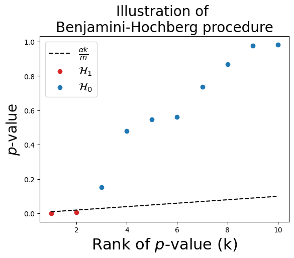
Figure 1: Illustration of the Benjamini-Hochberg procedure. $p$-values are sorted by increasing order. The threshold is the greatest $p$-value that is lower than $\alpha k/m$, when $k$ is the rank of the $p$-value.

The striking property of this procedure is to yield the desired control of the FDR at the prescribed level $\alpha$ as stated by the next result.

Theorem 1 (FDR control with BH [5]).

Let $m$ be a positive integer and $(X_{i})_{1}^{m}$ be independent random variables such that $X_{i}\sim\mathcal{P}_{0}$, $1\leq i\leq m_{0}$, and $X_{i}\sim\mathcal{P}_{1}$, $m_{0}+1\leq i\leq m$. Let us also define the set of true $p$-values, for all $1\leq i\leq m$ by $p_{i}=\mathbb{P}_{X\sim P_{0}}(X\geq X_{i})\in[0,1]$, and assume that each $p_{i}\sim U([0,1])$. Then for every $\alpha\in]0,1]$, $BH_{\alpha}$ applied to $p=(p_{i})_{1\leq i\leq m}$ yields the exact FDR control at the prescribed level $\alpha$ that is,

$$FDR_{1}^{m}(\varepsilon_{BH_{\alpha}},p)=\frac{m_{0}\alpha}{m}.$$

The proof of the theorem is deferred to Appendix A.3. In particular, the FDR control results from the fact that under $\mathcal{H}_{0}$, the true $p$-values follow a uniform distribution. The equality could be replaced by an upper bound if the uniform distribution assumption were weakened by the super-uniform property.

By contrast with the previous framework, when performing anomaly detection, the abnormality score is computed using a scoring function (Definition 1), and the true $p$-value is given by

$$p_{t}=\mathbb{P}_{X\sim\mathcal{P}_{0}}\left(a(X)\geq a(X_{t})\right),$$

where the notation clearly emphasizes the dependence with respect to the unknown reference distribution. This justifies why empirical $p$-values are now substituted to true ones as earlier explained (see Eq. 2.4).

A difficulty resulting from using empirical $p$-values in the BH-procedure is that the FDR control does no longer hold true as illustrated by Figure 2. This figure displays the actual FDR value (plain blue curve) versus the cardinality of the calibration set used to computed the empirical $p$-values (see Definition 2) in the specific situation of Gaussian data. Except for some a few values of the calibration set cardinality, the FDR control is no longer achieved (red horizontal line). Furthermore the actual FDR value is higher than the desired $m_{0}/m\alpha$. This results from the fact that the super uniform property is violated when using empirical $p$-values as established by Proposition 1 below.

Proposition 1 (Distribution of empirical $p$-value under $H_{0}$).

Let $X\sim\mathcal{P}_{0}$ where $\mathcal{P}_{0}$ is the probability distribution under $\mathcal{H}_{0}$, the calibration set cardinality is denoted by $n$, and $\{X_{1},\dots,X_{n}\}\sim\mathcal{P}_{0}^{n}$ is the calibration set. If one further assumes that there are no ties among $a(X_{1}),\ldots,a(X_{n})$, then the empirical $p$-value at $X$ is denoted by $\hat{p}\mbox{-value}(X;\{X_{1},\ldots,X_{n}\})$ and follows the discrete uniform distribution

$$U(0,\frac{1}{n},\frac{2}{n},\ldots,1).$$

Let us mention that under $\mathcal{H}_{0}$ the empirical $p$-value has a different distribution from that of the conformal $p$-value [41] which follows $U(1/(n+1),\ldots,1)$. The conformal $p$-value is never smaller than $1/(n+1)$, which raises issues in terms of the detection power with lots of false negatives (see the right panel of Figure 11 and the discussion in Appendix A.1). With empirical $p$-values, it can be easily checked that

$$\mathbb{P}\left(\hat{p}\mbox{-value}(X;\{X_{1},\ldots,X_{n}\})\leq 0\right)=\frac{1}{n+1}>0,$$

which violates the super uniformity property. As a consequence, FDR is no longer controlled by the BH-procedure [6] applied to empirical $p$-values. Other consequences owing to the use of empirical $p$-values violating super uniformity are illustrated in Section 3.1.

The assumption of no ties are allowed among the scores $a(X_{i})$s is quite mild and fulfilled most of the time as supported by Example Examples as long as the reference distribution is continuous (admits a density).

Proof of Proposition 1.

Since $X\sim\mathcal{P}_{0}$ and $X_{1},\ldots,X_{n}\sim\mathcal{P}_{0}^{n}$ are independent, the empirical $p$-value $\hat{p}$ is a random variable computed from $X$ and $X_{1}^{n}$ and satisfies for any $0\leq\ell\leq n$ that

$$\mathbb{P}(\hat{p}=\ell/n)$$

$$=\mathbb{P}(a(X_{(\ell+1)})<a(X)\leq a(X_{(\ell)}))$$

$$=\mathbb{P}(\{\mbox{rank of $a(X)$ among $\{a(X),a(X_{1}),\ldots,a(X_{n})\}$ is $\ell+1$}\}),$$

where $a(X_{(n)})<a(X_{(n-1)})<\cdots<a(X_{(1)})$. The conclusion comes from noticing that the probability distribution of $\{X,X_{1},\ldots,X_{n}\}$ is exchangeable, and assumption of no ties in scores $a(X_{i})$ ∎

Let us also notice that Figure 2 shows that there exist particular values of the calibration set cardinality for which FDR is still controlled at the prescribed level. This perspective is further explored in Section 3.2.2, where a new multiple testing procedure yielding the desired FDR control for the whole time series is devised.

3 FDR control with Empirical $p$-values

The goal here is to describe a strategy achieving the desired FDR control for a time series of length $m$ when using empirical $p$-values. A motivating example is first introduced for emphasizing the issue in Section 3.1. Then a theoretical understanding is provided along Section 3.2 which results in a new solution which applies to independent empirical $p$-values. An extension is then discussed to the non-independent setup in Section 3.3.1. Finally experimental results are reported in Section 3.4 to (empirically) assess the validity of our previous theoretical conclusions.

3.1 Motivating example

The purpose here is to further explore the effect of the calibration set cardinality on the actual FDR control when using empirical $p$-values. This gives us more insight on how to find mathematical solutions.

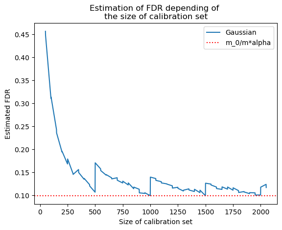
Figure 2:

Let us start by generating observations using two distributions. The reference distribution is $\mathcal{P}_{0}=\mathcal{N}(0,1)$ and the alternative distribution is $\mathcal{P}_{1}=\mathcal{N}(4,10^{-4})$. The anomalies are located in the right tail of the reference distribution. The length $m$ of the signal is $m=100$. The number of observations under $\mathcal{P}_{0}$ is $m_{0}=99$. The experiments have been repeated $K=10^{4}$ times.

Figure 2 displays the actual value of FDR as a function of the cardinality $n$ of the calibration set $\{x_{1},...,x_{n}\}$ used to compute the empirical $p$-values (see Definition 2). One clearly see that FDR is not uniformly controlled at level $m_{0}/m\alpha$. However there exist particular values of $n$ for which this level of control is nevertheless achieved. As long as $n$ has become large enough ($n\geq 500$), repeated picks can be observed with a decreasing height as $n$ grows.

3.2 FDR control: main results for i.i.d. $p$-values

The present section aims at first explaining the shape of the curve displayed in Figure 2. This will help getting some intuition about how to design an online procedure achieving the desired FDR control for the full time series.

3.2.1 Proof of FDR control by BH revisited

The main focus is now given to independent $p$-values. In what follows, the classical proof (Proof A.3) of the FDR control by the BH-procedure is revisited then leading to the next result. Its main merit is to provide the mathematical expression of the plain blue curve observed in Figure 2.

Theorem 2.

Let $n$ be the cardinality of the calibration set and $m$ be that of the set of tested hypotheses where $\{X_{1},\ldots,X_{m}\}$ denotes a set of random variables. Let $m_{0}\leq m$ be the cardinality of the random variables from the reference distribution $\mathcal{P}_{0}$. Let the empirical $p$-value be denoted, for any $i\in\llbracket 1,m\rrbracket$, by $\hat{p}_{i}=\hat{p}\mbox{-value}(X_{i},\{Z_{i,1},\ldots,Z_{i,n}\})$, where the calibration set is $\{Z_{i,1},\ldots,Z_{i,n}\}$ and each $Z_{i,j}\sim\mathcal{P}_{0}$. Let the random variables $R(i)$ be the number of detections raised by $BH_{\alpha}$ when replacing $X_{i}$ with 0, as defined along the proof detailed in Appendix A.3. Then for every $\alpha\in]0,1]$, the FDR value over the sequence from 1 to $m$ is given by

$$FDR_{1}^{m}(\hat{\varepsilon}_{{BH}_{\alpha}},\hat{p})=m_{0}\sum_{k=1}^{m}\frac{\frac{\lfloor\frac{\alpha kn}{m}\rfloor+1}{n+1}}{k}\mathbb{P}(R(i)=k),$$

where $\hat{\varepsilon}_{{BH}_{\alpha}}$ denotes the $BH_{\alpha}$ threshold from Definition 3 when the BH-procedure is applied to the empirical $p$-values $\hat{p}=(\hat{p}_{i};1\leq i\leq m)$.

In general it is not possible to compute the exact value of the $FDR$ without knowing the distribution of the random variables $R(i)$. This is in contrast with the case of true $p$-values where $\mathbb{P}(p_{i}\leq\frac{\alpha k}{m})=\frac{\alpha k}{m}$, whereas with empirical $p$-values $\mathbb{P}(\hat{p}_{i}\leq\frac{\alpha k}{m})=\frac{\lfloor\frac{\alpha kn}{m}\rfloor+1}{n+1}$, which prevents from any simplification of the final bound. Nevertheless this value still suggests a solution to circumvent this difficulty: requiring conditions on $\alpha$, $m$, and $n$ such that $\frac{\lfloor\frac{\alpha kn}{m}\rfloor+1}{n+1}=\frac{\alpha k}{m}$, for all $k$. This is precisely the purpose of next Corollary 1.

Proof of Theorem 2.

When applying Proof A.3, the only modification is that $\mathbb{P}(\hat{p}_{i}\leq\frac{\alpha k}{m})$ is not equal to $\frac{\alpha k}{m}$ since $\hat{p}_{i}$ now follows the discrete uniform distribution

$$\mathbb{P}(\hat{p}_{i}\leq\frac{\alpha k}{m})=\sum_{\ell=0}^{\lfloor n\alpha k/m\rfloor}\mathbb{P}(n\hat{p}_{i}=\ell)=\frac{\lfloor\frac{\alpha kn}{m}\rfloor+1}{n+1}.$$

Plugging this in the FDR expression, it gives

$$FDR_{1}^{m}(\hat{\varepsilon}_{{BH}_{\alpha}},\hat{p})=m_{0}\sum_{k=1}^{m}\frac{\frac{\lfloor\frac{\alpha kn}{m}\rfloor+1}{n+1}}{k}\mathbb{P}(R(i)=k).$$

Recall that $\hat{p}_{i}$ follows $U(0,1/n,2/n,\ldots,1)$ entails that $n\hat{p}_{i}$ follows $U(0,1,2,\ldots,n)$. ∎

3.2.2 Tuning of the calibration set cardinality

Corollary 1.

Under the same notations and assumptions as Theorem 2, the next two results hold true.

1. Assume that there exists an integer $1\leq\ell$ such that $\frac{\ell m}{\alpha}$ is an integer. If the cardinality $n$ of the calibration set satisfies $n=n_{\ell}-1=\ell m/\alpha-1$, then

   $$FDR_{1}^{m}(\hat{\varepsilon}_{{BH}_{\alpha}},\hat{p})=\frac{m_{0}\alpha}{m}.$$

2. For every $\alpha\in]0,1]$, assume that the cardinality of the calibration set satisfies $n=n_{\ell}-1=\lceil\frac{\ell m}{\alpha}\rceil-1$, for any integer $\ell\geq 1$. Then,

   $$\frac{n}{(n+1)}\frac{m_{0}\alpha}{m}\leq FDR_{1}^{m}(\hat{\varepsilon}_{{BH}_{\alpha}},\hat{p})\leq\frac{m_{0}\alpha}{m}.$$

The proof is postponed to Section A.4. The first statement in Corollary 1 establishes that recovering the desired control of FDR at the exact prescribed level $\alpha$ is possible on condition that the calibration set cardinality is large enough and more precisely that $n=\ell m/\alpha-1$. This (mild) restriction on the values of $\alpha$ reflects that the empirical $p$-values do not satisfy the super-uniformity property. By contrast, the second statement yields the desired control at the level $\alpha m_{0}/m$ by means of lower and upper bounds. In particular, the lower bound tells us that the FDR value can be not lower than the desired level $\alpha m_{0}/m$ up to a multiplicative factor equal to $1-1/n$, which goes 1 as $n$ grows. For instance with $\alpha=0.1$ and $m=100$, $n_{\ell}=1000$ would yield that $FDR_{1}^{m}(\hat{\varepsilon}_{{BH}_{\alpha}},\hat{p})\cdot m/(m_{0}\alpha)\in[0.999,1]$. This small lack of control is the price to pay for allowing any value of $\alpha\in]0,1]$. It is also important to recall that in the anomaly detection field, abnormal events are expected to be rare. As a consequence $\frac{m_{0}}{m}$ is close to $1$ and the actual $FDR$ level is close to the desired $\alpha$. However in situations where $m_{0}/m$ could depart from 1 too strongly, then incorporating an estimator of $m_{0}/m$ would be helpful.

3.3 Extension to dependent $p$-values

In Section 3.2, Corollary 1 states that FDR is controlled at a prescribed level with empirical $p$-values for which the super-uniformity property is not fulfilled. A key ingredient in the proof was the independence property across empirical $p$-values. One purpose of the present section is to extend these results to non-independent $p$-values.

Towards this extension, the concept of positive regression dependency (referred to as PRDS) [6] turns out to be useful. The PRDS property is a form of positive dependence between $p$-values where all pairwise $p$-value correlations are positive. It results that a small $p$-value for a given observation makes other $p$-values for all considered observations simultaneously small as well, and vice-versa [4].

3.3.1 Theoretical results to dependent $p$-values

A classical result established in [6] proves that FDR is upper bounded by $\alpha m_{0}/m$ provided the $p$-value family satisfies the PRDS and super-uniformity properties. It turns out that this result can be extended to our estimator with the same choice of calibration set cardinality as the one discussed in Corollary 1. Another important achievement is the fact that FDR can be also lower bounded in the case where the calibration set is the same for all (empirical) $p$-values (see Definition 2). This results originally proved by [41] is extended here to empirical $p$-values computed with a calibration set cardinality tuned as suggested in Corollary 1.

In Section 3.2, considering the size of the calibration set is correctly chosen, it has been proved that the control of the FDR can be achieved with estimated $p$-values for which the super-uniformity property is not fulfilled. The results obtained for i.I.d. $p$-values will be extended in this section for non i.i.d. $p$-values.

For this extension, the concept of positive regression dependency on each one from a subset called PRDS [6] is introduced. The PRDS property is a form of positive dependence of $p$-values where all pairwise $p$-value correlations are positive. Larger scores in the calibration set make the $p$-values for all test points simultaneously smaller, and vice-versa [4].

Definition 1 (PRDS property).

A family of $p$-values $\hat{p}_{1}^{m}$ is PRDS on a set $I_{0}\subset\{1,\ldots,m\}$ if for any $i\in I_{0}$ and any increasing set $A$, the probability $\mathbb{P}[\hat{p}_{1}^{m}\in A|\hat{p}_{i}=u]$ is increasing in $u$.

A classical result in [6] asserts that the FDR is upper bounded by $\frac{m_{0}}{m}\alpha$ in the case where the $p$-value family is PRDS and super-uniform. This result can be extended our estimator with the same choice of calibration set cardinality than in Theorem 1.

Corollary 2 (Corollary of Theorem 1.2 in [6]).

Suppose the family of $p$-values $\hat{p}_{1}^{m}$ is PRDS on the set $\mathcal{H}_{0}$ of true null hypotheses and suppose that $\hat{p}_{1}^{m}$ respects super-uniformity an all thresholds that can may resulting from BH

$$\forall k\in\llbracket 1,m\rrbracket\qquad\mathbb{P}(\hat{p}_{i}<\frac{\alpha k}{m})\leq\frac{\alpha k}{m},$$

Then, the $FDR$ is upper-bounded by $\alpha$

$$FDR(\hat{p},\hat{\varepsilon}_{B}H)\leq\frac{m_{0}\alpha}{m}$$

Unique calibration set

More over, in the case where the calibration set is the same for all $p$-values, the FDR can also be lower bounded as shown in [41]. This result can be extended to empirical $p$-values given in Definition 2 with a calibration set cardinality tuned as proposed in Theorem 1.

Corollary 3 (Corollary of Theorem 3.4 in [41]).

Assuming the following conditions: Let $n$ be the cardinality of the calibration set, $m$ be the cardinality of the active set and $m_{0}$ the number of normal observations. Let $\mathcal{P}_{0}$ be the reference distribution. Let $Z_{i}$ for $i$ in $\llbracket 1,m\rrbracket$ independents random variables, following $\mathcal{P}_{0}$. Let $X_{i}$ for $i$ in $\llbracket 1,m\rrbracket$ be random independents variables and independents from $(Z_{j})$. There are exactly $m_{0}$ random variables following the $\mathcal{P}_{0}$ distribution. Let $a$ be a scoring function. For all $i$ in $\llbracket 1,m\rrbracket$, let $\hat{p}_{i}$ be the empirical $p$-values associated with the random variables $X_{i}$ and computed as follows, $\hat{p}_{i}=p\mbox{-value}(X_{i},\{Z_{1},...,Z_{m}\},a)$.

If the cardinality of the calibration set is a multiple of $n=n_{\ell}=\ell m/\alpha-1$, then the FDR using $\hat{BH}_{\alpha}$ on $(\hat{p}_{i})_{1\leq i\leq m}$ is equal to $\frac{m_{0}\alpha}{m}$:

$$FDR_{1}^{m}(\hat{\varepsilon}_{{BH}_{\alpha}},\hat{p})=\frac{m_{0}\alpha}{m}$$

Overlapping calibration set

In the context of online anomaly detection, moving windows are classically used to capture and process the incoming data. This is why the calibration sets of the $p$-value family will overlap. To have a perfect control of the FDR, an upper and lower bounds is needed.

According Proposition 2, $p$-values with overlapping calibration sets are PRDS.

Proposition 2 (PRDS property for overlapping calibration sets).

Let $X_{i}$ for $i$ in $\llbracket 1,m\rrbracket$ be random independents variables. There are exactly $m_{0}$ random variables following the $\mathcal{P}_{0}$ distribution, with belong to $\mathcal{H}_{0}$. Let Z be the random vector that combine all calibration set, all elements of Z are generated from $\mathcal{P}_{0}$. The set of $n$ indices defining the elements of calibration set related to $\hat{p}_{i}$ in Z is noted $\mathcal{D}_{i}$. The calibration set related to $X_{1}$ is noted $\textbf{Z}_{\mathcal{D}_{1}}=(\textbf{Z}_{i_{1}},...,\textbf{Z}_{i_{n}})$. For all $i$ in $\llbracket 1,m\rrbracket$: $\hat{p}_{i}=p\mbox{-value}(X_{i},\textbf{Z}_{\mathcal{D}_{i}})$.

Under these conditions, the set of $p$-values is PRDS on $\mathcal{H}_{0}$

The proof of the proposition is in delayed to Appendix A.2. Since such $p$-values are are PRDS, it gives an upper bound control of the FDR using Corollary 4.

Corollary 4 (PRDS property for overlapping calibration sets).

Under the same conditions as Proposition 2 and the condition on calibration set cardinality satisfy $\exists\ell\geq 1,n=\ell\frac{m}{\alpha}-1$:

$$FDR(\hat{p},\hat{\varepsilon}_{BH})\leq\frac{m_{0}\alpha}{m}$$

3.3.2 Calibration set and impact of the overlap

In the context of online anomaly detection, moving windows are usually used to capture and process the incoming observations. In this context, the calibration set coincides with the observations within this window. Since successive windows are overlapping each other depending on the size of the shift, the resulting calibration sets used for computing the successive empirical $p$-values are also overlapping. To have a perfect control of the FDR, an upper and lower bounds are needed. Since the Appendix A.2 proves that such $p$-values are PRDS, it gives an upper bound control of the FDR. No theoretical results exists to compute the lower bound, indeed the existing proof in [41] did not extend to overlapping calibration sets. Therefore the next discussion suggests to establish this lower bound empirically.

The following experiments aims at drawing a comparison between the FDR values in three scenarios: independent calibration sets, partially overlapping calibration sets with an overlap size driven by the value of $sn$ (size of the shift), and the same calibration set for all empirical $p$-values. To be more specific, the calibration sets (and corresponding empirical $p$-values) were generated according to the following scheme. Each calibration set is of cardinality $n$. When moving from one calibration set to the next one, the shift size is equal to $sn$, where $s$ in $[0,1]$ is the proportion of independent data between calibration sets, resulting in an overlap of cardinality $(1-s)n$. Therefore an overlap occurs as long as $s<1$. All these ways to build the calibration sets are called “calibration sets strategies”.

1. The independent $p$-values (iid Cal.) are generated according to

   $$\forall i\in\llbracket 1,m\rrbracket,\quad\textbf{Z}_{i}\sim\mathcal{P}_{0}^{n},\quad\hat{p}_{1,i}=\hat{p}\mbox{-value}(X_{i},\textbf{Z}_{i}).$$ (3.1)

2. The $p$-values with the same calibration set (Same Cal.) are generated by

   $$\forall i\in\llbracket 1,m\rrbracket,\quad\textbf{Z}\sim\mathcal{P}_{0}^{n},\quad\hat{p}_{2,i}=\hat{p}\mbox{-value}(X_{i},\textbf{Z}).$$ (3.2)

3. The $p$-values with overlapping calibration sets (Over. Cal.) are generated given, for $0<s<n$, by

   $$\forall i\in\llbracket 1,m\rrbracket,\quad\textbf{Z}_{i} =\{Z_{\lfloor isn\rfloor+1},\ldots,Z_{\lfloor isn\rfloor+n}\},\quad\hat{p}_{3,i}=\hat{p}\mbox{-value}(X_{i},\textbf{Z}_{i}),$$

   and $$\{Z_{s+1},\ldots,Z_{\lfloor 2sn\rfloor+1},\ldots,Z_{\lfloor msn\rfloor+1},\ldots,Z_{\lfloor msn\rfloor+n}\}\sim\mathcal{P}_{0}^{ms+n}.$$ (3.3)

According to these three scenarios, as $s$ increases, the overlap cardinality decreases, which results in more and more (almost) independent calibration sets. This is illustrated by the empirical results collected in Table 1. For each calibration set strategy, presented in row, and for each calibration set cardinality in column, the estimated FDR is shown. In this experiment, the reference distribution $\mathcal{P}_{0}$ is the Gaussian $\mathcal{N}(0,1)$ and the anomalies are equal to $\Delta=4$. The number of tested $p$-values, noted $m$, is equal to $100$ and $m_{1}$, the number of anomalies, is equal to $1$. On each sample, BH-procedure is applied with $\alpha=0.1$ and the $FDP$ is computed. Each FDR is estimated over $10^{3}$ repetitions.

Table 1: FDR results with overlapping calibration sets

n	249	250	499	500	749	750	999	1000
Same Cal.	0.164	0.175	0.112	0.183	0.137	0.131	0.097	0.154
Over Cal. (s=0.1%)	0.167	0.174	0.100	0.156	0.138	0.125	0.093	0.140
Over Cal. (s=0.2%)	0.162	0.176	0.095	0.170	0.124	0.127	0.109	0.143
Over Cal. (s=0.5%)	0.163	0.166	0.110	0.170	0.116	0.132	0.111	0.149
Over Cal. (s=1%)	0.151	0.180	0.094	0.177	0.127	0.128	0.099	0.143
Over Cal. (s=2%)	0.164	0.180	0.108	0.179	0.133	0.140	0.097	0.143
Over Cal. (s=5%)	0.168	0.172	0.108	0.169	0.125	0.130	0.096	0.144
Over Cal. (s=10%)	0.165	0.181	0.104	0.185	0.122	0.140	0.105	0.146
Over Cal. (s=20%)	0.173	0.207	0.109	0.171	0.136	0.149	0.101	0.140
Over Cal. (s=50%)	0.180	0.187	0.103	0.183	0.121	0.128	0.094	0.143
iid Cal.	0.171	0.188	0.115	0.174	0.138	0.143	0.104	0.132

The values of $n$ in the columns of Table 1 are chosen such that, for each pair of columns, the FDR value is smaller for the left column and larger for the right column (see Figure 2 for a visual illustration of this phenomenon). Table 1 illustrates that, in the context of the present numerical experiments, the FDR estimation is not too strongly impacted by the value of $s$ (proportion of the overlap). To assert that the observed differences between FDR estimations in each column are not significant, permutation tests [16, 47] are performed. Under $\mathcal{H}_{0n}$ hypothesis, the $FDR$ are the same across all calibration set strategies for the calibration set cardinality $n$. Under $\mathcal{H}_{1n}$ there are at least two calibration strategies leading to different $FDR$. The $FDP$ samples that have been used to estimate the $FDR$ are reused. The maximal gap between sample means is used as statistic. The test is performed using the function “permutation_test” from the Python library called Scipy. The significance level is fixed at $0.05$. Since multiple tests are performed over the different cardinalities, the threshold for rejecting a hypothesis is $0.00625$, according Bonferroni correction. The results are display in Table 2. All tested hypotheses have a $p$-values greater than the threshold $0.00625$. There are no significant difference in the resulting FDR between the different proportions of overlapping in calibration sets. This would suggest that considering overlapping calibration sets should not worsen too much the control of false positives and negatives.

Table 2: $p$-values resulting from permutations test

n	249	250	499	500	749	750	999	1000
$p$-value of the test	0.300	0.0326	0.572	0.313	0.588	0.435	0.735	0.690

3.4 Empirical Results: Assessing the FDR control

The purpose of the present section is to compute the actual FDR value when empirical $p$-value are used instead of true ones. The question raised here is to check whether the FDR of the full time series is truly controlled at a prescribed level $\alpha$. The empirical results must be compared with the theoretical FDR expression that has been established in Theorem 2.

In what follows, Section 3.4.1 describes the simulation design that has been considered, Section 3.4.2 details the criteria used for the assessment, and Section 3.4.3 discusses the experimental results.

3.4.1 Simulation design

Two scenarios have been considered to explore how much the thickness of the distribution tails can influence the results.

1. Thin tails:

   The reference probability distribution is $\mathcal{P}_{0}=\mathcal{N}(0,1)$ for normal observations and $\mathcal{P}_{1}=\delta_{\Delta_{\mathcal{N}}}$ for anomalies, where $\Delta_{\mathcal{N}}\in\mathbb{R}$ is a parameter encoding the strength of the shift. Here $\delta_{\Delta_{\mathcal{N}}}$ denotes the Dirac measure such that $\delta_{\Delta_{\mathcal{N}}}(z)=1$ if $z=\Delta_{\mathcal{N}}$ and 0 otherwise. A Gaussian reference distribution and anomalies generated from a Dirac distribution in the right tail. $\Delta_{\mathcal{N}}$ is the size of the abnormal spike in the Gaussian distribution.

2. Thick tails:

   $\mathcal{P}_{0}=\mathcal{T}(5)$ is a Student probability distribution with 5 degrees of freedom and $\mathcal{P}_{1}=\delta_{\Delta_{\mathcal{T}}}$ denotes the alternative distribution of anomalies, where $\Delta_{\mathcal{N}}\in\mathbb{R}$ is a parameter encoding the strength of the shift.

Regarding the value of the shift strength in Scenarios 1 and 2, two values of $\Delta_{\mathcal{N}}$ have been considered $3.5$ and $4$. The values of $\Delta_{\mathcal{T}}$ have been chosen such that

$$\mathbb{P}_{X\sim\mathcal{N}(0,1)}(X>\Delta_{\mathcal{N}})=\mathbb{P}_{X\sim\mathcal{T}(5)}(X>\Delta_{t})$$

for each choice of $\Delta_{\mathcal{N}}$. This avoids any bias in the comparison of the detection power of the considered strategy depending on the ongoing scenario.

Different cardinalities have been considered for the calibration set following the mathematical expression

$$n\in\{k\cdot 10,k\in\llbracket 1,200\rrbracket\}\cup\{\ell\cdot 10-1,\ell\in\llbracket 1,200\rrbracket\}.$$

In particular all integers between 10 and 2 000 are explored with a step size equal to 10 as well as all integers between 9 and 1 999 with a step size of 10. This choice is justified by the particular expression of the FDR value provided by Theorem 2.

All the $n$ elements of the calibration set are generated from the reference distribution that is, $\{Z_{1},\dots,Z_{n}\}\sim\mathcal{P}_{0}$. All the $m$ observations corresponding to the tested hypotheses $\{X_{1},\dots,X_{m}\}$ are generated according to a mixture of $m_{1}=1$ anomalies from $\mathcal{P}_{1}$ and $m_{0}=m-m_{1}$ normal observations from $\mathcal{P}_{0}$. Here $m=100$ and $m_{0}=99$.

Each simulation condition has been repeated $B=10^{4}$ times. For each repetition $1\leq b\leq B$, the observations are indexed by $b$ such that $X_{b,j}\sim\mathcal{P}_{1}$ for each $j\in\llbracket 1,m_{1}\rrbracket$, and $X_{b,j}\sim\mathcal{P}_{0}$ for $j\in\llbracket m_{1}+1,m\rrbracket$.

3.4.2 Criteria for the performance assessment

In the present scenarios, anomalies are all located in the right tail of the reference probability distribution. Therefore the empirical $p$-value are computed according to Definition 2 with the scoring function $a(x)=x$. For each repetition $1\leq b\leq B$,

$$\forall 1\leq j\leq m,\quad\hat{p}_{b,j}=p\mbox{-value}(X_{b,j},\{Z_{b,1},\dots,Z_{b,n}\}).$$

After computing the empirical $p$-values, the $BH_{\alpha}$ procedure (see Definition 3) is applied in such a way that, for any $1\leq j\leq m$,

$$d_{b,j}=\mathds{1}_{BH_{\alpha}(\hat{p}_{b,1},\dots,\hat{p}_{b,m})}(j),$$

where $\mathds{1}_{I}$ denotes the indicator function of the index set $I$. The FDP value of the sequence from 1 to $m$ is computed from the knowledge of the true label of the observations as “normal” or “anomaly”. For each repetition $1\leq b\leq B$,

$$(FDP_{1}^{m})_{b}=\frac{\sum_{j=m_{1}+1}^{m}d_{b,j}}{\sum_{j=1}^{m}d_{b,j}}.$$

The results obtained after the $B$ repetitions are averaged within the FDR estimate of the sequence from 1 to $m$ as

$$FDR_{1}^{m}=\frac{1}{B}\sum_{b=1}^{B}(FDP_{1}^{m})_{b}.$$

The FNR value of the sequence from 1 to $m$ (Equation 2.2) is estimated by

$$(FNP_{1}^{m})_{b}=\frac{1}{m-m_{0}}\sum_{j=m_{0}+1}^{m}d_{b,j},\quad\mbox{and}\quad FNR_{1}^{m}=\frac{1}{B}\sum_{b=1}^{B}(FNP_{1}^{m})_{b}.$$

3.4.3 Experimental discoveries

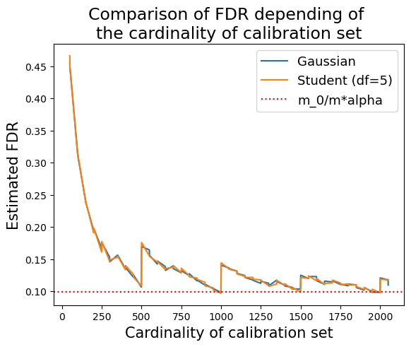
(a) FDR depending on $n$ with 4 sigmas anomalies

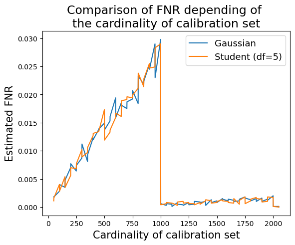
(b) FNR depending on $n$ with 4 sigmas anomalies

(c) FDR depending on $n$ with 3.5 sigmas anomalies

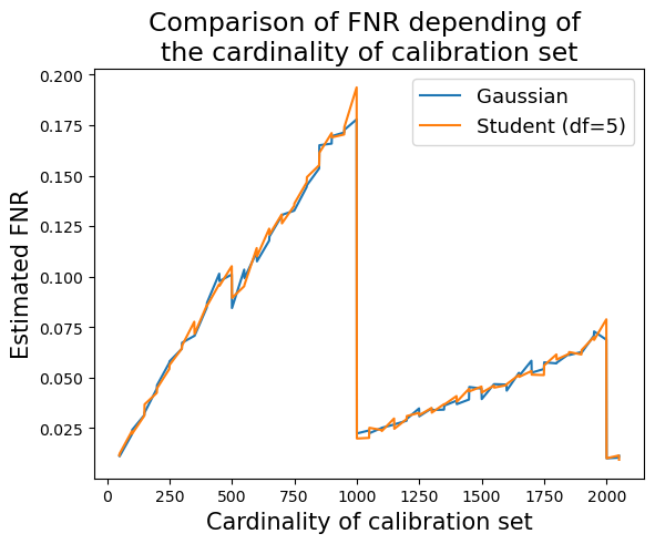
(d) FNR depending on $n$ with 3.5 sigmas anomalies

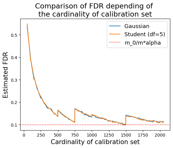
(e) FDR depending on $n$ with 4 sigmas anomalies and $m=150$

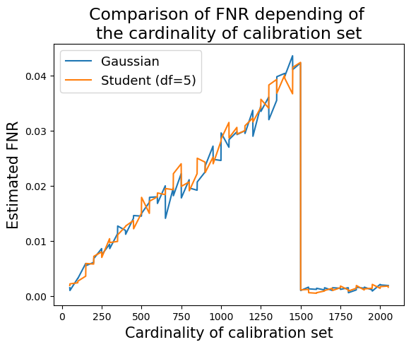
(f) FNR depending on $n$ with 4 sigmas anomalies and $m=150$

Figure 3: Effect of calibration set cardinality and abnormality score on the FDR control and the FNR

Figure 3 displays the FDR value (left panel) and the FNR value (right panel) as a function of the calibration set cardinality for the two scenarios (Gaussian and Student) described in Section 3.4.1. The blue (respectively orange) curve corresponds to the Gaussian (resp. Student) reference distribution. The horizontal line is the prescribed level $\alpha=0.1$ at which FDR should be controlled with true $p$-values (Theorem 1). Figures 3(a) and 3(b) are obtained with $\Delta_{\mathcal{N}}=4$, while Figures 3(c) and 3(d) result from $\Delta_{\mathcal{N}}=3.5$.

According to these plots, the behavior of both FDR and FNR does not exhibit any strong dependence with respect to the reference probability distribution. The results are very close for both Gaussian and Student distributions.

As illustrated by Figures 3(a) and 3(c), the FDR control at the prescribed level is achieved for particular values of the calibration set cardinality. These values coincide with the ones exhibited by Theorem 1, which are multiples of $\alpha/m=10^{3}$ (up to a downward shift by 1).

A striking remark is that the FNR curve sharply increases from 1 to $n=999$. This reflects that although the FDR value becomes (close to) optimal as $n$ increases from 1 to $n=999$, the proportion of false negatives simultaneously increases leading to a suboptimal statistical performance (because of too many false negatives). Fortunately a larger cardinality $n$ of the calibration set, for instance $n=1999$, would greatly improve the results at the price of a larger calibration set, which also increases the computational cost.

Consistently with what is established in Theorem 1, the FDR value does not depend on the strength of the distribution shift $\Delta$ as illustrated by Figures 3(a) and 3(c). As long as FDR is concerned (which is an expectation), the shift plays no role. Let us mention that focusing of the expectation does not say anything about the probability distribution of FDP, which can be influenced by the shift strength. By contrast, the comparison of Figures 3(b) and 3(d) clearly shows the impact of the shift strength on the FNR value. As the shift strength becomes lower, anomalies are more difficult to be detected which inflates the FNR value.

The best cardinality $n$ of the calibration set depends on the number $m$ of tested hypotheses according to Theorem 1. For instance, Figure 3(a) shows the value $n=999=100/0.1-1$ as a good candidate since it achieves the desired FDR control while reducing both the number of false negatives and the computation cost. By contrast, Figure 3(e) rather exhibits the value $n=1499=150/0.1-1$ as the smallest $n$ allowing a perfect FDR control and a small number of false negatives.

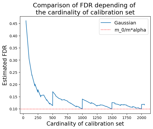
(a) $m_{1}=1$

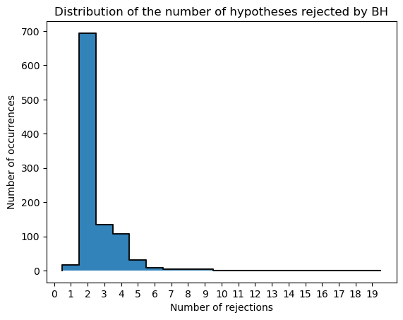
(b) $m_{1}=1$

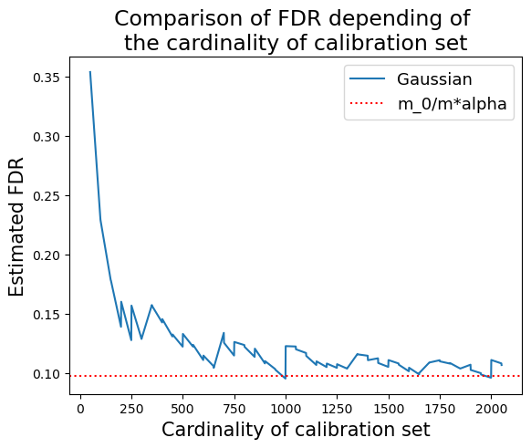
(c) $m_{1}=2$

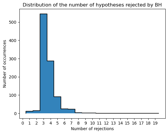
(d) $m_{1}=2$

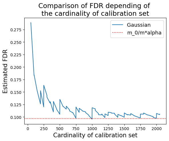
(e) $m_{1}=3$

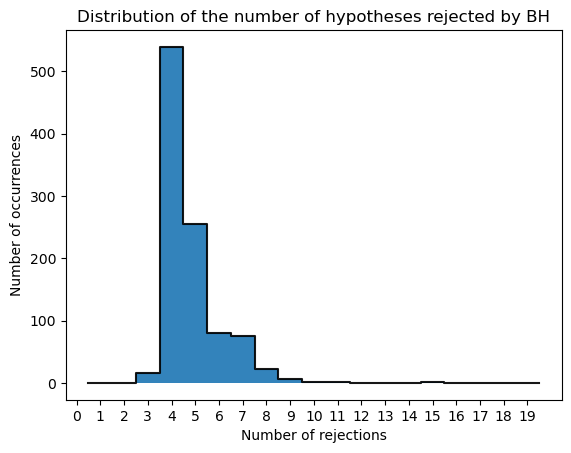
(f) $m_{1}=3$

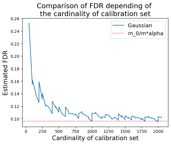
(g) $m_{1}=4$

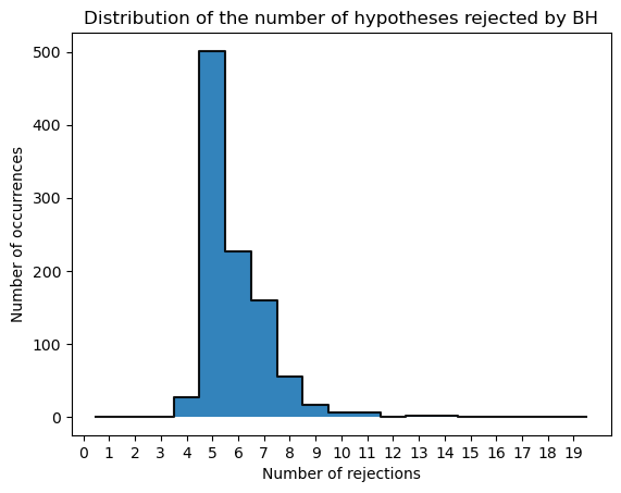
(h) $m_{1}=4$

Figure 12: Effect of the number detections by BH on the intermediate drops for the FDR control

Figure 3(a) shows other intermediate values calibration set cardinalities yielding the FDR control. For instance $n=1499$ (between $n=999$ and $n=1999$) is predicted by Theorem 1. However complementary experiments (summarized by Figure 12 in Appendix B.1) illustrate that these intermediate values of $n$ allowing the FDR control actually depend on the number of anomalies $m_{1}$. Their existence can be explained by the distribution of the number of detections. For example, Figure 12(d) shows a high probability of detecting $3$ anomalies. Assuming there exists $k^{*}\in\llbracket 1,m\rrbracket$ such that $\mathbb{P}(R(i)=k^{*})\approx 1$, Theorem 2 justifies that

$$FDR_{1}^{m}(\hat{\varepsilon}_{BH_{\alpha}},\hat{p}) =\frac{n}{n+1}\cdot\alpha\frac{m_{0}}{m}+\frac{m_{0}}{n+1}\sum_{k=1}^{m}\frac{(1-q_{n,k})}{k}\mathbb{P}(R(i)=k)$$

$$\approx\frac{n}{n+1}\cdot\alpha\frac{m_{0}}{m}+\frac{m_{0}}{n+1}\frac{(1-q_{n,k^{*}})}{k^{*}}.$$

Then the proof detailed in Appendix A.4 yields that $1-q_{n,k^{*}}=\frac{\alpha}{m(n+1)}$ can be reached for all $\ell\geq 1$, such that $n=\ell\frac{m}{\alpha k^{*}}-1$. This allows to conclude that $FDR_{1}^{m}(\hat{\varepsilon}_{BH_{\alpha}},\hat{p})\approx\frac{m_{0}\alpha}{m}$.

3.4.4 How to choose the right cardinality of the calibration set?

Intuitively an optimal choice of the cardinality $n$ of the calibration set should enable the FDR control while minimizing the number of false negatives and avoiding any excessive computation time. To achieve this objective, the first part of Corollary 1 explains that $n$ must be chosen from the set $\mathcal{N}=\{\ell m/\alpha-1,\quad\ell\geq 1\}$. Using the simulation scenarios described in Section 3.4.1, the aim is to visualize the relationship between the calibration set cardinality and FNR when $n\in\mathcal{N}$. The results are summarized by Figure 4 where the FNR value is displayed versus $n$.

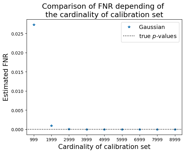
(a) $\Delta=4$, $m_{1}=1$

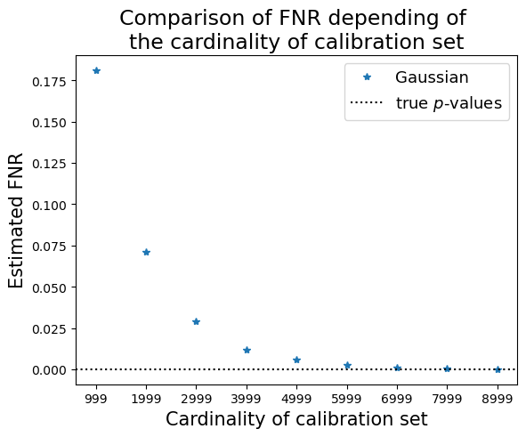
(b) $\Delta=3.5$, $m_{1}=1$

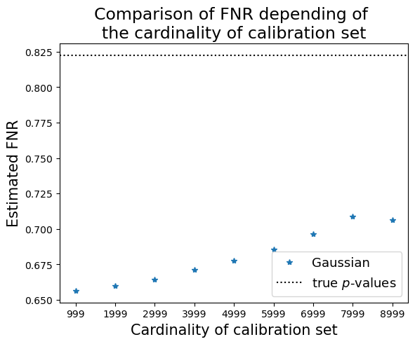
(c) $\Delta=3$, $m_{1}=1$

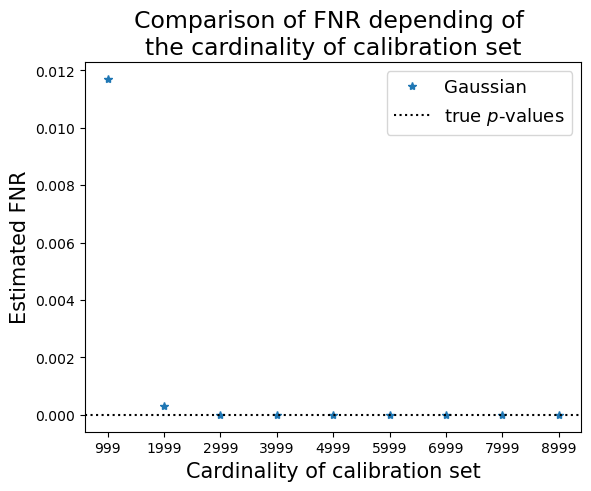
(d) $\Delta=3$, $m_{1}=5$

Figure 4: FNR as a function of the calibration set cardinality constrained to belong to $\mathcal{N}$.

For all the considered scenarios (Fig. 4(a), 4(b), 4(c), 4(d)), the FNR value converges to the value reached with true $p$-values (horizontal dashed line) as $n$ grows. From Figures 4(a) and 4(b), the convergence speed depends on the “difficulty” of the problem.

In practice, generating experiments similar to the ones illustrated by Figure 3.4.1 does not require to know the true reference distribution of the time series since is uses empirical $p$-values. However, the lack of labeled observations prevents us from computing the abnormality score and the actual FNR value, making the choice of the optimal value of $n$ highly challenging. To tackle this challenge our suggestion is to choose the largest possible value of $n$ that does not exceed the computation time limit. Doing that would output a value of $n$ minimizing the FNR criterion while meeting the computational constraints. However following this suggestion does not prevent us from computational drawbacks as illustrated by Figure 4(a) where the FNR optimal value is reached for $n=3999$ while choosing a larger $n$ does not bring any gain (but still increases the computational costs).

4 Global FDR control over the full time series

While working with streaming time series data, the anomaly detection problem requires to control the FDR value of the full time series to make sure that the global false alarm rate (FDR) remains under control at the end of the iterative process. The final criterion that is to be controlled is then the global FDR criterion given by

$$FDR_{1}^{\infty}(\hat{\varepsilon},\hat{p}),$$

where $\hat{\varepsilon}=(\hat{\varepsilon}_{t})_{t\geq 1}$ denotes a sequence of data-driven thresholds, and $\hat{p}$ stands for a sequence of empirical $p$-values (see Section 3 for further details). By contrast with this global objective, anomaly detection nevertheless requires making decision at each time step that is, for each new observation, without knowing what the next ones look like. This justifies the need for another (local) criterion that will be used to make a decision at each iteration, leading to the sequence of data-driven thresholds $\hat{\varepsilon}=(\hat{\varepsilon}_{t})_{t\geq 1}$. One additional difficulty results from the connection one needs to create between this local criterion and the (global) FDR of the full time series.

To this end, Section 4.1 starts by showing that controlling the FDR criterion for subseries of the full time series does not provide the desired global FDR control. Here “global” means “on the full time series” by contrast with the local FDR control, corresponding to controlling FDR for a strict subseries of the full one. Then Section 4.2 explores the connection between FDR for the full time series and the so-called modified-FDR (mFDR) for subseries. In particular, it turns out that controlling the mFDR value for all subseries of a given length $m$ yields the desired FDR control for the full time series. Section 4.3 then explains how the classical BH-procedure can be modified to get the mFDR control for subseries of length $m$, while Section 4.4 illustrates the practical behavior of the considered strategies on simulation experiments.

4.1 Local and global FDR controls are not equivalent

Let us consider a time series partitioned into 4 subseries as illustrated in Figure 5. The normal points are displayed in black and the anomalies in white. The surrounded points are those that have been detected as anomalies by the procedure.

Figure 5: Illustration of anomaly detection in subseries.

When computing the number of rejections, false positives and the False positive rate for each subseries, it comes

• Subseries 1 : 2 rejections, 1 false positive. $FDP_{1}^{4}=0.5$

• Subseries 2 : 2 rejections, 0 false positive. $FDP_{5}^{9}=0$

• Subseries 3 : 1 rejections, 1 false positive. $FDP_{10}^{14}=1$

• Subseries 4 : 1 rejections, 0 false positive. $FDP_{15}^{19}=0$

If one assumes that the same probability distribution has generated the observations within each subseries, the estimated (local) FDR can be defined as average of the successive FDP values for each subseries that is, $FDR_{1}^{4}=0.375$. Let us notice that the notation emphasizes that this FDR value is the average over subseries of respective length $m=4$. If one reproduces the same reasoning for the full time series, it comes: 6 rejections, two false positives, so that $FDP_{1}^{16}=1/3=0.333$. This example highlights that the FDP of the full time series is not equal to that of smaller subseries. This phenomenon gives some intuition on possible reasons why applying the classical BH-procedure on local windows of length $m$ (subseries) does control the FDR criterion for the individual subseries, but does not yield the desired global FDR control for the full time series. This intuition is confirmed by the boxplots of Figure 6, where $BH_{\alpha}$ has been applied on subseries of length $m=100$.

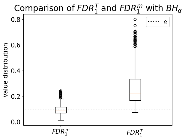
Figure 6: Comparison of the calculation of the FDR computed locally on a subseries and the FDR computed globally on the whole time series with Benjamini-Hochberg procedure applied on a subseries. This result is obtained by cutting a series of cardinality 1000 into 10 subseries of cardinality 100. Then the Benjamini-Hochberg procedure is applied on each subseries.

The left boxplot shows that $BH_{\alpha}$ provides the desired control at level $\alpha=10\%$ for each individual subseries of length $m$. However the right boxplot clearly departs from $\alpha$, meaning that the actual FDR value for the full times series of length $1\,000$ is strongly larger than $\alpha$ (more than 20% on average) leading to more false positives at the level of the full time series. The boxplots represent the quantile of FDP over 100 repetitions.

4.2 How mFDR can help in controlling the FDR of the full time series

4.2.1 Mixture model and time series

In this section one assumes that the time series is generated from a mixture process between a reference distribution $\mathcal{P}_{0}$ and an alternative distribution $\mathcal{P}_{1}$. The anomaly positions are supposed to be independent and generated by a Bernoulli distribution. This is a common assumption usually in the literature [28, 56] for simplification purposes.

Definition 4 (Time series process with anomalies).

Let $\pi\in[0,1]$ be the anomaly proportion and $\mathcal{P}_{0}$ and $\mathcal{P}_{1}$ be two probability distributions on the observation domain $\mathcal{X}$. $\mathcal{P}_{0}$ is the reference distribution and $\mathcal{P}_{1}$ denotes the alternative distribution. The generation process of a time series containing anomalies $(A_{t})_{t\geq 0}$ is given, for every $t\geq 0$, by

• $A_{t}\sim B(\pi)$ (Bernoulli distribution)

• if $A_{t}=0$, then $X_{t}\sim\mathcal{P}_{0}$.

• if $A_{t}=1$, then $X_{t}\sim\mathcal{P}_{1}$.

Moreover given the above scheme, $(X_{t})_{t\geq 0}$ is a random process with independent and identically distributed random variables $X_{t}\sim(1-\pi)\mathcal{P}_{0}+\pi\mathcal{P}_{1}$.

This definition details the way anomalies are generated. In particular it assumes that anomalies are independent from each other. Let us mention that this does not prevent us from observing a sequence of successive anomalies along the time series. However this scheme substantially differs from the case analyzed by [20] where specific patterns with successive anomalies are looked for.

4.2.2 Preliminary discussion: Disjoint and Overlapping subseries

In the context of online anomaly detection, the main focus in what follows is put on two situations where the data-driven thresholds $(\hat{\varepsilon}_{t})_{t\geq 0}$ can be defined from a set of $m$ empirical $p$-values: $(i)$ the disjoint case where disjoint subseries of length $m$ are successively considered, and $(ii)$ the overlapping case where the subseries (of length $m$) successively considered share $m-1$ common observations at each step.

Let us start with a subseries of length $m$ where each observation is summarized by its corresponding empirical $p$-value, and let us assume that there exists a function $f_{m}:$ $[0,1]^{m}\to[0,1]$ that is mapping a set of $m$ empirical $p$-values onto a real-valued random variable. This random variable corresponds to the data-driven threshold that is applied to the subseries of length $m$ to detect potential anomalies. This function $f_{m}$ is called the local threshold function since it outputs a threshold which applies to a subseries of length $m$.

Given the above notations, the threshold sequences $\hat{\varepsilon}_{d}=(\hat{\varepsilon}_{d,t})_{t}$ and $\hat{\varepsilon}_{o}=(\hat{\varepsilon}_{o,t})_{t}$ can be defined as follows.

• Disjoint subseries: $\hat{\varepsilon}_{d}:$ $t\mapsto\hat{\varepsilon}_{d,t}$ is given by

  $$\forall k\geq 0,\quad\forall t\in\llbracket km+1,(k+1)m\rrbracket,\quad\hat{\varepsilon}_{d,t}=f_{m}(\hat{p}_{km+1},\dots,\hat{p}_{(k+1)m})$$ (4.1)

• Overlapping subseries: $\hat{\varepsilon}_{o}:$ $t\mapsto\hat{\varepsilon}_{o,t}$ is given by

  $$\forall t\geq m,\qquad\hat{\varepsilon}_{o,t}=f_{m}(\hat{p}_{t-m+1},\dots,\hat{p}_{t}).$$ (4.2)

Figure 7 illustrates these two situations. In Figure 7(a), the full time series is split into small disjoint subseries of length $m$. $f_{m}$ is applied to each such subseries and the threshold is the same for all observations within a given subseries. Figure 7(b) displays the situation where overlapping subseries are successively considered. Because two successive subseries differ from each other by two observations, the thresholds are different at each time step unlike the disjoint case.

(a) Illustration of disjoint windows.

(b) Illustration of Overlapping sliding windows.

Figure 7: Comparison of disjoint window and overlapping window for the threshold function.

Furthermore the sequences $\hat{\varepsilon}_{d}$ and $\hat{\varepsilon}_{o}$ do not enjoy the same dependence properties. Figure 7(a) illustrates that all thresholds $\hat{\varepsilon}_{d,(k-1)m+1},\ldots,\hat{\varepsilon}_{d,km}$ are computed by applying $f_{m}$ to the same subseries $\hat{p}_{(k-1)m+1},\dots,\hat{p}_{km}$. Therefore only thresholds computed from different subseries are independent, while all thresholds from the same subseries are equal. In other words, $\hat{\varepsilon}_{d,t_{1}}$ and $\hat{\varepsilon}_{d,t_{2}}$ are independent if and only if $t_{1}$ and $t_{2}$ belong to different subseries that is, $\lfloor t_{1}/m\rfloor\neq\lfloor t_{2}/m\rfloor$, where $\lfloor\cdot\rfloor$ denotes the integer part. By contrast Figure 7(b) shows that the variables $\hat{\varepsilon}_{o,t}$ and $\hat{\varepsilon}_{o,t-1}$ are dependent because they share $m-1$ common observations. But all of them are still different and, for each $t$, $\hat{\varepsilon}_{o,t}$ is independent from $\hat{\varepsilon}_{o,t-m-1}$. This can be reformulated as $\hat{\varepsilon}_{o,t_{1}}$, $\hat{\varepsilon}_{o,t_{2}}$ are independent if and only if $|t_{1}-t_{2}|>m$.

In the present online anomaly detection context, considering the overlapping case sounds more convenient since the detection threshold can be updated at each time step (as soon as a new observation has been given), which makes the anomaly detector more versatile. However for technical reasons, next Section 4.2.3 still focuses disjoint subseries as a means to introduce important notions without introducing too many technicalities, while Section 4.2.4 extends the previous results to the more realistic case of overlapping subseries.

4.2.3 FDR control with disjoint subseries

As illustrated in Section 4.1, controlling FDR on each subseries of length $m$ (locally) is not equivalent to controlling FDR (globally) on the full time series. However in online anomaly detection, a decision has to be made at each time step regarding the potential anomalous status of each new observation. (This is a typical instance of a local decision since at step $t$, the decision making process ignores what will be observed at the next step.) This requires a criterion to be optimized locally (on subseries) in such a way that the resulting global FDR value (the one of the full time series) can be proved to be controlled at the desired level $\alpha$.

This requirement for a local criterion justifies the introduction of the modified FDR criterion, denoted by mFDR [63, 18], which is defined as follows.

Definition 5 (mFDR).

With the previous notations, the mFDR expression of the subseries from $t-m+1$ to $t$ is given by

$$mFDR_{t-m+1}^{t}(\hat{\varepsilon},\hat{p})=\frac{\mathbb{E}\left[\sum_{u\in\mathcal{H}_{0},t-m+1\leq u\leq t}\mathbb{1}[\hat{p}_{u}\leq\hat{\varepsilon}_{u}]\right]}{\mathbb{E}\left[\sum_{u=t-m+1}^{t}\mathbb{1}[\hat{p}_{u}\leq\hat{\varepsilon}_{u}]\right]},$$

where $\hat{\varepsilon}=(\hat{\varepsilon}_{u})_{t-m+1\leq u\leq t}$ denotes a sequence of thresholds, $\hat{p}$ is a sequence of empirical $p$-values evaluated at each observation of the subseries from $t-m+1$ to $t$.

Mathematically the difference between the mFDR and the FDR is that the expectation is no longer on the ratio but independently on the numerator and the denominator. The main interest for mFDR is clarified by Theorem 3, which establishes its connection to FDR. To be more specific, the control of the latter at the $\alpha$ level provides a global control of the FDR at the same level under simple conditions.

Theorem 3 (Global FDR control with disjoint subseries).

Assume that $\hat{\varepsilon}_{d}:$ $t\mapsto\hat{\varepsilon}_{d,t}$ is given by $\hat{\varepsilon}_{d,t}=f_{m}(\hat{p}_{km+1},\dots,\hat{p}_{(k+1)m})$, for any $t\in\llbracket km+1,(k+1)m\rrbracket$ ($k\geq 0$) and any integer $m\geq 1$ (see Eq. (4.1)). Let us also assume that the $p$-value random process $\hat{p}=(\hat{p}_{t})_{t\geq 1}$ follows the scheme detailed in Definition 4. Then, the global FDR value of the full (infinite) time series is equal to the local mFDR value of the any subseries of length $m$ from $t=km+1,k\in\mathbb{N}^{*}$. More precisely,

$$FDR_{1}^{\infty}(\hat{\varepsilon}_{d},\hat{p})=mFDR_{km+1}^{(k+1)m}(\hat{\varepsilon}_{d},\hat{p})=mFDR_{km+1}^{(k+1)m}(\hat{\varepsilon}_{d},\hat{p}).$$

Since the full time series is assumed to be infinite, Theorem 3 is an asymptotic result. It gives rise to a strategy for controlling the (asymptotic) FDR criterion at level $\alpha$ by means of successive local controls of mFDR on small subseries of length $m$. According to the asymptotic nature of Theorem 3, there is no particular constraint on the integer $m$. However when dealing within time series of a finite length $T$, the Theorem 3 proof suggests that choosing an $m$ “not too large” would be better since then, $k=T/m$ would take large values making the LLN applicable (see for instance Eq. (4.3)). Actually in the online anomaly detection context, practitioners only have a limited freedom regarding the choice of $m$. Therefore, for a given fixed $m$, the control of the FDR value of the full time series given by Theorem 3 will be all the more accurate as $T$ will be large. Fortunately this is not a limitation in the online anomaly detection context. The main limitation of Theorem 3 lies in the use of disjoint subseries, which sounds somewhat restrictive (at least from a practical perspective). This limitation will be overcome by next Theorem 4.

Proof of Theorem 3.

Let $k\geq 1$ denote an integer and $T=mk$. Then, the FDP definition and the $A_{t}$ variables introduced in Definition 4 justify that

$$FDP_{1}^{T}(\hat{\varepsilon}_{d},\hat{p})=\frac{FP_{1}^{T}(\hat{\varepsilon}_{d},\hat{p})}{R_{1}^{T}(\hat{\varepsilon}_{d},\hat{p})}=\frac{\sum_{t=1}^{T}\mathbb{1}[\hat{p}_{t}<\hat{\varepsilon}_{d,t}](1-A_{t})}{\sum_{t=1}^{T}\mathbb{1}[\hat{p}_{t}<\hat{\varepsilon}_{d,t}]},$$

where $R_{1}^{T}(\hat{\varepsilon}_{d},\hat{p})$ and $FP_{1}^{T}(\hat{\varepsilon}_{d},\hat{p})$ respectively denote the number of rejections (resp. false positives) at the threshold $\hat{\varepsilon}_{d}$ for the subseries $\hat{p}$.

Using the partitioning into $k$ subseries of length $m$, its first comes that $FP_{1}^{T}(\hat{\varepsilon}_{d},\hat{p})=\sum_{i=1}^{k}FP_{im-1}^{(i+1)m}(\hat{\varepsilon}_{d},\hat{p})$. It is also noticeable that the $k$ random variables $\{FP_{im-1}^{(i+1)m}(\hat{\varepsilon}_{d},\hat{p})\}_{1\leq i\leq k}$ are independent and identically distributed since the thresholds $\hat{\varepsilon}_{d,_{i}}$ remain unchanged within each subseries, they are identically distributed from one block to another, and the empirical $p$-values from different blocks are independent and identically distributed as well. Therefore the random variables $(FP_{im-1}^{(i+1)m}(\hat{\varepsilon}_{d},\hat{p}))_{1\leq i\leq k}$ are independent and identically distributed, which implies (Law of Large Numbers theorem) that, almost surely,

$$\lim_{k}\frac{1}{k}\sum_{i=1}^{k}FP_{im-1}^{(i+1)m}(\hat{\varepsilon}_{d},\hat{p})=\mathbb{E}[FP^{m}_{1}(\hat{\varepsilon}_{d},\hat{p})],$$ (4.3)

where the expectation is taken over all sources of randomness. (Here it is implicitly assumed that $T$ can go to $+\infty$.) Repeating the argument for$R_{1}^{T}(\hat{\varepsilon}_{d},\hat{p})$, it also comes that

$$\mathbb{E}[R^{m}_{1}(\hat{\varepsilon}_{d},\hat{p})]=\lim_{k}\frac{1}{k}\sum_{i=1}^{k}R_{im-1}^{(i+1)m}(\hat{\varepsilon}_{d},\hat{p}),\qquad a.s..$$

The conclusion then results from noticing that

$$mFDR_{1}^{m}(\hat{\varepsilon}_{d},\hat{p}) =\frac{E[FP_{1}^{m}(\hat{\varepsilon}_{d},\hat{p})]}{E[R_{1}^{m}(\hat{\varepsilon}_{d},\hat{p})]}=\lim_{k}\frac{\sum_{i=1}^{k}FP_{im-1}^{(i+1)m}(\hat{\varepsilon}_{d},\hat{p})}{\sum_{i=1}^{k}R_{im-1}^{(i+1)m}(\hat{\varepsilon}_{d},\hat{p})}=\lim_{T}FDP_{1}^{T}(\hat{\varepsilon}_{d},\hat{p}).$$

∎

4.2.4 FDR control with overlapping windows

Unlike previous Theorem 3, following Theorem 4 establishes a similar control of the global FDR criterion on the full time series by means of successive local controls of the mFDR criterion on subseries that are allowed to overlap each other. This is closer to the practical situation arising in online anomaly detection where one new observations is collected at each time step, inducing a shift by one of the set of observations for which a decision has to be made.

Theorem 4 (Global FDR control with overlapping subseries).

Assume that $\hat{\varepsilon}_{o}:$ $t\mapsto\varepsilon_{o,t}$ is given by $\hat{\varepsilon}_{o,t}=f_{m}(\hat{p}_{t-m+1},\dots,\hat{p}_{t})$, for any $t\geq 1$, with $f_{m}:$ $[0,1]^{m}\to[0,1]$ permutation invariant (see Eq. (4.1)). Let us also assume that the $p$-value random process $\hat{p}=(\hat{p}_{t})_{t\geq 1}$ follows the scheme detailed in Definition 4 and there exists $n$ such that $|t_{1}-t_{2}|>n$ implies that $\hat{p}_{t_{1}}$ and $\hat{p}_{t_{2}}$ are independent. Then, the global FDR value of the full (infinite) time series is equal to the local mFDR value of the any subseries of length $m$ computed at time $t\in\mathbb{N}^{*}$. More precisely

$$FDR_{1}^{\infty}(\hat{\varepsilon}_{o},\hat{p})=mFDR_{t-m+1}^{t}(\hat{\varepsilon}_{o},\hat{p})=mFDR_{1}^{m}(\hat{\varepsilon}_{o},\hat{p})$$

Theorem 4 gives a similar result to the one of Theorem 3 but in a more realistic framework corresponding to the real time anomaly detection context. In particular the main improvement lies in that a threshold can be recomputed at each time step from a (shifted) subseries of length $m$. An important consequence is that the desired control for the FDR of the full (infinite) time series at level $\alpha$ can be achieved provided one can control the successive mFDR of all (shifted) subseries of length $m$ at level $\alpha$. This point is not obvious at all and constitutes the main concern of Section 4.3 where a new multiple testing procedure is designed to yield the desired control of the mFDR criterion. The main limitation of Theorem 4 is the requirement that $f_{m}$ has to be permutation invariant. Let us emphasize that this property holds true with the BH-procedure for instance. Let us also mention that the empirical $p$-values for instance computed as $\hat{p}_{t}=\hat{p}\mbox{-value}(X_{t},\{X_{t-n},\ldots,X_{t-1}\})$ actually satisfy the requirements of Theorem 4 regarding the independence and the stationarity.

Proof of Theorem 4.

Let us start with the FDP expression for a time series of length $T$.

$$FDP_{t=1}^{T} =\frac{\sum_{t=1}^{T}\mathbb{1}[\hat{p}_{t}<\hat{\varepsilon}_{o,t}](1-A_{t})}{\sum_{t=1}^{T}\mathbb{1}[\hat{p}_{t}<\hat{\varepsilon}_{o,t}]}$$

$$=\frac{\frac{1}{T}\sum_{t=1}^{T}\mathbb{1}[\hat{p}_{t}<f_{m}(\hat{p}_{t-m+1}^{t})](1-A_{t})}{\frac{1}{T}\sum_{t=1}^{T}\mathbb{1}[\hat{p}_{t}<f_{m}(\hat{p}_{t-m+1}^{t})]},$$

where $f_{m}(\hat{p}_{i}^{j})=f_{m}(\hat{p}_{i},\ldots,\hat{p}_{j})$, for $i<j$. Since the decision process $(\mathbb{1}[\hat{p}_{t}<\hat{\varepsilon}_{o,t}])_{t}$ and the false positives process $(\mathbb{1}[\hat{p}_{t}<\hat{\varepsilon}_{o,t}]A_{t})_{t}$ are not independent.

Therefore it is not possible to use the Law of Large Numbers as in the proof of Theorem 3. The alternative strategy consists first in splitting the numerator and denominator into several disjoint subseries corresponding to independent and identically distributed processes. Then partitioning the times series of length $T=T^{\prime}(n+m)$ into $T^{\prime}$ subseries, each of length $n+m$, it results that

$$\frac{1}{T}\sum_{t=1}^{T}\mathbb{1}[\hat{p}_{t}<f_{m}(\hat{p}_{t-m+1}^{t})](1-A_{t})$$

$$=\frac{1}{n+m}\sum_{k=1}^{n+m}\left(\frac{1}{T^{\prime}}\sum_{t=0}^{T^{\prime}-1}\mathbb{1}[\hat{p}_{t(n+m)+k}<f_{m}(\hat{p}_{t(n+m)+k-m+1}^{t(n+m)+k})](1-A_{t(n+m)+k})\right).$$ (4.4)

Interestingly for each $k$ from 1 to $m+n$, the summands within the brackets do all belong to different subseries, which makes the sum over $t$ a sum of independent and identically distributed random variables. It results that, for each $1\leq k\leq n+m$, the average within the brackets is converging to its expectation by the LLN theorem.

Since the limit of a (finite) sum is equal to the sum of the limits, the average in Eq. (4.4) is converging and

$$\lim_{T\rightarrow\infty}\frac{1}{T}\sum_{t=1}^{T}\mathbb{1}[\hat{p}_{t}<\hat{\varepsilon}_{o,t}](1-A_{t}) =\sum_{k=1}^{m}\mathbb{E}\left[\mathbb{1}[\hat{p}_{k}<\hat{\varepsilon}_{o,k}](1-A_{k})\right]\mbox{ a.s.}$$

$$=m\mathbb{E}\left[\mathbb{1}[\hat{p}_{m}<\hat{\varepsilon}_{o,m}](1-A_{m})\right]\mbox{ a.s.}.$$

Then after applying the same reasoning on the denominator, it gives:

$$FDP_{1}^{\infty}(\hat{\varepsilon}_{o},\hat{p})=\frac{\mathbb{E}\left[\mathbb{1}[\hat{p}_{m}<\hat{\varepsilon}_{o,m}](1-A_{m})\right]}{\mathbb{E}\left[\mathbb{1}[\hat{p}_{m}<\hat{\varepsilon}_{o,m}]\right]}$$

What remains to show is to proof that:

$$\frac{\mathbb{E}\left[\mathbb{1}[\hat{p}_{m}<\hat{\varepsilon}_{o,m}](1-A_{m})\right]}{\mathbb{E}\left[\mathbb{1}[\hat{p}_{m}<\hat{\varepsilon}_{o,m}]\right]}=mFDR_{1}^{m}(\hat{\varepsilon}_{o},\hat{p})$$

This result comes from the stationarity of $\hat{p}$ and the permutation invariance of $f_{m}$. These properties imply that all $p$-values inside a subseries have the same probability to be rejected.

$$\forall t\in\llbracket 1,m\rrbracket,\quad\mathbb{E}[\mathbb{1}[\hat{p}_{t}<f_{m}(\hat{p}_{1}^{m})](1-A_{t})]=\mathbb{E}[\mathbb{1}[\hat{p}_{m}<f_{m}(\hat{p}_{1}^{m})](1-A_{m})]$$ (4.5)

Which imply

$$\mathbb{E}[\sum_{t=1}^{m}\mathbb{1}[\hat{p}_{t}<f_{m}(\hat{p}_{1}^{m})](1-A_{t})]=m\mathbb{E}[\mathbb{1}[\hat{p}_{m}<f_{m}(\hat{p}_{1}^{m})](1-A_{m})]$$ (4.6)

Using the same argument for the denominator, is gives:

$$\frac{\mathbb{E}\left[\mathbb{1}[\hat{p}_{m}<\hat{\varepsilon}_{o,m}](1-A_{m})\right]}{\mathbb{E}\left[\mathbb{1}[\hat{p}_{m}<\hat{\varepsilon}_{o,m}]\right]} =\frac{m\mathbb{E}\left[\mathbb{1}[\hat{p}_{m}<\hat{\varepsilon}_{o,m}](1-A_{m})\right]}{m\mathbb{E}\left[\mathbb{1}[\hat{p}_{m}<\hat{\varepsilon}_{o,m}]\right]}$$ (4.7)

$$=\frac{\mathbb{E}[\sum_{t=1}^{m}\mathbb{1}[\hat{p}_{t}<f_{m}(\hat{p}_{1}^{m})](1-A_{t})]}{\mathbb{E}[\sum_{t=1}^{m}\mathbb{1}[\hat{p}_{t}<f_{m}(\hat{p}_{1}^{m})]]}$$ (4.8)

$$=mFDR_{1}^{m}(\hat{\varepsilon}_{o},\hat{p})$$ (4.9)

∎

4.3 Modified BH-procedure and mFDR control

As shown in Section 4.2, controlling the FDR value of the full time series is possible. The strategy then consists in first controlling the mFDR criterion of all successive subseries of length $m$ along the full time series at level $\alpha$. The main challenge addressed in the present section is to design a new multiple testing procedure that controls the local mFDR criterion at a prescribed level $\alpha$.

In Section 4.3.1, it is proved that applying the classical BH-procedure on a time series of length $m$ does not yield the control of mFDR at level $\alpha$. However the proof of this result gives rise to a strategy for modifying the classical BH-procedure (Section 4.3.3) in a such a way that applying the so-called modified BH-procedure provides the desired mFDR control at level $\alpha$.

4.3.1 mFDR control with the BH-procedure

Next Proposition 3 establishes the actual mFDR level achieved by the BH-procedure.

Proposition 3.

Let $(X_{i})_{1}^{m}$ satisfy the requirements detailed by Definition 4. Let $(p_{1},\ldots,p_{m})$ be the true $p$-values corresponding to a subseries of length $m$ that is, for any $1\leq i\leq m$, $p_{i}=\mathbb{P}_{X\sim\mathcal{P}_{0}}(X\geq X_{i})\in[0,1]$. Then for every $\alpha\in[0,1]$, applying $BH_{\alpha}$ on the $p$-values $(p_{i})_{1\leq i\leq m}$ leads to

$$mFDR_{1}^{m}(p)=\frac{\alpha m_{0}}{m}\frac{\mathbb{E}R_{1,\alpha}^{m}(1)}{\mathbb{E}R_{1,\alpha}^{m}},$$

where $R_{1,\alpha}^{m}(1)=\left|BH_{\alpha}(0,p_{2},..,p_{m})\right|$ and $R_{1,\alpha}^{m}=\left|BH_{\alpha}(p_{1},p_{2},..,p_{m})\right|$, with $|S|$ denoting the cardinality of the set $S$.

If the ratio $\mathbb{E}R(1)^{m}(1)/\mathbb{E}R(1)^{m}$ were known, it could be possible to control of the $mFDR$ criterion at level $\alpha$ by simply applying the BH-procedure with a preliminary level $\alpha^{\prime}=\frac{m}{m_{0}}\frac{\mathbb{E}R_{1,\alpha}}{\mathbb{E}R_{\alpha}}\alpha$. Unfortunately at this stage, this ratio is not known and the latter strategy cannot be straightforwardly applied. Deriving such a modified BH-procedure is the purpose of the next sections. Let us also recall that in the anomaly detection context, $m_{0}$ is unknown but expected to be close to $m$ since only a few anomalies are usually expected. Therefore the main challenge remains to compute $\mathbb{E}R(1)^{m}(1)/\mathbb{E}R(1)^{m}$.

Proof of Proposition 3.

The mFDR formula is given by

$$mFDR_{1}^{m}(p)=\frac{\mathbb{E}[FP_{1,\alpha}^{m}(p)]}{\mathbb{E}[R_{1,\alpha}^{m}(p)]}.$$

Let us compute the numerator $\mathbb{E}[FP_{1}^{m}(p)]$ value after applying the $BH_{\alpha}$. For simplification purposes, let $R=R_{1,\alpha}^{m}(p)$ (respectively $FP_{1}^{m}(p)=FP_{1,\alpha}^{m}(p)$) denote the number of rejections (resp. of false positives) resulting from $BH_{\alpha}$. Introducing $D_{i}=\mathbb{1}[p_{i}\leq\frac{R}{m}\alpha]$, it appears that

$$FP_{1}^{m}(p) =\sum_{i=1}^{m}(1-A_{i})D_{i}.$$

Now focusing on $D_{i}$ and using $R(i)$, the (random) number of rejections output by $BH_{\alpha}$ when the $p_{i}$ is replaced by 0, it comes that

$$D_{i}=\sum_{k=1}^{m}\mathbb{1}[p_{i}\leq\frac{k}{m}\alpha]\mathbb{1}[R=k] =\sum_{k=1}^{m}\mathbb{1}[p_{i}\leq\frac{k}{m}\alpha]\mathbb{1}[R(i)=k],$$

since, on the event $\{R=k\}$, $p_{i}$ is already rejected that is, $p_{i}\leq\frac{k}{m}\alpha$. Taking the conditional expectation given $p$ except $p_{i}$ on both sides, it results

$$\mathbb{E}[D_{i}|p\backslash p_{i}]=\sum_{k=1}^{m}\mathbb{P}[p_{i}\leq\frac{k}{m}\alpha]\mathbb{1}[R(i)=k] =\frac{\alpha}{m}\sum_{k=1}^{m}k\mathbb{1}[R(i)=k]$$

since the true $p$-value $p_{i}$ follows a uniform distribution on $[0,1]$. Now integrating over all remaining $p$-values yields that

$$\mathbb{E}[D_{i}]=\frac{\alpha}{m}\sum_{k=1}^{m}k\mathbb{P}[R(i)=k] =\frac{\alpha}{m}\mathbb{E}[R(i)].$$

Since $A_{i}$ and $D_{i}$ are independent random variables, it results that

$$\mathbb{E}[FP_{1}^{m}(p)] =\sum_{i=1}^{m}\mathbb{E}[(1-A_{i})\mathbb{E}[D_{i}\mid A_{i}]]=\sum_{i=1}^{m}\mathbb{E}[(1-A_{i})\mathbb{E}[D_{i}]]$$

$$=\frac{\alpha}{m}\mathbb{E}[R(1)]\sum_{i=1}^{m}\mathbb{E}[1-A_{i}]$$

$$=\alpha\frac{m_{0}}{m}\mathbb{E}[R(1)],$$

where the last-but-one equality stems from the fact that all random variables $R(i)$ are identically distributed. ∎

4.3.2 Evaluating the ratio of rejection numbers

Previous Section 4.3.1 raises the importance of the ratio $\mathbb{E}R_{1,\alpha}^{m}(1)/\mathbb{E}R_{1,\alpha}^{m}$ of rejection numbers. The present section aims at deriving a numeric approximation to this ratio. In a first step, a first result details the value of the denominator. In a second step, an approximation to the numerator is derived based on a heuristic argument and also empirically justified on simulation experiments.

Calculating the expected number of rejections

When $mFDR$ is assumed to equal $\alpha$, the expected number of rejections can be made explicit.

Proposition 4.

With the previous notation, let $(X_{1},\ldots,X_{m})$ be given by Definition 4, where $\pi$ denotes the unknown proportion of anomalies, and assume that $mFDR_{1}^{m}=\alpha$ and $FNR_{1}^{m}=\beta\in[0,1]$. Then

$$\mathbb{E}[R_{1,\alpha}^{m}]=\frac{m\pi(1-\beta)}{1-\alpha}.$$ (4.10)

The proof is postponed to Appendix A.5. For instance, Eq. (4.10) establishes that the expected number of rejection output by $BH_{\alpha}$ increases with $\pi$, the unknown proportion of anomalies along the signal. This makes sens since the more anomalies, the more expected rejections. The expected number of rejection is also increasing with $\alpha$: the larger $\alpha$, the less restrictive the threshold, and the more rejections should be made. However the number of rejection decreases with the FNR value $\beta$. As $\beta$ increases, the proportion of false negatives grows meaning that fewer alarms are raised, which results in a smaller number of rejections.

Heuristic arguments

In what follows, the assumption is made that anomalies are easy to detect, meaning that the $FNR_{1}^{m}$ value $\beta$ is negligible compared to 1. In this context, Proposition 4 would yield that

$$\mathbb{E}[R_{1,\alpha}^{m}]\approx\frac{m\pi}{1-\alpha}.$$ (Power)

An another assumption is also made about the relationship between $\mathbb{E}[R_{1,\alpha}^{m}]$ and $\mathbb{E}[R_{1,\alpha}^{m}(i)]$. This assumption is based on a heuristic argument supported by the results of numerical experiments as reported in Table 3. In what follows, it is assumed that

$$\mathbb{E}[R_{1,\alpha}^{m}(i)]=\mathbb{E}[R_{1,\alpha}^{m}]+1.$$ (Heuristic)

No mathematical proof of this statement is given in the present paper. However, Table 3 displays numerical values which empirically support this approximation, whereas further analyzing the connection between these quantities should be necessary.

$BH_{\alpha}$	$0.05$	$0.1$	$0.2$
$\mathbb{E}[R_{1,\alpha}^{m}]$	2.14	2.32	2.78
$\mathbb{E}[R_{1,\alpha}^{m}(i)]$	3.18	3.44	3.99

Table 3: Numerical evaluations for different values of $\alpha$ ($10^{3}$ repetitions)

Let us emphasize that Table 3 has been obtained with Gaussian data (generated similarly to those detailed in Section 3.4). For all the three considered values of $\alpha$, one observes that $\mathbb{E}[R(1)]$ remains close to (but also slightly larger than) $\mathbb{E}[R]+1$.

From now on and in all what follows, (Heuristic) is assumed to hold true. In particular, (Heuristic) gives rise to a strategy for computing the ratio $\frac{\mathbb{E}[R(1)]}{\mathbb{E}[R]}$. So all ingredient to build a procedure that control the mFDR are given.

4.3.3 Modified BH

From previous Sections 4.3.1 and 4.3.2, it is now possible to suggest and analyze the new modified BH-procedure (mBH in the sequel).

Definition 6 (Modified BH-procedure (mBH)).

Let $m$ be an integer and $\alpha\in[0,1]$. Let us introduce the level $\alpha^{\prime}=\alpha(1+\frac{1-\alpha}{m\pi})^{-1}$, where $\pi\in[0,1]$ denotes the unknown proportion of anomalies (see Definition 4. Let us further assume (Power) and (Heuristic) hold true. Then the modified BH-procedure, denoted by $mBH_{\alpha}$, is given for all true $p$-values $(p_{1},\ldots,p_{m})\in[0,1]^{m}$ by,

$$mBH_{\alpha}(p_{1},\ldots,p_{m})=BH_{\alpha^{\prime}}(p_{1},\ldots,p_{m}).$$

The related $mBH_{\alpha}$ threshold at level $\alpha$ is defined as

$$\varepsilon_{mBH_{\alpha}}=\varepsilon_{BH_{\alpha^{\prime}}},$$

when computed with true $p$-values, and $\hat{\varepsilon}_{mBH_{\alpha}}=\hat{\varepsilon}_{BH_{\alpha^{\prime}}}$ when used with empirical $p$-values.

The above definition defines the $mBH_{\alpha}$ in terms of the BH-procedure by simply changing the level of control $\alpha^{\prime}$. This new level value depends on the unknown proposition $\pi$ of anomalies. Since in realistic anomaly detection scenarios observations are not labeled, [57] provides guidelines on how $\pi$ could be estimated. From Proposition 4, it also appears that $\alpha^{\prime}=\alpha(1+\frac{1-\alpha}{m\pi(1-\beta)})^{-1}$ should arise as the ideal threshold. However since $\beta$ is unknown, (Power) leads to the approximation suggested within the above definition.

Corollary 5 (Control of the FDR using mBH).

Under the same notations and assumptions as Theorem 4. Let $m$ and $\ell$ be two integers and assuming (Power) and (Heuristic) hold, let $n$ and $\alpha^{\prime}$ be defined by

$$\alpha^{\prime}=\frac{\alpha}{1+\frac{1-\alpha}{m\pi}}\quad\mbox{ and }\quad n=\ell m/\alpha^{\prime}-1.$$

the next two results hold true.

1. If the FDR can be controlled at level $\alpha^{\prime}$ on subseries of size $m$, using $BH_{\alpha^{\prime}}$: $FDR_{1}^{m}(\hat{\varepsilon}_{BH_{\alpha^{\prime}}},\hat{p})=(1-\pi)\alpha^{\prime},$ then the FDR of the whole time series can be controlled at the level $\alpha$ using $mBH_{\alpha}$

   $$FDR_{1}^{\infty}(\hat{\varepsilon}_{mBH_{\alpha}},\hat{p})=(1-\pi)\alpha$$ (4.11)

2. If $FDR_{1}^{m}(\hat{\varepsilon}_{BH_{\alpha^{\prime}}},\hat{p})\leq(1-\pi)\alpha^{\prime}$ . Then, the FDR of the whole time series can be controlled at the level $\alpha$

   $$FDR_{1}^{\infty}(\hat{\varepsilon}_{mBH_{\alpha}},\hat{p})\leq(1-\pi)\alpha$$ (4.12)

Proof of Corallary 5.

All conditions being satisfied Theorem 4 gives that:

$$FDR_{1}^{\infty}(\hat{\varepsilon}_{mBH_{\alpha}},\hat{p})=mFDR_{1}^{m}(\hat{\varepsilon}_{mBH_{\alpha}},\hat{p})$$ (4.13)

By definition of $mBH_{\alpha}$ in Definition 6 and with Proposition 3:

$$mFDR_{1}^{m}(\hat{\varepsilon}_{mBH_{\alpha}},\hat{p}) =mFDR_{1}^{m}(\hat{\varepsilon}_{BH_{\alpha^{\prime}}},\hat{p})$$

$$=\frac{\mathbb{E}[R(1)]}{\mathbb{E[R]}}FDR_{1}^{m}(\hat{\varepsilon}_{BH_{\alpha^{\prime}}},\hat{p})$$

Under the assumptions Heuristic and Power, it gives:

$$\frac{\mathbb{E}[R(1)]}{\mathbb{E}[R]} =1+\frac{1-\alpha}{m\pi}$$

$$mFDR_{1}^{m}(\hat{\varepsilon}_{mBH_{\alpha}},\hat{p}) =(1+\frac{1-\alpha}{m\pi})FDR_{1}^{m}(\hat{\varepsilon}_{BH_{\alpha^{\prime}}},\hat{p})$$

From hypothesis $FDR_{1}^{m}(\hat{\varepsilon}_{BH_{\alpha^{\prime}}},\hat{p})=(1-\pi)\alpha^{\prime}$. Replacing the value of $\alpha^{\prime}$ with its expression it gives:

$$mFDR_{1}^{m}(\varepsilon_{mBH_{\alpha}})=(1+\frac{1-\alpha}{m\pi})(1-\pi)(1+\frac{1-\alpha}{m\pi})^{-1}\alpha=(1-\pi)\alpha$$

Plugin this result into Eq. 4.13 this gives desired result.

$$FDR_{1}^{\infty}(\hat{\varepsilon}_{mBH_{\alpha}},\hat{p})=(1-\pi)\alpha$$

∎

The next result shows how $mBH_{\alpha}$ can be applied to reach a global FDR control for the full time series at the desired level. It applies Corollary 5 by specifying different ways to estimate $p$-values on the time series.

Theorem 5 (Global FDR control using $mBH_{\alpha}$).

Let $(X_{t})$ be a mixture process introduced in Definition 4, with $\pi$ denoting the anomaly proportion. Let $\alpha\in[0,1]$ be the desired FDR level for the full time series. For $m$ and $\ell$ two integers and assuming (Power) and (Heuristic) hold, let $n$ and $\alpha^{\prime}$ be defined by

$$\alpha^{\prime}=\frac{\alpha}{1+\frac{1-\alpha}{m\pi}}\quad\mbox{ and }\quad n=\ell m/\alpha^{\prime}-1.$$

If $(\hat{p}_{t})$ are given following one of the schemes

1. $\hat{p}_{t}=1-\mathbb{P}_{X\sim\mathcal{P}_{0}}(a(X)>a(X_{t}))$

2. $\hat{p}_{t}=\hat{p}\mbox{-value}(X_{t},\{Z_{t,1},\ldots,Z_{t,n}\})$ with $Z_{t,i}\sim\mathcal{P}_{0}$

then,

$$FDR_{1}^{\infty}(\hat{\varepsilon}_{mBH_{\alpha}},\hat{p})=(1-\pi)\alpha.$$

Otherwise, if $(\hat{p}_{t})$ are given by

1. $\hat{p}_{t}=\hat{p}\mbox{-value}(X_{t},\{(1-A_{t-n+1})X_{t-n+1}+A_{t-n+1}Z_{t,1},\ldots,(1-A_{t})X_{t}+A_{t}Z_{t,n}\})$ with $Z_{t,i}\sim\mathcal{P}_{0}$ ,

then,

$$FDR_{1}^{\infty}(\hat{\varepsilon}_{mBH_{\alpha}},\hat{p})\leq(1-\pi)\alpha.$$

The main merit of Theorem 5 is to establish the actual level of control for the global FDR of the full time series depending on the type of empirical $p$-value used in the anomaly detection process. This level of control depends on the unknown proportion $\pi$ of anomalies. Therefore if $\pi$ is close to 0 (only a few anomalies are expected), then the FDR control is close to $\alpha$. However, since alpha’ is close to 0 when pi is close to 0, an estimation of $\pi$ (or expert knowledge) is required to detect anomalies. Some guidelines are provided in [57]. The last type of empirical $p$-values is (almost) the one which is used in practice in the present work. More precisely Section 5.2.3 describes empirical $p$-values based on a “Sliding Calibration Set”.

Proof of Theorem 5.

The Corollary 5 gives the two properties that the $p$-values families has to verify to control the FDR of the time series:

• The $p$-values are stationary and independent when time distance is larger than $n$.

• The FDR is controlled at level $\alpha^{\prime}$ on subseries of size $m$: $FDR(\hat{\varepsilon}BH_{1}^{\alpha^{\prime}},\hat{p})=(1-\pi)\alpha^{\prime}$

In the following, these properties are verified for the different $p$-values.

1. The true $p$-value family is i.i.d., because the time series mixture is i.i.d. Also the Theorem 1 gives the control for subseries. Using Corollary 5 the FDR of the whole time series is controlled at level $(1-\pi)\alpha$.

2. This $p$-value family is i.i.d., because the time series mixture is i.i.d. and the calibration sets are also i.i.d. Using the Theorem 1, it gives the FDR control on subseries. With Corollary 5 the FDR of the whole time series is controlled at level $(1-\pi)\alpha$.

3. This $p$-value family is not i.i.d. However, because the calibration are build using a sliding window of size $n$, two $p$-values $p_{t_{1}}$ and $p_{t_{2}}$ are independent when $|t_{1}-t_{2}|>m$. The calibration sets of the $p$-values overlapped, Then Corollary 4 ensures the upper bound of the FDR for subseries of size $m$. With Corollary 5 the FDR of the whole time series is upper bounded controlled at level $(1-\pi)\alpha$.

∎

4.4 Empirical results

In this section, the abilities to get local control of the mFDR and the global control of the FDR, using mBH are assessed empirically. Corollary 5 and Theorem 5 give theoretical results about the control of the mFDR for subseries under the assumptions Power and Heuristic. However, these assumptions are hard to ensure in practice. In Section 4.4.1, the assessment is done on simulated data where the level of atypicity of the anomalies varies from one sample to another. Different scenarios are tested to verify if the mFDR control hold. Theorem 3 and Theorem 4 give FDR control over the full time series. In Section 4.4.2, the abilities of thresholds computed on disjoint and overlapping subseries to control the mFDR using are compared. Theorem 3 and Theorem 4 give asymptotic FDR control over the full time series. But there is no result about the speed of convergence, which is necessary when used on finite time series. In Section 4.4.3, the FDR for the full time series is calculated across different situations, as a function of time series size. It is possible to figure out when the entire series reaches control of the FDR.

4.4.1 Control of the mFDR on disjoint subseries

Experiment description

From Corollary 5 the $mBH_{\alpha}$ controls the $mFDR_{1}^{m}$ only if the Power assumption is satisfied. Since the power of the anomaly detector depends on how easy it is to detect anomalies, the level of atypicity $\delta$ is introduced. To quantifies the atypicity of a data point $X_{t}$, the true $p$-value is computed as $p_{t}=\mathbb{P}_{X\sim\mathcal{P}_{0}}(X>X_{t})$, and the atypicity level is defined as the inverse of the $p$-value: $\delta_{t}=1/p_{t}$. The atypicity level is preferred over the $p$-values because it is easier to show on the x-axis of the chart, when the $p$-value is small. To evaluate the effect of power, for each sample all anomalies have their level of atypicity lower bounded a given parameter $\delta$. Therefore, it is possible to observe the effect of a variation in the level of atypicity on the $mFDR_{1}^{m}$, $FDR_{1}^{m}$ and $FNR_{1}^{m}$.

For a given scenario—meaning a proportion of anomalies $\pi$, a level of atypicity $\delta$, and a desired level of mFDR noted $\alpha$—the actual mFDR, FDR, and FNR are estimated. These quantities are estimated using $K=50$ samples of $m$ data points. To control the estimation error made when estimating on a finite number of samples, each estimation is repeated $B=100$ times. The estimation proceeds as follows:

1. With $1\leq b\leq B$, and $1\leq k\leq K$, $m$ data point are generated.

   • $m_{0}$ normal data $p_{b,k,1},\ldots,p_{b,k,m_{0}}$ are generated according the reference law $U([0,1])$.

   • $m_{1}$ abnormal data $p_{b,k,m_{0}+1},\ldots,p_{b,k,m}$ are generated using the alternative law $U([0,1/\delta])$, with $\delta$ the level of atypicity of the anomalies.

2. Then, for each sample, the thresholds are estimated with BH and mBH procedures:

   • $\hat{\varepsilon}_{b,k,BH}=BH_{\alpha}(p_{b,k,1},\ldots,p_{b,k,m})$,

   • $\hat{\varepsilon}_{b,k,mBH}=mBH_{\alpha}(p_{b,k,1},\ldots,p_{b,k,m})$.

3. The number of rejections, false positives and false negatives are computed on each sample and according each threshold. Using $M\in\{mBH,BH\}$:

   • $R_{b,k,M}=\sum_{i=1}^{m}\mathbb{1}[p_{b,k,i}\leq\hat{\varepsilon}_{b,k,M}]$,

   • $FP_{b,k,M}=\sum_{i=1}^{m_{0}}\mathbb{1}[p_{b,k,i}\leq\hat{\varepsilon}_{b,k,M}]$,

   • $FN_{b,k,M}=\sum_{i=m_{0}+1}^{m}\mathbb{1}[p_{b,k,i}>\hat{\varepsilon}_{b,k,M}]$.

4. The FDR, mFDR and FNR are estimated by averaging results over the $K$ samples:

   • $FDR_{b,M}=\frac{1}{K}\sum_{k=1}^{K}\frac{FP_{b,k,m}}{R_{b,k,m}}$,

   • $mFDR_{b,M}=\frac{\sum_{k=1}^{K}FP_{b,k,m}}{\sum_{k=1}^{K}R_{b,k,m}}$,

   • $FNR_{b,M}=\frac{1}{K}\sum_{k=1}^{K}\frac{FN_{b,k,m}}{m_{1}}$.

These steps are then repeated over the different scenarios.

Results and Analysis

The results are shown in Figure 8 by varying $\delta$, $\alpha$ and $m_{1}$. In Figure 8, the level of atypicity $\delta$ in represented in the abscissa. The ordinate represents the estimated mFDR (in Figure 8(a) or 8(c)) or FNR (in Figure 8(b) or 8(d)). Different colors are used to distinguish between BH and mBH procedures.

For a low level of atypicity $\delta$, the FNR and the mFDR are high because the anomalies are difficult to detect. By increasing $\delta$, the FNR and the mFDR decrease. As shown in Figure 8(b), with values of $\delta$ around $100$, the FNR is equal to $0$ which can also generate a constant mFDR as shown in Figure 8(a). For the mBH-procedure, the mFDR is constant and equal to $\alpha$. This is consistent with Theorem 4, which guarantees the control at level $\alpha$ when all anomalies are detected.

Figure 8(d) shows the totality of the anomalies detected for $\delta=2000$. The same result in figure 8(b) with $\delta=100$. This is explained by the different parameters of the experiment. The easier the anomalies are detected, faster the $FNR=0$ is reached for a small $\delta$ and therefore the easier it is to guarantee $mFDR=\alpha$.

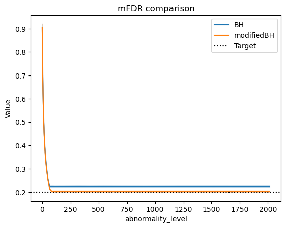
(a) mFDR, $\alpha=0.2$, $\pi=0.07$

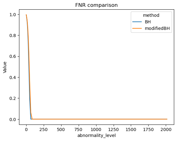
(b) FNR, $\alpha=0.2$, $\pi=0.07$

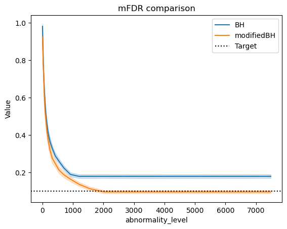
(c) mFDR, $\alpha=0.1$, $\pi=0.01$

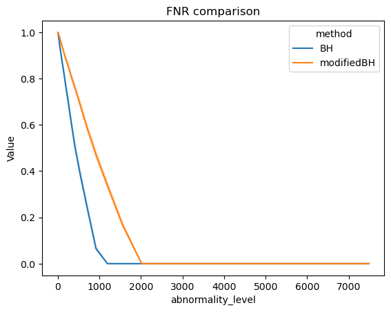
(d) FNR, $\alpha=0.1$, $\pi=0.01$

Figure 8: mFDR and FNR as a function of level of atypicity across different scenarios

Conclusion

In order to control the mFDR at the desired level $\alpha$ using mBH, the FNR has to be equal to 0. The capacity of mBH to control the mFDR depends of the difficulty of the problem. When abnormality proportion and level of atypicity are lower, the power of mBH decreases and the mFDR is harder to control. The results of this experiment gives an idea of the atypicity level that the detector can find.

4.4.2 Disjoint subseries vs overlapping subseries

Experiment Description

Theorems 3 and 4 theoretically prove the control of the FDR over the full time series throw control of the mFDR over disjoint subseries or overlapping subseries. According Corollary 5, the procedure $mBH_{\alpha}$ allows the control of the mFDR over subseries under assumption Heuristic and Power that are hard to verify. Empirical results from Section 4.4.1 show that control of mFDR for the disjoint subseries can be obtained for scenarios where the level of atypicity $\delta$ is high enough. It still unknown whether these results hold true in cases where the subseries overlap In this section FDR control throw disjoint and overlapping subseries are compared.

For each scenario, the quantities $mFDR_{1}^{m}$ and $FNR_{1}^{m}$ are estimated two times, using disjoint subseries and using overlapping subseries. All subseries are extracted from the same time series of size $T=10^{4}$. The distribution of these estimations is obtained by repeating the experiment across $B=100$ time series. Thus, the two estimations of $mFDR_{1}^{m}$ and $FNR_{1}^{m}$ quantities can be compared. The experimental design is described as follows:

1. With $b$ in $\llbracket 1,B\rrbracket$ and $t$ in $\llbracket 1,T\rrbracket$, the time series is generated from a mixture model:

   • $A_{b,t}\sim Ber(\pi)$

   • If $A_{b,t}=0$, $p_{b,t}\sim U([0,1])$

   • Otherwise: $p_{b,t}\sim U([0,1/\delta])$

2. The thresholds of mBH are estimated on each subseries $p_{b,k,t+1},\ldots,p_{b,k,t+m_{0}+m_{1}}$:

   • $\hat{\varepsilon}_{b,t}=mBH_{\alpha}(p_{b,k,t+1},\ldots,p_{b,k,t+m_{0}+m_{1}})$.

3. The numbers of rejections, false positives and false negatives are calculated, according the different cases.

   1. In the disjoint subseries case, the quantities are computed using only thresholds on the form $\hat{\varepsilon}_{b,km}$ over disjoint subseries
      For $1\leq b\leq L$ and $1\leq k\leq K=T/m$:

      • $R_{b,k,d}=\sum_{t=km+1}^{(k+1)m}\mathbb{1}[p_{b,k,t}\leq\hat{\varepsilon}_{b,km}]$,

      • $FP_{b,k,d}=\sum_{t=km+1}^{(k+1)m}\mathbb{1}[p_{b,k,t}\leq\hat{\varepsilon}_{b,km}](1-A_{t})$,

      • $FN_{b,k,d}=\sum_{t=km+1}^{(k+1)m}\mathbb{1}[p_{b,k,t}>\hat{\varepsilon}_{b,km}]A_{t}$.

      The mFDR and FNR are estimated:

      • $mFDR_{b,d}=\frac{1}{K}\sum_{k=1}^{K}FP_{b,k,m,d}{\frac{1}{K}\sum_{k=1}^{K}R_{b,k,m,d}}$,

      • $FNR_{b,d}=\frac{1}{K}\sum_{k=1}^{K}\frac{FN_{b,k,m,d}}{m_{1}}$.

   2. In the overlapping subseries case, the quantities are computed using the thresholds from all overlapping subseries $\hat{\varepsilon}_{b,t}$:
      For $1\leq b\leq L$ and $1\leq k\leq K=T/m$:

      • $R_{b,k,o}=\sum_{t=km+1}^{(k+1)m}\mathbb{1}[p_{b,t-m+1,t,o}\leq\hat{\varepsilon}_{b,t}]$,

      • $FP_{b,k,o}=\sum_{t=km+1}^{(k+1)m}\mathbb{1}[p_{b,t-m+1,t}\leq\hat{\varepsilon}_{b,t}](1-A_{t})$,

      • $FN_{b,k,o}=\sum_{t=km+1}^{(k+1)m}\mathbb{1}[p_{b,t-m+1,t}>\hat{\varepsilon}_{b,t}]A_{t}$.

      Notice the difference with disjoint windows case, all $p$-values of a subseries are compared to different thresholds and not to the same $\hat{\varepsilon}_{b,km}$.

      The mFDR and FNR are estimated:

      • $mFDR_{b,o}=\frac{1}{K}\sum_{k=1}^{K}FP_{b,k,m,o}{\frac{1}{K}\sum_{k=1}^{K}R_{b,k,m,o}}$,

      • $FNR_{b,o}=\frac{1}{K}\sum_{k=1}^{K}\frac{FN_{b,k,m,o}}{m_{1}}$.

   Different scenarios are generated by varying the proportion of anomalies $\pi$ and the atypicity level $\delta$.

Results and analysis

As shown in Figure 9, disjoint and overlapping subseries control give similar results in mFDR and FNR for considered cases. Indeed, the curves are indistinguishable and decrease at the same rate.

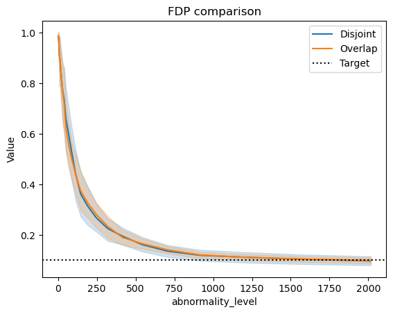
(a) mFDR, $\alpha=0.1$, $\pi=0.01$

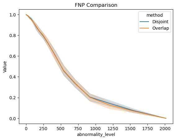
(b) FNR, $\alpha=0.1$, $\pi=0.01$

Figure 9: Comparison of mFDR and FNR control with disjoint and overlapping windows method.

Conclusion

The FDR control quality are similar for both strategies, overlapping windows and disjoint windows. This imply that performances of the anomaly detector to not decrease by using overlapping windows instead of disjoint windows. This is a practical result that allows to do real time detection without having to wait to complete disjoint windows.

4.4.3 Convergence of false discovery rate control

This section studies the convergence rate of the FDR over the full time series using $mBH_{\alpha}$.

Experiment Description

The theoretical results obtained in Theorem 4 only guarantee an asymptotic control of the FDR on the whole time series. In practice, it is more useful to have a control of the FDR at any time, i.e. on subseries of finite size. The question is empirically studied by observing the speed of convergence of the false discovery rate towards the level $\alpha$. The FDR of the full time series is calculated across different scenarios, as a function of time series size. In order to get the distribution of the FDR, the experiment is repeated on $B=100$ time series. The maximal time series size explored is $T=10^{4}$.

1. For $1\leq b\leq B$ and for $1\leq t\leq T$:

   • $A_{b,t}\sim Ber(\pi)$

   • If $A_{b,t}=0$, $p_{b,t}\sim U([0,1])$

   • Otherwise: $p_{b,t}\sim U([0,1/\delta])$

2. The thresholds are estimated with $mBH_{\alpha}$:

   $$\hat{\varepsilon}_{b,t,\alpha}=\hat{\varepsilon}_{mBH_{\alpha}}(p_{b,t-m+1},\ldots,p_{b,t})$$

3. The proportion of false discovery (FDP) on the partial time series are calculated:

   $$FDP_{b,t,\alpha}=\frac{\sum_{u=1}^{t}(1-A_{b,t})\mathbb{1}[p_{b,t}\leq\hat{\varepsilon}_{b,t,\alpha}]}{\sum_{u=1}^{t}\mathbb{1}[p_{b,t}\leq\hat{\varepsilon}_{b,t,\alpha}]}$$

Different scenarios are generated by varying the proportion of anomalies $\pi$ and the atypicity level $\delta$.

Results and analysis

In Figure 10, the false discovery proportion is represented in the ordinate according to the size of the time series given in the abscissa. The different levels of $\alpha$ used to compute $mBH$ threshold are experimented with the results of the median FDP and its 95% band is shown in different colors. Different scenarios are represented by varying the proportion of anomalies between the sub figures.

It can be observed that the convergence is quite fast from a size of 2000 data points, since for a $\alpha$ of 0.05, is has 95% chance to have a false positive rate between 0.04 and 0.06, on Figure 10. Thus, the control of the false positive rate, can be ensured with a high probability, for a series of one data point per minute recorded over a few days, .

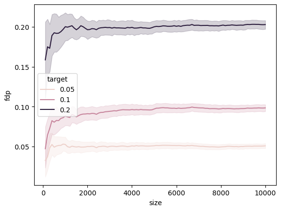
(a) $\delta=1000$, $\pi=0.02$

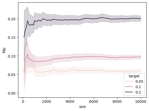
(b) $\delta=1000$, $\pi=0.01$

Figure 10: FDR over the full time series as a function of the time series size.

Conclusion

This ensures that the control at level is reached not only for infinite time series but also for finite time series which allows our model to be used in practice.

5 Empirical simulation against competitor

The control of the FDR with $p$-values estimated empirically has been studied at Section 3. Theorem 2 ensure the control of the $FDR_{1}^{m}$ when the $p$-values are estimated on calibration set having particular cardinality value. Theorems 3 and 4 ensure the control of the FDR of the full time series throw control of the $mFDR_{1}^{m}$ of the subseries. Corollary 5 enables to deduce that the $mBH_{\alpha}$ procedure can be apply to control the FDR of the full time series under the Heuristic and Power assumptions. Even though these assumptions are hard to ensure theoretically, the experiment at Section 4.4.1 shows that the $mFDR_{1}^{m}$ is controlled for tested scenario, provided that anomalies are sufficiently atypical. Experiment from Section 4.4.3 shows that the control of the FDR is possible even the time series is not infinite as required by Theorem 4.

These different results provide the conditions for building an anomaly detector that controls the FDR of the time series through control of the mFDR on the subseries and the $p$-empirical value. Our anomaly detector is evaluated under different scenarios by varying the generated anomalies and the targeted FDR. To understand the source of the difficulties that the anomaly detector may encounter, different sequences of $p$-values with oracle information are introduced. Our anomaly detector is compared against Levels based On Recent Discovery (LORD) which is a online multiple testing procedure, introduced in [30] to control the FDR.

5.1 Data

The synthetic data are generated from Gaussian distribution. With the use of the empirical $p$-value estimator there are no need to evaluate on other data distribution. Only anomaly proportion and the distribution shift associated to anomalies impact the performances of the anomaly detector. Data are generated accordingly with Definition 4 with Gaussian reference distribution and anomaly spike like in Section 3.4.1. The strength of the distribution shift noted by $\Delta$ takes value in $\{3\sigma,3.5\sigma,4\sigma\}$ and the abnormality proportion noted $\pi$ is equal to $0.01$. Each generated time series contain $T=10^{4}$ data points. Each experiment is repeated over $100$ time series.

For $t$ in $\llbracket 1,T\rrbracket$:

• $A_{t}\sim B(\pi)$

• $X_{t}=\begin{cases}\mathcal{N}(0,\sigma^{2})&\text{if }A_{t}=0\\ \Delta\sigma&\text{else}\end{cases}$

The value of $\Delta$ represents the atypicity score of the anomalies. Anomalies with higher $\Delta$ are easier to detect. In this experiment, the standard deviation $\sigma$ is set to 1.

5.2 Threshold and $p$-value estimators description

5.2.1 Our proposal mBH on overlapping subseries

Using the $p$-value with the empirical estimator, the anomalies are detected by using mBH as the threshold estimator on overlapping subseries in the Algorithm 1. For each time $t$, the threshold is computed as: $\hat{\varepsilon}_{mBH_{\alpha},t}=f_{m}(\hat{p}_{t-m},\ldots,\hat{p}_{t})$, where $f_{m}$ is the mBH-procedure. To ensure FDR control according to Theorem 1, the cardinality of the calibration set to be equal to $n=\frac{m}{\alpha}-1$. In this experiment $m$ is equal to $100$ and $\alpha$ takes values $0.1$ and $0.2$ depending the tested scenario. So the calibration set takes values $999$ or $1999$.

5.2.2 LORD

LORD introduced in [30] is based on alpha-investing rules to define a threshold on $p$-values. For each time $t$ the threshold is computed from according to the alpha-investing rules, depending on previous decision made by the algorithm. For more precision refer to the original article [30]. The empirical $p$-value specified in Definition 2.4 does not respect this property while the conformal $p$-value, defined in Equation 2.5 respects this property. Using conformal $p$-values to apply LORD algorithm leads to a weak power detecting anomalies. The issue is that $\tilde{p}\geq\frac{1}{n+1}$ is always verified and the threshold sequence $\hat{\varepsilon}_{t}$ decreases quickly when no rejection are made. No anomaly can be detected. For these reasons, the empirical $p$-value introduced in Equation 2.4 is used while applying LORD and mBH. In this experiment LORD3 from [30] is used with the same parameters as in the original paper.

5.2.3 $p$-value estimation

Different sequences of $p$-values are used to understand the limitations of our anomaly detector. The true $p$-values are used to evaluate the case where the only limitation comes from the multiple testing procedure. One can thus understand how the estimation of the $p$-values affects the detection of anomalies. One way to estimate $p$-values in practice is to use the same calibration set for all $p$-values. This is referred as the fixed calibration set. However, the $p$-values may be biased in that particular calibration set. In practice, the usual way to implement the estimated $p$-values is to use a sliding calibration set. To evaluate the $p$-value of a data point $X_{t}$, $n$ preceding data points are used as a calibration set. To a bias in the estimation, the points detected as abnormal cannot be part of the calibration set. However, the calibration set can be biased by undetected anomalies. To evaluate this impact, the sliding calibration set-$\star$ is introduced, where the knowledge oracle of the labels is used to construct the calibration set from the previous data points.

The different $p$-value sequences are computed as follows:

• Oracle: The true $p$-value is used instead of the estimated one.

  $$\forall t\in\llbracket 1,T\rrbracket,\hat{p}_{t}=\Phi(X_{t})$$

• Fixed calibration set (Fixed Cal.): The $p$-value is estimated using the same calibration set $\{Z_{i},i\in[1,n]\}$ for all observations.

  $$\forall t\in\llbracket 1,T\rrbracket,\hat{p}_{t}=\frac{1}{n}\sum_{i=1}^{n}\mathbb{1}[Z_{i}>X_{t}]$$

• Sliding Calibration set-$\star$ (Sliding Cal.-$\star$): The $p$-value is estimated using a calibration that is a sliding windows containing the $n$ previous true normal data.

  $$\forall t\in\llbracket 1,T\rrbracket,\hat{p}_{t}=\frac{1}{n}\sum_{i=1}^{n}\mathbb{1}[X_{h(t,i)}>X_{t}]$$

  With $h$ the function that select observation that respect $\mathcal{H}_{0}$. For each $t$ and $i$, $h(t,i)$ gives the $i$-th observation lower than $t$ and that respect $\mathcal{H}_{0}$ hypothesis.

• Sliding Calibration set (Sliding Cal.): The calibration set is a sliding windows containing the $n$ previous estimated normal data.

  $$\forall t\in\llbracket 1,T\rrbracket,\hat{p}_{t}=\frac{1}{n}\sum_{i=1}^{n}\mathbb{1}[X_{\hat{h}(t,i)}>X_{t}]$$

  With $\hat{h}$ the function that estimates the function $h$. For each $t$ and $i$, $\hat{h}(t,i)$ give the $i$-th observation lower than $t$ and $d_{\hat{h}(t,i)}=0$.

5.3 Performance metrics

The anomaly detector are evaluated using their ability to control the FDR and minimize the FNR of the full time series. Therefore, the two applied metrics are the FDP and the FNP computed as:

$$FDP=\frac{\sum_{t=1}^{T}\mathbb{1}[\hat{p}_{t}<\hat{\varepsilon}_{t}](1-A_{t})}{\sum_{t=1}^{T}\mathbb{1}[\hat{p}_{t}<\hat{\varepsilon}_{t}]}$$

and

$$FNP=\frac{\sum_{t=1}^{T}\mathbb{1}[\hat{p}_{t}<\hat{\varepsilon}_{t}](1-A_{t})}{\sum_{t=1}^{T}A_{t}}$$

where $\hat{\varepsilon}_{t}$ is estimated using mBH or LORD and $\hat{p}_{t}$ is estimated using one of the estimator defined in Section 5.2.3.

5.4 Results

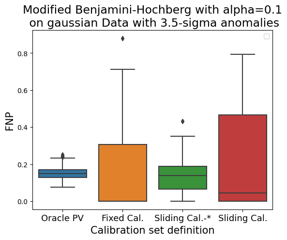
(c) mBH, $3.5-$sigma

(d) LORD, $3.5-$sigma

(e) mBH, $3-$sigma

(f) LORD, $3-$sigma

Figure 16: Comparison of the FNPs acquired from using different multiple testing procedures, mBH or LORD, and from the way the $p$-values are calculated, in the case $\alpha=0.1$.

The box plots shown in Figures 15-18 represent the FDP and FNP distribution for 1000 repetitions. Inside each sub figure (a, b, c, d, e,..), the box plot distributions are displayed according to:

1. the multiple testing method mBH or LORD,

2. the $p$-value estimation model set to Oracle PV, Fixed Cal., Sliding Cal.-$\star$ or Sliding Cal.

3. and the distribution shift between the normal data and anomalies, noted $\Delta$, varying from $4\sigma$ to $3\sigma$.

Table 4 gives a summary using FDR and FNR estimations. It enables easily the comparison between these values coming from the different strategies combining:

1. the multiple testing method mBH or LORD,

2. the choice of the level $\alpha$ varying from $0.1$ to $0.2$,

3. the $p$-value estimation model set to Oracle PV, Fixed Cal., Sliding Cal.-$\star$ or Sliding Cal.

4. and the distribution shift between the normal data and anomalies, varying from $4\sigma$ to $3\sigma$.

FDR, $\alpha=0.1$	$\Delta=4\sigma$	$\Delta=3.5\sigma$	$\Delta=3\sigma$
mBH with Oracle PV	0.101	0.113	0.281
mBH with Fixed Cal.	0.100	0.109	0.348
mBH with Sliding Cal.-$\star$	0.100	0.113	0.256
mBH with Sliding Cal.	0.335	0.222	0.346
LORD with Oracle PV	0.106	0.115	0.367
LORD with Fixed Cal.	0.111	0.277	0.736
LORD with Sliding Cal.-$\star$	0.070	0.190	0.841
LORD with Sliding Cal.	0.075	0.098	0.627

(a) FDR, $\alpha=0.1$

FNR, $\alpha=0.1$	$\Delta=4\sigma$	$\Delta=3.5\sigma$	$\Delta=3\sigma$
mBH with Oracle PV	0.020	0.151	0.793
mBH with Fixed Cal.	0.026	0.135	0.669
mBH with Sliding Cal.-$\star$	0.019	0.140	0.669
mBH with Sliding Cal.	0.040	0.217	0.694
LORD with Oracle PV	0.033	0.260	0.905
LORD with Fixed Cal.	0.070	0.340	0.896
LORD with Sliding Cal.-$\star$	0.781	0.845	0.978
LORD with Sliding Cal.	0.052	0.327	0.907

(b) FNR, $\alpha=0.1$

FDR, $\alpha=0.2$	$\Delta=4\sigma$	$\Delta=3.5\sigma$	$\Delta=3\sigma$
mBH with Oracle PV	0.200	0.208	0.277
mBH with Fixed Cal.	0.206	0.211	0.301
mBH with Sliding Cal.-$\star$	0.210	0.219	0.283
mBH with Sliding Cal.	0.833	0.815	0.761
LORD with Oracle PV	0.211	0.216	0.290
LORD with Fixed Cal.	0.210	0.263	0.665
LORD with Sliding Cal.-$\star$	0.061	0.149	0.625
LORD with Sliding Cal.	0.117	0.133	0.321

(c) FDR, $\alpha=0.2$

FNR, $\alpha=0.2$	$\Delta=4\sigma$	$\Delta=3.5\sigma$	$\Delta=3\sigma$
mBH with Oracle PV	0.009	0.062	0.395
mBH with Fixed Cal.	0.014	0.045	0.355
mBH with Sliding Cal.-$\star$	0.008	0.059	0.339
mBH with Sliding Cal.	0.003	0.018	0.101
LORD with Oracle PV	0.016	0.117	0.610
LORD with Fixed Cal.	0.04	0.144	0.689
LORD with Sliding Cal.-$\star$	0.805	0.835	0.941
LORD with Sliding Cal.	0.026	0.168	0.692

(d) FNR, $\alpha=0.2$

Table 4: Comparison of mBH versus LORD for online anomaly detection in Gaussian white noise with different abnormality levels.

5.5 Analysis

5.5.1 Effect of the strength of the distribution shift $\Delta$

According the assumption Power from Theorem 5, $mBH_{\alpha}$ enables control of the FDR at level $\alpha$ if all anomalies are detected.
To test this assertion, the different columns of the Table 4(a), are compared. In the row “mBH with Oracle PV”, with $\Delta=4\sigma$ the FDR is estimated at $0.101$ which is close to the desired level $\alpha=0.1$. While, when $\Delta=3\sigma$ the FDR level is estimated at $0.281$ which is almost three times the desired level $\alpha$. The FNR results in Table 4(b) needs to be taken into consideration. When $\Delta=4\sigma$, the FNR is close to 0, while when $\Delta=3\sigma$ the FNR is equal to $0.793$. Similar results are obtained with other test configurations in Table 4(c) and Table 4(d). The FDR control at the desired level need the FNR to be close to 0.

5.5.2 Effect of $p$-value estimation

To understand how the $p$-value estimation can prevent the control of the FDR, the first four rows in Table 4(a) are compared. In the column “$4\sigma$”, the FDR values for the configurations “Oracle PV”, “Fixed Cal.” and “Sliding Cal.-$\star$” are very close to the desired level $\alpha=0.1$. This control is enabled by Theorem 5, since the $p$-values verify all hypotheses, in particular all data in the calibration sets are generated according to the reference distribution. However, in the case of “Sliding Cal.”, the FDR increases at a value of $0.335$. For the same configurations, the FDR remains low, between $0.019$ and $0.040$ as shown at Table 4(b). The increase of FDR when using “Sliding Cal.” instead of “Sliding Cal.-$\star$” is a consequence of calibration set contamination. Indeed, according to the procedure used to build the calibration sets, described in Section 5.2.3, all detected anomalies are removed from calibration sets used in the estimation of next $p$-values. When an observation is wrongly detected as an anomaly, this data point cannot be part of the calibration set at future steps of the online detection. Instead, it is replaced by an other data point having statistically a lower atypicity score. Indeed false positives have high atypicity score to be (wrongly) detected as anomalies. As a result, the calibration set contains data points with lower scores than if it had been generated under $\mathcal{P}_{0}$. It leads to underestimate the $p$-values and to increase the number of false positives. This illustrates the major drawback of mBH: it is highly sensitive to the non robustness of the $p$-value estimator. Figure 15(a) shows that using fixed calibration instead of sliding calibration-$\star$ gives a larger variance on the FDP while the FDR is the same. Using a single calibration set for the entire time series means that the FDP is highly dependent on the start of the time series. By modifying the calibration set at each time step, the statistical fluctuations in the FDP are smoothed over the course of the time series analysis.

5.5.3 Comparison with LORD

In this section, the results found using mBH and the ones using LORD are compared. As known from the literature, LORD controls the FDR of super-uniform $p$-values. In this experiment, the question is in the capacity of LORD method to control the FDR of empirical $p$-values that have no theoretical guaranties. It can be noticed in Figure 4(a) that LORD is able to ensure the control of the FDR for all calibration set definitions when anomalies are easier to detect as for $\Delta=4\sigma$ or $\Delta=3.5\sigma$. In particular, unlike mBH, LORD is able to control the FDR in the case of the sliding calibration set. However, mBH method has a lower FNR compared to the LORD method, as shown in 4(a) and 4(b). For example, Table 4(b) shows that the FNR is equal to $0.019$ with mBH while it is equal to $0.781$ with LORD, in the case using Sliding Calibration set-$\star$ on data having $\Delta=3\sigma$. Nevertheless, with the Sliding Calibration set case, the LORD method has quite the same FNR but with lower FDR ($0.335$ against $0.075$). The contamination issue of mBH offsets the superior performance observed in the Sliding Calibration set-$\star$.

6 Conclusion

In this article, an online anomaly detector that aims to have a better control of the FDR at a given level $\alpha$ has been proposed. The research has been developed to tackle two issues:

• the empirical $p$-values: it ensures conditions on the calibration cardinality to ensure FDR control when using Benjamini-Hochberg.

• and the online detection: it ensures a global control of the FDR through local control of the mFDR of subseries, using a modified version of the BH-procedure.

The results of our research is the assessment of our proposal from the theoretical point of view and from empirical experiments. Our method has been compared with a method from the state of the art. It shows the strong capability for ensuring control of the FDR even in the case of empirical $p$-values. The major drawback and improvement path of our method is it relies on non-robust $p$-value estimation.

7 Acknowledgments

The authors would like to thank Cristian Preda, director of the MODAL team at Inria, for valuable discussions.

Appendix A Proofs

A.1 Comparison of $p$-values estimators

The control of the FDR is not achievable using classical multiple testing [6, 49] since the $p$-value estimator, shown in Definition 2, is not super-uniform. Conformal $p$-value estimator $\tilde{p}$, shown in Equation 2.5, verifies the super-uniform property. However, this estimator $\tilde{p}\geq\frac{1}{m+1}$ has lower power because zero anomalies are detected with thresholds below $\frac{1}{m+1}$.

Figure 11 displays the comparison between estimated $p$-values and conformal $p$-values using the BH-procedure. As shown in Figure 11(a), the conformal $p$-values ensure an upper bound on the FDR at level $\frac{m_{0}}{m}\alpha$, while the estimated $p$-values ensure only a lower bound at the same level. Moreover, perfect control are reached for $n=1000$ and $n=2000$ with conformal $p$-values while the control is reached for $n=999$ and $n=1999$ with estimated $p$-values. As shown in Figure 11(b), the FNR for conformal $p$-values estimator is always larger than the one for estimated $p$-values. However for the $n$ points that control the FDR, the FNR values are close.

To conclude, the choice between conformal $p$-values and estimated $p$-values depends on the calibration set size. Indeed, for calibration set $n=1000$ the performances are similar. But for other calibration set sizes as $n=1500$ the FDR control are similar but the FNR is better for estimated $p$-values.

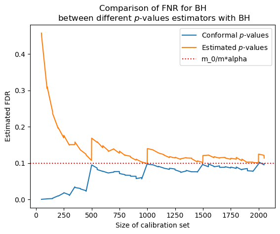
(a) FDR

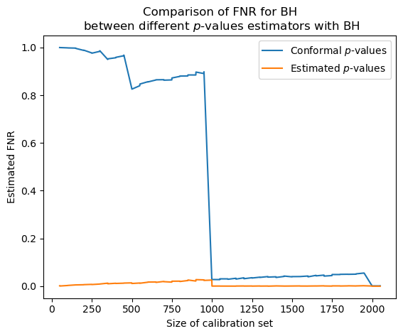
(b) FNR

Figure 11: Comparison between $p$-value estimators using Benjamini-Hochberg

A.2 PRDS property for $p$-values having overlapping calibration set

The following construction is used to describe a family of $p$-values with overlapping calibration set. Let $Z$ the vector that combine all calibration set, the $Z_{i}$ are i.i.d. with marginal probability $\mathcal{P}_{0}$. The set of the $n$ indices defining the elements of the calibration set related to $\hat{p}_{i}$ in $Z$ is noted $\mathcal{D}_{i}$. The calibration related to $X_{1}$ is noted $Z_{\mathcal{D}_{1}}=(Z_{i_{1}},\ldots,Z_{i_{n}})$. For all $i$ in $\llbracket 1,m\rrbracket$: $\hat{p}_{i}=p\mbox{-value}(X_{i},Z_{\mathcal{D}_{i}})$.

To proof that $p$-values with overlapping calibration set are PRDS as described in Definition 1, the methodology used in [4] to be extended in the case of overlapping calibration set. For $i$ in $\llbracket 1,m\rrbracket$ the calibration set associated to $X_{i}$ is noted $Z_{\mathcal{D}_{i}}$. The law of total probabilities gives:

$$\mathbb{P}\left[\hat{p}_{1}^{m}\in A|\hat{p}_{i}=u\right] =\int\mathbb{P}\left[\hat{p}_{1}^{m}\in A|\hat{p}_{i}=u|Z_{\mathcal{D}_{i}}=z\right]\mathbb{P}\left[Z_{\mathcal{D}_{i}}=z\right|]dz$$

$$=\mathbb{E}_{Z_{\mathcal{D}_{i}}|\hat{p}_{i}=u}\mathbb{P}\left[\hat{p}_{1}^{m}\in A|\hat{p}_{i}=u|Z_{\mathcal{D}_{i}}=z\right]$$

If these two lemma are suppose to be true, the PRDS property is verified.

Lemma 5.1.

For non-decreasing set $A$ and vectors $z$, $z^{\prime}$ such that $z\succeq z^{\prime}$, then

$$\mathbb{P}\left[\hat{p}_{1}^{m}\in A|Z_{\mathcal{D}_{i}}=z\right]\geq\mathbb{P}\left[\hat{p}_{1}^{m}\in A|Z_{\mathcal{D}_{i}}=z^{\prime}\right]$$ (A.1)

Lemma 5.2.

For $u\geq u^{\prime}$, if $i$ belongs to the set of inliers, the exists $Z_{{\mathcal{D}_{i}},1}\sim Z_{\mathcal{D}_{i}}|\hat{p}_{i}=u$ and $Z_{{\mathcal{D}_{i}},2}\sim Z_{\mathcal{D}_{i}}|\hat{p}_{i}=u^{\prime}$ such that $\mathbb{P}[Z_{{\mathcal{D}_{i}},1}]\succeq\mathbb{P}[Z_{{\mathcal{D}_{i}},2}]$

Indeed, take $i\in\llbracket 1,m\rrbracket$ and $u\geq u^{\prime}$ and define $Z_{{\mathcal{D}_{i}},1}$ and $Z_{{\mathcal{D}_{i}},2}$ as in the statement of Lemma 5.2.

$$\mathbb{P}[\hat{p}_{1}^{m}\in A|p_{i}=u] =\mathbb{E}_{Z_{{\mathcal{D}_{i}},1}}[\mathbb{P}[\hat{p}_{1}^{m}\in A|Z_{\mathcal{D}_{i}}=Z_{{\mathcal{D}_{i}},1}]]\text{ (Lemma \ref{lemma:z1z2})}$$

$$\geq\mathbb{E}_{Z_{{\mathcal{D}_{i}},2}}[\mathbb{P}[\hat{p}_{1}^{m}\in A|Z_{\mathcal{D}_{i}}=Z_{{\mathcal{D}_{i}},2}]]\text{ (Lemma \ref{lemma:pz})}$$

$$\geq\mathbb{P}[\hat{p}_{1}^{m}\in A|p_{i}=u^{\prime}]\text{ (Lemma \ref{lemma:z1z2})}$$

It shows that, when $u\geq u^{\prime}$ then $\mathbb{P}[\hat{p}_{1}^{m}\in A|p_{i}=u]\geq\mathbb{P}[\hat{p}_{1}^{m}\in A|p_{i}=u^{\prime}]$, which means $\mathbb{P}[\hat{p}_{1}^{m}\in A|p_{i}=u]$ is increasing in $u$. The PRDS property is satisfied. To complete the proof, the introduced lemmas are proven.

Proof of Lemma 5.1.

Let be $i$ in $\llbracket 1,m\rrbracket$ and vectors $z$, $z^{\prime}$ and $\overline{z}$ vectors such that $z\succeq z^{\prime}$. The vectors $z$, $z^{\prime}$ are used to define the calibration set related to the $p$-values $\hat{p}_{i}$ and $\overline{z}$ is used to define elements of calibrations sets that are not in the calibration set of $\hat{p}_{i}$. By conditioning on the calibration sets defined by $(z,\overline{z})$ and $(z^{\prime},\overline{z})$ it gives:

$$\mathbb{P}\left[\hat{p}_{1}^{m}\in A|Z_{\mathcal{D}_{i}}=z,Z_{\overline{\mathcal{D}_{i}}}=\overline{z}\right]\geq\mathbb{P}\left[\hat{p}_{1}^{m}\in A|Z_{\mathcal{D}_{i}}=z^{\prime},Z_{\overline{\mathcal{D}_{i}}}=\overline{z}\right]$$ (A.2)

This result comes from the decomposition the following decomposition, for all $j$ in $\llbracket 1,m\rrbracket$

$$\hat{p}_{j} =\frac{1}{n}\sum_{k\in\mathcal{D}_{j}}\mathbb{1}[a(Z_{k})\geq a(X_{j})]$$

$$=\frac{1}{n}\left(\sum_{k\in\mathcal{D}_{j}\cap\mathcal{D}_{i}}\mathbb{1}[a(Z_{k})\geq a(X_{j})]+\sum_{k\in\mathcal{D}_{j}\setminus\mathcal{D}_{i}}\mathbb{1}[a(Z_{k})\geq a(X_{j})]\right)$$

The conclusion comes from $Z_{\mathcal{D}_{i}}\succeq Z^{\prime}_{\mathcal{D}_{i}}$ which implies $Z_{\mathcal{D}_{i}\cap\mathcal{D}_{j}}\succeq Z^{\prime}_{\mathcal{D}_{i}\cap\mathcal{D}_{j}}$.

Since $Z_{\mathcal{D}_{j}\setminus\mathcal{D}_{i}}\perp Z_{\mathcal{D}_{i}}$, Eq. A.2 can be integrated over $Z_{\overline{\mathcal{D}_{i}}}$ to give:

$$\mathbb{P}\left[\hat{p}_{1}^{m}\in A|Z_{\mathcal{D}_{i}}=z\right]\geq\mathbb{P}\left[\hat{p}_{1}^{m}\in A|Z_{\mathcal{D}_{i}}=z^{\prime}\right]$$ (A.3)

∎

Proof of Lemma 5.2.

Let $S^{\prime}_{i,(1)}\leq S_{i,(2)}\leq\ldots\leq S_{i,(n)}$ the order statistics of $(a(Z_{{\mathcal{D}_{i}},1}),\ldots,a(Z_{{\mathcal{D}_{i}},n}))$. Let $S^{\prime}_{i,(1)}\leq S^{\prime}_{i,(2)}\leq\ldots\leq S^{\prime}_{i,(n+1)}$ the order statistics of $(a(Z_{{\mathcal{D}_{i}},1}),\ldots,a(Z_{{\mathcal{D}_{i}},n}),a(X_{i}))$. And $R_{i}$ the rank of $a(X_{i})$ among these.

$$\left\{(S_{(1)},\ldots,S_{(n)})|R_{i}=k,S^{\prime}_{i,(1)},\ldots,S^{\prime}_{i,(n+1)}\right\}=(S^{\prime}_{(1)},\ldots,S^{\prime}_{(k-1)},S^{\prime}_{(k+1)},\ldots,S^{\prime}_{(n+1)})$$ (A.4)

Using that $R_{i}$ is independent of $S^{\prime}_{i,(1)},\ldots,S^{\prime}_{i,(n+1)}$:

$$\left\{(S_{(1)},\ldots,S_{(n)})|R_{i}=k\right\}=(S^{\prime}_{(1)},\ldots,S^{\prime}_{(k-1)},S^{\prime}_{(k+1)},\ldots,S^{\prime}_{(n+1)})$$ (A.5)

The right-hand side is not increasing with $k$ and $\hat{p}_{i}=\frac{R_{i}-1}{n}$ ∎

A.3 Proof of Theorem 1

Proof of Theorem 1.

Let $R$ be a random variable describing the number of rejections made by $BH_{\alpha}$ that is, $R=\sum_{i=1}^{m}D_{i}$, where $D_{i}=1$ if hypothesis $\mathcal{H}_{0,i}$ is rejected. Let also $FP$ be the number of false positives made by $BH_{\alpha}$. Then, $FP=\sum_{i=1}^{m}A_{i}D_{i}=\sum_{i=1}^{m_{0}}D_{i}$, where $A_{i}$ is a random variable equal to 1 if hypothesis $\mathcal{H}_{0,i}$ is true and 0 otherwise. Furthermore

$$FDP=\frac{FP}{R} =\sum_{i=1}^{m_{0}}\frac{\mathbb{1}[p_{i}\leq\frac{\alpha R}{m}]}{R}\quad\qquad\mbox{(since $D_{i}=\mathbb{1}[p_{i}\leq\frac{\alpha R}{m}]$)}$$

$$=\sum_{k=1}^{m}\sum_{i=1}^{m_{0}}\frac{\mathbb{1}[p_{i}\leq\frac{\alpha k}{m}]\mathbb{1}[R=k]}{k}.$$ (A.6)

Let us now introduce the random variables $R(i)$ that are the number of rejections generated by BH when $p_{i}$ is replaced by the value $0$ that is, $R(i)=BH_{\alpha}(p_{1},..,p_{i-1},0,p_{i+1},\ldots,p_{m})$. It results that

$$\mathbb{1}[p_{i}\leq\frac{\alpha k}{m}]\mathbb{1}[R=k]=\mathbb{1}[p_{i}\leq\frac{\alpha k}{m}]\mathbb{1}[R(i)=k],$$

since, on the event $\{p_{i}\leq\frac{\alpha k}{m}\}$, $p_{i}$ is rejected and therefore $R=R(i)$. Let us also notice that the independence between the $p$-values is already used at this stage since modifying the value of $p_{i}$ does not affect that of the others.

By combining the previous argument and the independence between $R(i)$ and the other $p$-values, the expectation on both sides yields

$$FDP =\sum_{k=1}^{m}\sum_{i=1}^{m_{0}}\frac{\mathbb{1}[p_{i}\leq\frac{\alpha k}{m}]\mathbb{1}[R(i)=k]}{k}$$

$$\Rightarrow\quad FDR=\mathbb{E}[FDP] =\sum_{k=1}^{m}\sum_{i=1}^{m_{0}}\frac{\mathbb{P}[p_{i}\leq\frac{\alpha R}{m}]\mathbb{P}[R(i)=k]}{k}$$

$$=\sum_{k=1}^{m}\sum_{i=1}^{m_{0}}\frac{\frac{\alpha k}{m}\mathbb{P}[R(i)=k]}{k}$$

$$=\frac{m_{0}\alpha}{m},$$

where the last equality results from the fact that the true $p$-values follow a uniform distribution on $[0,1]$. The result finally follows from noticing that for each $1\leq i\leq m_{0}$, $\sum_{k=1}^{m}\mathbb{P}[R(i)=k]$, since $R(i)\geq 1$ by definition. ∎

A.4 Proof of Corollary 1

Proof of Corollary 1.

To get a deeper understanding of the FDR expression obtained in Theorem 2, $q_{n,k}$ the fractional part of $\frac{\alpha kn}{m}$ is introduced:

$$q_{n,k}=\frac{\alpha kn}{m}-\left\lfloor\frac{\alpha kn}{m}\right\rfloor$$

When plugged into the FDR expression, it gives:

$$FDR=m_{0}\sum_{k=1}^{m}\frac{\frac{\frac{\alpha kn}{m}+1-q_{n,k}}{n+1}}{k}\mathbb{P}(R(1)=k)$$

$$FDR=\frac{m_{0}\alpha}{m}\frac{n}{n+1}+\frac{m_{0}}{n+1}\sum_{k=1}^{m}\frac{1-q_{n,k}}{k}\mathbb{P}(R(1)=k)$$ (A.7)

In order to get lower and upper bounds of the FDR, the value of $q_{n,k}$ should be expressed as a function of $\alpha$, $k$, $n$ and $m$.

For the next part of the proof, it is useful to express the relation between $q_{n,k}$ and $q_{n+1,k}$. It gives the effect of increasing the cardinality of the calibration by one. Using the definition of the fractional part:

$$q_{n+1,k}-q_{n,k} =\frac{\alpha k(n+1)}{m}-\left\lfloor\frac{\alpha k(n+1)}{m}\right\rfloor-\frac{\alpha kn}{m}+\left\lfloor\frac{\alpha kn}{m}\right\rfloor$$

$$q_{n+1,k}-q_{n,k} =\frac{\alpha k}{m}-\left\lfloor\frac{\alpha k(n+1)}{m}\right\rfloor+\left\lfloor\frac{\alpha kn}{m}\right\rfloor$$

Which can be expressed as a congruence relation:

$$q_{n+1,k}-q_{n,k}\equiv\frac{\alpha k}{m}\pmod{1}$$ (A.8)

Two cases are studied:

1. Particular case: there exists an integer $1\leq\ell$ such that $\frac{\ell m}{\alpha}$ is an integer. the notation $n_{\ell}=\frac{\ell m}{\alpha}$ is introduced. Since: $\frac{\alpha kn_{\ell}}{m}=\frac{\alpha k\ell m/\alpha}{m}=k\ell$ is an integer, then the fractional part is null:

   $$q_{n_{\ell},k}=0$$

   If the calibration set cardinality $n$ is equal to $n=n_{\ell}-1=\frac{\ell m}{\alpha}-1$. Then, the congruence relation in Eq. A.8 gives:

   $$q_{n_{\ell}-1,k}\equiv q_{n_{l},k}-\alpha k/m\pmod{1}$$

   $$q_{n_{\ell}-1,k}\equiv 0-\alpha k/m\pmod{1}$$

   Using the fact that fractional part of a number belongs to $[0,1[$, the only possible value to $q_{n_{\ell}-1,k}$ is:

   $$q_{n_{\ell}-1,k}=1-\alpha k/m$$

   Plugging the value of $q_{n_{\ell}-1,k}$ into Eq. A.7, it gives:

   $$FDR =\frac{m_{0}\alpha n}{m(n+1)}+\frac{m_{0}}{n+1}\sum_{k=1}^{m}\frac{\alpha k}{km}\mathbb{P}(R(1)=k)$$

   Simplifying by $k$ and using that $\sum_{k=1}^{m}\mathbb{P}(R(i)=k)=1$, the result is obtained:

   $$FDR =\frac{m_{0}\alpha n}{m(n+1)}+\frac{m_{0}\alpha}{(n+1)m}$$

   $$FDR =\frac{m_{0}\alpha}{m}$$

2. General case: With $\alpha\in]0,1]$, for each $\ell$ the notation $n_{\ell}=\left\lceil\frac{\ell m}{\alpha}\right\rceil$ is introduced. Notice that this definition is consistent with the particular case. The ceiling function definition gives:

   $$\left\lceil\frac{\ell m}{\alpha}\right\rceil-1<\frac{\ell m}{\alpha}\leq\left\lceil\frac{\ell m}{\alpha}\right\rceil$$

   Multiplying by $\alpha k$ on each side and the $n_{\ell}$ notation:

   $$\frac{\alpha k(n_{\ell}-1)}{m}<k\ell\leq\frac{\alpha k(n_{\ell})}{m}$$

   It implies that $\lfloor\frac{\alpha k(n_{\ell}-1)}{m}\rfloor<\lfloor\frac{\alpha k(n_{\ell})}{m}\rfloor$. Also, Eq. A.8 is expressed as $q_{n_{\ell},k}-q_{n_{\ell}-1,k}\equiv\frac{\alpha k}{m}\pmod{1}$:

   $$1-\frac{\alpha k}{m}\leq q_{n_{\ell}-1,k}<1$$ (A.9)

   Indeed, the fractional part of a number as to be larger than $1-\alpha k/m$ so that adding $\alpha k/m$ increase the integer part.

   By plugin the bounds of $q_{n_{\ell}-1,k}$ into Eq. A.7, it can gives the bounds of the FDR. At first, to compute the upper bound of the FDR the lower bound of $q_{n_{\ell}-1,k}$ is used:

   $$FDR\leq\frac{m_{0}(n_{\ell}-1)\alpha}{mn_{\ell}}+\frac{m_{0}}{n+1}\sum_{k=1}^{m}\frac{\alpha k}{km}\mathbb{P}(R(1)=k)$$

   With the same calculations as for the “Particular case”, it gives:

   $$FDR\leq\frac{m_{0}\alpha}{m}$$

   Similarly, the lower bound of the FDR can be obtained using the $q_{n,k}$ upper bound from Eq. A.9 plugged into Eq. A.7:

   $$\frac{m_{0}(n_{\ell}-1)\alpha}{mn_{\ell}}+\frac{m_{0}}{n+1}\sum_{k=1}^{m}\frac{(1-1)}{k}\mathbb{P}(R_{1}=k)<FDR$$

   $$\frac{m_{0}(n_{\ell}-1)\alpha}{mn_{\ell}}<FDR$$

∎

A.5 Proof of Proposition 4

Proof of Proposition 4.

By definition $mFDR_{1}^{m}=\frac{\mathbb{E}[FP_{1}^{m}]}{\mathbb{E}R_{1}^{m}}$, and $R_{1}^{m}=FP_{1}^{m}+TP_{1}^{m}$. With hypothesis the $mFDR$ is equal to $\alpha$, this gives:

$$\alpha =\frac{\mathbb{E}[FP_{1}^{m}]}{\mathbb{E}R_{1}^{m}}$$

$$\alpha =\frac{\mathbb{E}[FP_{1}^{m}]}{\mathbb{E}[FP_{1}^{m}+TP_{1}^{m}]}$$

$$\alpha(\mathbb{E}[FP_{1}^{m}]+\mathbb{E}[TP_{1}^{m}]) =\mathbb{E}[FP_{1}^{m}]$$

$$(\alpha-1)\mathbb{E}[FP_{1}^{m}] =-\alpha\mathbb{E}[TP_{1}^{m}]$$

$$\mathbb{E}[FP_{1}^{m}] =\frac{\alpha}{1-\alpha}\mathbb{E}[TP_{1}^{m}]$$

Then, the expectation of true positives is expressed using the proportion of false negatives $\beta$, the proportion of anomaly $\pi$ in the $m$ observations, $A_{i}$ the random variable equal to $1$ if the observation $X_{i}$ is an anomaly and $D_{i}$ the random variable equal to $1$ if the observation $X_{i}$ is detected as anomaly :

$$\mathbb{E}[TP_{1}^{m}] =\sum_{i=1}^{m}\mathbb{P}[A_{i}=1\mbox{ and }D_{i}=1]$$

$$=\sum_{i=1}^{m}\mathbb{P}[A_{i}=1]\mathbb{P}[D_{i}=1|A_{i}=1]$$

$$=m\pi(1-\beta)$$

Therefore, the $\mathbb{E}[FP_{1}^{m}]$ can be expressed as:

$$\mathbb{E}[FP_{1}^{m}]=\frac{\alpha m\pi(1-\beta)}{1-\alpha}$$

So the $\mathbb{E}[R_{1}^{m}]$ is expressed as follows:

$$\mathbb{E}[R_{1}^{m}] =\frac{\alpha m\pi(1-\beta)}{1-\alpha}+m\pi(1-\beta)$$

$$=\frac{m\pi(1-\beta)}{1-\alpha}$$

∎

Appendix B Figures

B.1 Effect of the number detections by BH on the intermediate drops for the FDR control in Section 3.4

B.2 Figures related to experiment of Section 4.4.1

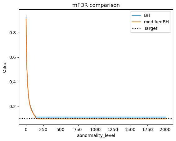
(a) mFDR, $\alpha=0.1$, $\pi=0.07$

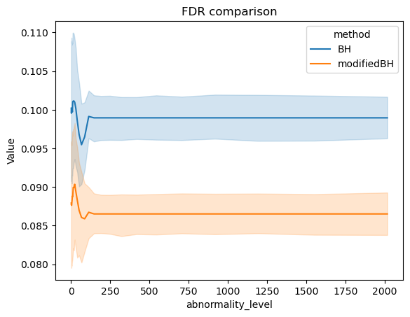
(b) FDR, $\alpha=0.1$, $\pi=0.07$

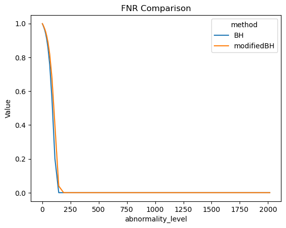
(c) FNR, $\alpha=0.1$, $\pi=0.07$

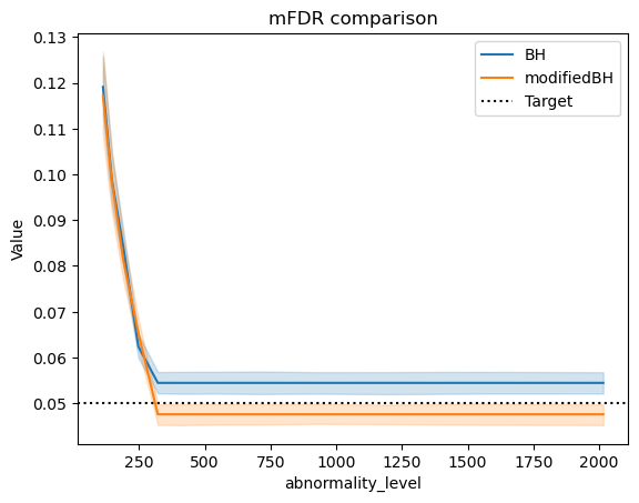
(d) mFDR, $\alpha=0.05$, $\pi=0.07$

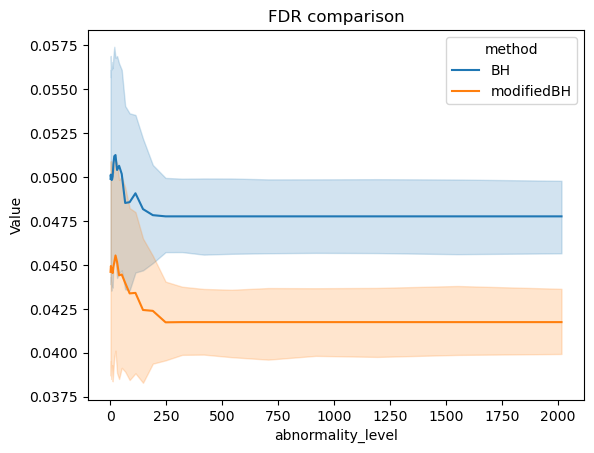
(e) FDR, $\alpha=0.05$, $\pi=0.07$

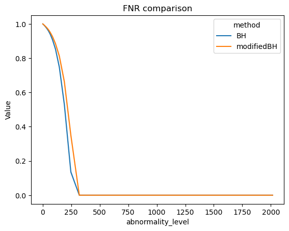
(f) FNR, $\alpha=0.05$, $\pi=0.07$

(g) mFDR, $\alpha=0.2$, $\pi=0.07$

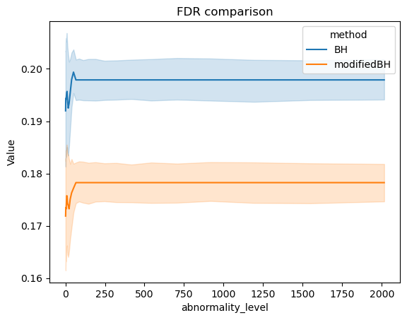
(h) FDR, $\alpha=0.2$, $\pi=0.07$

(i) FNR, $\alpha=0.2$, $\pi=0.07$

(j) mFDR, $\alpha=0.1$, $\pi=0.01$

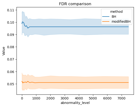
(k) FDR, $\alpha=0.1$, $\pi=0.01$

(l) FNR, $\alpha=0.1$, $\pi=0.01$

Figure 13: Effect of the atypicity level on the mFDR, FDR and FNR, according to different multiple testing procedures.

B.3 Figures related to experiment of Section 4.4.1

(a) mFDR, $\alpha=0.1$, $\pi=0.01$

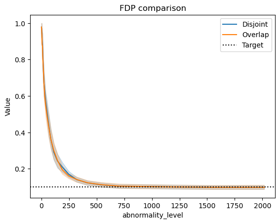
(b) mFDR, $\alpha=0.1$, $\pi=0.02$

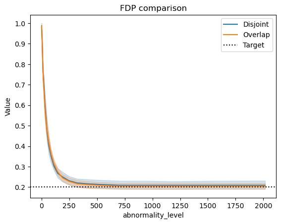
(c) mFDR, $\alpha=0.2$, $\pi=0.02$

(d) FNR, $\alpha=0.1$, $\pi=0.01$

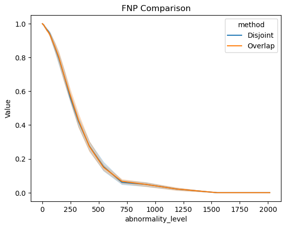
(e) FNR, $\alpha=0.1$, $\pi=0.02$

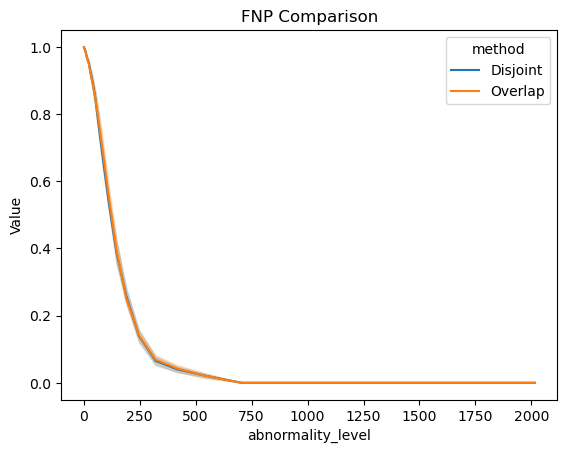
(f) FNR, $\alpha=0.2$, $\pi=0.02$

Figure 14: Effect of atypicity level on mFDR and FNR, depending on whether detection is on disjoint or overlapping subseries

B.4 Figures related to the experiment of Section 5.4

(a) mBH, $4-$sigma

(b) LORD, $4-$sigma

(c) mBH, $3.5-$sigma

(d) LORD, $3.5-$sigma

(e) mBH, $3-$sigma

(f) LORD, $3-$sigma

Figure 15: Comparison of the FDPs acquired from using different multiple testing procedures, mBH or LORD, and from the way the $p$-values are calculated, in the case $\alpha=0.1$.

(a) mBH, $4-$sigma

(b) LORD, $4-$sigma

(a) mBH, $4-$sigma

(b) LORD, $4-$sigma

(c) mBH, $3.5-$sigma

(d) LORD, $3.5-$sigma

(e) mBH, $3-$sigma

(f) LORD, $3-$sigma

Figure 17: Comparison of the FDPs acquired from using different multiple testing procedures, mBH or LORD, and from the way the $p$-values are calculated, in the case $\alpha=0.2$

(a) mBH, $4-$sigma

(b) LORD, $4-$sigma

(c) mBH, $3.5-$sigma

(d) LORD, $3.5-$sigma

(e) mBH, $3-$sigma

(f) LORD, $3-$sigma

Figure 18: Comparison of the FNPs acquired from using different multiple testing procedures, mBH or LORD, and from the way the $p$-values are calculated, in the case $\alpha=0.2$.

References

- [1] {barticle}[author] \bauthor\bsnmAhmed, \bfnmMohiuddin\binitsM., \bauthor\bsnmMahmood, \bfnmAbdun Naser\binitsA. N. and \bauthor\bsnmHu, \bfnmJiankun\binitsJ. (\byear2016). \btitleA survey of network anomaly detection techniques. \bjournalJournal of Network and Computer Applications \bvolume60 \bpages19–31. \endbibitem
- [2] {binproceedings}[author] \bauthor\bsnmAhmed, \bfnmTarem\binitsT. (\byear2009). \btitleOnline anomaly detection using KDE. In \bbooktitleGLOBECOM 2009-2009 IEEE Global Telecommunications Conference \bpages1–8. \bpublisherIEEE. \endbibitem
- [3] {barticle}[author] \bauthor\bsnmAngelopoulos, \bfnmAnastasios N\binitsA. N. and \bauthor\bsnmBates, \bfnmStephen\binitsS. (\byear2021). \btitleA gentle introduction to conformal prediction and distribution-free uncertainty quantification. \bjournalarXiv preprint arXiv:2107.07511. \endbibitem
- [4] {barticle}[author] \bauthor\bsnmBates, \bfnmStephen\binitsS., \bauthor\bsnmCandès, \bfnmEmmanuel\binitsE., \bauthor\bsnmLei, \bfnmLihua\binitsL., \bauthor\bsnmRomano, \bfnmYaniv\binitsY. and \bauthor\bsnmSesia, \bfnmMatteo\binitsM. (\byear2023). \btitleTesting for outliers with conformal p-values. \bjournalThe Annals of Statistics \bvolume51 \bpages149–178. \endbibitem
- [5] {barticle}[author] \bauthor\bsnmBenjamini, \bfnmYoav\binitsY. and \bauthor\bsnmHochberg, \bfnmYosef\binitsY. (\byear1995). \btitleControlling the false discovery rate: a practical and powerful approach to multiple testing. \bjournalJournal of the Royal statistical society: series B (Methodological) \bvolume57 \bpages289–300. \endbibitem
- [6] {barticle}[author] \bauthor\bsnmBenjamini, \bfnmYoav\binitsY. and \bauthor\bsnmYekutieli, \bfnmDaniel\binitsD. (\byear2001). \btitleThe control of the false discovery rate in multiple testing under dependency. \bjournalAnnals of statistics \bpages1165–1188. \endbibitem
- [7] {barticle}[author] \bauthor\bsnmBlázquez-García, \bfnmAne\binitsA., \bauthor\bsnmConde, \bfnmAngel\binitsA., \bauthor\bsnmMori, \bfnmUsue\binitsU. and \bauthor\bsnmLozano, \bfnmJose A\binitsJ. A. (\byear2021). \btitleA review on outlier/anomaly detection in time series data. \bjournalACM Computing Surveys (CSUR) \bvolume54 \bpages1–33. \endbibitem
- [8] {barticle}[author] \bauthor\bsnmBlum, \bfnmJames M\binitsJ. M. and \bauthor\bsnmTremper, \bfnmKevin K\binitsK. K. (\byear2010). \btitleAlarms in the intensive care unit: too much of a good thing is dangerous: is it time to add some intelligence to alarms? \bjournalCritical care medicine \bvolume38 \bpages702–703. \endbibitem
- [9] {binproceedings}[author] \bauthor\bsnmBos, \bfnmHerbert\binitsH. and \bauthor\bsnmHuang, \bfnmKaiming\binitsK. (\byear2006). \btitleTowards software-based signature detection for intrusion prevention on the network card. In \bbooktitleRecent Advances in Intrusion Detection: 8th International Symposium, RAID 2005, Seattle, WA, USA, September 7-9, 2005. Revised Papers 8 \bpages102–123. \bpublisherSpringer. \endbibitem
- [10] {barticle}[author] \bauthor\bsnmBraei, \bfnmMohammad\binitsM. and \bauthor\bsnmWagner, \bfnmSebastian\binitsS. (\byear2020). \btitleAnomaly detection in univariate time-series: A survey on the state-of-the-art. \bjournalarXiv preprint arXiv:2004.00433. \endbibitem
- [11] {binproceedings}[author] \bauthor\bsnmBuda, \bfnmTeodora Sandra\binitsT. S., \bauthor\bsnmCaglayan, \bfnmBora\binitsB. and \bauthor\bsnmAssem, \bfnmHaytham\binitsH. (\byear2018). \btitleDeepad: A generic framework based on deep learning for time series anomaly detection. In \bbooktitlePacific-Asia conference on knowledge discovery and data mining \bpages577–588. \bpublisherSpringer. \endbibitem
- [12] {barticle}[author] \bauthor\bsnmBurnaev, \bfnmEvgeny\binitsE. and \bauthor\bsnmIshimtsev, \bfnmVladislav\binitsV. (\byear2016). \btitleConformalized density-and distance-based anomaly detection in time-series data. \bjournalarXiv preprint arXiv:1608.04585. \endbibitem
- [13] {barticle}[author] \bauthor\bsnmCelisse, \bfnmAlain\binitsA. and \bauthor\bsnmRobin, \bfnmStéphane\binitsS. (\byear2010). \btitleA cross-validation based estimation of the proportion of true null hypotheses. \bjournalJournal of Statistical Planning and Inference \bvolume140 \bpages3132–3147. \endbibitem
- [14] {barticle}[author] \bauthor\bsnmChandola, \bfnmVarun\binitsV., \bauthor\bsnmBanerjee, \bfnmArindam\binitsA. and \bauthor\bsnmKumar, \bfnmVipin\binitsV. (\byear2009). \btitleAnomaly detection: A survey. \bjournalACM computing surveys (CSUR) \bvolume41 \bpages1–58. \endbibitem
- [15] {barticle}[author] \bauthor\bsnmCvach, \bfnmMaria\binitsM. (\byear2012). \btitleMonitor alarm fatigue: an integrative review. \bjournalBiomedical instrumentation & technology \bvolume46 \bpages268–277. \endbibitem
- [16] {barticle}[author] \bauthor\bsnmFisher, \bfnmRA\binitsR. (\byear1951). \btitleThe Design of Experiments, volume 6th Ed. \bjournalHafner, New York, NY. \endbibitem
- [17] {barticle}[author] \bauthor\bsnmFoorthuis, \bfnmRalph\binitsR. (\byear2021). \btitleOn the nature and types of anomalies: a review of deviations in data. \bjournalInternational journal of data science and analytics \bvolume12 \bpages297–331. \endbibitem
- [18] {barticle}[author] \bauthor\bsnmFoster, \bfnmDean P\binitsD. P. and \bauthor\bsnmStine, \bfnmRobert A\binitsR. A. (\byear2008). \btitle-investing: a procedure for sequential control of expected false discoveries. \bjournalJournal of the Royal Statistical Society Series B: Statistical Methodology \bvolume70 \bpages429–444. \endbibitem
- [19] {barticle}[author] \bauthor\bsnmGandy, \bfnmAxel\binitsA. and \bauthor\bsnmHahn, \bfnmGeorg\binitsG. (\byear2014). \btitleMMCTest—a safe algorithm for implementing multiple Monte Carlo tests. \bjournalScandinavian Journal of Statistics \bvolume41 \bpages1083–1101. \endbibitem
- [20] {barticle}[author] \bauthor\bsnmGretton, \bfnmArthur\binitsA., \bauthor\bsnmBorgwardt, \bfnmKarsten M\binitsK. M., \bauthor\bsnmRasch, \bfnmMalte J\binitsM. J., \bauthor\bsnmSchölkopf, \bfnmBernhard\binitsB. and \bauthor\bsnmSmola, \bfnmAlexander\binitsA. (\byear2012). \btitleA kernel two-sample test. \bjournalThe Journal of Machine Learning Research \bvolume13 \bpages723–773. \endbibitem
- [21] {barticle}[author] \bauthor\bsnmGuedj, \bfnmMickael\binitsM., \bauthor\bsnmRobin, \bfnmStephane\binitsS., \bauthor\bsnmCelisse, \bfnmAlain\binitsA. and \bauthor\bsnmNuel, \bfnmGregory\binitsG. (\byear2009). \btitleKerfdr: a semi-parametric kernel-based approach to local false discovery rate estimation. \bjournalBMC bioinformatics \bvolume10 \bpages1–12. \endbibitem
- [22] {barticle}[author] \bauthor\bsnmGuo, \bfnmWenge\binitsW. and \bauthor\bsnmPeddada, \bfnmShyamal\binitsS. (\byear2008). \btitleAdaptive choice of the number of bootstrap samples in large scale multiple testing. \bjournalStatistical applications in genetics and molecular biology \bvolume7. \endbibitem
- [23] {barticle}[author] \bauthor\bsnmHan, \bfnmXingshuo\binitsX., \bauthor\bsnmZhou, \bfnmYuan\binitsY., \bauthor\bsnmChen, \bfnmKangjie\binitsK., \bauthor\bsnmQiu, \bfnmHan\binitsH., \bauthor\bsnmQiu, \bfnmMeikang\binitsM., \bauthor\bsnmLiu, \bfnmYang\binitsY. and \bauthor\bsnmZhang, \bfnmTianwei\binitsT. (\byear2022). \btitleADS-lead: Lifelong anomaly detection in autonomous driving systems. \bjournalIEEE Transactions on Intelligent Transportation Systems \bvolume24 \bpages1039–1051. \endbibitem
- [24] {bbook}[author] \bauthor\bsnmHawkins, \bfnmDouglas M\binitsD. M. (\byear1980). \btitleIdentification of outliers \bvolume11. \bpublisherSpringer. \endbibitem
- [25] {barticle}[author] \bauthor\bsnmHindy, \bfnmHanan\binitsH., \bauthor\bsnmBrosset, \bfnmDavid\binitsD., \bauthor\bsnmBayne, \bfnmEthan\binitsE., \bauthor\bsnmSeeam, \bfnmAmar\binitsA., \bauthor\bsnmTachtatzis, \bfnmChristos\binitsC., \bauthor\bsnmAtkinson, \bfnmRobert\binitsR. and \bauthor\bsnmBellekens, \bfnmXavier\binitsX. (\byear2018). \btitleA taxonomy and survey of intrusion detection system design techniques, network threats and datasets. \endbibitem
- [26] {barticle}[author] \bauthor\bsnmHönes, \bfnmChristoph J\binitsC. J., \bauthor\bsnmMiller, \bfnmBenjamin Kurt\binitsB. K., \bauthor\bsnmHeras, \bfnmAna M\binitsA. M. and \bauthor\bsnmFoing, \bfnmBernard H\binitsB. H. (\byear2021). \btitleAutomatically detecting anomalous exoplanet transits. \bjournalarXiv preprint arXiv:2111.08679. \endbibitem
- [27] {barticle}[author] \bauthor\bsnmHu, \bfnmWeiming\binitsW., \bauthor\bsnmGao, \bfnmJun\binitsJ., \bauthor\bsnmLi, \bfnmBing\binitsB., \bauthor\bsnmWu, \bfnmOu\binitsO., \bauthor\bsnmDu, \bfnmJunping\binitsJ. and \bauthor\bsnmMaybank, \bfnmStephen\binitsS. (\byear2018). \btitleAnomaly detection using local kernel density estimation and context-based regression. \bjournalIEEE Transactions on Knowledge and Data Engineering \bvolume32 \bpages218–233. \endbibitem
- [28] {bincollection}[author] \bauthor\bsnmHuber, \bfnmPeter J\binitsP. J. (\byear1992). \btitleRobust estimation of a location parameter. In \bbooktitleBreakthroughs in statistics: Methodology and distribution \bpages492–518. \bpublisherSpringer. \endbibitem
- [29] {binproceedings}[author] \bauthor\bsnmHundman, \bfnmKyle\binitsK., \bauthor\bsnmConstantinou, \bfnmValentino\binitsV., \bauthor\bsnmLaporte, \bfnmChristopher\binitsC., \bauthor\bsnmColwell, \bfnmIan\binitsI. and \bauthor\bsnmSoderstrom, \bfnmTom\binitsT. (\byear2018). \btitleDetecting spacecraft anomalies using lstms and nonparametric dynamic thresholding. In \bbooktitleProceedings of the 24th ACM SIGKDD international conference on knowledge discovery & data mining \bpages387–395. \endbibitem
- [30] {barticle}[author] \bauthor\bsnmJavanmard, \bfnmAdel\binitsA. and \bauthor\bsnmMontanari, \bfnmAndrea\binitsA. (\byear2018). \btitleOnline rules for control of false discovery rate and false discovery exceedance. \bjournalThe Annals of statistics \bvolume46 \bpages526–554. \endbibitem
- [31] {barticle}[author] \bauthor\bsnmKhraisat, \bfnmAnsam\binitsA., \bauthor\bsnmGondal, \bfnmIqbal\binitsI., \bauthor\bsnmVamplew, \bfnmPeter\binitsP. and \bauthor\bsnmKamruzzaman, \bfnmJoarder\binitsJ. (\byear2019). \btitleSurvey of intrusion detection systems: techniques, datasets and challenges. \bjournalCybersecurity \bvolume2 \bpages1–22. \endbibitem
- [32] {barticle}[author] \bauthor\bsnmKundu, \bfnmArnav\binitsA., \bauthor\bsnmSahu, \bfnmAbhijeet\binitsA., \bauthor\bsnmSerpedin, \bfnmErchin\binitsE. and \bauthor\bsnmDavis, \bfnmKatherine\binitsK. (\byear2020). \btitleA3D: Attention-based auto-encoder anomaly detector for false data injection attacks. \bjournalElectric Power Systems Research \bvolume189 \bpages106795. \endbibitem
- [33] {bphdthesis}[author] \bauthor\bsnmLaxhammar, \bfnmRikard\binitsR. (\byear2014). \btitleConformal anomaly detection: Detecting abnormal trajectories in surveillance applications, \btypePhD thesis, \bpublisherUniversity of Skövde. \endbibitem
- [34] {binproceedings}[author] \bauthor\bsnmLaxhammar, \bfnmRikard\binitsR., \bauthor\bsnmFalkman, \bfnmGoran\binitsG. and \bauthor\bsnmSviestins, \bfnmEgils\binitsE. (\byear2009). \btitleAnomaly detection in sea traffic-a comparison of the gaussian mixture model and the kernel density estimator. In \bbooktitle2009 12th international conference on information fusion \bpages756–763. \bpublisherIEEE. \endbibitem
- [35] {barticle}[author] \bauthor\bsnmLewandowska, \bfnmKatarzyna\binitsK., \bauthor\bsnmMędrzycka-Dąbrowska, \bfnmWioletta\binitsW., \bauthor\bsnmTomaszek, \bfnmLucyna\binitsL. and \bauthor\bsnmWujtewicz, \bfnmMagdalena\binitsM. (\byear2023). \btitleDetermining Factors of Alarm Fatigue among Nurses in Intensive Care Units—A Polish Pilot Study. \bjournalJournal of Clinical Medicine \bvolume12 \bpages3120. \endbibitem
- [36] {binproceedings}[author] \bauthor\bsnmLi, \bfnmDan\binitsD., \bauthor\bsnmChen, \bfnmDacheng\binitsD., \bauthor\bsnmJin, \bfnmBaihong\binitsB., \bauthor\bsnmShi, \bfnmLei\binitsL., \bauthor\bsnmGoh, \bfnmJonathan\binitsJ. and \bauthor\bsnmNg, \bfnmSee-Kiong\binitsS.-K. (\byear2019). \btitleMAD-GAN: Multivariate anomaly detection for time series data with generative adversarial networks. In \bbooktitleInternational conference on artificial neural networks \bpages703–716. \bpublisherSpringer. \endbibitem
- [37] {barticle}[author] \bauthor\bsnmLi, \bfnmHongzu\binitsH. and \bauthor\bsnmBoulanger, \bfnmPierre\binitsP. (\byear2020). \btitleA survey of heart anomaly detection using ambulatory electrocardiogram (ECG). \bjournalSensors \bvolume20 \bpages1461. \endbibitem
- [38] {binproceedings}[author] \bauthor\bsnmLi, \bfnmYang\binitsY., \bauthor\bsnmFang, \bfnmBinxing\binitsB., \bauthor\bsnmGuo, \bfnmLi\binitsL. and \bauthor\bsnmChen, \bfnmYou\binitsY. (\byear2007). \btitleNetwork anomaly detection based on TCM-KNN algorithm. In \bbooktitleProceedings of the 2nd ACM symposium on Information, computer and communications security \bpages13–19. \endbibitem
- [39] {barticle}[author] \bauthor\bsnmLi, \bfnmYichen\binitsY., \bauthor\bsnmZhang, \bfnmXu\binitsX., \bauthor\bsnmHe, \bfnmShilin\binitsS., \bauthor\bsnmChen, \bfnmZhuangbin\binitsZ., \bauthor\bsnmKang, \bfnmYu\binitsY., \bauthor\bsnmLiu, \bfnmJinyang\binitsJ., \bauthor\bsnmLi, \bfnmLiqun\binitsL., \bauthor\bsnmDang, \bfnmYingnong\binitsY., \bauthor\bsnmGao, \bfnmFeng\binitsF., \bauthor\bsnmXu, \bfnmZhangwei\binitsZ. \betalet al. (\byear2022). \btitleAn Intelligent Framework for Timely, Accurate, and Comprehensive Cloud Incident Detection. \bjournalACM SIGOPS Operating Systems Review \bvolume56 \bpages1–7. \endbibitem
- [40] {binproceedings}[author] \bauthor\bsnmMalhotra, \bfnmPankaj\binitsP., \bauthor\bsnmVig, \bfnmLovekesh\binitsL., \bauthor\bsnmShroff, \bfnmGautam\binitsG., \bauthor\bsnmAgarwal, \bfnmPuneet\binitsP. \betalet al. (\byear2015). \btitleLong Short Term Memory Networks for Anomaly Detection in Time Series. In \bbooktitleEsann \bvolume2015 \bpages89. \endbibitem
- [41] {barticle}[author] \bauthor\bsnmMarandon, \bfnmAriane\binitsA., \bauthor\bsnmLei, \bfnmLihua\binitsL., \bauthor\bsnmMary, \bfnmDavid\binitsD. and \bauthor\bsnmRoquain, \bfnmEtienne\binitsE. (\byear2022). \btitleMachine learning meets false discovery rate. \bjournalarXiv preprint arXiv:2208.06685. \endbibitem
- [42] {barticle}[author] \bauthor\bsnmMary, \bfnmDavid\binitsD. and \bauthor\bsnmRoquain, \bfnmEtienne\binitsE. (\byear2022). \btitleSemi-supervised multiple testing. \bjournalElectronic Journal of Statistics \bvolume16 \bpages4926–4981. \endbibitem
- [43] {barticle}[author] \bauthor\bsnmMiele, \bfnmEric Stefan\binitsE. S., \bauthor\bsnmBonacina, \bfnmFabrizio\binitsF. and \bauthor\bsnmCorsini, \bfnmAlessandro\binitsA. (\byear2022). \btitleDeep anomaly detection in horizontal axis wind turbines using graph convolutional autoencoders for multivariate time series. \bjournalEnergy and AI \bvolume8 \bpages100145. \endbibitem
- [44] {barticle}[author] \bauthor\bsnmMunir, \bfnmMohsin\binitsM., \bauthor\bsnmSiddiqui, \bfnmShoaib Ahmed\binitsS. A., \bauthor\bsnmDengel, \bfnmAndreas\binitsA. and \bauthor\bsnmAhmed, \bfnmSheraz\binitsS. (\byear2018). \btitleDeepAnT: A deep learning approach for unsupervised anomaly detection in time series. \bjournalIeee Access \bvolume7 \bpages1991–2005. \endbibitem
- [45] {barticle}[author] \bauthor\bsnmNotaro, \bfnmPaolo\binitsP., \bauthor\bsnmCardoso, \bfnmJorge\binitsJ. and \bauthor\bsnmGerndt, \bfnmMichael\binitsM. (\byear2021). \btitleA survey of aiops methods for failure management. \bjournalACM Transactions on Intelligent Systems and Technology (TIST) \bvolume12 \bpages1–45. \endbibitem
- [46] {binproceedings}[author] \bauthor\bsnmPang, \bfnmGuansong\binitsG., \bauthor\bsnmLi, \bfnmJundong\binitsJ., \bauthor\bparticlevan den \bsnmHengel, \bfnmAnton\binitsA., \bauthor\bsnmCao, \bfnmLongbing\binitsL. and \bauthor\bsnmDietterich, \bfnmThomas G\binitsT. G. (\byear2022). \btitleANDEA: anomaly and novelty detection, explanation, and accommodation. In \bbooktitleProceedings of the 28th ACM SIGKDD Conference on Knowledge Discovery and Data Mining \bpages4892–4893. \endbibitem
- [47] {barticle}[author] \bauthor\bsnmPhipson, \bfnmBelinda\binitsB. and \bauthor\bsnmSmyth, \bfnmGordon K\binitsG. K. (\byear2010). \btitlePermutation P-values should never be zero: calculating exact P-values when permutations are randomly drawn. \bjournalStatistical applications in genetics and molecular biology \bvolume9. \endbibitem
- [48] {barticle}[author] \bauthor\bsnmPincombe, \bfnmBrandon\binitsB. (\byear2005). \btitleAnomaly detection in time series of graphs using arma processes. \bjournalAsor Bulletin \bvolume24 \bpages2. \endbibitem
- [49] {binproceedings}[author] \bauthor\bsnmRamdas, \bfnmAaditya\binitsA., \bauthor\bsnmZrnic, \bfnmTijana\binitsT., \bauthor\bsnmWainwright, \bfnmMartin\binitsM. and \bauthor\bsnmJordan, \bfnmMichael\binitsM. (\byear2018). \btitleSAFFRON: an adaptive algorithm for online control of the false discovery rate. In \bbooktitleInternational conference on machine learning \bpages4286–4294. \bpublisherPMLR. \endbibitem
- [50] {barticle}[author] \bauthor\bsnmRoberts, \bfnmSW\binitsS. (\byear2000). \btitleControl chart tests based on geometric moving averages. \bjournalTechnometrics \bvolume42 \bpages97–101. \endbibitem
- [51] {barticle}[author] \bauthor\bsnmRuff, \bfnmLukas\binitsL., \bauthor\bsnmKauffmann, \bfnmJacob R\binitsJ. R., \bauthor\bsnmVandermeulen, \bfnmRobert A\binitsR. A., \bauthor\bsnmMontavon, \bfnmGrégoire\binitsG., \bauthor\bsnmSamek, \bfnmWojciech\binitsW., \bauthor\bsnmKloft, \bfnmMarius\binitsM., \bauthor\bsnmDietterich, \bfnmThomas G\binitsT. G. and \bauthor\bsnmMüller, \bfnmKlaus-Robert\binitsK.-R. (\byear2021). \btitleA unifying review of deep and shallow anomaly detection. \bjournalProceedings of the IEEE \bvolume109 \bpages756–795. \endbibitem
- [52] {barticle}[author] \bauthor\bsnmSafin, \bfnmAleksandr Maratovich\binitsA. M. and \bauthor\bsnmBurnaev, \bfnmEvgeny\binitsE. (\byear2017). \btitleConformal kernel expected similarity for anomaly detection in time-series data. \bjournalAdvances in Systems Science and Applications \bvolume17 \bpages22–33. \endbibitem
- [53] {binproceedings}[author] \bauthor\bsnmSmith, \bfnmJames\binitsJ., \bauthor\bsnmNouretdinov, \bfnmIlia\binitsI., \bauthor\bsnmCraddock, \bfnmRachel\binitsR., \bauthor\bsnmOffer, \bfnmCharles\binitsC. and \bauthor\bsnmGammerman, \bfnmAlexander\binitsA. (\byear2014). \btitleAnomaly detection of trajectories with kernel density estimation by conformal prediction. In \bbooktitleArtificial Intelligence Applications and Innovations: AIAI 2014 Workshops: CoPA, MHDW, IIVC, and MT4BD, Rhodes, Greece, September 19-21, 2014. Proceedings 10 \bpages271–280. \bpublisherSpringer. \endbibitem
- [54] {barticle}[author] \bauthor\bsnmSolet, \bfnmJo M\binitsJ. M. and \bauthor\bsnmBarach, \bfnmPaul R\binitsP. R. (\byear2012). \btitleManaging alarm fatigue in cardiac care. \bjournalProgress in Pediatric Cardiology \bvolume33 \bpages85–90. \endbibitem
- [55] {binproceedings}[author] \bauthor\bsnmSon, \bfnmSiwoon\binitsS., \bauthor\bsnmGil, \bfnmMyeong-Seon\binitsM.-S. and \bauthor\bsnmMoon, \bfnmYang-Sae\binitsY.-S. (\byear2017). \btitleAnomaly detection for big log data using a Hadoop ecosystem. In \bbooktitle2017 IEEE International Conference on Big Data and Smart Computing (BigComp) \bpages377–380. \bpublisherIEEE. \endbibitem
- [56] {bphdthesis}[author] \bauthor\bsnmStaerman, \bfnmGuillaume\binitsG. (\byear2022). \btitleFunctional anomaly detection and robust estimation, \btypePhD thesis, \bpublisherInstitut polytechnique de Paris. \endbibitem
- [57] {barticle}[author] \bauthor\bsnmStorey, \bfnmJohn D\binitsJ. D., \bauthor\bsnmTaylor, \bfnmJonathan E\binitsJ. E. and \bauthor\bsnmSiegmund, \bfnmDavid\binitsD. (\byear2004). \btitleStrong control, conservative point estimation and simultaneous conservative consistency of false discovery rates: a unified approach. \bjournalJournal of the Royal Statistical Society Series B: Statistical Methodology \bvolume66 \bpages187–205. \endbibitem
- [58] {barticle}[author] \bauthor\bsnmSun, \bfnmWenguang\binitsW. and \bauthor\bsnmCai, \bfnmT Tony\binitsT. T. (\byear2007). \btitleOracle and adaptive compound decision rules for false discovery rate control. \bjournalJournal of the American Statistical Association \bvolume102 \bpages901–912. \endbibitem
- [59] {barticle}[author] \bauthor\bsnmVahdat, \bfnmArash\binitsA. and \bauthor\bsnmKautz, \bfnmJan\binitsJ. (\byear2020). \btitleNVAE: A deep hierarchical variational autoencoder. \bjournalAdvances in neural information processing systems \bvolume33 \bpages19667–19679. \endbibitem
- [60] {binproceedings}[author] \bauthor\bsnmWang, \bfnmWeinan\binitsW., \bauthor\bsnmLiu, \bfnmZhengyi\binitsZ., \bauthor\bsnmShi, \bfnmXiaolin\binitsX. and \bauthor\bsnmPierce, \bfnmLucas\binitsL. (\byear2019). \btitleOnline fdr controlled anomaly detection for streaming time series. In \bbooktitle5th Workshop on Mining and Learning from Time Series (MiLeTS). \endbibitem
- [61] {barticle}[author] \bauthor\bsnmWeinstein, \bfnmAsaf\binitsA., \bauthor\bsnmBarber, \bfnmRina\binitsR. and \bauthor\bsnmCandes, \bfnmEmmanuel\binitsE. (\byear2017). \btitleA power and prediction analysis for knockoffs with lasso statistics. \bjournalarXiv preprint arXiv:1712.06465. \endbibitem
- [62] {binproceedings}[author] \bauthor\bsnmWulsin, \bfnmDrausin\binitsD., \bauthor\bsnmBlanco, \bfnmJustin\binitsJ., \bauthor\bsnmMani, \bfnmRam\binitsR. and \bauthor\bsnmLitt, \bfnmBrian\binitsB. (\byear2010). \btitleSemi-supervised anomaly detection for EEG waveforms using deep belief nets. In \bbooktitle2010 Ninth international conference on machine learning and applications \bpages436–441. \bpublisherIEEE. \endbibitem
- [63] {binproceedings}[author] \bauthor\bsnmXu, \bfnmZiyu\binitsZ. and \bauthor\bsnmRamdas, \bfnmAaditya\binitsA. (\byear2022). \btitleDynamic algorithms for online multiple testing. In \bbooktitleMathematical and Scientific Machine Learning \bpages955–986. \bpublisherPMLR. \endbibitem
- [64] {binproceedings}[author] \bauthor\bsnmZhang, \bfnmMartin\binitsM., \bauthor\bsnmZou, \bfnmJames\binitsJ. and \bauthor\bsnmTse, \bfnmDavid\binitsD. (\byear2019). \btitleAdaptive monte carlo multiple testing via multi-armed bandits. In \bbooktitleInternational Conference on Machine Learning \bpages7512–7522. \bpublisherPMLR. \endbibitem
- [65] {binproceedings}[author] \bauthor\bsnmZhou, \bfnmZeng-Guang\binitsZ.-G. and \bauthor\bsnmTang, \bfnmPing\binitsP. (\byear2016). \btitleContinuous anomaly detection in satellite image time series based on z-scores of season-trend model residuals. In \bbooktitle2016 IEEE International Geoscience and Remote Sensing Symposium (IGARSS) \bpages3410–3413. \bpublisherIEEE. \endbibitem