Convergence Of The Unadjusted Langevin Algorithm For Discontinuous Gradients

Abstract

We demonstrate that for strongly log-convex densities whose potentials are discontinuous on manifolds, the ULA algorithm converges with stepsize bias of order $1/2$ in Wasserstein-p distance. Our resulting bound is then of the same order as the convergence of ULA for gradient Lipschitz potential. Additionally, we show that so long as the gradient of the potential obeys a growth bound (therefore imposing no regularity condition), the algorithm has stepsize bias of order $1/4$. We therefore unite two active areas of research: i) the study of numerical methods for SDEs with discontinuous coefficients and ii) the study of the non-asymptotic bias of the ULA algorithm (and variants). In particular this is the first result of the former kind we are aware of on an unbounded time interval.

1 Introduction

In this paper we consider the overdamped Langevin SDE

$$dY_{t}=-\nabla U(Y_{t})dt+\sqrt{\frac{2}{\beta}}dW_{t},\;\;\;t\geq 0,$$ (1)

where $U:\mathbb{R}^{d}\to\mathbb{R}$ is a potential, $\beta>0$ is the ‘inverse temperature parameter’ and $(W_{t})_{t\geq 0}$ is an $\mathbb{R}^{d}$-valued Wiener martingale independent of the initial condition $\xi$. It is well known that under weak conditions (1) admits the unique invariant measure $\pi_{\beta}\sim e^{-\beta U}$. Given this fact, the overdamped Langevin diffusion has been used as a basis for a variety of sampling and optimization algorithms. In this paper we consider the Unadjusted Langevin Algorithm, or ULA, which is given by the Euler-Maruyama discretisation of (1), or specifically

$$x_{n+1}=x_{n}-\gamma\nabla U(x_{n})+\sqrt{\frac{2\gamma}{\beta}}z_{n+1},\;\;\;x_{0}=\xi,\;\;\;n\in\mathbb{N},$$ (2)

where $\gamma>0$ is the stepize and $(z_{n})_{n\geq 1}$ is a sequence of iid standard Gaussians on $\mathbb{R}^{d}$. This algorithm was first proposed in a physical context in [31] and [13], and in the context of image recognition in [15]. It has been shown to be effective for sampling from Bayesian posteriors, see [30, 34, 10], and utilised as part of a marginal maximal likelihood algorithm in [9]. Theoretical properties of the algorithm have been studied under a Lipschitz assumption on $\nabla U$ and suitable ergodicity properties in [34, 25], and especially thoroughly under the assumption of strong convexity in [10, 5]. A popular variant of the ULA algorithm where the gradient is replaced by an estimate is known as Stochastic Gradient Langevin Dynamics, see [37, 6], and has been analysed under very general conditions in [33, 4, 40]. Furthermore these methods have been extended to constrained problems via the so called ‘projected stochastic gradient Langevin algorithm’, given in [19].

However, even though the ULA algorithm has been adapted to when the gradient is continuous but not globally Lipschitz in [1], we are not aware of any literature on the convergence properties of (2) when $\nabla U$ is not even continuous. The closest thing we are aware of is the strategy of [11, 24, 32], where a discontinuous gradient is smoothed via the computationally-intensive Moreau-Yosida regularisation. Additionally, the case of SGLD with discontinuous stochastic gradient was considered in [22, 23, 35], however with the assumption of a ‘continuity in average’ condition which excludes truly discontinuous densities.

On the other hand, in the context of numerical methods for SDEs (on bounded time intervals), there has been a flurry of research in recent years addressing this issue, see [36] for a survey. Two main lines of research have appeared: Strategy I, for which $L^{p}$ convergence rate of $1/2$ has been proven for SDEs with piecewise-Lipschitz drift and multiplicative noise in [29], and Strategy II, for which an $L^{2}$ convergence rate of $1/2-$ has been proven for SDEs with additive noise and drift that is merely bounded and measurable in [7]. The technique of Strategy I involves a judicious choice of ‘transformation function’ which smooths the discontinuity of the drift, in addition to bounds on the intervals in which the scheme crosses a point of discontinuity. It has been expanded to the case where the drift is superlinear in [27], to the multidimensional case (where the discontinuities lie on manifolds) in [21], and to a convergence rate $3/4$ when the drift is piecewise smooth in [28]. The technique of Strategy II involve involve the regularising properties of the noise, and been extended to the case of Levy processes in [3], multiplicative noise in [8] and SPDEs in [2]. These generalisations in particular make use the stochastic sewing lemma established in [20]. We note that whilst Strategy II is more general, it has not yet been adapted to the case where the coefficients of the SDE are unbounded. Lower bounds which demonstrate the optimality of many of results from Strategy I and II results have been established in [17, 26].

Therefore, in the present work we unite these two lines of research and prove in Theorem 1 that the ULA algorithm (2) converges with $L^{p}$ discretisation error of order $1/2$ (uniformly in time). We assume that $U$ is strongly convex, and Lipschitz outside of a collection of sufficiently smooth compact hypersurfaces. Whilst we use techniques inspired in part by the strategy of [29], due to monotonicity of $\nabla U$ we shall not need to use a transformation function, which means the collection of hypersurfaces considered can intersect in an arbitrary manner. The main technical challenge then is to extend the work discussed in the previous paragraph to an unbounded time interval. To do this we shall multiply the difference process between the scheme and the true solution by an appropriate exponential and apply Proposition 3, which demonstrates that the scheme does not cross the hypersurfaces of discontinuity too often (weighted by an exponential function of time). A key ingredient in the proof of Proposition 3 is the occupation time formula Lemma 7, which is a corollary of the classical local time identity.

One disadvantage of Theorem 1 is that it requires A 1, which states that the discontinuities lie on a compact manifold. This therefore rules out many relevant examples where the discontinuity lies on an unbounded manifold, say a hyperplane. This is the case for instance for the examples considered in [11]. However, using a much simpler argument than in Theorem 1, we show in Theorem 2 that no matter how irregular $\nabla U$ is, so long as it obeys a linear growth bound the numerical error of the Euler scheme in $L^{p}$ is of order $1/4$ uniformly in time. This therefore demonstrates that the Euler scheme is broadly ‘robust’ in the case where $\nabla U$ is convex, in the sense that the discretisation error does indeed converge to $0$ at polynomial rate as the stepsize tends to $0$. This is in contrast to the general case for the Euler scheme, where even for bounded coefficients the scheme can converge to the true solution arbitrarily slowly, see [16, 38].

1.1 Assumptions

We assume strong convexity of $U$ (which implies strong monotonicity of $\nabla U$) in A 2 below, as well as the integrability of the initial condition $\xi$. For the regularity of $\nabla U$ we have two different assumptions. For Theorem 1 we have A 1, in which we assume there are open sets $\Phi_{j}\subset\mathbb{R}^{d}$ (the union of whose completion is $\mathbb{R}^{d}$) on which $\nabla U$ is (piecewise) Lipschitz continuous, and that the boundary of these open sets is a subset of a collection of sufficiently regular compact hypersurfaces. We do not require that $\nabla U$ be well defined on the boundary of the $\Phi_{j}$, and indeed $\nabla U$ will never be well defined at a point of discontinuity. In Proposition 1 we prove that all processes of interest are well defined none the less. Note that unlike in [21], one does not require that the union of the hypersurfaces $\Sigma_{i}$ be smooth overall.

As an alternative to A 1 we have the much weaker assumption B 1 for Theorem 2, which places no requirement on the regularity of $\nabla U$ at all besides that it is well-defined almost everywhere and does not grow superlinearly. This weaker assumption comes at the cost of a weaker numerical error of order $1/4$.

Note that in A 3 we assume $\xi$ is such that $\nabla U(\xi)$ is almost surely well defined (so that in particular $\xi$ takes values in $\cup^{n_{2}}_{j=1}\Sigma_{j}$ with probability $0$). This is necessary since otherwise the first iteration of (2) will not be well defined. This however causes us no problems beyond the initial condition, as we show in Proposition 1.

A 1.

(Piecewise Continuity) There exist bounded regions $M_{j}\subset\mathbb{R}^{d}$ and compact, orientable, connected, $C^{3}$ hypersurfaces $\Sigma_{j}\subset\mathbb{R}^{d}$ such that $\Sigma_{j}=\partial M_{j}$ for $j=1,2,...,n_{2}$. Furthermore these hypersurfaces cut $\mathbb{R}^{d}$ into smaller regions, that is, there exist disjoint open sets $\Phi_{i}\subset\mathbb{R}^{d}$, $i=1,2,...,n_{1}$ such that $\cup_{i=1}^{n_{1}}\overline{\Phi}_{i}=\mathbb{R}^{d}$ and $\cup_{i=1}^{m}\partial\Phi_{i}\subset\cup_{j=1}^{n_{2}}\Sigma_{j}$. Then $\nabla U$ is piecewise-Lipschitz on the $\Phi_{i}$. Specifically, there exists $L>0$ such that

$$\lvert\nabla U(x)-\nabla U(y)\rvert\leq L\lvert x-y\rvert,\;\;\;x,y\in\Phi_{i},\;\;\;i=1,2,...,n_{1}.$$ (3)

B 1.

(Growth Assumption) The function $\nabla U:\mathbb{R}^{d}\to\mathbb{R}^{d}$ exists almost everywhere, and there exists $L,m>0$ such that

$$\lvert\nabla U(x)\rvert\leq m+L\lvert x\rvert.$$ (4)

A 2.

(Strong Monotonicity) There exists $\mu>0$ such that

$$\langle\nabla U(x)-\nabla U(y),x-y\rangle\geq\mu\lvert x-y\rvert^{2},\;\;\;x,y\in\mathbb{R}^{d}.$$ (5)

A 3.

(Integrable Initial Condition) One has $P(\xi\in\{x\in\mathbb{R}^{d}|\;\nabla U(x)\;\text{well defined}\})=1$. Additionally, for every $p>0$ one has

$$E\lvert\xi\rvert^{p}<\infty$$ (6)

Since each of the $\Sigma_{j}$ are compact, there exists an $R>0$ large enough that $\cup^{n_{2}}_{i=1}\Sigma^{\delta}_{i}\subset B_{R}$. Therefore only one of the $\Phi_{i}$ is unbounded, and we can assume without loss of generality that it is $\Phi_{1}$ is unbounded.

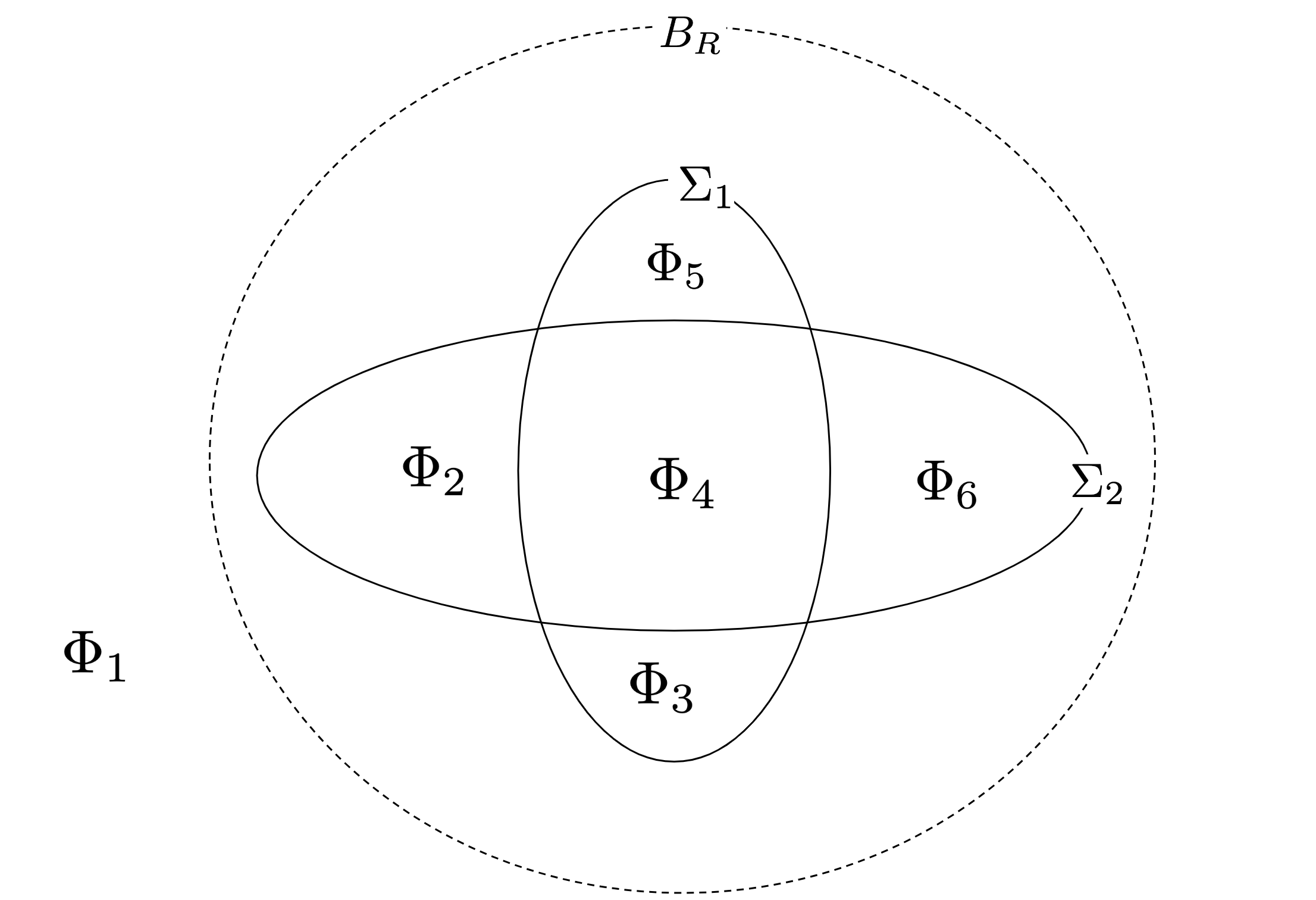
Figure 1: Under A 1 we have that the hypersurfaces $\Sigma_{j}$ cut $\mathbb{R}^{d}$ into regions $\Phi_{i}$ on which $\nabla U$ is continuous. Additionally, $R>0$ is large enough that $\cup^{n_{2}}_{i=1}\Sigma^{\delta}_{i}\subset B_{R}$, and of the $\Phi_{i}$ only $\Phi_{1}$ is unbounded. Note that in this diagram $M_{j}$, $j=1,2$ are the interiors of the two hypersurfaces, so that $M_{1}=\Phi_{3}\cup\Phi_{4}\cup\Phi_{5}$ and $M_{2}=\Phi_{2}\cup\Phi_{4}\cup\Phi_{6}$.

1.2 Well-Posedness and Set-Up

In this section we show that the problem is well-posed despite the fact $\nabla U$ is only defined almost everywhere (and in particular, is not in general defined on the $\Sigma_{i}$). Firstly let us first define the continuous interpolation of (2). Let $\kappa_{\gamma}(t):=\gamma\lfloor\frac{t}{\gamma}\rfloor$ be the backwards projection onto the grid $\{0,\gamma,2\gamma,...\}$, so that $\kappa_{\gamma}(n\gamma+\epsilon)=n\gamma$ for $n\in\mathbb{N}$ and $\epsilon\in[0,\gamma)$. Furthermore let $\underline{\kappa}_{\gamma}(t):=\kappa_{\gamma}(t)+\gamma$ be the forward projection onto $\{0,\gamma,2\gamma,...\}$. Then one may define

$$X_{t}=\xi-\int^{t}_{0}\nabla U(X_{\kappa_{\gamma}(s)})ds+\sqrt{\frac{2}{\beta}}W_{t}.$$ (7)

Setting $z_{n}:=\frac{W_{n\gamma}-W_{(n-1)\gamma}}{\sqrt{\gamma}}$ one then sees by this definition that $X_{n\gamma}=x_{n}$ for all $n\in\mathbb{N}$. From now on it will mostly be more convenient to analyse (7).

Proposition 1.

Let B 1 and A 3 hold. Then for every non-random initial condition $\xi=x\in\mathbb{R}^{d}\setminus\cup^{n_{2}}_{j=1}\Sigma_{j}$ the SDEs (1) and (7) have well-defined unique strong solutions.

Proof.

The unique strong solution of (1) follows from Theorem 2.1 in [39]. For (7) to be well defined, by the structure of the Euler scheme we just have to show that $P(X_{n\gamma}\in\{x\in\mathbb{R}^{d}|\;\nabla U(x)\;\text{well defined}\})=1$ for every $n\in\mathbb{N}$ and initial condition $x\in\mathbb{R}^{d}\setminus\cup^{n_{2}}_{j=1}\Sigma_{j}$. Note that $\mathcal{L}(X_{n\gamma})=\mathcal{L}(x_{n})$, so it sufficient to check $P(x_{n}\in\cup_{i=1}^{n_{1}}\Sigma_{i})=0$ for every $n\geq 0$. Since $x_{0}=\xi$ this holds by A 3 for $n=0$. Then it holds for $n\geq 1$ since the law of $x_{n}$ conditioned on $x_{n-1}\in\mathbb{R}^{d}\setminus\cup^{n_{2}}_{j=1}\Sigma_{j}$ is absolutely continuous with respect to the Lesbesgue measure for every $n\geq 1$. ∎

Since (1) and (7) have strong solutions for every non-random initial condition $\xi=x\in\mathbb{R}^{d}\setminus\cup^{n_{2}}_{j=1}\Sigma_{j}$, one may set up the probability space for $(Y_{t})_{t\geq 0}$ and $(X_{t})_{t\geq 0}$ as follows. Let $(\Omega_{1},\mathcal{H}^{1},P_{1})$ be a probability space on which $\xi$ is defined and let $(\Omega_{2},(\mathcal{H}^{2}_{t})_{t\geq 0},P_{2})$ be a filtered probability space on which $(W_{t})_{t\geq 0}$ is defined and adapted to. Then one can define the probability space $(\Omega,(\mathcal{F}_{t})_{t\geq 0},P)$ as the product of the two probability spaces, so that $\Omega=\Omega_{1}\times\Omega_{2}$, $dP(\omega)=dP(\omega_{1},\omega_{2})=dP_{1}(\omega_{1})dP_{2}(\omega_{2})$ and $\mathcal{F}_{t}=\mathcal{H}^{2}_{t}\times\mathcal{H}^{1}$. Then for $x\in\mathbb{R}^{d}\setminus\cup^{n_{2}}_{j=1}\Sigma_{j}$, the map $\omega=(\omega_{1},\omega_{2})\mapsto X^{x}_{t}(\omega_{2})$ can be defined as the strong solution to

$$X^{x}_{t}=x-\int^{t}_{0}\nabla U(X^{x}_{\kappa_{\gamma}(s)})ds+\sqrt{\frac{2}{\beta}}W_{t},$$ (8)

and under A 3, one has $X_{t}(\omega)=X_{t}(\omega_{1},\omega_{2}):=X^{\xi(\omega_{1})}_{t}(\omega_{2})$. Then for all measurable functionals $f$ from measurable functions into $\mathbb{R}$, one may define

$$E^{x}f((X_{t})_{t\geq 0}):=Ef((X^{x}_{t})_{t\geq 0}),$$ (9)

and additionally for all Borel-measurable subsets $A$ of functions $\mathbb{R}^{d}\to\mathbb{R}$, one may define $P^{x}((X_{t})_{t\geq 0}\in A):=P((X^{x}_{t})_{t\geq 0}\in A)$. One can similarly define the process $(Y^{x}_{t})_{t\geq 0}$ and extend these definitions to (1). Therefore $E^{x}$ corresponds to the conditional definition $E^{x}[\cdot]=E[\cdot|\;\xi=x]$. Furthermore by Fubini’s Theorem, given the integrand is uniformly integrable and $P(\xi\in\mathbb{R}^{d}\setminus\cup^{n_{2}}_{j=1}\Sigma_{j})=0$ one has

$$E[\cdot]=\int_{\mathbb{R}^{d}\setminus\cup^{n_{2}}_{j=1}\Sigma_{j}}E^{x}[\cdot]d\mu_{\xi}(x),$$ (10)

where $\mu_{\xi}$ is the law of $\xi$. It follows that if, for any random variable $z$, we may define the random operator $E^{z}[\cdot]$ by

$$\omega\mapsto E^{z(\omega)}[\cdot].$$ (11)

Then one has

Lemma 1.

Consider the definition (11). Then for every $n\in\mathbb{N}$, $t\geq 0$ and measurable function $f:\mathbb{R}^{d}\to\mathbb{R}$ one has

$$E^{X^{x}_{n\gamma}}[f(X_{t})]=E^{x}[f(X_{t+n\gamma})|\mathcal{F}_{n\gamma}],\;\;\;E^{X_{n\gamma}}[f(X_{t})]=E[f(X_{t+n\gamma})|\mathcal{F}_{n\gamma}].$$ (12)

Proof.

Due to the discrete Euler Scheme structure of $X_{t}$, for every $x\in\mathbb{R}^{d}$ and $t\geq 0$ there exists $m\in\mathbb{N}$ and a function $u^{x}_{t}:(\mathbb{R}^{d})^{m}\to\mathbb{R}^{d}$ such that

$$u^{x}_{t}(W_{\gamma},W_{2\gamma}-W_{\gamma},...,W_{\kappa_{\gamma}(t)}-W_{\kappa_{\gamma}(t)-\gamma},W_{t}-W_{\kappa_{\gamma}(t)})=X^{x}_{t},$$ (13)

almost surely (where the last argument is obviously supressed if $t=\kappa_{\gamma}(t)$). Therefore

$$E^{x}[f(X_{t+n\gamma})|\mathcal{F}_{n\gamma}] =E[f(u^{x}_{t+n\gamma}(W_{\gamma},W_{2\gamma}-W_{\gamma},...,W_{t+n\gamma}-W_{\kappa_{\gamma}(t)+n\gamma}))|\mathcal{F}_{n\gamma}]$$

$$=\int_{\Omega}f(u^{x}_{t+n\gamma}(W_{\gamma},W_{2\gamma}-W_{\gamma},...,W_{n\gamma}-W_{(n-1)\gamma},z))d\mu(z),$$ (14)

where we have compressed all arguments of $u^{x}_{t+n\gamma}$ after the $n$th into $z$, and denoted the respective law $\mu$. The fact that we can take expectation of over all random inputs independent of $\mathcal{F}_{n\gamma}$ follows in the same way as Example 4.1.7 from [12]. Furthermore observe that by the Markov property of $X_{0},X_{\gamma},X_{2\gamma}$ one has

$$u^{x}_{t+n\gamma}(w_{1},...,w_{n+m})=u_{t}^{u^{x}_{n\gamma}(w_{1},...,w_{n})}(w_{n+1},...,w_{n+m}),$$ (15)

so that

$$E^{x}[f(X_{t+n\gamma})|\mathcal{F}_{n\gamma}](\omega)=\int_{\Omega}f(u^{X^{x}_{n\gamma}(\omega)}_{t}(z))d\mu(z)=E^{X^{x}_{n\gamma}(\omega)}[f(X_{t})].$$ (16)

The first result then follows. For the second, one integrates $x$ with respect to the law of $\xi$, the initial condition of $X_{t}$. ∎

1.3 Delta-Neighbourhood

Essential for the following arguments shall be the constant $\delta>0$ given below, which provides a good neighbourhood of the $\Sigma_{i}$ on which to perform our analysis. Let us first define for $j=1,2,...,n_{2}$ the signed distance function

$$\rho_{j}(x)=\begin{cases}dist(x,\Sigma_{j}),\;\;\;\;\;x\in\mathbb{R}^{d}\setminus M_{j}\\ 0,\;\;\;\;\;\;\;\;x\in\Sigma_{j}\\ -dist(x,\Sigma_{i}),\;\;\;x\in M_{j},\end{cases}$$ (17)

and, for $\epsilon>0$, the epsilon neighbourhood

$$\Sigma^{\epsilon}:=\{x\in\mathbb{R}^{d}\;|\;dist(x,\Sigma)<\epsilon\}.$$ (18)

Proposition 2.

There exists a constant $\delta>0$ such that for every $j=1,2,...,n_{2}$

1. one has that $\rho_{j}\in C^{2}(\Sigma_{j}^{3\delta})$

2. for every $x\in\Sigma_{j}^{3\delta}$, one has $\lvert\nabla\rho_{j}(x)\rvert=1$

Proof.

The first part follows from the statement of [14], Lemma 14.16, choosing $\delta=\mu/3$ for $\mu$ as in the Lemma. The second part follows from the last two lines of the proof, where it is shown that for every $x\in\Sigma_{j}^{3\delta}$ there exists $y\in\Sigma_{j}$ such that $\nabla\rho_{j}(x)=n_{j}(y)$, where $n_{j}$ is the unit normal to $\Sigma_{j}$. Therefore $\lvert\nabla\rho_{j}(x)\rvert=\lvert n_{j}(y)\rvert=1$. ∎

It follows that if we define $\phi\in C^{\infty}(\mathbb{R})$ to be a smooth cutoff function satisfying $\phi=1$ on $[-\delta,\delta]$ and $\phi=0$ outside of $(-2\delta,2\delta)$, one has that $P_{j}:=\phi\circ\rho_{j}$ satisfies $P_{j}=\rho_{j}$ on $\Sigma_{j}^{\delta}$ and $P_{j}\in C^{2}(\mathbb{R}^{d})$. This will be useful in order to apply Ito’s formula in the proof of Lemma 6.

1.4 Main Theorems

Now we present our main results: note that replacing the piecewise Lipschitz assumption A 1 with the weaker growth assumption B 1 leads to a weakening of the order of numerical error from $1/2$ to $1/4$.

Theorem 1.

Let A 1, A 2 and A 3 hold. Let $p\geq 1$ and $\beta>0$. Consider $\pi_{\beta}\sim e^{-\beta U}$, the invariant measure of the overdamped Langevin diffusion (1). Let $\gamma_{0}\in(0,\frac{\mu}{2L^{2}})$. Then there exists $c>0$ such that for every $\gamma\in(0,\gamma_{0})$ the unadjusted Langevin algorithm (ULA) given in (2) satisfies

$$W_{p}(\pi_{\beta},\mathcal{L}(x_{n}))\leq W_{p}(\xi,\pi_{\beta})e^{-\mu\gamma n}+c\gamma^{1/2}.$$ (19)

Theorem 2.

Let B 1, A 2 and A 3 hold. Let $p\geq 1$, $\beta>0$, $\pi_{\beta}$ and $\gamma_{0}>0$ be as above. Then there exists $c>0$ such that for every $\gamma\in(0,\gamma_{0})$ the unadjusted Langevin algorithm (ULA) given in (2) satisfies

$$W_{p}(\pi_{\beta},\mathcal{L}(x_{n}))\leq W_{p}(\xi,\pi_{\beta})e^{-\mu\gamma n}+c\gamma^{1/4}.$$ (20)

Remark 1.

We note that Theorem 1 replicates the numerical error of order $1/2$, established in the case where $\nabla U$ is Lipschitz in [10] (see Proposition 3 and Corollary 7). A numerical error of order $1$ is also established in the same paper under the assumption $\nabla U$ is smooth (see Corollary 9). However, it is shown in [28] that in general the Euler scheme cannot converge faster than rate $3/4$ for discontinuous drifts, which suggests that Theorem 1 cannot be improved beyond numerical error of order $3/4$.

Remark 2.

For the Lipschitz case, letting $L>0$ denote the Lipschitz constant, the stepsize restriction is $\gamma\leq\frac{1}{\mu+L}$ (see [10]). This is comparable to our stepsize restriction in the case $\mu\sim L$, as in the case for instance where $\nabla U(x)$ is a perturbation of $\mu x$, so that $\pi_{\beta}$ is a perturbation of a Gaussian. However as $L\to\infty$ for fixed $\mu$, the stepsize restriction in Theorems 1 and 2 scales like $O(L^{-2})$ compare to $O(L^{-1})$ in [10].

Remark 3.

Since the arguments in Section 3 are significantly intricate, we choose not to track any dependence besides the step-size $\gamma>0$. However, one can nonetheless make the important observation that the bound in Theorem 1 blows up as $\beta\to\infty$. This arises due to (58) and (3), which cause the bound in Lemma 7 to scale with $\beta$, and therefore (due to (3)) causes the bound in Lemma 8 to scale similarly. Therefore, our results can be seen as an example of ‘regularisation by noise’, since the noise is essential for avoiding pathological behaviour, and our arguments become less effective as the process becomes more deterministic. This is in contrast to Theorem 2, where the bound will strengthen as $\beta\to\infty$, since the error in Theorem 2 depends on the increment bound in Lemma 4, which will decrease and in fact be of order $O(l^{p})$ in the $\beta\to\infty$ limit.

Although we have presented Theorems 1 and 2 in terms of Wasserstein distance (as is standard in the algorithms literature), we prove the theorem by obtaining bounds in $L^{p}$ of the kind common in the numerics literature, see (101). In particular, we show that that if $Y_{0}=X_{0}=\xi$, then under the hypothesis of Theorem 1 one has

$$\sup_{t\geq 0}\;(E[\lvert Y_{t}-X_{t}\rvert^{p}])^{1/p}\leq c\gamma^{1/2},$$ (21)

and similarly under the hypothesis of Theorem 2 one has

$$\sup_{t\geq 0}\;(E[\lvert Y_{t}-X_{t}\rvert^{p}])^{1/p}\leq c\gamma^{1/4}.$$ (22)

2 Preliminary Bounds

Note 1.

From now on the generic constant $c>0$ changes from line to line and is independent of the stepsize $\gamma>0$ and time parameters $t,s,u>0$.

Note 2.

We use often the following corollary of Young’s inequality: for every $p,q>0$ and $a>0$ there exists $c>0$ such that $x^{p}y^{q}\leq ax^{p+q}+cy^{p+q}$. This follows by applying Young’s inequality to $x^{p}y^{q}=(a^{\frac{p}{p+q}}x^{p})(a^{-\frac{p}{p+q}}y^{q})$.

In this section we prove standard moment and increment bounds for the Langevin dynamics (1), the Euler scheme (2) and and its continuous interpolation (7). These bounds are very similar to those in [10] and other references, with minor alterations to account for the lack of continuity of $\nabla U$. Recall that A 1 implies B 1.

All Lemmas in Sections 2 and 3 are proven under the expectation $E^{x}$ defined in Section 1.2 (which implies the same bound under $E$ with the use of A 3). This is due to the proof of Proposition 3, where the dependence on the initial condition (and the fact that the $\Sigma_{j}$ lie in a compact set) is used at the conclusion of the proof.

Lemma 2.

Let B 1 and A 2 hold. Let $p>0$ and $x\in\mathbb{R}^{d}\setminus\cup_{j=1}^{n_{2}}\Sigma_{j}$. Then one has

$$\sup_{t\geq 0}E^{x}\lvert Y_{t}\rvert^{p}\leq c(1+\lvert x\rvert^{p}).$$ (23)

Proof.

Let $\tau_{R}:=\inf\{t\geq 0|\;\lvert Y_{t}\rvert=R\}$. Then one may begin by applying Itô’s formula on $[0,\tau_{R}\wedge t]$, so that by the boundedness of the coefficients under B 1, the stochastic integral vanishes and one obtains

$$E^{x}e^{p\mu(\tau_{R}\wedge t)/4}\lvert Y_{\tau_{R}\wedge t}\rvert^{p} =\lvert x\rvert^{p}+E^{x}\int^{\tau_{R}\wedge t}_{0}e^{p\mu s/4}(\frac{p\mu}{4}\lvert Y_{s}\rvert^{p}-p\langle\nabla U(Y_{s}),Y_{s}\rangle\lvert Y_{s}\rvert^{p-2}+c\lvert Y_{s}\rvert^{p-2})ds,$$ (24)

Now let us assume without loss of generality that $\nabla U(0)$ is well defined (since $\nabla U$ is well defined almost everywhere, this holds up to a slight shift of the coordinate system). Then we may use A 2 to write

$$-\langle\nabla U(x),x\rangle \leq-\langle\nabla U(x)-\nabla U(0),x\rangle-\langle\nabla U(0),x\rangle$$

$$\leq-\mu\lvert x\rvert^{2}+\frac{\mu}{2}\lvert x\rvert^{2}+\frac{2}{\mu}\lvert\nabla U(0)\rvert^{2}$$

$$\leq-\frac{\mu}{2}\lvert x\rvert^{2}+c,$$ (25)

so that applying this bound, and using Young’s inequality to bound the last term (see Note 2) as

$$c\lvert Y_{s}\rvert^{p-2}\leq\frac{p\mu}{4}\lvert Y_{s}\rvert^{p}+c,$$ (26)

one has

$$E^{x}e^{p\mu(\tau_{R}\wedge t)/4}\lvert Y_{\tau_{R}\wedge t}\rvert^{p} =\lvert x\rvert^{p}+c\int^{\tau_{R}\wedge t}_{0}e^{p\mu s/4}ds\leq\lvert x\rvert^{p}+ce^{p\mu(\tau_{R}\wedge t)/4}\leq\lvert x\rvert^{p}+ce^{p\mu t/4}.$$ (27)

Now observe that by continuity $\sup_{s\in[0,t]}\lvert Y_{s}\rvert<\infty$ almost surely, so that by Fatou’s Lemma

$$\liminf_{R\to\infty}E^{x}e^{p\mu(\tau_{R}\wedge t)/4}\lvert Y_{\tau_{R}\wedge t}\rvert^{p}\geq E^{x}\liminf_{R\to\infty}e^{p\mu(\tau_{R}\wedge t)/4}\lvert Y_{\tau_{R}\wedge t}\rvert^{p}=e^{p\mu t/4}E^{x}\lvert Y_{t}\rvert^{p}.$$ (28)

Therefore since the RHS of (27) is independent of $R$, we may take $\liminf_{R\to\infty}$ and divide through by $e^{p\mu t/4}$, so that

$$E^{x}\lvert Y_{t}\rvert^{p}\leq e^{-p\mu t/4}\lvert x\rvert^{p}+c\leq\lvert x\rvert^{p}+c,$$ (29)

at which point the result follows since this bound is independent of $t\geq 0$. ∎

Lemma 3.

Let B 1 and A 2 hold. Let $p>0$. Let $\gamma_{0}\in(0,\frac{\mu}{2L^{2}})$. Then there exists $c>0$ such that for every $\gamma\in(0,\gamma_{0})$ and $x\in\mathbb{R}^{d}\setminus\cup_{j=1}^{n_{2}}\Sigma_{j}$ one has

$$\sup_{t\geq 0}E^{x}\lvert X_{t}\rvert^{p}\leq c(1+\lvert x\rvert^{p}).$$ (30)

Proof.

Let us fix $\gamma_{0}\in(0,\frac{\mu}{2L^{2}})$ and consider $X_{t}$ for stepsize $\gamma\in(0,\gamma_{0})$. Recalling the discrete definition in (2), we begin by proving

$$\sup_{n\geq 0}E^{x}\lvert x_{n}\rvert^{2}\leq c(1+\lvert x\rvert^{2}).$$ (31)

Let us begin by applying B 1 and (2) and calculating

$$\lvert x_{n}-\gamma\nabla U(x_{n})\rvert^{2} =\lvert x_{n}\rvert^{2}+\gamma^{2}\lvert\nabla U(x_{n})\rvert^{2}-2\gamma\langle\nabla U(x_{n}),x_{n}\rangle$$

$$\leq r(\gamma)\lvert x_{n}\rvert^{2}+c\gamma,$$

where $r(\gamma):=\max\{1-\gamma\mu+2L^{2}\gamma^{2},0\}$, since if $1-\gamma\mu+2L^{2}\gamma^{2}\leq 0$, we may bound by $0$. Then one has by the definition of (2) that

$$\lvert x_{n+1}\rvert^{2}\leq r(\gamma)\lvert x_{n}\rvert^{2}+c\gamma+\frac{2\gamma}{\beta}\lvert z_{n+1}\rvert^{2}+2\langle x_{n}-\gamma\nabla U(x_{n}),\sqrt{\frac{2\gamma}{\beta}}z_{n+1}\rangle$$ (32)

so that denoting $\eta_{i+1}:=2\sqrt{\gamma}\langle x_{n}-\gamma\nabla U(x_{n}),\sqrt{\frac{2}{\beta}}z_{i+1}\rangle$ one may use the standard identity that, for sequences $a_{n},b_{n}\in\mathbb{R}$ and $r>0$ satisfying $a_{n+1}\leq ra_{n}+b_{n}$, one has

$$a_{n}\leq r^{n}a_{0}+\sum_{i=0}^{n-1}r^{i}b_{i},$$ (33)

to calculate that

$$\lvert x_{n}\rvert^{2}\leq r(\gamma)^{n}\lvert x_{0}\rvert^{2}+c\gamma\sum^{n-1}_{i=0}r(\gamma)^{i}+\sum^{n-1}_{i=0}(\frac{2\gamma}{\beta}\lvert z_{i+1}\rvert^{2}+\eta_{i+1})r(\gamma)^{i}.$$ (34)

Then since $x_{n}$ is independent of $z_{n+1}$, one has $E^{x}\eta_{i}=0$ for every $i\geq 1$. As a result, one has that

$$E^{x}\lvert x_{n}\rvert^{2}\leq\lvert x\rvert^{2}+c\frac{1}{1-r(\gamma)}\leq\lvert x\rvert^{2}+c\frac{1}{2\mu-4L^{2}\gamma}.$$ (35)

Note that since $\gamma_{0}\in(0,\frac{\mu}{2L^{2}})$, these bounds are uniform over $\gamma\in(0,\gamma_{0})$ and $n\in\mathbb{N}$, so (31) follows. Now let us assume

$$\sup_{n\geq 0}E^{x}\lvert x_{n}\rvert^{p}\leq c(1+\lvert x\rvert^{p}),$$ (36)

holds for $p=2q$ for $q\in\mathbb{N}$. Let us prove by induction it therefore holds for $p=2q+2$, thus proving (36) for $p\in 2\mathbb{N}$, at which point the result follows for all $p>0$, by Jensen’s inequality. To this end let us raise (32) to the power of $q+1$, expand into polynomial factors and take expectation, so that by B 1 and the inductive moments bound assumption

$$E^{x}\lvert x_{n+1}\rvert^{2q+2}\leq r(\gamma)^{q+1}E^{x}\lvert x_{n}\rvert^{2q+2}+c\gamma,$$ (37)

since all terms of lower order in $\gamma$ vanish due to the independence of $z_{n+1}$ with $x_{n}$. Therefore

$$E^{x}\lvert x_{n+1}\rvert^{2q+2}\leq r(\gamma)^{n(q+1)}\lvert x\rvert^{2q+2}+c\gamma\frac{1}{1-r(\gamma)^{q+1}},$$ (38)

and so since $r(\gamma)^{q/2+1}\leq r(\gamma)<1$ one has

$$E^{x}\lvert x_{n+1}\rvert^{2q+2}\leq r(\gamma)^{n(q+1)}\lvert x\rvert^{2q+2}+c\gamma\frac{1}{1-r(\gamma)}\leq\lvert x\rvert^{2q+2}+\frac{1}{2\mu-4L^{2}\gamma},$$ (39)

and (36) follows uniformly over $\gamma\in(0,\gamma_{0})$ for $p=2q+2$, as required. Now for the full result observe that by Hölder’s inequality

$$\lvert X_{t}\rvert^{p} =c\lvert X_{t}-X_{\kappa_{\gamma}(t)}\rvert^{p}+c\lvert X_{\kappa_{\gamma}(t)}\rvert^{p}$$

$$\leq c\gamma^{p-1}\int^{t}_{\kappa_{\gamma}(t)}\lvert\nabla U(X_{\kappa_{\gamma}(t)})\rvert^{p}ds+c\lvert W_{t}-W_{\kappa_{\gamma}(t)}\rvert^{p}+c\lvert X_{\kappa_{\gamma}(t)}\rvert^{p},$$ (40)

at which point one applies B 1 to obtain

$$\lvert X_{t}\rvert^{p}\leq c\lvert X_{\kappa_{\gamma}(t)}\rvert^{p}+c\lvert W_{t}-W_{\kappa_{\gamma}(t)}\rvert^{p},$$ (41)

and the result follows by applying expectation, since $X_{\kappa_{\gamma}(t)}=x_{\kappa_{\gamma}(t)/\gamma}$. ∎

Lemma 4.

Let B 1 and A 2 hold. Let $p,s>0$ and $l\in[0,1]$. Let $\gamma_{0}\in(0,\frac{\mu}{2L^{2}})$. Then there exists $c>0$ such that for every $\gamma\in(0,\gamma_{0})$ and $x\in\mathbb{R}^{d}\setminus\cup_{j=1}^{n_{2}}\Sigma_{j}$

$$E^{x}\sup_{u\in[s,s+l]}\lvert X_{u}-X_{s}\rvert^{p}\leq cl^{p/2}(1+\lvert x\rvert^{p}).$$ (42)

Proof.

One has

$$\lvert X_{u}-X_{s}\rvert\leq\int^{u}_{s}\lvert\nabla U(X_{\kappa_{\gamma}(s)})\rvert ds+\sqrt{\frac{2\gamma}{\beta}}\lvert W_{u}-W_{s}\rvert,$$ (43)

so that taking supremum and raising to the power $p$, by Hölder’s inequality one has

$$\sup_{u\in[s,s+l]}\lvert X_{u}-X_{s}\rvert^{p}\leq cl^{p-1}\int^{s+l}_{s}\lvert\nabla U(X_{\kappa_{\gamma}(s)})\rvert^{p}ds+c\biggr{(}\frac{2\gamma}{\beta}\biggr{)}^{p/2}\sup_{u\in[s,s+l]}\lvert W_{u}-W_{s}\rvert^{p},$$ (44)

and therefore taking expectation and applying B 1 and Lemma 3, the result follows. ∎

Lemma 5.

Let B 1 and A 2 hold. Let (1) have starting condition $Y_{0}=\xi$. Then

$$W_{p}(\pi_{\beta},\mathcal{L}(Y_{t}))\leq W_{p}(\xi,\pi_{\beta})e^{-\mu\gamma n}.$$ (45)

Proof.

Let $(\tilde{Y}_{t})_{t\geq 0}$ be a solution of (1), driven by the same noise as $(Y_{t})_{t\geq 0}$ but with initial condition $\tilde{Y}_{0}=\tilde{\xi}$ satisfying $\mathcal{L}(\tilde{\xi})=\pi_{\beta}$. Then since $\pi_{\beta}$ is the invariant measure of (1), for all $t\geq 0$ one has $\mathcal{L}(\tilde{Y}_{t})=\pi_{\beta}$. One then calculates by the chain rule (since $Y_{t}-\tilde{Y_{t}}$ has vanishing diffusion) that

$$e^{p\mu t}E\lvert Y_{t}-\tilde{Y_{t}}\rvert^{p} =E\lvert\xi-\tilde{\xi}\rvert^{p}+\int^{t}_{0}p\mu e^{p\mu s}\lvert Y_{s}-\tilde{Y_{s}}\rvert^{p}ds$$

$$+p\int^{t}_{0}e^{p\mu s}\langle Y_{s}-\tilde{Y_{s}},\nabla U(Y_{s})-\nabla U(\tilde{Y_{s}})\rangle\lvert Y_{s}-\tilde{Y_{s}}\rvert^{p-2}ds,$$ (46)

so that applying the convexity assumption A 2 and dividing through by $e^{p\mu t}$

$$E\lvert Y_{t}-\tilde{Y_{t}}\rvert^{p}\leq e^{-p\mu t}E\lvert\xi-\tilde{\xi}\rvert^{p}.$$ (47)

Then the result follows since one has the trivial bound $W_{p}(\pi_{\beta},\mathcal{L}(Y_{t}))^{p}\leq E\lvert Y_{t}-\tilde{Y_{t}}\rvert^{p}$, and by optimising the coupling of $\xi$ and $\tilde{\xi}$ by the definition of the Wasserstein distance. ∎

3 Crossing Bounds

Since $\nabla U$ is not continuous, under A 1 we can only bound the crucial discretisation term $\lvert\nabla U(X_{u})-\nabla U(X_{\kappa_{\gamma}(u)})\rvert$ when $X_{u}$ and $X_{\kappa_{\gamma}(u)}$ both lie in the same $\Phi_{i}$ for some $i=1,2,...,n_{1}$. In this section we prove that this is the case a large amount of the time on an unbounded interval. In particular, in Proposition 3 we show that the $p$th moment of the $du$-measure of the time $X_{u}$ and $X_{\kappa_{\gamma}(u)}$ spend in different of the $\Phi_{i}$ on $[0,t]$, weighted by $e^{qu}$, is $O(\gamma^{p/2}e^{pqt})$. The exponential weighting here follows from the proof of Theorem 1, where one scales the discretisation error by an appropriate exponential in order to prove bounds that are uniform in time.

The strategy of this section is as follows. In Lemmas 6 and 7 we show how you can use the classical local time identity to yield a local time identity for functions of the process integrated on $[t,t+1]$ for $t\geq 0$. In Lemma 8 we use this to bound the times in which $X_{u}$ and $X_{\kappa_{\gamma}(u)}$ lie in different $\Phi_{i}$, for $u\in[t,t+1]$. In Lemma 9 we extend the previous lemma to the unbounded interval $[0,t]$, weighted by an exponential. Finally in Proposition 3 we prove the full result.

Lemma 6.

Let A 1 and A 2 hold. Let $\gamma_{0}\in(0,\frac{\mu}{2L^{2}})$. Let $P_{j}$ be the local signed distance function to $\Sigma_{j}$ given in Section 1.3 for $j=1,2,...,n_{2}$. Let $\mathcal{L}^{a,j}_{t}$ denote the local time of $P_{j}(X)$ at $a\in\mathbb{R}$ and time $t\geq 0$. Then there exists $c>0$ such that for every $t\geq 0$, $\gamma\in(0,\gamma_{0})$, $a\in[-\delta,\delta]$, $j\in\{1,2,...,n_{2}\}$ and $x\in\mathbb{R}^{d}\setminus\cup_{j=1}^{n_{2}}\Sigma_{j}$ one has

$$E^{x}\mathcal{L}^{a,j}_{t}\leq c(1+\lvert x\rvert)(1+t),$$ (48)

$$E^{x}(\mathcal{L}^{a,j}_{t+1}-\mathcal{L}^{a,j}_{t})\leq c(1+\lvert x\rvert).$$ (49)

Proof.

Since $P_{j}\in C^{2}(\mathbb{R}^{d})$ one may apply the classical Itô’s formula to obtain

$$P_{j}(X_{t})=P_{j}(\xi)+\int^{t}_{0}\biggr{(}-\nabla P_{j}(X_{u})\nabla U(X_{\kappa_{\gamma}(u)})+\frac{1}{\beta}\Delta P_{j}(X_{\kappa_{\gamma}(u)})\biggr{)}du+\sqrt{\frac{2}{\beta}}\int^{t}_{0}\nabla P_{j}(X_{u})dW_{u}$$ (50)

Therefore by the classical local time identity, or Tanaka-Meyer identity (see (7.9) on page 220 in [18]), one has

$$E^{x}\mathcal{L}^{a,j}_{t} =\frac{1}{2}E^{x}\lvert P_{j}(X_{t})-a\rvert-\frac{1}{2}\lvert P_{j}(x)-a\rvert-\frac{1}{2}E^{x}\int^{t}_{0}sign(P_{j}(X_{s})-a)\nabla P_{j}(X_{s})\nabla U(X_{\kappa_{\gamma}(s)})ds$$

$$-\frac{1}{2\beta}E^{x}\int^{t}_{0}sign(P_{j}(X_{s})-a)\Delta P_{j}(X_{s})ds,$$ (51)

Now observe that since $P_{j}\in C^{2}(\mathbb{R}^{d})$ and is supported on a compact set, $P_{j}$, $\nabla P_{j}$ and $\nabla^{2}P_{j}$ are bounded. Therefore

$$E^{x}\mathcal{L}^{a,j}_{t} \leq\frac{1}{2}E^{x}\lvert P_{j}(X_{t})-a\rvert-\frac{1}{2}\lvert P_{j}(x)-a\rvert+c\int^{t}_{0}E^{x}\lvert\nabla U(X_{\kappa_{\gamma}(s)})\rvert ds$$

$$-\frac{1}{2\beta}E^{x}\int^{t}_{0}sign(P_{j}(X_{s})-a)\Delta P_{j}(X_{s})ds,$$ (52)

so by the triangle inequality, B 1 (since A 1 implies B 1) and Lemma 3, one can ensure all terms are above bounded by $c(1+\lvert x\rvert)(1+t)$, and (48) follows. For the second bound first observe that by the triangle inequality

$$\lvert P_{j}(X_{t+1})-a\rvert-\lvert P_{j}(X_{t})-a\rvert\leq\lvert P_{j}(X_{t+1})-P_{j}(X_{t})\rvert,$$ (53)

so that by (3) one has that the difference $E^{x}\mathcal{L}^{a,j}_{t+1}-E^{x}\mathcal{L}^{a,j}_{t}$ is given by integrals over $[t,t+1]$ and (53), so one may obtain

$$E^{x}\mathcal{L}^{a,j}_{t+1}-E^{x}\mathcal{L}^{a,j}_{t} \leq E^{x}\lvert P_{j}(X_{t+1})-P_{j}(X_{t})\rvert+c.$$ (54)

Now observe that additionally $P_{j}$ is Lipschitz since it has uniformly bounded first derivative, at which point (49) follows from Lemma 4 with $l=1$. ∎

Lemma 7.

Let A 1 and A 2 hold. Let $\gamma_{0}\in(0,\frac{\mu}{2L^{2}})$. Let $g:\mathbb{R}\to\mathbb{R}$ satisfy $0\leq g\leq c$ and suppose $supp(g)\subset(-\delta,\delta)$ for $\delta>0$ as in Proposition 2. Then there exists $c>0$ such that for every $t\geq 0$, $\gamma\in(0,\gamma_{0})$, $a\in[-\delta,\delta]$, $j\in\{1,2,...,n_{2}\}$ and $x\in\mathbb{R}^{d}\setminus\cup_{j=1}^{n_{2}}\Sigma_{j}$ one has

$$E^{x}\int^{t+1}_{t}g(P_{j}(X_{s}))ds\leq c(1+\lvert x\rvert)\int^{\delta}_{-\delta}g(s)ds.$$ (55)

Proof.

Let us denote the quadratic variation of $P_{j}(X)$ by $\langle P_{j}(X)\rangle_{s}$. Then since $supp(g)\subset(-\delta,\delta)$, and $P_{j}(x)\in[-\delta,\delta]$ implies $x\in\Sigma_{j}^{\delta}$, one has

$$\int^{t}_{0}g(P_{j}(X_{s}))d\langle P_{j}(X)\rangle_{s}=\frac{2}{\beta}\int^{t}_{0}g(P_{j}(X_{s}))\lvert\nabla P_{j}(X_{s})\rvert^{2}ds=\frac{2}{\beta}\int^{t}_{0}g(P_{j}(X_{s}))\lvert\nabla P_{j}(X_{s})\rvert^{2}1_{X_{s}\in\Sigma_{j}^{\delta}}ds,$$ (56)

so that since $\lvert\nabla\rho_{j}(x)\rvert=\lvert\nabla P_{j}(x)\rvert=1$ for every $x\in\Sigma_{j}^{\delta}$ by Proposition 2, one has

$$\int^{t}_{0}g(P_{j}(X_{s}))ds=\frac{\beta}{2}\int^{t}_{0}g(P_{j}(X_{s}))d\langle P_{j}(X)\rangle_{s}.$$ (57)

Therefore, by the classical local time identity, i.e. Theorem 7.1 iii) page 218 in [18], one obtains

$$E^{x}\int^{t}_{0}g(P_{j}(X_{s}))ds=\frac{\beta}{2}\int^{t}_{0}E^{x}g(P_{j}(X_{s}))d\langle P_{j}(X)\rangle_{s}=\frac{\beta}{2}\int^{\delta}_{-\delta}g(a)E^{x}\mathcal{L}^{a,j}_{t}da,$$ (58)

so that

$$E^{x}\int^{t+1}_{t}g(P_{i}(X_{s}))ds =E^{x}\int^{t+1}_{0}g(P_{i}(X_{s}))ds-E^{x}\int^{t}_{0}g(P_{i}(X_{s}))ds$$

$$=\frac{\beta}{2}\int^{\delta}_{-\delta}g(a)E^{x}(\mathcal{L}^{a,j}_{t+1}-\mathcal{L}^{a,j}_{t})da,$$ (59)

and therefore the result follows from Lemma 6. ∎

Lemma 8.

Let A 1 and A 2 hold. Let $\gamma_{0}\in(0,\frac{\mu}{2L^{2}})$. Then there exists $c>0$ such that for every $t\geq 0$, $\gamma\in(0,\gamma_{0})$ and $x\in\mathbb{R}^{d}\setminus\cup_{j=1}^{n_{2}}\Sigma_{j}$ one has

$$E^{x}\int^{t+1}_{t}1_{A_{u}}du\leq c(1+\lvert x\rvert^{3})\gamma^{1/2},$$

where

$$A_{s}:=\{\text{There does not exist}\;i\in\{1,2,...,m\}\;\text{such that}\;X_{s},X_{\kappa_{\gamma}(s)}\in\Phi_{i}\}.$$ (60)

Proof.

Step i) Let us fix a time $t\geq 0$ and $j\in\{1,2,...,n_{2}\}$. Then we may define a stopped version of $X_{s}$ which is equal to $X_{s}$ unless there happens to be a $u\in[t,t+1]$ for which $\lvert X_{u}-X_{\kappa_{\gamma}(u)}\rvert\geq 1$, at the first instance of which it stops. Specifically

$$\tau:=\inf\{u\in[t,t+1+\gamma]\;|\;\lvert X_{u}-X_{\kappa_{\gamma}(u)}\rvert\geq 1\}\cup\{\infty\},\;\;\;\bar{X}_{s}:=X_{s\wedge\tau},\;\;\;s\geq 0.$$ (61)

Let us define the stopped version of $K^{j}_{s}$ from the next step as

$$\bar{K}^{j}_{s}:=\biggr{\{}\sup_{u\in[s,s+\gamma]}\lvert\bar{X}_{u}-\bar{X}_{s}\rvert\geq dist(\bar{X}_{s},\Sigma_{j})\biggr{\}},\;\;\;s\geq 0,$$ (62)

and (recalling $\tau\geq t$ by definition) let us prove

$$E^{x}\int^{(t+1)\wedge\tau}_{t}1_{\bar{K}^{j}_{s}}ds\leq c(1+\lvert x\rvert)\gamma^{1/2}.$$ (63)

To this end we may split as

$$\int^{(t+1)\wedge\tau}_{t}1_{\bar{K}^{j}_{s}}ds =\int^{(t+1)\wedge\tau}_{t}1_{\bar{K}^{j}_{s}}\cdot 1_{\bar{X}_{s}\in\Sigma_{j}^{\delta}}ds+\int^{(t+1)\wedge\tau}_{t}1_{\bar{K}^{j}_{s}}\cdot 1_{\bar{X}_{s}\not\in\Sigma_{j}^{\delta}}ds$$

$$=:v_{1}+v_{2}.$$ (64)

Now let us show that there exists $c_{1}>0$ such that for every $\omega\in\{\bar{X}_{s}\in\Sigma_{j}^{\delta}\}$ and $s\in[t,t+1]$ one has

$$\sup_{u\in[s,s+\gamma]}\lvert\bar{X}_{s}(\omega)-\bar{X}_{u}(\omega)\rvert\leq c_{1}\biggr{(}\gamma+\sup_{u\in[s,s+\gamma]}\lvert W_{s}(\omega)-W_{u}(\omega)\rvert\biggr{)}.$$ (65)

Let $s\in[t,t+1]$ and $l\in[s,s+\gamma]$. Then

$$\lvert\bar{X}_{s}-\bar{X}_{l}\rvert \leq\biggr{\lvert}\int^{l\wedge\tau}_{s\wedge\tau}\nabla U(\bar{X}_{\kappa_{\gamma}(v)})dv+\sqrt{\frac{2}{\beta}}(W_{s\wedge\tau}-W_{l\wedge\tau})\biggr{\rvert}$$

$$\leq\int^{s+\gamma}_{s}\lvert\nabla U(\bar{X}_{\kappa_{\gamma}(v)})\rvert dv+\sqrt{\frac{2}{\beta}}\sup_{u\in[s,s+\gamma]}\lvert W_{s}-W_{u}\rvert,$$ (66)

so that since the bound is independent of $l$ one has

$$\sup_{u\in[s,s+\gamma]}\lvert\bar{X}_{s}-\bar{X}_{u}\rvert\leq\int^{s+\gamma}_{s}\lvert\nabla U(\bar{X}_{\kappa_{\gamma}(v)})\rvert dv+\sqrt{\frac{2}{\beta}}\sup_{u\in[s,s+\gamma]}\lvert W_{s}-W_{u}\rvert.$$ (67)

Now note for $v\in[s,s+\gamma]$ one has $\kappa_{\gamma}(v)\in\{\kappa_{\gamma}(s),\underline{\kappa}_{\gamma}(s)\}$, where $\underline{\kappa}_{\gamma}$ is the forward projection onto the discretisation grid given in Section 1.2. Let us show we can bound the integrand above uniformly for $\omega\in\{\bar{X}_{s}\in\Sigma_{j}^{\delta}\}$.

Figure 2: Recall that the coefficients of (7) change at $\kappa_{\gamma}(s)$ and $\underline{\kappa}_{\gamma}(s)$

First note that since $\Sigma_{j}^{\delta}\subset B_{R}$ for $R>0$ as in Section 1.1, one has that $\omega\in\{\bar{X}_{s}\in\Sigma_{j}^{\delta}\}$ implies that $\lvert\bar{X}_{s}(\omega)\rvert\leq R$. Therefore, by the definition of the stopped process in (61), for such an $\omega\in\{\bar{X}_{s}\in\Sigma_{j}^{\delta}\}$ one has

$$\lvert\bar{X}_{\kappa_{\gamma}(s)}(\omega)\rvert\leq\lvert\bar{X}_{s}(\omega)\rvert+\lvert\bar{X}_{s}(\omega)-\bar{X}_{\kappa_{\gamma}(s)}(\omega)\rvert\leq R+1,$$ (68)

and

$$\lvert\bar{X}_{\underline{\kappa}_{\gamma}(s)}(\omega)\rvert \leq\lvert\bar{X}_{s}(\omega)\rvert+\lvert\bar{X}_{s}(\omega)-\bar{X}_{\underline{\kappa}_{\gamma}(s)}(\omega)\rvert$$

$$\leq\lvert\bar{X}_{s}(\omega)\rvert+\lvert\bar{X}_{s}(\omega)-\bar{X}_{\kappa_{\gamma}(s)}(\omega)\rvert+\lvert\bar{X}_{\kappa_{\gamma}(s)}(\omega)-\bar{X}_{\underline{\kappa}_{\gamma}(s)}(\omega)\rvert\leq R+2,$$ (69)

where the third term in the final line is bounded by $1$ by continuity, and since for $s\in[t,t+1]$ one has $\underline{\kappa}_{\gamma}(s)\leq t+1+\gamma$. Then since $\nabla U$ is bounded on compact sets, one has for $\omega\in\{\bar{X}_{s}\in\Sigma_{j}^{\delta}\}$ that

$$\int^{s+\gamma}_{s}\lvert\nabla U(\bar{X}_{\kappa_{\gamma}(v)}(\omega))\rvert dv\leq c\gamma,$$ (70)

at which point (65) follows. Now let us denote (for all $\omega\in\Omega$)

$$h_{s}:=c_{1}\biggr{(}\gamma+\sup_{u\in[s,s+\gamma]}\lvert W_{u}-W_{s}\rvert\biggr{)}.$$ (71)

so that we have, by the definition of $\rho_{j}$ given in Section 1.3

$$1_{K^{j}_{s}}\cdot 1_{\bar{X}_{s}\in\Sigma_{j}^{\delta}}\leq 1_{\{h_{s}\geq dist(\bar{X}_{s},\Sigma_{j}^{\delta})\}}\cdot 1_{\bar{X}_{s}\in\Sigma_{j}^{\delta}}=1_{\{h_{s}\geq\lvert\rho_{j}(\bar{X}_{s})\rvert\}}\cdot 1_{\bar{X}_{s}\in\Sigma_{j}^{\delta}}.$$ (72)

As a result, since $\bar{X}_{s}=X_{s}$ for $s\in[0,\tau]$, one may write

$$v_{1} =\int^{(t+1)\wedge\tau}_{t}1_{\bar{K}^{j}_{s}}\cdot 1_{\bar{X}_{s}\in\Sigma_{j}^{\delta}}ds\leq\int^{(t+1)\wedge\tau}_{t}1_{\{h_{s}\geq\lvert\rho_{j}(\bar{X}_{s})\rvert\}}\cdot 1_{\bar{X}_{s}\in\Sigma_{j}^{\delta}}ds$$

$$=\int^{(t+1)\wedge\tau}_{t}1_{\{h_{s}\geq\lvert\rho_{j}(X_{s})\rvert\}}\cdot 1_{X_{s}\in\Sigma_{j}^{\delta}}ds\leq\int^{t+1}_{t}1_{\{h_{s}\geq\lvert\rho_{j}(X_{s})\rvert\}}\cdot 1_{X_{s}\in\Sigma_{j}^{\delta}}ds.$$ (73)

Now recall that for independent random variables $X$ and $Y$ one has that

$$E[f(X,Y)|X]=g(X),$$ (74)

where $g(x):=Ef(x,Y)$. Therefore, since $h_{s}$ is independent of $X_{s}$, one may write

$$E^{x}[1_{\{h_{s}\geq\lvert\rho_{i}(X_{s})\rvert\}}\cdot 1_{X_{s}\in\Sigma_{j}^{\delta}}]=E^{x}\biggr{[}E^{x}[1_{\{h_{s}\geq\lvert\rho_{i}(X_{s})\rvert\}}\cdot 1_{X_{s}\in\Sigma_{j}^{\delta}}\;|\;X_{s}]\biggr{]}$$

$$=E^{x}\biggr{[}E^{x}[1_{\{h_{s}\geq\lvert\rho_{i}(X_{s})\rvert\}}\cdot 1_{\lvert\rho_{i}(X_{s})\rvert\leq\delta}\;|\;\rho_{i}(X_{s})]\biggr{]}=E^{x}[g(\rho_{i}(X_{s}))],$$ (75)

where since $\mathcal{L}(h_{s})=\mathcal{L}(h_{0})$ for $s\geq 0$, one may define $g:\mathbb{R}\to\mathbb{R}$ as

$$g(x)=P(\lvert x\rvert\leq h_{0})1_{\lvert x\rvert\leq\delta}.$$ (76)

Therefore, by the definition of $h_{s}$ in (71), one has $Eh_{0}=\leq c\gamma^{1/2}$, and by Lemma 7 one has

$$E^{x}v_{1} \leq E^{x}\int^{t+1}_{t}g(\rho_{i}(X_{s}))ds\leq c(1+\lvert x\rvert)\int^{\delta}_{-\delta}g(s)ds\leq c(1+\lvert x\rvert)\int^{\delta}_{0}P(s\leq h_{0})ds$$

$$\leq c(1+\lvert x\rvert)\int^{\infty}_{0}P(s\leq h_{0})ds\leq c(1+\lvert x\rvert)Eh_{0}\leq c(1+\lvert x\rvert)\gamma^{1/2}.$$ (77)

Now for $v_{2}$ we observe that

$$K^{j}_{s}\cap\{\bar{X}_{s}\not\in\Sigma_{j}^{\delta}\}\subset\{\sup_{u\in[s,s+\gamma]}\lvert\bar{X}_{u}-\bar{X}_{s}\rvert\geq\delta\},$$ (78)

so by Markov’s inequality and Lemma 4

$$E^{x}v_{2}\leq\int^{t+1}_{t}P^{x}(\sup_{u\in[s,s+\gamma]}\lvert\bar{X}_{u}-\bar{X}_{s}\rvert\geq\delta)ds\leq c(1+\lvert x\rvert)\gamma^{1/2},$$ (79)

at which point substituting (3) and (79) into (3), the result in (63) follows.

Step ii) Now we prove the unstopped version of (63), that is for $t\geq 0$, $j\in\{1,2,...,n_{2}\}$ and $K^{j}_{s}$ given as

$$K^{j}_{s}:=\biggr{\{}\sup_{u\in[s,s+\gamma]}\lvert X_{u}-X_{s}\rvert\geq dist(X_{s},\Sigma_{j})\biggr{\}}.$$ (80)

we prove

$$E^{x}\int^{t+1}_{t}1_{K^{j}_{u}}du\leq c(1+\lvert x\rvert)\gamma^{1/2}.$$ (81)

In the case where $\tau=\infty$, one has

$$1_{\tau=\infty}\cdot\int^{t+1}_{t}1_{K^{j}_{s}}ds\leq\int^{(t+1)\wedge\tau}_{t}1_{\bar{K}^{j}_{s}}ds,$$ (82)

so one may use (63) to bound as

$$E^{x}\biggr{[}1_{\tau=\infty}\cdot\int^{t+1}_{t}1_{K^{j}_{s}}ds\biggr{]}\leq c(1+\lvert x\rvert)\gamma^{1/2}.$$ (83)

For the case where $\tau\in[t,t+1]$, one may bound $1_{K^{j}_{u}}\leq 1$ so that

$$E^{x}\biggr{[}1_{\tau\in[t,t+1]}\cdot\int^{t+1}_{t}1_{K^{j}_{u}}du\biggr{]}\leq P^{x}(\tau\in[t,t+1]).$$ (84)

Now observing that $\tau\in[t,t+1]$ implies that there exists a $u\in[t,t+1]$ such that $\lvert X_{u}-X_{\kappa_{\gamma}(u)}\rvert\geq 1$, one has

$$\{\tau\in[t,t+1]\}\subset\{\sup_{u\in[t,\underline{\kappa}_{\gamma}(t)]}\lvert X_{t}-X_{u}\rvert\geq 1\}\cup\biggr{(}\bigcup_{i=0}^{\lfloor 1/\gamma\rfloor}\{\sup_{u\in[\underline{\kappa}_{\gamma}(t)+i\gamma,\underline{\kappa}_{\gamma}(t)+(i+1)\gamma]}\lvert X_{i\gamma}-X_{u}\rvert\geq 1\}\biggr{)},$$

one may write

$$P^{x}(\tau\in[t,t+1]) \leq P^{x}(\sup_{u\in[t,\underline{\kappa}_{\gamma}(t)]}\lvert X_{t}-X_{u}\rvert\geq 1)+\sum^{\lfloor 1/\gamma\rfloor}_{i=0}P^{x}\biggr{(}\sup_{u\in[\underline{\kappa}_{\gamma}(t)+i\gamma,\underline{\kappa}_{\gamma}(t)+(i+1)\gamma]}\lvert X_{i\gamma}-X_{u}\rvert\geq 1\biggr{)}$$

$$=P^{x}(\sup_{u\in[t,\underline{\kappa}_{\gamma}(t)]}\lvert X_{t}-X_{u}\rvert^{3}\geq 1)+\sum^{\lfloor 1/\gamma\rfloor}_{i=0}P^{x}\biggr{(}\sup_{u\in[\underline{\kappa}_{\gamma}(t)+i\gamma,\underline{\kappa}_{\gamma}(t)+(i+1)\gamma]}\lvert X_{i\gamma}-X_{u}\rvert^{3}\geq 1\biggr{)}.$$

Then applying Markov’s inequality and Lemma 4, one obtains that

$$P^{x}(\tau\in[t,t+1])\leq c(\lfloor 1/\gamma\rfloor+1)(1+\lvert x\rvert^{3})\gamma^{3/2}\leq c(1+\lvert x\rvert^{3})\gamma^{1/2},$$ (85)

which one may substitute into (84) to obtain

$$E^{x}\biggr{[}1_{\tau\in[t,t+1]}\cdot\int^{t+1}_{t}1_{K^{j}_{s}}ds\biggr{]}\leq c(1+\lvert x\rvert^{3})\gamma^{1/2},$$ (86)

so that summing (83) and (86), one has that (81) follows.

Step iii) Now we prove the result for $A_{s}$. Suppose $\omega\in(\cup_{j=1}^{n_{2}}K^{j}_{s-\gamma})^{c}$ for $s\geq\gamma$. Then $\sup_{u\in[s-\gamma,s]}\lvert X_{u}-X_{s}\rvert<dist(X_{s},\Sigma_{j})$ for every $j=1,,2,...,n_{2}$, so since $\cup_{i=1}^{n_{1}}\partial\Phi_{i}\subset\cup_{j=1}^{n_{2}}\Sigma_{j}$, the process can’t have reached the boundary of any $\Phi_{j}$. Therefore it has stayed in the same $\Phi_{i}$, or in other words there must exist a $i^{\prime}$ such that $X_{u}\in\Phi_{i^{\prime}}$ for every $u\in[s-\gamma,s]$. Therefore $\omega\in(A_{s})^{c}$ also. Negating this relation one obtains

$$A_{s}\subset\cup_{j=1}^{n_{2}}K^{j}_{s-\gamma}.$$ (87)

Now let us assumme $\gamma\leq 1$ (if not the result follows trivially). Then we may bound $1_{A_{u}}$ by $1$ on $[t,t+\gamma]$ to obtain

$$E^{x}\int^{t+1}_{t}1_{A_{u}}du=\gamma+E^{x}\int^{t+1}_{t+\gamma}1_{A_{u}}du\leq\gamma+\sum_{j=1}^{n_{2}}E^{x}\int^{t+1}_{t}1_{K^{j}_{u}}du\leq c(1+\lvert x\rvert^{3})\gamma^{1/2}$$ (88)

by (81). ∎

Lemma 9.

Let A 1 and A 2 hold. Let $\gamma_{0}\in(0,\frac{\mu}{2L^{2}})$. Then there exists $c>0$ such that for every $t\geq 0$, $\gamma\in(0,\gamma_{0})$ and $x\in\mathbb{R}^{d}\setminus\cup_{j=1}^{n_{2}}\Sigma_{j}$ one has

$$E^{x}\int^{t}_{0}e^{qs}1_{A_{s}}ds\leq c(1+\lvert x\rvert^{3})\gamma^{1/2}e^{qt},$$

where $A_{s}$ is given in Lemma 8.

Proof.

Let us split $[0,t]$ into unit intervals up to $\lfloor t\rfloor$, and bound the exponential by its supremum on each interval. Then one obtains

$$\int^{t}_{0}e^{qs}1_{A_{s}}ds=\sum_{i=1}^{\lfloor t\rfloor}\int^{i}_{i-1}e^{qs}1_{A_{s}}ds+\int^{t}_{\lfloor t\rfloor}e^{qs}1_{A_{s}}ds\leq\sum_{i=1}^{\lfloor t\rfloor}e^{qi}\int^{i}_{i-1}1_{A_{s}}ds+e^{qt}\int^{t}_{\lfloor t\rfloor}1_{A_{s}}ds.$$ (89)

Then by Lemma 8 one has

$$E^{x}\int^{t}_{0}e^{qu}1_{A_{u}}du \leq\sum_{i=1}^{\lfloor t\rfloor}e^{qi}E^{x}\int^{i}_{i-1}1_{A_{s}}ds+e^{qt}E^{x}\int^{\lfloor t\rfloor+1}_{\lfloor t\rfloor}1_{A_{s}}ds$$

$$\leq c(1+\lvert x\rvert^{3})\gamma^{1/2}\biggr{(}\sum_{i=1}^{\lfloor t\rfloor}e^{qi}+e^{qt}\biggr{)}.$$

Now observe that since $e^{qi}\leq e^{qu}$ for $u\in[i,i+1]$, one has

$$\sum_{i=1}^{\lfloor t\rfloor}e^{qi}\leq\sum_{i=1}^{\lfloor t\rfloor-1}\int^{i+1}_{i}e^{qu}du+e^{q\lfloor t\rfloor}\leq\int^{\lfloor t\rfloor}_{1}e^{qu}du+e^{q\lfloor t\rfloor}\leq ce^{qt},$$ (90)

at which point the result follows. ∎

Proposition 3.

Let A 1 and A 2 hold. Let $\gamma_{0}\in(0,\frac{\mu}{2L^{2}})$ and $p\geq 0$. Then there exists $c>0$ such that for every $t\geq 0$, $\gamma\in(0,\gamma_{0})$ and $x\in\mathbb{R}^{d}\setminus\cup_{j=1}^{n_{2}}\Sigma_{j}$ one has

$$E\biggr{[}\int^{t}_{0}e^{qs}1_{A_{s}}ds\biggr{]}^{p}\leq c\gamma^{p/2}e^{pqt},$$

where $A_{s}$ is given in Lemma 8.

Proof.

We prove for $p\in\mathbb{N}$, at which point all other values of $p>0$ follow by Jensen’s inequality and taking appropriate roots. Furthermore, we prove by induction, where the base case follows from Lemma 8, the initial condition identity (10) and the integrability of the initial condition in Assumption 3. Let us assume the Theorem holds for $p-1\in\mathbb{N}$, and show that it therefore holds for $p\in\mathbb{N}$. Firstly, since the following integral is symmetrical over $s_{1},...,s_{p}$, it is equal to the same integral multiplied by $p!$ with the condition that $s_{1}\leq s_{2}\leq...\leq s_{p}$ (since the variables $s_{p}$ can be permuted in $p!$ ways). Using this trick one has

$$\biggr{(}\int^{t}_{0}e^{qs}1_{A_{s}}ds\biggr{)}^{p}=\int^{t}_{0}...\int^{t}_{0}e^{q(s_{1}+s_{2}+...+s_{p})}1_{A_{s_{1}}}\cdot 1_{A_{s_{2}}}\cdot...\cdot 1_{A_{s_{p}}}ds_{1}ds_{2}...ds_{p}$$

$$=p!\cdot\int_{0\leq s_{1}\leq...\leq s_{p}\leq t}e^{q(s_{1}+s_{2}+...+s_{p})}1_{A_{s_{1}}}\cdot 1_{A_{s_{2}}}\cdot...\cdot 1_{A_{s_{p}}}ds_{1}ds_{2}...ds_{p}$$

$$=p!\cdot\int_{0\leq s_{1}\leq...\leq s_{p-1}\leq t}\biggr{(}e^{q(s_{1}+s_{2}+...+s_{p-1})}1_{A_{s_{1}}}\cdot 1_{A_{s_{2}}}\cdot...\cdot 1_{A_{s_{p-1}}}\cdot\int^{t}_{s_{p-1}}e^{qs_{p}}1_{A_{s_{p}}}ds_{p}\biggr{)}ds_{1}ds_{2}...ds_{p-1}.$$ (91)

Then if we show

$$E\biggr{[}1_{A_{s_{1}}}\cdot 1_{A_{s_{2}}}\cdot...\cdot 1_{A_{s_{p-1}}}\cdot\int^{t}_{s_{p-1}}e^{qs_{p}}1_{A_{s_{p}}}ds_{p}\biggr{]}\leq cE1_{A_{s_{1}}}\cdot 1_{A_{s_{2}}}\cdot...\cdot 1_{A_{s_{p-1}}}\gamma^{1/2}e^{qt}+c\gamma^{p/2}e^{qt},$$ (92)

we can apply expectation to (3), insert (92) and apply the inductive assumption to prove the result. First suppose $s_{p-1}=\kappa_{\gamma}(s_{p-1})$. By Proposition 1 one has $P(X_{s_{p-1}}\in\cup_{i=1}^{n_{2}}\Sigma_{i})=0$, so $P(X_{s_{p-1}}\in\cup_{i=1}^{n_{1}}\Phi_{i})=1$. Therefore by definition one has $1_{A_{s_{p-1}}}=0$ almost surely, so (92) holds in this case. Now suppose $s_{p-1}>\kappa_{\gamma}(s_{p-1})$. Similarly as in the proof of Lemma 8, now let us split into the case where $\lvert X_{s_{p-1}}-X_{\kappa_{\gamma}(s_{p-1})}\rvert>1$ and $\lvert X_{s_{p-1}}-X_{\kappa_{\gamma}(s_{p-1})}\rvert\leq 1$. For the former one uses the trivial bound $1_{A_{s_{i}}}\leq 1$ to bound

$$T_{1} :=1_{A_{s_{1}}}\cdot 1_{A_{s_{2}}}\cdot...\cdot 1_{A_{s_{p-1}}}\cdot 1_{\{\lvert X_{s_{p-1}}-X_{\kappa_{\gamma}(s_{p-1})}\rvert>1\}}\cdot\int^{t}_{s_{p-1}}e^{qs_{p}}1_{A_{s_{p}}}ds_{p}$$

$$\leq 1_{\{\lvert X_{s_{p-1}}-X_{\kappa_{\gamma}(s_{p-1})}\rvert>1\}}\cdot\int^{t}_{s_{p-1}}e^{qs_{p}}ds_{p},$$

so that taking expectation, one may evaluate the integral to obtain

$$ET_{1}\leq ce^{qt}P(\lvert X_{s_{p-1}}-X_{\kappa_{\gamma}(s_{p-1})}\rvert^{p}>1)\leq c\gamma^{p/2}e^{qt},$$ (93)

by Markov’s inequality and Lemma 4. Now recall $R>0$ from Section 1.1 and observe that for $A_{s_{p-1}}$ to hold one requires that one of either $X_{s_{p-1}}$ or $X_{\kappa_{\gamma}(s_{p-1})}$ belongs to $B_{R}$, as only one of the $\Phi_{i}$ (which we assume is $\Phi_{1}$) is unbounded. Therefore

$$A_{s_{p-1}}\cap\{\lvert X_{s_{p-1}}-X_{\kappa_{\gamma}(s_{p-1})}\rvert\leq 1\}\subset A_{s_{p-1}}\cap\{\lvert X_{s_{p-1}}\rvert\leq R+1\},$$

and so

$$T_{2} :=1_{A_{s_{1}}}\cdot 1_{A_{s_{2}}}\cdot...\cdot 1_{A_{s_{p-1}}}\cdot 1_{\{\lvert X_{s_{p-1}}-X_{\kappa_{\gamma}(s_{p-1})}\rvert\leq 1\}}\cdot\int^{t}_{s_{p-1}}e^{qs_{p}}1_{A_{s_{p}}}ds_{p}$$

$$\leq 1_{A_{s_{1}}}\cdot 1_{A_{s_{2}}}\cdot...\cdot 1_{A_{s_{p-1}}}\cdot 1_{\{\lvert X_{s_{p-1}}\rvert\leq R+1\}}\cdot\int^{t}_{s_{p-1}}e^{qs_{p}}1_{A_{s_{p}}}ds_{p}.$$

Now, due to the Euler-Scheme structure of the process we must split again. Specifically, recalling the forward projection onto $\{0,\gamma,2\gamma,...\}$ given in Sectiom 1.2 as $\underline{\kappa}_{\gamma}(t)$, we split into the case where $\lvert X_{\underline{\kappa}_{\gamma}(s_{p-1})}-X_{s_{p-1}}\rvert>1$ and where $\lvert X_{\underline{\kappa}_{\gamma}(s_{p-1})}-X_{s_{p-1}}\rvert\leq 1$. For the former one writes

$$T_{2,1} :=1_{A_{s_{1}}}\cdot 1_{A_{s_{2}}}\cdot...\cdot 1_{A_{s_{p-1}}}\cdot 1_{\{\lvert X_{s_{p-1}}\rvert\leq R+N\}}\cdot 1_{\{\lvert X_{\underline{\kappa}_{\gamma}(s_{p-1})}-X_{s_{p-1}}\rvert>1\}}\cdot\int^{t}_{s_{p-1}}e^{qs_{p}}1_{A_{s_{p}}}ds_{p}$$

$$=1_{A_{s_{1}}}\cdot 1_{A_{s_{2}}}\cdot...\cdot 1_{A_{s_{p-1}}}\cdot 1_{\{\lvert X_{s_{p-1}}\rvert\leq R+1\}}\cdot 1_{\{\lvert X_{\underline{\kappa}_{\gamma}(s_{p-1})}-X_{s_{p-1}}\rvert^{p}>1\}}\cdot\int^{t}_{s_{p-1}}e^{qs_{p}}1_{A_{s_{p}}}ds_{p}$$ (94)

which one controls in the same way as $T_{1}$ (by bounding each indicator function other than the last by $1$), to obtain

$$ET_{2,1}\leq c\gamma^{p/2}e^{qt}.$$ (95)

Furthermore, one may use the triangle inequality to write

$$T_{2,2} :=1_{A_{s_{1}}}\cdot 1_{A_{s_{2}}}\cdot...\cdot 1_{A_{s_{p-1}}}\cdot 1_{\{\lvert X_{s_{p-1}}\rvert\leq R+N\}}\cdot 1_{\{\lvert X_{\underline{\kappa}_{\gamma}(s_{p-1})}-X_{s_{p-1}}\rvert\leq 1\}}\cdot\int^{t}_{s_{p-1}}e^{qs_{p}}1_{A_{s_{p}}}ds_{p}$$

$$\leq 1_{A_{s_{1}}}\cdot 1_{A_{s_{2}}}\cdot...\cdot 1_{A_{s_{p-1}}}\cdot 1_{\{\lvert X_{\underline{\kappa}_{\gamma}(s_{p-1})}\rvert\leq R+2\}}\cdot\int^{t}_{s_{p-1}}e^{qs_{p}}1_{A_{s_{p}}}ds_{p},$$ (96)

so that splitting the integral over $[s_{p-1},t]$ into integrals on $[s_{p-1},\underline{\kappa}_{\gamma}(s_{p-1})]$ and $[\underline{\kappa}_{\gamma}(s_{p-1}),t]$, and bounding $1_{A_{s_{p}}}\leq 1$ for the former, one has that

$$T_{2,2} \leq 1_{A_{s_{1}}}\cdot 1_{A_{s_{2}}}\cdot...\cdot 1_{A_{s_{p-1}}}\cdot\gamma e^{qt}$$

$$+1_{A_{s_{1}}}\cdot 1_{A_{s_{2}}}\cdot...\cdot 1_{A_{s_{p-1}}}\cdot 1_{\{\lvert X_{\underline{\kappa}_{\gamma}(s_{p-1})}\rvert\leq R+2\}}\cdot\int^{t}_{\underline{\kappa}_{\gamma}(s_{p-1})}e^{qs_{p}}1_{A_{s_{p}}}ds_{p},$$

so that

$$E[ T_{2,2}|\mathcal{F}_{\underline{\kappa}_{\gamma}(s_{p-1})}]$$

$$\leq 1_{A_{s_{1}}}\cdot 1_{A_{s_{2}}}\cdot...\cdot 1_{A_{s_{p-1}}}\biggr{(}\gamma e^{qt}+1_{\{\lvert X_{\underline{\kappa}_{\gamma}(s_{p-1})}\rvert\leq R+2\}}\biggr{)}E\biggr{[}\int^{t}_{\underline{\kappa}_{\gamma}(s_{p-1})}e^{qs_{p}}1_{A_{s_{p}}}ds_{p}\biggr{|}\mathcal{F}_{\underline{\kappa}_{\gamma}(s_{p-1})}\biggr{]}.$$

Now observe that, by Lemma 1 and Lemma 9, one may write

$$E\biggr{[}\int^{t}_{\underline{\kappa}_{\gamma}(s_{p-1})}e^{qs_{p}}1_{A_{s_{p}}}ds_{p}\biggr{|}\mathcal{F}_{\underline{\kappa}_{\gamma}(s_{p-1})}\biggr{]} =E^{X_{\underline{\kappa}_{\gamma}(s_{p-1})}}\biggr{[}\int^{t-\underline{\kappa}_{\gamma}(s_{p-1})}_{0}e^{q(s_{p}+\underline{\kappa}_{\gamma}(s_{p-1}))}1_{A_{s_{p}}}ds_{p}\biggr{]}$$

$$\leq c(1+\lvert X_{\underline{\kappa}_{\gamma}(s_{p-1})}\rvert^{3})\gamma^{1/2}e^{qt},$$ (97)

and therefore, the product of (3) with $1_{\{\lvert x_{\underline{\kappa}_{\gamma}(s_{p-1})}\rvert\leq R+2N\}}$ is bounded by $c(1+(R+2N)^{3})\gamma^{1/2}e^{qt}$, and so

$$ET_{2,2}\leq cE1_{A_{s_{1}}}\cdot 1_{A_{s_{2}}}\cdot...\cdot 1_{A_{s_{p-1}}}\gamma^{1/2}e^{qt}.$$ (98)

Then summing (93), (95) and (98) one achieves (92), and therefore the result follows. ∎

4 Proofs of Theorems 1 and 2

Proof of Theorem 1.

Let $(Y_{t})_{t\geq 0}$ be a solution to (1), satisfying $Y_{0}=\xi$, and driven by the same noise as the continuous interpolation $(X_{t})_{t\geq 0}$ of (2) given in (7). Since $\mathcal{L}(x_{n})=\mathcal{L}(X_{n\gamma})$, we may use Lemma 5 and the properties of the Wasserstein distance to write

$$W_{p}(\pi_{\beta},\mathcal{L}(x_{n})) \leq W_{p}(\pi_{\beta},\mathcal{L}(Y_{n\gamma}))+W_{p}(\mathcal{L}(Y_{n\gamma}),\mathcal{L}(X_{n\gamma}))$$

$$\leq e^{-\mu n\gamma}+(E\lvert X_{n\gamma}-Y_{n\gamma}\rvert^{p})^{1/p},$$ (99)

so that if we define

$$e_{t}:=Y_{t}-X_{t},$$ (100)

then to prove the Theorem it is sufficient to show

$$\sup_{t\geq 0}E\lvert e_{t}\rvert^{p}\leq c\gamma^{p/2}.$$ (101)

Since the diffusion of $e_{t}$ vanishes, we may begin by applying the chain rule to obtain

$$e^{\frac{p\mu}{2}t}\lvert e_{t}\rvert^{p} =\int^{t}_{0}\frac{p\mu}{2}e^{\frac{p\mu}{2}s}\lvert e_{s}\rvert^{p}ds+\int^{t}_{0}pe^{\frac{p\mu}{2}s}\langle\nabla U(Y_{s})-\nabla U(X_{\kappa_{\gamma}(s)}),e_{s}\rangle\lvert e_{s}\rvert^{p-2}ds$$

$$=\int^{t}_{0}\frac{p\mu}{2}e^{\frac{p\mu}{2}s}\lvert e_{s}\rvert^{p}ds+\int^{t}_{0}pe^{\frac{p\mu}{2}s}\langle\nabla U(Y_{s})-\nabla U(X_{s}),e_{s}\rangle\lvert e_{s}\rvert^{p-2}ds$$

$$+\int^{t}_{0}pe^{\frac{p\mu}{2}s}\langle\nabla U(X_{s})-\nabla U(X_{\kappa_{\gamma}(s)}),e_{s}\rangle\lvert e_{s}\rvert^{p-2}ds$$

$$=:\frac{p\mu}{2}\int^{t}_{0}e^{\frac{p\mu}{2}s}\lvert e_{s}\rvert^{p}ds+r_{1}(t)+r_{2}(t).$$ (102)

One can then apply the convexity assumption A 2 to bound $r_{1}(t)$ as

$$r_{1}(t)\leq-p\mu\int^{t}_{0}e^{\frac{p\mu}{2}s}\lvert e_{s}\rvert^{p}ds.$$ (103)

For $r_{2}(t)$, let $\psi\in C^{\infty}_{c}(\mathbb{R}^{d})$ satisfy $\psi(x)=1$ for $x\in B_{R}$ (where $R>0$ is as given in Section 1.1). Then one may write $\nabla U=f_{1}+f_{2}$ for

$$f_{1}:=\psi\nabla U,\;\;\;f_{2}:=(1-\psi)\nabla U,$$ (104)

so that $f_{1}$ is piecewise Lipschitz on the $\Phi_{i}$ due to A 1, and $f_{2}$ is Lipschitz (since it vanishes on $B_{R}$, and therefore $supp(f_{2})\subset\Phi_{1}$). Furthermore, since $\psi$ has compact support, $f_{1}$ is bounded. Then one uses this splitting and the event $A_{s}$ given in (60) to split as

$$r_{2}(t) =\int^{t}_{0}pe^{\frac{p\mu}{2}s}\langle f_{1}(X_{\kappa_{\gamma}(s)})-f_{1}(X_{s}),e_{s}\rangle\lvert e_{s}\rvert^{p-2}\cdot 1_{\Omega\setminus A_{s}}ds$$

$$+\int^{t}_{0}pe^{\frac{p\mu}{2}s}\langle f_{1}(X_{\kappa_{\gamma}(s)})-f_{1}(X_{s}),e_{s}\rangle\lvert e_{s}\rvert^{p-2}\cdot 1_{A_{s}}ds$$

$$+\int^{t}_{0}pe^{\frac{p\mu}{2}s}\langle f_{2}(X_{\kappa_{\gamma}(s)})-f_{2}(X_{s}),e_{s}\rangle\lvert e_{s}\rvert^{p-2}ds$$

$$=:r_{2,1}(t)+r_{2,2}(t)+r_{2,3}(t).$$ (105)

For $r_{2,1}(t)$, since $X_{\kappa_{\gamma}(s)},X_{s}\in\Phi_{i}$ for some $i=1,2,...,n_{1}$ one may apply A 1 and Young’s inequality (see Note 2) to bound as

$$r_{2,1}(t)\leq c\int^{t}_{0}e^{\frac{p\mu}{2}s}\lvert X_{s}-X_{\kappa_{\gamma}(s)}\rvert^{p}ds+\frac{p\mu}{2}\int^{t}_{0}e^{\frac{p\mu}{2}s}\lvert e_{s}\rvert^{p}ds.$$ (106)

For $r_{2,2}(t)$, one uses the boundedness of $f_{1}$ to write

$$r_{2,2}(t)\leq c\int^{t}_{0}e^{\frac{p\mu}{2}s}\lvert e_{s}\rvert^{p-1}1_{A_{s}}ds=c\int^{t}_{0}(e^{\frac{\mu(p-1)}{2}s}\lvert e_{s}\rvert^{p-1})(e^{\frac{\mu}{2}s}1_{A_{s}})ds$$ (107)

so that we may pull out the supremum and apply Young’s inequality to obtain

$$r_{2,2}(t)\leq c\sup_{u\in[0,t]}e^{\frac{\mu(p-1)}{2}u}\lvert e_{u}\rvert^{p-1}\int^{t}_{0}e^{\frac{\mu}{2}s}1_{A_{s}}ds\leq\frac{1}{2}\sup_{u\in[0,t]}e^{\frac{p\mu}{2}u}\lvert e_{u}\rvert^{p}+c\biggr{(}\int^{t}_{0}e^{\frac{\mu}{2}s}1_{A_{s}}ds\biggr{)}^{p}.$$ (108)

Finally for $r_{2,3}(t)$, one uses Young’s inequality and the fact $f_{2}$ is Lipschitz to bound as

$$r_{2,3}(t) \leq c\int^{t}_{0}e^{\frac{p\mu}{2}s}\lvert f_{2}(X_{s})-f_{2}(X_{\kappa_{\gamma}(s)})\rvert^{p}+\frac{p\mu}{2}\int^{t}_{0}e^{\frac{p\mu}{2}s}\lvert e_{s}\rvert^{p}ds$$

$$\leq c\int^{t}_{0}e^{\frac{p\mu}{2}s}\lvert X_{s}-X_{\kappa_{\gamma}(s)}\rvert^{p}ds+\frac{p\mu}{2}\int^{t}_{0}e^{\frac{p\mu}{2}s}\lvert e_{s}\rvert^{p}ds.$$ (109)

Therefore, substituting (103), (106),(108) and (4) into (4), one sees that

$$e^{\frac{p\mu}{2}t}\lvert e_{t}\rvert^{p}\leq c\int^{t}_{0}\lvert X_{s}-X_{\kappa_{\gamma}(s)}\rvert^{p}e^{\frac{p\mu}{2}s}ds+\frac{1}{2}\sup_{u\in[0,t]}e^{\frac{p\mu}{2}u}\lvert e_{u}\rvert^{p}+c\biggr{(}\int^{t}_{0}e^{\frac{\mu}{2}s}1_{A_{s}}ds\biggr{)}^{p},$$ (110)

so that since the RHS is increasing as a function of $t>0$, one may take the supremum of the LHS for $u\in[0,t]$, move over the second term on the RHS (and multiply by $2$) to obtain

$$\sup_{u\in[0,t]}e^{\frac{p\mu}{2}u}\lvert e_{u}\rvert^{p}\leq c\int^{t}_{0}\lvert X_{s}-X_{\kappa_{\gamma}(s)}\rvert^{p}e^{\frac{p\mu}{2}s}ds+c\biggr{(}\int^{t}_{0}e^{\frac{\mu}{2}s}1_{A_{s}}ds\biggr{)}^{p}.$$ (111)

so that applying expectation, Lemma 4 and Proposition 3, and integrating the first term, one has

$$e^{\frac{p\mu}{2}t}E\lvert e_{t}\rvert^{p}\leq E\biggr{(}\sup_{u\in[0,t]}e^{\frac{p\mu}{2}u}\lvert e_{u}\rvert^{p}\biggr{)}\leq c\gamma^{p/2}e^{\frac{p\mu}{2}t},$$ (112)

so that (101) follows by dividing through by $e^{\frac{p\mu}{2}t}$. ∎

Proof of Theorem 2.

We follow the strategy above, but this time prove

$$\sup_{t\geq 0}E\lvert e_{t}\rvert^{p}\leq c\gamma^{p/4},$$ (113)

for $e_{t}$ as in (100). By the chain rule again one has

$$e^{p\mu t/4}E\lvert e_{t}\rvert^{p} =\frac{p\mu}{4}\int^{t}_{0}e^{\frac{p\mu}{4}s}\lvert e_{s}\rvert^{p}ds$$

$$-p\int^{t}_{0}e^{\frac{p\mu}{4}s}\langle\nabla U(Y_{s})-\nabla U(X_{\kappa_{\gamma}(s)}),Y_{s}-X_{\kappa_{\gamma}(s)}\rangle\lvert e_{s}\rvert^{p-2}ds$$

$$+p\int^{t}_{0}e^{\frac{p\mu}{4}s}\langle\nabla U(Y_{s})-\nabla U(X_{\kappa_{\gamma}(s)}),X_{s}-X_{\kappa_{\gamma}(s)}\rangle\lvert e_{s}\rvert^{p-2}$$

$$=:\frac{p\mu}{4}\int^{t}_{0}e^{\frac{p\mu}{4}s}\lvert e_{s}\rvert^{p}ds+w_{1}(t)+w_{2}(t).$$ (114)

One then calculates via the convexity assumption A 2, the triangle inequality and Young’s inequality that

$$w_{1}(t) \leq-p\mu\int^{t}_{0}\lvert Y_{s}-X_{\kappa_{\gamma}(s)}\rvert^{2}\lvert e_{s}\rvert^{p-2}ds,$$ (115)

so writing $Y_{s}-X_{\kappa_{\gamma}(s)}=e_{s}+X_{s}-X_{\kappa_{\gamma}(s)}$ and expanding, one has

$$w_{1}(t)\leq\int^{t}_{0}-p\mu e^{\frac{p\mu}{4}s}\lvert e_{s}\rvert^{p}-p\mu\lvert X_{s}-X_{\kappa_{\gamma}(s)}\rvert^{2}\lvert e_{s}\rvert^{p-2}-2p\mu\langle e_{s},X_{s}-X_{\kappa_{\gamma}(s)}\rangle\lvert e_{s}\rvert^{p-2}ds,$$ (116)

so that using Young’s inequality (see Note 2) one may bound the second term as

$$-p\mu\lvert X_{s}-X_{\kappa_{\gamma}(s)}\rvert^{2}\lvert e_{s}\rvert^{p-2}\leq 0,$$ (117)

and the third term as

$$-2p\mu\langle e_{s},X_{s}-X_{\kappa_{\gamma}(s)}\lvert e_{s}\rvert^{p-2}\rangle\leq\frac{p\mu}{2}\lvert e_{s}\rvert^{p}+c\lvert X_{s}-X_{\kappa_{\gamma}(s)}\rvert^{p},$$ (118)

and therefore one obtains

$$w_{1}(t)\leq-\frac{p\mu}{2}\int^{t}_{0}e^{\frac{p\mu}{4}s}\lvert e_{s}\rvert^{p}ds+c\int^{t}_{0}e^{\frac{p\mu}{4}s}\lvert X_{s}-X_{\kappa_{\gamma}(s)}\rvert^{p}ds.$$ (119)

Then applying Lemma 4 and integrating one has

$$Ew_{1}(t)\leq-\frac{p\mu}{2}\int^{t}_{0}e^{\frac{p\mu}{4}s}\lvert e_{s}\rvert^{p}ds+c\gamma^{p/2}e^{\frac{p\mu}{4}t}.$$ (120)

Furthermore one uses Holders inequality to bound $w_{2}$ as

$$Ew_{2}(t) \leq\frac{p\mu}{4}\int^{t}_{0}e^{\frac{p\mu}{4}s}E\lvert e_{s}\rvert^{p}ds+c\int^{t}_{0}e^{\frac{p\mu}{4}s}E\lvert\langle\nabla U(Y_{s})-\nabla U(X_{\kappa_{\gamma}(s)}),X_{s}-X_{\kappa_{\gamma}(s)}\rangle\rvert^{p/2}ds$$

$$\leq\frac{p\mu}{4}\int^{t}_{0}e^{\frac{p\mu}{4}s}E\lvert e_{s}\rvert^{p}ds+c\int^{t}_{0}e^{\frac{p\mu}{4}s}(E\lvert\nabla U(Y_{s})-\nabla U(X_{\kappa_{\gamma}(s)})\rvert^{p})^{1/2}(E\lvert X_{s}-X_{\kappa_{\gamma}(s)}\rvert^{p})^{1/2}.$$ (121)

Then one may bound the first factor in the second term by a constant, via the triangle inequality, the growth bound B 1, Lemmas 2 and 3, and the second factor by Lemma 4, so that

$$w_{2}(t) \leq\frac{p\mu}{4}E\lvert e_{t}\rvert^{p}+c\gamma^{p/4}e^{\frac{p\mu}{4}t}.$$ (122)

It follows that one obtains (113) by substituting (120) and (122) into (4) and dividing through by $e^{\frac{p\mu}{4}t}$. ∎

5 Examples

We consider the case of Bayesian inference with a Gaussian prior and a Laplacian likelihood. Note that any convex optimisation problem with gradient satisfying A 1 or B 1 could be made to fit our assumptions by the addition of an $L^{2}$ regulariser to $U$. Our choice of Laplacian (or $\ell^{1}$) priors follows the example in [11], where they are used in the context of image reconstruction.

5.1 Bayesian inference in one dimension

Let us fix hyperparameters $b>0$, $\mu_{0}\in\mathbb{R}$ and $\sigma>0$, and suppose one has a prior distribution $\theta\sim\mathcal{N}(\mu_{0},\sigma^{2})$ and a likelihood $y\propto exp(-\frac{\lvert y-\theta\rvert}{b})$. Then if one has observations $y_{1},y_{2},...,y_{k}\in\mathbb{R}$ of $y$, the Bayesian posterior for $\theta$ is

$$p(\theta|y)\sim\pi_{\beta}\propto exp\biggr{(}-b^{-1}\sum_{i=1}^{k}\lvert y_{i}-\theta\rvert-\frac{(\theta-\mu_{0})^{2}}{2\sigma^{2}}\biggr{)},$$ (123)

for $U(\theta):=2b^{-1}\sum_{i=1}^{k}\lvert y_{i}-\theta\rvert+\frac{1}{2\sigma^{2}}(\theta-\mu_{0})^{2}$, $\beta=1$ so that $\pi_{1}=\pi\propto e^{-U}$ as in the intoduction. Let us show that $U$ satisfies A 1 and A 2. Firstly note that $\nabla U$ exists everywhere except at $y_{1},y_{2},...,y_{k}\in\mathbb{R}$, so that since points are $1$-dimensional hypersurfaces one can set $\Sigma_{i}:=y_{i}$. Furthermore, for $\theta\in\mathbb{R}\setminus\{y_{1},y_{2},...,y_{k}\}$ one has

$$\nabla U(\theta)=2b^{-1}\sum_{i=1}^{k}sign(\theta-y_{i})+\sigma^{-2}(\theta-\mu_{0}),$$ (124)

so that $\nabla U$ is clearly Lipschitz on all intervals between the $y_{i}$ and $\{-\infty,\infty\}$ and therefore A 1 is satisfied. Now let $\theta_{1},\theta_{2}\in\mathbb{R}\setminus\{y_{1},y_{2},...,y_{k}\}$ be arbitrary. Then since $\theta\mapsto sign(\theta-y_{i})$ is increasing one has

$$(\nabla U(\theta_{1})-\nabla U(\theta_{2}))(\theta_{1}-\theta_{2}) =2b^{-1}\sum_{i=1}^{k}(sign(\theta_{1}-y_{i})-sign(\theta_{2}-y_{i}))(\theta_{1}-\theta_{2})+\sigma^{-2}(\theta_{1}-\theta)^{2}$$

$$\geq\sigma^{-2}(\theta_{1}-\theta)^{2}.$$ (125)

Therefore $\nabla U$ satisfies A 2 with $\mu=\sigma^{-2}$, and therefore providing one starts with initial condition $\xi$ such that $P(\xi=y_{i})=0$ for $i=1,2,...,k$, one can apply Theorem 1 for (2) applied for $U$ and $\beta$ given as above, in order to sample from (123).

5.2 Bayesian inference in higher dimensions

Let us consider the same situation as above, but in $d$ dimensions, i.e. where one has a prior distribution $\theta\sim\mathcal{N}(\mu_{0},\sigma^{2}A)$, where $\mu_{0}\in\mathbb{R}^{d}$, $\sigma>0$ and $A\in\mathbb{R}^{d\times d}$ is a positive definite matrix with largest eigenvalue $1$, and a likelihood $y\propto exp(-\frac{\lvert y-\theta\rvert}{b})$ for $y$ and $\theta$ taking values in $\mathbb{R}^{d}$. Then similarly to before

$$p(\theta|y)\sim\pi_{\beta}\propto exp\biggr{(}-b^{-1}\sum_{i=1}^{k}\lvert y_{i}-\theta\rvert-\frac{(\theta-\mu_{0})^{T}A^{-1}(\theta-\mu_{0})}{2\sigma^{2}}\biggr{)},$$ (126)

so for $U(\theta):=2b^{-1}\sum_{i=1}^{k}\lvert y_{i}-\theta\rvert+\frac{1}{2\sigma^{2}}(\theta-\mu_{0})^{T}A^{-1}(\theta-\mu_{0})$ one has

$$\nabla U(\theta)=2b^{-1}\sum_{i=1}^{k}\frac{\theta-y_{i}}{\lvert\theta-y_{i}\rvert}+A^{-1}\sigma^{-2}(\theta-\mu_{0}).$$ (127)

Therefore, since $A^{-1}$ must have smallest eigenvalue equal to $1$, one has

$$\langle\nabla U(\theta_{1})-\nabla U(\theta_{2}),\theta_{1}-\theta_{2}\rangle \geq 2b^{-1}\sum_{i=1}^{k}\langle\frac{\theta_{1}-y_{i}}{\lvert\theta_{1}-y_{i}\rvert}-\frac{\theta_{2}-y_{i}}{\lvert\theta_{2}-y_{i}\rvert},\theta_{1}-\theta_{2}\rangle+\sigma^{-2}\lvert\theta_{1}-\theta\rvert^{2}.$$ (128)

and one calculates

$$\langle\frac{\theta_{1}-y_{i}}{\lvert\theta_{1}-y_{i}\rvert}-\frac{\theta_{2}-y_{i}}{\lvert\theta_{2}-y_{i}\rvert},\theta_{1}-\theta_{2}\rangle =\langle\frac{\theta_{1}-y_{i}}{\lvert\theta_{1}-y_{i}\rvert}-\frac{\theta_{2}-y_{i}}{\lvert\theta_{2}-y_{i}\rvert},\theta_{1}-y_{i}-(\theta_{2}-y_{i})\rangle$$

$$=\lvert\theta_{1}-y_{i}\rvert+\lvert\theta_{2}-y_{i}\rvert-\biggr{(}\frac{1}{\lvert\theta_{1}-y_{i}\rvert}+\frac{1}{\lvert\theta_{2}-y_{i}\rvert}\biggr{)}\langle\theta_{1}-y_{i},\theta_{2}-y_{i}\rangle$$

$$\geq 0,$$ (129)

therefore proving $\nabla U$ obeys A 2 with $\mu=\sigma^{-2}$ as before. However this time one can show that $\nabla U$ does not obey A 1 (since it is not piecewise-Lipschitz around any of the $y_{i}$) but instead the weaker assumption B 1, so in this situation one may apply Theorem 2 but not Theorem 1 to sample from (126).

References

- [1] Nicolas Brosse, Alain Durmus, Éric Moulines, and Sotirios Sabanis. The tamed unadjusted langevin algorithm. Stochastic Processes and their Applications, 129(10):3638–3663, 2019.
- [2] Oleg Butkovsky, Konstantinos Dareiotis, and Máté Gerencsér. Optimal rate of convergence for approximations of spdes with nonregular drift. SIAM Journal on Numerical Analysis, 61(2):1103–1137, 2023.
- [3] Oleg Butkovsky, Konstantinos Dareiotis, and Máté Gerencsér. Strong rate of convergence of the euler scheme for sdes with irregular drift driven by levy noise, 2022.
- [4] Ngoc Huy Chau, Éric Moulines, Miklos Rásonyi, Sotirios Sabanis, and Ying Zhang. On stochastic gradient langevin dynamics with dependent data streams: the fully non-convex case. SIAM Journal on the Mathematics of Data Science (SIMODS), June 2021.
- [5] Arnak S. Dalalyan. Further and stronger analogy between sampling and optimization: Langevin monte carlo and gradient descent. In Annual Conference Computational Learning Theory, 2017.
- [6] Arnak S. Dalalyan and Avetik Karagulyan. User-friendly guarantees for the langevin monte carlo with inaccurate gradient. Stochastic Processes and their Applications, 129(12):5278–5311, 2019.
- [7] Konstantinos Dareiotis and Mate Gerencser. On the regularisation of the noise for the euler-maruyama scheme with irregular drift. Electronic Journal of Probability, 25, 06 2020.
- [8] Konstantinos Dareiotis, Máté Gerencsér, and Khoa Lê. Quantifying a convergence theorem of Gyöngy and Krylov. The Annals of Applied Probability, 33(3):2291 – 2323, 2023.
- [9] Valentin De Bortoli, Alain Durmus, Marcelo Pereyra, and Ana F. Vidal. Efficient stochastic optimisation by unadjusted langevin monte carlo. Statistics and Computing, 31(3):29, Mar 2021.
- [10] Alain Durmus and Eric Moulines. High-dimensional bayesian inference via the unadjusted langevin algorithm. Bernoulli, 25:2854–2882, 11 2019.
- [11] Alain Durmus, Éric Moulines, and Marcelo Pereyra. Efficient bayesian computation by proximal markov chain monte carlo: When langevin meets moreau. SIAM Journal on Imaging Sciences, 11(1):473–506, 2018.
- [12] Richard Durrett. Probability: theory and examples. Duxbury Press, Belmont, CA, second edition, 1996.
- [13] Donald L. Ermak. A computer simulation of charged particles in solution. I. Technique and equilibrium properties. The Journal of Chemical Physics, 62(10):4189–4196, 09 2008.
- [14] D. Gilbarg and N.S. Trudinger. Elliptic Partial Differential Equations of Second Order. Classics in Mathematics. Springer Berlin Heidelberg, 2001.
- [15] Ulf Grenander and Michael I. Miller. Representations of knowledge in complex systems. Journal of the Royal Statistical Society. Series B (Methodological), 56(4):549–603, 1994.
- [16] Martin Hairer, Martin Hutzenthaler, and Arnulf Jentzen. Loss of regularity for kolmogorov equations. Annals of Probability, 43:468–527, 2012.
- [17] Mario Hefter, André Herzwurm, and Thomas Müller-Gronbach. Lower error bounds for strong approximation of scalar sdes with non-lipschitzian coefficients. Annals of Applied Probability, 29, 10 2017.
- [18] I. Karatzas and S. Shreve. Brownian Motion and Stochastic Calculus. Graduate Texts in Mathematics (113) (Book 113). Springer New York, 1991.
- [19] A. Lamperski. Projected stochastic gradient langevin algorithms for constrained sampling and non-convex learning. Proceedings of Thirty Fourth Conference on Learning Theory, PMLR 134, 2021.
- [20] Khoa Lê. A stochastic sewing lemma and applications. Electronic Journal of Probability, 25(none):1 – 55, 2020.
- [21] Gunther Leobacher and Michaela Szölgyenyi. A strong order 1/2 method for multidimensional sdes with discontinuous drift. The Annals of Applied Probability, 27, 12 2016.
- [22] Dong-Young Lim, Ariel Neufeld, Sotirios Sabanis, and Ying Zhang. Langevin dynamics based algorithm e-tho poula for stochastic optimization problems with discontinuous stochastic gradient, 2023.
- [23] Dong-Young Lim, Ariel Neufeld, Sotirios Sabanis, and Ying Zhang. Non-asymptotic estimates for tusla algorithm for non-convex learning with applications to neural networks with relu activation function. IMA Journal of Numerical Analysis, April 2023.
- [24] Tung Duy Luu, Jalal Fadili, and Christophe Chesneau. Sampling from non-smooth distributions through langevin diffusion. Methodology and Computing in Applied Probability, 23(4):1173–1201, Dec 2021.
- [25] J. Mattingly, A. M. Stuart, and D. J. Higham. Ergodicity for sdes and approximations: Locally lipschitz vector fields and degenerate noise. Stochastic Processes and their Applications, 101(2):185–232, 2002.
- [26] Thomas Müller-Gronbach and Larisa Yaroslavtseva. Sharp lower error bounds for strong approximation of SDEs with discontinuous drift coefficient by coupling of noise. The Annals of Applied Probability, 33(2):1102 – 1135, 2023.
- [27] Thomas Müller-Gronbach, Sotirios Sabanis, and Larisa Yaroslavtseva. Existence, uniqueness and approximation of solutions of sdes with superlinear coefficients in the presence of discontinuities of the drift coefficient, 2022.
- [28] Thomas Müller-Gronbach and Larisa Yaroslavtseva. A strong order 3/4 method for SDEs with discontinuous drift coefficient. IMA Journal of Numerical Analysis, 42(1):229–259, 11 2020.
- [29] Thomas Müller-Gronbach and Larisa Yaroslavtseva. On the performance of the euler–maruyama scheme for sdes with discontinuous drift coefficient. Annales de l’Institut Henri Poincaré, Probabilités et Statistiques, 56:1162–1178, 05 2020.
- [30] Radford Neal. Bayesian learning via stochastic dynamics. In S. Hanson, J. Cowan, and C. Giles, editors, Advances in Neural Information Processing Systems, volume 5. Morgan-Kaufmann, 1992.
- [31] G. Parisi. Correlation functions and computer simulations. Nuclear Physics B, 180(3):378–384, 1981.
- [32] Marcelo Pereyra. Proximal markov chain monte carlo algorithms. Statistics and Computing, 26(4):745–760, Jul 2016.
- [33] Maxim Raginsky, Alexander Rakhlin, and Matus Telgarsky. Non-convex learning via stochastic gradient langevin dynamics: a nonasymptotic analysis. In Satyen Kale and Ohad Shamir, editors, Proceedings of the 2017 Conference on Learning Theory, volume 65 of Proceedings of Machine Learning Research, pages 1674–1703. PMLR, 07–10 Jul 2017.
- [34] Gareth O. Roberts and Richard L. Tweedie. Exponential convergence of langevin distributions and their discrete approximations. Bernoulli, 2(4):341–363, 1996.
- [35] Sotirios Sabanis and Ying Zhang. A fully data-driven approach to minimizing CVaR for portfolio of assets via SGLD with discontinuous updating. Papers 2007.01672, arXiv.org, July 2020.
- [36] Michaela Szölgyenyi. Stochastic differential equations with irregular coefficients: mind the gap!, 2021.
- [37] Max Welling and Yee Whye Teh. Bayesian learning via stochastic gradient langevin dynamics. In International Conference on Machine Learning, 2011.
- [38] Larisa Yaroslavtseva and Thomas Müller-Gronbach. On sub-polynomial lower error bounds for quadrature of sdes with bounded smooth coefficients. Stochastic Analysis and Applications, 35(3):423–451, 2017.
- [39] Xicheng Zhang. Strong solutions of sdes with singular drift and sobolev diffusion coefficients. Stochastic Processes and their Applications, 115(11):1805–1818, 2005.
- [40] Ying Zhang, Ömer Deniz Akyildiz, Theodoros Damoulas, and Sotirios Sabanis. Nonasymptotic estimates for stochastic gradient langevin dynamics under local conditions in nonconvex optimization. Applied Mathematics & Optimization, 87(2):25, Jan 2023.