New Methods for Network Count Time Series

Abstract

The original generalized network autoregressive models are poor for modelling count data as they are based on the additive and constant noise assumptions, which is usually inappropriate for count data. We introduce two new models (GNARI and NGNAR) for count network time series by adapting and extending existing count-valued time series models. We present results on the statistical and asymptotic properties of our new models and their estimates obtained by conditional least squares and maximum likelihood. We conduct two simulation studies that verify successful parameter estimation for both models and conduct a further study that shows, for negative network parameters, that our NGNAR model outperforms existing models and our other GNARI model in terms of predictive performance. We model a network time series constructed from COVID-positive counts for counties in New York State during 2020–22 and show that our new models perform considerably better than existing methods for this problem.

Keywords: generalized network autoregressive integer-valued model; NGNAR model; predictive comparison; New York state COVID

1 Introduction

1.1 Network time series

A network time series is the pair $\left[\{X_{t}\}_{t},G\right]$, where $G=(V,E)$ is a graph (or network), where $V$ is a set of vertices or nodes, with $|V|=N$, and edge set $E$ and $\{X_{t}\}_{t}$ is a $N$-dimensional multivariate time series $X_{i,t}$ for $i\in V$ and times $t=1,\ldots,T$ for some integer $T>0$. We use the notation $i\leftrightsquigarrow j$, if $i\in V$ is directly connected to $j\in V$. Given a subset of nodes $A\subset V$, then the neighbourhood set of $A$ is defined by

$${\mathcal{N}}(A)=\{j\in V:j\leftrightsquigarrow i,i\in A\}.$$ (1)

and further define the $r$th stage neighbours for $r>1$ by

$${\mathcal{N}}^{(r)}(i)={\mathcal{N}}\{{\mathcal{N}}^{(r-1)}(i)\}/\cup_{q=1}^{r-1}{\mathcal{N}}^{(q)}(i).$$ (2)

For example, ${\mathcal{N}}^{(2)}(i)$ are the neighbours of the immediate neighbours of vertex $i$, not including those immediate neighbours or $i$. This article focuses on the situation where the $X_{i,t}$ multivariate time series are counts, that is integers greater than or equal to zero.

1.2 GNAR models

A particular recent network time series model is the generalized network autoregressive model (GNAR) introduced by Knight et al. (2016), see also Zhu et al. (2017) and Knight et al. (2020). The GNAR model assumes that each node (variable) of the multivariate time series is influenced by an standard autoregressive term and contributions from neighbours in the network at earlier times. A GNAR$(p,[s_{1},\ldots,s_{p}])$ model is given by:

$$X_{i,t}=\sum_{j=1}^{p}\left(\alpha_{i,j}X_{i,t-j}+\sum_{c=1}^{C}\sum_{r=1}^{s_{j}}\beta_{j,r,c}\sum_{q\in{\mathcal{N}}^{(r)}(i)}\omega_{i,q,c}^{(t)}X_{q,t-j}\right)+\epsilon_{i,t},$$ (3)

for $i=1,\ldots,N;t=p+1,\ldots,T$ and where $\{\epsilon_{i,t}\}$ are a set of mutually uncorrelated random variables with mean zero and variance of $\sigma^{2}$.

The components are the GNAR model in (3) are 1. the autoregressive parameters, $\{\alpha_{i,j}\}_{i=1,\ldots,N;j=1,\ldots p}$ explain how past values of $X_{i,\cdot}$ contribute to $X_{i,t}$. Every vertex (or node) in the graph has their own autoregressive sequence. For some data sets, it is possible to set $\alpha_{i,j}=\alpha_{j}$. In other words, a common $\{\alpha_{j}\}_{j=1,\ldots,p}$ applies to each vertex and the model is then called a global GNAR process. 2. The term $\sum_{q\in{\mathcal{N}}^{(r)}(i)}\omega_{i,q,c}^{(t)}X_{q,t-j}$ elicits a contribution from each $r$th stage neighbour, $q$, of vertex $i$, lagged by time $j$ relating to covariate type $c$. The $w^{(t)}_{i,q,c}$ are called connection weights, which are often related to the local positioning of neighbours of vertex $i$ relative to $i$ and each other. The weights could be inverse distance weights, see Knight et al. (2020) for a definition and an example of how they are used. 3. The $s_{j}$ control the maximum number of stages of neighbours at lag $j$ for node $i$.

1.3 Features of GNAR models

Once formulated and model selection completed, GNAR models can be fit efficiently and rapidly by using existing linear modelling software. Knight et al. (2020) and Nason and Wei (2022) demonstrate that well-fitting GNAR-based models are highly parsimonious and also deal with missing data well.

However, the in their standard form GNAR models are auto- and cross-regressive models where $X_{i,t}\in{\mathbb{R}}$ and, hence, unsuitable for modelling count data, especially when the counts are low. For example, fitting regular GNAR models to low-count data can result in undesirable negative forecasts for future $X_{i,t}$. More subtly, the base GNAR models assume constant unconditional variance, unrelated to the mean whereas for, e.g. Poisson count models we would require the variance to be related to the mean.

1.4 Some univariate count time series models

We briefly review three types of popular time series models: the INAR, GAR and NAR models and some closely related ones. See Davis et al. (2021) for a comprehensive recent review.

The INteger-valued AutoRegressive model is based on thinning operations. The INAR$(1)$ model was introduced by Al-Osh and Alzaid (1987) and the general INAR$(p)$ model by Jin-Guan and Yuan (1991). The binomial thinning operation is defined as follows. Let $Y_{1},Y_{2},\ldots$ be a collection of independent and identically distributed Bernoulli random variables with (probability of success) parameter $q\in(0,1)$. Let $X$ be a non-negative integer random variable. The binomially-thinned random variable $Y$ is given by

$$Y=q\circ X=\sum_{i=1}^{X}Y_{i}.$$ (4)

Clearly, this implies that $0\leq Y\leq X$, $Y|X\sim\operatorname{Bin}(X,q)$ and so

$${\mathbb{E}}(Y|X)=qX\text{ and }\operatorname{Var}(Y|X)=q(1-q)X.$$ (5)

The marginal distribution of $Y$ depends on $X$. So, for example, if $X\sim\operatorname{Poi}(\lambda)$, then $Y|X\sim\operatorname{Poi}(\lambda q)$, where $\operatorname{Poi}$ is the Poisson distribution.

Let $\{\alpha_{j}\in(0,1)\}_{j=1}^{p}$, then the univariate INAR$(p)$ model for count time series, $X_{t}$ is given by

$$X_{t}=\sum_{i=1}^{p}\alpha_{j}\circ X_{t-j}+\epsilon_{t}.$$ (6)

Here $X_{t}\in{\mathbb{N}}_{0}$, the set of non-negative integers, and $\epsilon_{t}\in{\mathbb{N}}_{0}$ is a set of uncorrelated random variables. If the $\{\epsilon_{t}\}$ are Poisson-distributed, then $X_{t}$ is then called a Poisson-INAR$(p)$ process.

INAR$(p$) processes share many similarities with AR$(p)$ processes, e.g. the autocorrelation structure (Jin-Guan and Yuan, 1991) and conditions for stationarity. However, there are differences too, such as with the conditional variance or the precise form of the autocorrelation function. Indeed, the autocorrelation of an INAR$(p)$ process has the same form as an ARMA$(p,p-1)$ process, see Alzaid and Al-Osh (1990).

For INAR processes $\operatorname{Cor}(X_{t},X_{t-j})=\alpha_{j}$ for $j=1,\ldots,p$, and since $\alpha_{j}\in[0,1]$, this means that INAR processes do not admit negative autocorrelations, which obviously means that they are not good models for data that exhibit such negative autocorrelations.

The generalized autoregressive GAR$(p)$ model, without covariates, is characterised by the following ‘mean-relation’

$$g(\mu_{t})=\sum_{i=1}^{p}\alpha_{j}\mathcal{A}(X_{t-j}),$$ (7)

where $\mu_{t}={\mathbb{E}}(X_{t})$, $g$ is a link function, $\alpha_{j}\in{\mathbb{R}}$ and $\mathcal{A}$ is some function that modifies the autoregressive relations. GAR processes are related to generalised linear models. GAR$(p)$ models are special cases of the GARMA$(p,q)$ model as introduced by Benjamin et al. (2003). Often, if $X_{t}\sim\text{GARMA}(p,q)$ given past history follows some exponential family, and popular choices for the conditional distribution are Poisson, binomial and gamma. Many popular nonlinear models extended from the integer-valued generalized autoregressive conditional heteroskedasticity (INGARCH) model use the same link function idea as GARMA. For example, the log-linear Poisson autoregression from Fokianos and Tjøstheim (2011) or the $\operatorname{softplus}$-INGARCH model from Weiß et al. (2020).

The nonlinear autoregressive (NAR) process Jones (1978) has similarities to GAR — they both involve a link or response function as follows:

$$X_{t}=\lambda\left(\sum_{j=1}^{p}X_{t-j}\right)+\epsilon_{t},$$ (8)

where $\lambda$ is the response function and $\epsilon_{t}$ are i.i.d. random variables. In some, but not all, cases it is possible to convert a GAR process into a NAR process.

1.5 Poisson network autoregression

The first network time series model for count data was the Poisson network autoregression (PNAR) and Poisson GNAR, which are a count-valued network time series models introduced by Armillotta and Fokianos (2024) based on the network autoregression models from Zhu et al. (2017) and Knight et al. (2016, 2020), respectively. The linear PNAR$(p)$ model assumes for vertex $i$ and time $t$ that $X_{i,t}\sim\operatorname{Poi}(\lambda_{i,t})$, where

$$\lambda_{i,t}=\beta_{0}+\sum_{m=1}^{p}\beta_{m}n_{i}^{-1}\sum_{j=1}^{N}a_{i,j}X_{j,t-m}+\sum_{m=1}^{p}\alpha_{m}X_{i,t-m},$$ (9)

where $\beta_{0},\beta_{m},\alpha_{m}$ are non-negative for $m=1,\ldots,p$ are network influence and autoregression parameters respectively, $n_{i}$ is the out-degree of node $i$, and $A=(a_{i,j})_{i,j}^{N^{2}}$ is the adjacency matrix of a graph $G$.

The PNAR model permits interdependence among nodes at time $t$ and this correlation is induced via copula methods, which depends on unknown parameters in addition to the $\alpha$s and $\beta$s above. Interesting conditions for stationarity and ergodicity for PNAR$(p)$ are

$$\rho\left(\sum_{m=1}^{p}G_{m}\right)<1,$$ (10)

where $G_{m}=\beta_{m}W+\alpha_{m}I_{N}$, $W=\operatorname{diag}(n_{1}^{-1},\ldots,n_{N}^{-1})A$ and $\rho$ is the spectral radius of a matrix.

Armillotta and Fokianos (2024) further present a count data extension of the GNAR model Knight et al. (2016, 2020) termed the Poisson GNAR where the conditional mean is based on GNAR components as

$$\lambda_{i,t}=\alpha_{0}+\sum_{j=1}^{p}(\alpha_{i,j}X_{i,t-j}+\sum_{r=1}^{s_{j}}\beta_{j,r}\sum_{q\in{\mathcal{N}}_{t}^{(r)}(i)}w_{i,q}^{(t)}X_{q,t-j}),$$ (11)

where the $\alpha_{0},\alpha_{i,j},\beta_{j,r}$ are nonnegative. The PNAR model is a special case of the Poisson GNAR model.

Armillotta and Fokianos (2024) also consider a log-linear PNAR model $X_{i,t}\sim\operatorname{Poi}\{\exp(\nu_{i,t})\}$ where the linear predictor, $\nu_{i,t}$, is identical to (9) except that the $X$ terms are replaced by $\log(X+1)$ and the $\alpha$ and $\beta$ parameters can be real numbers. The $+1$ in the $\log$ term in the linear predictor is to handle zero values of $X$. Parameter estimation for both the linear and log-linear PNAR models is performed by quasi-maximised likelihood estimation (QMLE).

2 Count Network Time Series: Two New Models

This section introduces two new models for network count series: the generalized network autoregressive integer-valued (GNARI) model, which is adapted from INAR models and the nonlinear generalized network autoregressive (NGNAR) model, which is adapted from GAR models.

Proofs of all results are contained in the appendix.

2.1 The GNARI model

As with INAR, GNARI processes replace multiplications by thinning.

2.1.1 GNARI model definition

The GNARI$(p,[s_{1},\ldots,s_{p}])$ process is defined by

$$X_{i,t}=\sum_{j=1}^{p}\{\alpha_{i,j}\circ X_{i,t-j}+\sum_{r=1}^{s_{j}}\beta_{j,r}\circ\sum_{q\in{\mathcal{N}}_{t}^{(r)}(i)}w_{i,q}^{(t)}\circ X_{q,t-j}\}+\epsilon_{i,t},$$ (12)

where $\circ$ denotes thinning as before, $\alpha_{i,j},\beta_{j,r}\in[0,1]$, $\epsilon_{i,t}$ is assumed to be non-negative independently distributed for each node $i$ and time $t$, and identically distributed for the same $i$, i.e. for each $i,t$ we have ${\mathbb{E}}(\epsilon_{i,t})=\lambda_{i}$ for some $\lambda_{i}\in{\mathbb{R}}^{+}$. This specification permits us to assign a different mean and variance for each node $i$, but we can choose the make the process ‘global’, i.e. $\lambda_{i}=\lambda$ as with the ‘global-$\alpha$ specification of the original GNAR processes. As with INAR processes, we often assume the $\epsilon_{i,t}$ to be Poisson-distributed.

GNARI models share the same limitation of not permitting negative correlations as INAR. However, they are a popular model in the regular time series case and worth study. Parameter estimation can be carried out by conditional least-squares or conditional maximum likelihood, which we develop next.

2.1.2 GNARI conditional distribution and stationarity

The conditional distribution of $X_{i,t}|{\mathcal{F}}_{t-1}$, where ${\mathcal{F}}_{t-1}$ is the $\sigma$-algebra generated by $\mathbf{X}_{t-1},\mathbf{X}_{t-2},\ldots$ can be accessed via moment generating functions (MGFs). We now drop the filtration notation and the $t$ from the connection weights, i.e. $w^{(t)}_{i,q}$ just becomes $w_{i,q}$ and all distributions are conditioned on the history ${\mathcal{F}}_{t-1}$.

We introduce the additional notation $Y^{(r)}_{i,j}$ to be the contribution of the $r$th-stage neighbours of node $i$ that are $j$ time steps prior to time $t$, i.e.

$$Y^{(r)}_{i,j,t}=\sum_{q\in{\mathcal{N}}_{i}^{(r)}(i)}w_{i,q}\circ X_{q,t-j},$$ (13)

which is the second part of the second term of equation (12). For definiteness let the elements of ${\mathcal{N}}^{(r)}_{t}(i)$ be $q_{1},\ldots,q_{m}$, for some integer $m$ (these are the $r$th-stage neighbours of node $i$). By construction $Y_{i,j,t}^{(r)}$ has a Poisson binomial distribution with parameters

$$w_{i,q_{1}},\ldots,w_{i,q_{1}},w_{i,q_{2}},\ldots,w_{i,q_{2}},\ldots,w_{i,q_{m}},\ldots,w_{i,q_{m}},$$

where each $w_{i,q_{\ell}}$ is repeated $X_{q_{\ell},t-j}$ times.

Now, let

$$Z_{i,j,t}^{(r)}=\beta_{j,r}\circ Y^{(r)}_{i,j,t}=\sum_{k=1}^{Y_{i,j,t}^{(r)}}B_{j,r,k},$$ (14)

where $B_{j,r,k}$ are Bernoulli$(\beta_{j,r})$ random variables. The $Z_{i,j,t}^{(r)}$ quantity encapsulates the full second term in (12).

Lemma 2.1.

The distribution of $Z_{i,j,t}^{(r)}$ is Poisson binomial with parameters

$$\beta_{j,r}w_{i,q_{1}},\ldots,\beta_{j,r}w_{i,q_{1}},\ldots,\beta_{j,r}w_{i,q_{m}},\ldots,\beta_{j,r}w_{i,q_{m}},$$

where $\beta_{j,r}w_{i,q_{\ell}}$ is repeated $X_{q_{\ell},t-j}$ times.

Returning to the GNARI model (12) for a moment, if the $\epsilon_{i,t}$ are Poisson distributed with constant mean $\lambda$, then the conditional distribution of $X_{i,t}$ will be the sum of Poisson binomial distributions and a Poisson distribution, for which we believe there is no closed form. From the previous result, one can see that numerical approximations for the distribution are feasible for computation of conditional maximum likelihood, but would be highly computationally intensive.

The conditional variance for $X_{i,t}$ given $\mathcal{F}_{t-1}$ is

$$\operatorname{Var}(X_{i,t}|\mathcal{F}_{t-1}) =\lambda_{i}+\sum_{j=1}^{p}\{\alpha_{i,j}(1-\alpha_{i,j})X_{i,t-j}$$ (15)

$$+\sum_{r=1}^{s_{j}}\sum_{q\in\mathcal{N}^{(r)}_{t}(i)}\beta_{j,r}w_{i,q}(1-\beta_{j,r}w_{i,q})X_{q,t-j}\},$$ (16)

using (5). Hence a large conditional mean will cause a large conditional variance. This observation aligns GNARI processes much more to count data processes for which the variance is strongly related to the mean, unlike standard GNAR where they are separate.

Remark 1.

Another possible variant of the GNARI process($p,[s_{1},\dots,s_{p}]$) is

$$X_{i,t}=\sum_{j=1}^{p}\{\alpha_{i,j}\circ X_{i,t-j}+\sum_{r=1}^{s_{j}}\sum_{q\in\mathcal{N}^{(r)}_{t}(i)}(\beta_{j,r}w_{i,q}^{(t)}\circ X_{q,t-j})\}+\epsilon_{i,t}.$$ (17)

By definition we have that $\sum_{q\in\mathcal{N}^{(r)}_{t}(i)}(\beta_{j,r}w_{i,q}^{(t)}\circ X_{q,t-j})\}|\mathcal{F}_{t-1}$ has a Poisson binomial distribution with parameters

$$\beta_{j,r}w_{i,q_{1}},\ldots,\beta_{j,r}w_{i,q_{1}},\ldots,\beta_{j,r}w_{i,q_{m}},\ldots,\beta_{j,r}w_{i,q_{m}},$$ (18)

where $\beta_{j,r}w_{i,q_{l}}$ is repeated $X_{q_{l},t-j}$ times, which is the same as that of $Z_{i,j}^{(r)}$. It thus follows that the two processes (12) and (17) have the same conditional distribution and thus equal in distribution for any same initial distribution. This variant will be useful later to establish stationarity conditions for the GNARI process.

We next examine parameter conditions for second-order stationarity.

Lemma 2.2.

A sufficient condition for the GNARI($p,[s_{1},\dots,s_{p}]$) to have a unique stationary solution is that the parameters satisfy the following inequality.

$$\sum_{j=1}^{p}(|\alpha_{i,j}|+\sum_{r=1}^{s_{r}}|\beta_{j,r}|)<1,\ \ \ \forall i=1,\dots,N$$ (19)

2.1.3 GNARI process autocovariance

We now derive the autocovariance function $\Gamma(h)=\operatorname{Cov}(\mathbf{X}_{t},\mathbf{X}_{t-h})$ for (17), under stationarity. From the proof of Lemma 2.2, a GNARI($p,[s_{1},\dots,s_{p}]$) process is equivalent to the MGINAR(1) process as defined in (49). Then, by Latour (1997) Section 4, the autocovariance function for (49), $\Gamma^{\prime}(h)$, satisfies

$$\Gamma^{\prime}(h)=\begin{cases}A\Gamma^{\prime}(1)^{T}+\operatorname{diag}(B\mu_{Y})+\Sigma_{e},&h=0,\\ A^{h}\Gamma^{\prime}(0),&h\geq 1,\end{cases}$$ (20)

where $B$ is the variance matrix corresponding to the thinning operation $A\circ\cdot$, $\mu_{Y}=\mathbb{E}[\mathbf{Y}_{t}]$, and $\Sigma_{e}=\operatorname{Var}[\mathbf{e}_{t}]$ and $\mathbf{Y}_{t}$ is defined in (49). For GNARI we have $B=(1-A)A$ that is

$$B=\begin{bmatrix}A_{1}(1-A_{1})&A_{2}(1-A_{2})&\dots&A_{p-1}(1-A_{p-1})&A_{p}(1-A_{p})\\ 0&0&\dots&0&0\\ \vdots&\vdots&\ddots&\vdots&\vdots\\ 0&0&\dots&0&0\end{bmatrix},$$ (21)

$\mu_{Y}=(\mu_{X}^{T},\ldots,\mu_{X}^{T})$ and $\Sigma_{e}=\operatorname{diag}(\lambda_{1},\ldots,\lambda_{N},0,\ldots,0)$. It is easy to show that the autocovariance function for (17), $\Gamma(h+j)$, is the $[jN+1:(j+1)N,jN+1:(j+1)N]$ submatrix of $\Gamma^{\prime}(h)$. More specifically, the autocovariance function $\Gamma^{\prime}(h)$ can be written in terms of $\Gamma(h+j)$ as

$$\Gamma^{\prime}(h)=\begin{bmatrix}\Gamma(h)&\Gamma(h+1)&\dots&\Gamma(h+p-1)\\ \Gamma(h+1)&\Gamma(h)&\dots&\Gamma(h+p-2)\\ \vdots&\vdots&\ddots&\vdots\\ \Gamma(h+p-1)&\Gamma(h+p-2)&\dots&\Gamma(H)\end{bmatrix},$$ (22)

from which we can obtain any specific autocovariance function $\Gamma(h)$ of interest.

2.1.4 Conditional least squares estimation

For ease of notation, we consider only the global $\alpha$ and global $\lambda$ case. The local $\alpha$ and local $\lambda$ case is a straightforward generalization.

Let $\mathbf{\beta}=(\alpha_{1},\beta_{1,1},\ldots,\beta_{1,s_{1}},\ldots,\alpha_{p},\beta_{p,1},\ldots,\beta_{p,s_{p}},\lambda)^{T}$ be the parameter of interest, $\mathcal{F}_{t}$ be the $\sigma$-algebra generated by $\mathbf{X}_{t},\mathbf{X}_{t-1},\ldots$, then the conditional least squares estimator $\hat{\mathbf{\beta}}_{n}$ minimizes

$$Q_{n}(\mathbf{\beta}) =\sum_{t=1}^{n}||X_{t}-\mathbb{E}(X_{t}|\mathcal{F}_{t-1})||^{2}$$ (23)

$$=\sum_{t=p+1}^{n}\sum_{i=1}^{N}[X_{i,t}-\sum_{j=1}^{p}\{\alpha_{j}X_{i,t-j}+\sum_{r=1}^{s_{j}}\beta_{j,r}\sum_{q\in\mathcal{N}^{r}_{t}(i)}w_{i,q}X_{q,t-j}\}+\lambda]^{2}$$ (24)

$$=||\mathbf{Y}-X\mathbf{\beta}||^{2},$$ (25)

where $\mathbf{Y}$ is the flattened time series that is to be fitted, and $X$ is the corresponding design matrix. More specifically,

$$\mathbf{Y}=(X_{1,p+1},\ldots,X_{1,n},\ldots,X_{N,p+1},\ldots,X_{N,n})^{T}$$ (26)

and design matrix $X$ is given by

$$\begin{bmatrix}X_{1,p}&S_{p+1,1,1,1}&\ldots&S_{p+1,1,s_{1},1}&\dots&X_{1,1}&S_{p+1,1,1,p}&\dots&S_{p+1,1,s_{p},p}&1\\ \vdots&&&&&\vdots&&&&\vdots\\ X_{N,p}&S_{p+1,N,1,1}&\ldots&S_{p+1,N,s_{1},1}&\dots&X_{N,1}&S_{p+1,N,1,p}&\dots&S_{p+1,N,s_{p},p}&1\\ \vdots&&&&&\vdots&&&&\vdots\\ X_{1,n-1}&S_{n,1,1,1}&\ldots&S_{n,1,s_{1},1}&\dots&X_{1,n-p}&S_{n,1,1,p}&\dots&S_{n,1,s_{p},p}&1\\ \vdots&&&&&\vdots&&&&\vdots\\ X_{N,n-1}&S_{n,N,1,1}&\ldots&S_{n,N,s_{1},1}&\dots&X_{N,n-p}&S_{n,N,1,p}&\dots&S_{n,N,s_{p},p}&1\\ \\ \end{bmatrix},$$ (27)

where $S_{t,i,r,j}=\sum_{q\in\mathcal{N}^{r}_{t}(i)}w_{i,q}X_{q,t-j}$. As with standard least squares, the estimator $\hat{\mathbf{\beta}}_{n}$ can be obtained by solving the usual normal equations: $X^{T}X\mathbf{\beta}=X^{T}\mathbf{Y}$.

2.1.5 Asymptotic properties

Let $\hat{\mathbf{X}}_{t|t-1}(\mathbf{\beta})=\mathbb{E}_{\mathbf{\beta}}(\mathbf{X}_{t}|\mathcal{F}_{t-1})$,

$$f_{t|t-1}(\mathbf{\beta})=\mathbb{E}[\{\mathbf{X}_{t}-\hat{\mathbf{X}}_{t|t-1}(\mathbf{\beta})\}\{\mathbf{X}_{t}-\hat{\mathbf{X}}_{t|t-1}(\mathbf{\beta})\}^{T}|\mathcal{F}_{t-1}]$$ (28)

and let $\mathbf{\beta}_{0}$ be the true value of $\mathbf{\beta}$. Here $\mathbf{X}_{t}=(X_{1,t},X_{2,t},\ldots,X_{p,t})$ is to be considered as a row vector.

Assuming GNARI process stationarity, Theorem 3.2 of Tjøstheim (1986) implies that, under the regularity conditions proposed in that theorem

$$\sqrt{n}(\hat{\mathbf{\beta}}_{n}-\mathbf{\beta}_{0})\xrightarrow{}\operatorname{MVN}(0,U^{-1}RU^{-1}),$$ (29)

as $n\xrightarrow{}\infty$, where $\operatorname{MVN}$ is the multivariate normal distribution and

$$U=\mathbb{E}\left\{\frac{\partial\hat{\mathbf{X}}_{t|t-1}^{T}}{\partial\mathbf{\beta}}(\mathbf{\beta}_{0})\frac{\partial\hat{\mathbf{X}}_{t|t-1}}{\partial\mathbf{\beta}}(\mathbf{\beta}_{0})\right\},$$ (30)

and

$$R=\mathbb{E}\left\{\frac{\partial\hat{\mathbf{X}}_{t|t-1}^{T}}{\partial\mathbf{\beta}}(\mathbf{\beta}_{0})f_{t|t-1}(\mathbf{\beta}_{0})\frac{\partial\hat{\mathbf{X}}_{t|t-1}}{\partial\mathbf{\beta}}(\mathbf{\beta}_{0})\right\}.$$ (31)

2.1.6 Predictions

Suppose we have a set of estimated parameters $\hat{\alpha}_{i}$, $\hat{\beta}_{i,j}$, and $\hat{\lambda}$, then, conditional on $\mathcal{F}_{n}$, the predicted mean of $X_{i,n+1}$ is simply given by

$$\hat{\mathbb{E}}(X_{i,n+1}|\mathcal{F}_{n})=\sum_{j=1}^{p}\{\hat{\alpha}_{j}X_{i,n-j+1}+\sum_{r=1}^{s_{j}}\hat{\beta}_{j,r}\sum_{q\in\mathcal{N}^{r}_{t}(i)}(w_{i,q}X_{q,n-j+1})\}+\hat{\lambda}.$$ (32)

Further future predictions can be computed by recursing (32).

2.2 The NGNAR model

The NGNAR model adapts the GAR model from Section 1.4 to networks. The relationship between NGNAR and GNAR is similar to that between the generalized and ordinary linear models.

2.2.1 NGNAR model definition

The $D$-NGNAR($p,[s_{1},\ldots,s_{p}]$) process has the following structure:

$$\begin{gathered}X_{i,t}|\mathcal{F}_{t-1}\sim D(M_{i,t}),\\ M_{i,t}=g\left\{\alpha_{i,0}+\sum_{j=1}^{p}(\alpha_{i,j}X_{i,t-j}+\sum_{r=1}^{s_{j}}\beta_{j,r}\sum_{q\in N^{r}_{t}(i)}w_{i,q}^{(t)}X_{q,t-j})\right\},\end{gathered}$$ (33)

where $\mathcal{F}_{t}$ is the $\sigma$-algebra from Section 2.1.4, $D(m)$ is some exponential family distribution with mean $m$ and $g:\mathbb{R}\xrightarrow{}\mathbb{R}$ is the response function. All other specifications are as for the GNAR($p,[s_{1},\ldots,s_{p}]$) model. As for GNAR and GNARI models the parameter $\alpha_{i,j}$ is permitted to be global (not depend on $i$), and it is also possible to drop $\alpha_{i,0}$. A key feature of the NGNAR model is its ability to adapt to negative autocorrelations.

The choice of response function $g$ is important as it directly affects the relationship between each node at each time-step. Some useful choices include:

• The identity response: reducing the model to regular GNAR.

• The exponential response: $g(x)=\exp(x)$: in which case the model is similar to the log-linear Poisson autoregression model in Fokianos and Tjøstheim (2011). The exponential response clearly assumes a linear relationship under log-transformation of the target, which is not always the case and needs to be checked.

• The $\operatorname{relu}$ function: $g(x)=r(x)=\max{(x,0)}$.

• The $\operatorname{softplus}$ function: $g(x)=s_{c}(x)=c^{-1}\log\{1+\exp(cx)\}$. As $c\rightarrow\infty$, the $\operatorname{softplus}$ function becomes $\operatorname{relu}$.

Our exposition below mainly uses the $\operatorname{softplus}$ response function with $c=1$, i.e., $s_{c}(x)=s_{1}(x)$. Estimation can be performed either by conditional least squares or conditional maximum likelihood and both are discussed below.

2.2.2 Stationarity and ergodicity for NGNAR

We prove stationarity conditions for NGNAR processes with the $\operatorname{softplus}$ response function next.

Lemma 2.3.

A sufficient, but not necessary, condition for static-network NGNAR($p,[s_{1},\ldots,s_{p}]$) processes, with $\operatorname{softplus}$ response, to be stationary is:

$$\sum_{j=1}^{p}(|\alpha_{i,j}|+\sum_{r=1}^{s_{r}}|\beta_{j,r}|)<1,\ \ \ \forall i=1,\ldots,N.$$ (34)

The NGNAR autocovariance function(s) will typically not have a closed form for many response functions. However, for a near-linear response function, such as $\operatorname{softplus}$, the NGNAR autocovariance will not be very different from that of the equivalent GNAR process.

2.2.3 Remarks on conditional least squares estimation

Again, for notational simplicity, we consider the global $\alpha$ case. Let $\mathbf{\beta}=(\alpha_{1},\beta_{1,1},\dots,\beta_{1,s_{1}},\dots,\alpha_{p},\beta_{p,1},\dots,\beta_{p,s_{p}},\alpha_{0})^{T}$ be the parameter of interest, $\mathbf{y}$ be the target vector as defined in (26), and $X$ be the design matrix as defined in (27). Then, the conditional least squares estimator, $\hat{\mathbf{\beta}}$, is the one that minimizes $||Y-\mathbf{g}(X\mathbf{\beta})||^{2}$, where $\mathbf{g}(\mathbf{x})=\{g(x_{1}),g(x_{2}),\ldots\}^{T}$.

As the process is no longer linear by design, we can not use the usual linear least squares estimation method. Instead, we can use numerical methods such as gradient descent or the ADAM optimization in Kingma and Ba (2015). Choosing the solution to $X^{T}X\beta=X^{T}Y$ as the initial value can speed up the optimization. The asymptotic properties discovered for the conditional least squares estimator above for the GNARI model hold here as well.

2.2.4 Conditional maximum likelihood estimation

Unlike the GNARI model, the NGNAR model explicitly defines the conditional distribution of $X_{i,t}|\mathcal{F}_{t-1}$. Thus, it is feasible to implement the conditional maximum likelihood estimator (MLE). The conditional MLE estimator $\hat{\mathbf{\beta}}_{M}$ maximizes the conditional likelihood

$$L(\mathbf{\beta})=\prod_{t=p}^{n-1}\prod_{i=1}^{N}f(\mathbf{X_{i,t+1}}|\mathcal{F}_{t},\mathbf{\beta}),$$ (35)

where $f(\mathbf{X_{i,t+1}}|\mathcal{F}_{t},\mathbf{\beta})$ is the density function for $X_{i,t+1}|\mathcal{F}_{t}$. We also have that $\mathbb{E}[\mathbf{X_{i,t+1}}|\mathcal{F}_{t},\mathbf{\beta}]=g([X]_{t-p+i}\cdot\mathbf{\beta})$, where $[X]_{r}$ is the $r^{th}$ row of matrix $X$ defined in (27). We can then recognize that the objective function under the NGNAR model assumption is of the same form as that of a generalized linear model (GLM). Thus, the solution for $\hat{\mathbf{\beta}}_{M}$ can be computed using the same techniques used for GLM such as iterative weighted least squares.

If we assumed that the conditional distribution was Poisson, then the parameters estimated by conditional least squares would differ from those estimated by conditional MLE unless $X_{i,t}$ is large enough so that the Poisson conditional distribution can be approximated with a Gaussian conditional distribution. Then the two estimation methods should give similar results.

2.2.5 Predictions

Using either of the above estimation methods that obtain estimated parameters, $\hat{\alpha}_{i}$, $\hat{\beta}_{i,j}$, and $\hat{\alpha}_{0}$, the predicted mean of $X_{i,n+1}|\mathcal{F}_{n}$ is then

$$\hat{\mathbb{E}}[X_{i,n+1}|\mathcal{F}_{n}]=g[\sum_{j=1}^{p}\{\hat{\alpha}_{j}X_{i,n-j+1}+\sum_{r=1}^{s_{j}}\hat{\beta}_{j,r}\sum_{q\in\mathcal{N}^{r}_{t}(i)}(w_{i,q}X_{q,n-j+1})\}+\hat{\alpha_{0}}],$$ (36)

which can clearly be computed recursively for further horizons.

3 Simulation Studies

3.1 GNARI parameter estimation simulation study

This section investigates estimation performance using conditional least squares for a Poisson-GNARI($1,[1]$) process with $\alpha_{1}=0.5$, $\beta_{1,1}=0.4$, and $\lambda=10$ on a static five vertex network shown with its adjacency matrix in Figure 1.

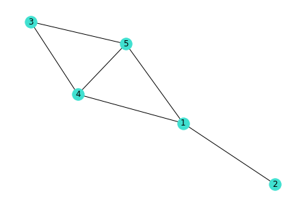
$$M=\begin{bmatrix}0&1&0&1&1\\ 1&0&0&0&0\\ 0&0&0&1&1\\ 0&0&1&0&1\\ 1&0&1&0&0\end{bmatrix}$$ (37)

Figure 1: Five-node network for simulation experiments. Left: picture of the network. Right: adjacency matrix.

We will simulate realizations from the Poisson-GNARI($1,[1]$) process with lengths $T=50,200$ and $500$ observations and repeat this $1000$ times for each choice of $T$ and estimate parameters for each realization.

$T$	$\alpha_{1}$	$\beta_{1,1}$	$\lambda$
50	0.482 (0.053)	0.370 (0.061)	14.8 (6.57)
200	0.496 (0.025)	0.392 (0.031)	11.3 (2.96)
500	0.497 (0.015)	0.397 (0.019)	10.6 (1.73)
True	0.500	0.400	10.0

Table 1: The mean (and standard deviation) over $1000$ conditional least squares estimates of each parameter in the GNARI($1,[1]$) model for each length $T$

Table 1 shows the results: the mean of the estimates clearly approaches the truth as $T$ gets larger. The standard deviation is approximately inversely proportional to $\sqrt{T}$, i,e., $\frac{\text{std}(\hat{\theta}_{T})}{\text{std}(\hat{\theta}_{m})}\approx\frac{m}{T}$, which is consistent with the asymptotic properties. It is also worth noting that there is a tendency for underestimation of $\alpha_{1}$ and $\beta_{1,1}$, but overestimation of $\lambda$.

3.2 NGNAR parameter estimation simulation study

Table 2 shows the results of a similar simulation study to the previous one, but for a NGNAR process. We simulate one hundred realizations of a Poisson-NGNAR($1,[1]$) with $g(\cdot)=\operatorname{softplus}(\cdot)$, $\alpha_{1}=0.5$, $\beta_{1,1}=-0.4$, and $\alpha_{0}=10$ for lengths $T=50,200,500$ on the same network as in the previous section. We only use $100$ realizations as NGNAR estimation is computationally intensive due to its nonlinear nature.

For each realization, we fit the NGNAR model using both conditional least squares and conditional maximum likelihood with optimisation by the ADAM optimiser from Kingma and Ba (2015) and both under TensorFlow as described in Abadi et al. (2015).

$T$	Est. Method	$\alpha_{1}$	$\beta_{1,1}$	$\alpha_{0}$
50	CLS	0.493	-0.407	10.2
		(0.058)	(0.067)	(1.14)
	CMLE	0.493	-0.404	10.2
		(0.053)	(0.065)	(1.05)
200	CLS	0.504	-0.399	9.92
		(0.029)	(0.039)	(0.639)
	CMLE	0.503	-0.400	9.96
		(0.027)	(0.037)	(0.622)
500	CLS	0.500	-0.397	9.96
		(0.018)	(0.024)	(0.382)
	CMLE	0.500	-0.397	9.97
		(0.018)	(0.021)	(0.365)
True		0.500	-0.400	10

Table 2: The mean (and standard deviation) across the 100 conditional least squares and conditional MLE estimates for each parameter in the Poisson-NGNAR($1,[1]$) model for each length $T$.

3.3 Predictive comparison via simulation

We compare our new GNARI and NGNAR models with the recent PNAR count network time series model of Armillotta and Fokianos (2024) via simulation. Using the same network as earlier (as shown in Figure 1) we simulate $500$ realizations of length $T=500$ from each of the following processes

P1

Poisson-GNARI(1,[1]) with $\alpha_{1}=0.5$, $\beta_{1,1}=0.4$, and $\alpha_{0}=10$;

P2

Poisson-NGNAR(1,[1]) with $g(\cdot)=\operatorname{softplus}(\cdot)$, $\alpha_{1}=0.5$, $\beta_{1,1}=0.4$, $\alpha_{0}=10$;

P3

Poisson-NGNAR(1,[1]) with $g(\cdot)=\operatorname{softplus}(\cdot)$, $\alpha_{1}=0.1$, $\beta_{1,1}=-0.8$, $\alpha_{0}=10$;

P4

PNAR(1) with $\alpha_{1}=0.5$, $\beta_{1}=0.4$, $\beta_{0}=10$.

For each simulated realisation, we fit the following models: (A) GNARI($1,[1]$), (B) NGNAR($1,[1]$) fitted by conditional least squares and (C) by conditional maximum likelihood, (D) PNAR($1,[1]$).

For this study we are interested in how well the models perform in terms of predictive performance. To do this, we divide each network time series into a training set of length $450$ and a test set of length $50$. We fit (A) to (D) on the training set, and then make a prediction of length 50, which is then compared to the test values and is assessed using mean-squared prediction error (MSPE).

	Simulated Process
	P1	P2	P3	P4
A	68.6	100.2	9.1	98.2
B	68.6	100.2	5.9	98.2
C	68.7	100.2	5.9	98.2
D	68.8	100.2	9.01	98.3

(a) $T=1$

	Simulation Process
	P1	P2	P3	P4
A	119.3	173.6	9.1	166.9
B	119.3	173.6	8.5	167.0
C	119.3	173.6	8.5	166.9
D	119.9	173.8	9.7	167.4

(b) $T=10$

	Simulated Process
	P1	P2	P3	P4
A	145.0	209.5	9.08	211.0
B	145.0	209.5	8.96	211.0
C	145.1	209.4	8.96	211.0
D	145.2	209.7	9.08	211.8

(c) $T=50$

Table 3: Average mean-squared prediction error (MSPE) between the predicted next $T$ days time series by each model (A, B, C, D) fitted to training realizations from simulated processes P1, P2, P3 and P4 on the training set evaluated on the test set over 500 realizations from each simulated model.

Table 3 shows that for the simulated GNARI, NGNAR with positive parameters and PNAR processes, all four methods have almost equal performance with the PNAR model perhaps slightly worse than the others. For the NGNAR simulation with $\beta_{1,1}=-0.8$, the NGNAR models definitively predict better than the other models, especially over the short term. However, for longer horizons there is not much to choose between the methods.

The NGNAR model is clearly more flexible than the GNARI model and the PNAR model as it can cope with negative parameters. In principle, the log-linear version of the Armillotta and Fokianos (2024) model can cope with negative parameters. However, the error structure that the log-linear model assumes is different to that of the simulated processes P1–P4 above. To avoid doubt we repeated the simulation/prediction exercise above for the log-linear model and the prediction errors were uniformly at least four times worse than those reported in Table 3 and, in many cases, much worse.

GOT HERE

4 Example: New York State COVID forecasting

4.1 Data description

We obtained daily counts of people who tested positive for COVID19 in the 62 counties of New York State, USA from New York State Department of Health (2022) during the period 1st March 2020 to 23rd May 2022. The counts can be written as a multivariate time series of dimension $T\times N=783\times 62$ (some common missing values at the head of the time series were discarded).

Figure 2 shows a map of the counties of New York State, which are colour-coded according to the logarithm of the number of COVID positives. It can be seen that the highest count is centred in and around New York City at the bottom right of the map.

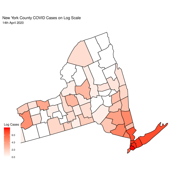
Figure 2: Counties of New York State with log COVID cases indicated by heat map.

We constructed a network for the counties by treating each county as a vertex and joining two vertices if the respective counties shared a border. Network weights are equally allocated between the neighbours (e.g. if a county has $k$ neighbours, then the out-weight of that county to each of its neighbours is $k^{-1})$. Figure 3 depicts the graph we use for our network time series modelling.

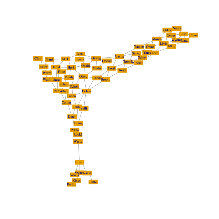
Figure 3: Graph associated with New York state counties.

The New York city area can be seen at the ‘bottom’ of the graph in Figure 3.

4.2 Prediction evaluation method

We split the multivariate time series into a training series of length $700$ and a test series of length $83$. The time series for each county follows a similar pattern, but the actual $X_{i,t}$ values are different in level. This indicates that we can use a global $\alpha$ in the model, but local values of $\lambda$ or $\alpha_{0}$ for the GNARI and NGNAR models, respectively. In other words, the $\alpha_{i,0}$ in (33) and the $\lambda_{i}$ as the expectation of the noise in (12) will both not be constant values of $i$. The autocorrelations of $\{X_{i,t}\}_{t}$ and the cross-correlations between $\{X_{i,t}\}_{t}$ and its weighted sum $\{\mathcal{N}^{(1)}(X_{i,t-\tau})\}_{t}$, $\tau=0,1,\ldots,30$ are all positive: at least for the first $30$ lags, which shows the feasibility of the GNARI model.

We will fit four model types on the training series: GNAR, PNAR, GNARI and NGNAR models. Each model will be fitted twice using maximum lags of $14$ and $21$, respectively. The order of $\alpha$, $[I_{1},\dots,I_{p}]$ where $I_{j}$ is either 1 or 0 indicating whether the autoregressive term at lag $j$ is included. The order of $\beta$, $[s_{1},\ldots,s_{p}]$, will be selected using backward deletion and the Bayesian information criterion (BIC) as the metric. For the PNAR model, the quasi-MLE fitting method provided in the PNAR package in R can only fit a PNAR(1) model for this particular dataset as higher order models will lead to a non-zero score function.

We will fit the GNAR model using conditional least squares, the GNARI model using constrained least squares to ensure that the model parameters are non-negative. The NGNAR models will be fitted using conditional MLE using the ADAM optimizer from Kingma and Ba (2015). In the GNARI model we will assume that the $\epsilon_{i,t}$ is Poisson-distributed. The NGNAR models will use the $\operatorname{softplus}$ function as the response function and Poisson as the conditional distribution.

For each model, we predict the time series for the next 83 days. Denote the predicted time series $\{\hat{X}_{i,t}^{(M)}\}_{t=701}^{783}$ where $M$ is the model. The results will be shown by plotting $\{\hat{X}_{i,t}^{(M)}\}_{t=701}^{783}$ along with the true actual values $\{X_{i,t}\}_{t=701}^{783}$ for some $i$. We will compute the mean-squared prediction error (MSPE) and mean absolute prediction error (MAPE) between the next $T$ days prediction for each model and its corresponding true value, i.e., the MSPE between $\{\hat{X}_{i,t}^{(M)}\}_{t=701}^{700+h}$ and $\{X_{i,t}\}_{t=701}^{700+h}$, for $h=1,\ldots,83$.

4.3 Results

The order selected for the GNARI($14$) and GNARI($21$) turned out to be identical, so only one GNARI result is reported here. Tables 4, 5 and Figure 4 clearly show the superiority of the NGNAR models (particularly the one of order $14$) for short- to medium-term forecasting and the GNARI model for longer terms forecasts.

	Forecast horizon $h$
Model	$1$	$5$	$10$	$25$	$50$	$83$
GNAR($14$)	3.18	7.47	6.55	36.6	163	433
GNAR($21$)	6.60	9.44	7.47	20.6	110	369
GNARI	3.25	8.20	7.98	15.5	43.4	147
NGNAR($14$)	3.85	6.25	4.53	17.9	93.7	321
NGNAR($21$)	3.97	6.33	4.53	16.5	87.3	306
PNAR($1$)	3.95	7.91	6.44	18.4	87.0	297

Table 4: The mean-squared prediction error $\times 100$ (MSPE) between the predictions up to forecast horizon $h$ (to three significant figures).

	Forecast horizon $h$
Model	$1$	$5$	$10$	$25$	$50$	$83$
GNAR($14$)	10.1	10.6	11.0	22.8	52.3	86.8
GNAR($21$)	12.9	12.4	12.2	17.3	39.6	74.5
GNARNI	10.4	13.9	14.1	18.3	26.4	45.6
NGNAR($14$)	10.0	9.66	9.23	14.9	35.1	66.5
NGNAR($21$)	10.3	9.71	9.42	14.6	33.7	64.2
PNAR($1$)	11.4	14.9	15.2	22.5	40.7	69.0

Table 5: The mean absolute prediction error (MAPE) between the predictions up to forecast horizon $h$ (to three significant figures).

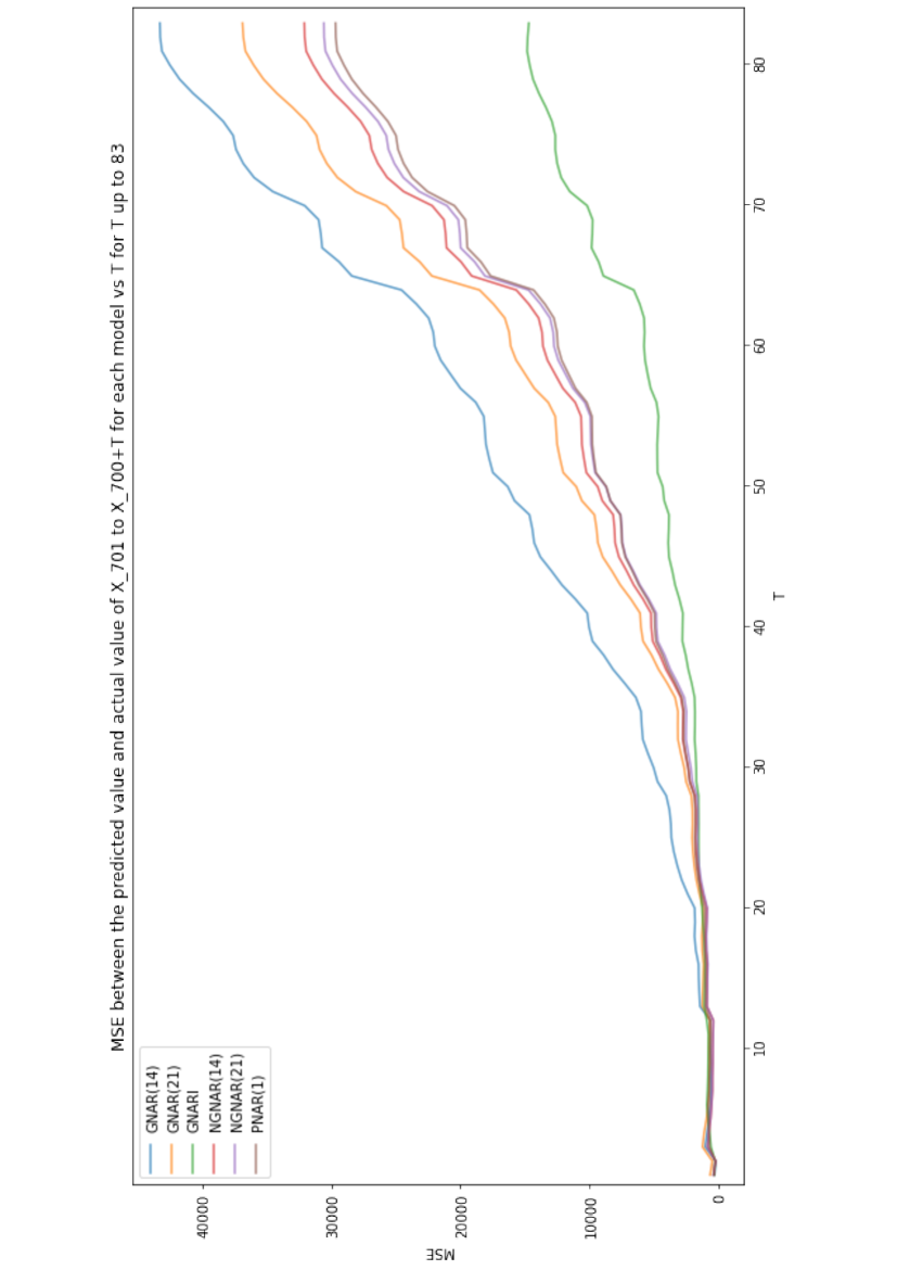
Figure 4: Plot of MAPE between the prediction of the next $h$ days time series and the corresponding true values, i.e., the aggregate MAPE between $\{\hat{X}_{i,t}^{(M)}\}_{t=701}^{700+h}$ and $\{X_{i,t}\}_{t=701}^{700+h}$, against $T$ for $T=1,\ldots,83$.

5 Discussion

This article has introduced two new models for network time series that have count data as observations. In general, the models are useful and work well achieving similar performance to PNAR models for data with positive autocorrelations. For the COVID data above the new models performed particularly well and better than PNAR and GNAR. The NGNAR model works well in estimating negative network parameters, unlike comparator models. We have established the asymptotic properties for GNARI and NGNAR processes. For the latter showing its asymptotic normality by utilising established results in this context. Moreover, we have described methods for estimation using conditional least squares and conditional maximum likelihood.

6 Acknowledgements

Li gratefully acknowledges partial support by Imperial College London. Both gratefully acknowledge support from EPSRC NeST Programme grant EP/X002195/1.

Appendix A Proofs

Proof of Lemma (2.1).

We drop the $t$ subscript for simplicity. The moment generating functions of $B_{j,r,k}$ and $Y_{i,j}^{(r)}$ are

$$M_{B_{j,r,k}}(s)=1-\beta_{j,r}+\beta_{j,r}e^{s}$$ (38)

and

$$M_{Y_{i,j}^{(r)}}(s)=\prod_{q\in{\mathcal{N}}_{t}^{(r)}(i)}(1-w_{i,q}-w_{i,q}e^{s})^{X_{q,t-j}},$$ (39)

for $s\in{\mathbb{R}}$. For the moment generating function of $Z_{i,j}^{(r)}$ we have

$$M_{Z_{i,j}^{(r)}}(u) ={\mathbb{E}}\left\{e^{uZ_{i,j}^{(r)}}\right\}$$ (40)

$$={\mathbb{E}}\left[{\mathbb{E}}\{e^{uZ_{i,j}^{(r)}}|Y_{i,j}^{(r)}\}\right]$$ (41)

$$={\mathbb{E}}\{(1-\beta_{j,r}+\beta_{j,r}e^{u})^{Y^{(r)}_{i,j}}\}$$ (42)

$$=M_{Y^{(r)}_{i,j}}\{\log(1-\beta_{j,r}+\beta_{j,r}e^{u})\}$$ (43)

$$=\prod_{q\in{\mathcal{N}}_{t}^{(r)}(i)}\{1-w_{i,q}+w_{i,q}(1-\beta_{j,r}+\beta_{j,r}e^{u})\}^{X_{q,t-j}}$$ (44)

$$=\prod_{q\in{\mathcal{N}}_{t}^{(r)}}(1-\beta_{j,r}w_{i,q}+\beta_{j,r}w_{i,q}e^{u})^{X_{q,t-j}},$$ (45)

which is the moment generating function of the Poisson binomial distribution, with the parameters specified in the statement of the lemma. By the uniqueness of MGFs, this is the distribution of the $Z^{(r)}_{i,j}$.

∎

Proof of Lemma (2.2).

We prove the result for GNARI variant (17). For $A\in\mathbb{R}^{N\times N},\mathbf{X}=(X_{1},\ldots,X_{N})\in\mathbb{R}^{N},N\in\mathbb{N}$, define $A\circ\mathbf{X}$ to be

$$A\circ\mathbf{X}=\begin{pmatrix}\sum_{k=1}^{N}[A]_{1,k}\circ X_{j}\\ \vdots\\ \sum_{k=1}^{N}[A]_{N,k}\circ X_{j}\end{pmatrix}$$ (46)

Hence, the GNARI process (17) can be viewed as a multivariate integer-valued autoregressive (MGINAR) process, see Latour (1997):

$$\mathbf{X}_{t}=\sum_{j=1}^{p}A_{j}\circ\mathbf{X}_{t-j}+\mathbf{\epsilon}_{t},$$ (47)

where $\mathbf{X}_{t}=(X_{1,t},\dots,X_{N,t})^{T}$, $A_{j}=\operatorname{diag}\{\alpha_{i,j}\}+\sum_{r=1}^{s_{j}}\beta_{j,r}W^{(r)}$ and $W^{(r)}$ is the matrix with entries

$$[W^{(r)}]_{l,m}=w_{l,m}\mathbb{I}\{m\in\mathcal{N}^{(r)}(l)\}$$

and $\mathbf{\epsilon}_{t}=(\epsilon_{1,t},\ldots,\epsilon_{N,t})^{T}$.

Let

$$A=\begin{bmatrix}A_{1}&A_{2}&\dots&A_{p-1}&A_{p}\\ I&0&\dots&0&0\\ \vdots&\vdots&\ddots&\vdots&\vdots\\ 0&0&\dots&I&0\end{bmatrix}.$$ (48)

Then, the GNARI process is equivalent to

$$\mathbf{Y}_{t}=A\circ\mathbf{Y}_{t-1}+\mathbf{e}_{t},$$ (49)

where $\mathbf{Y}_{t}=(\mathbf{X}_{t}^{T},\mathbf{X}_{t-1}^{T},\ldots,\mathbf{X}_{t-p+1}^{T})^{T}$ and $\mathbf{e}_{t}=(\epsilon_{t}^{T},0^{T},\ldots,0^{T})^{T}$.

Latour (1997) Proposition 3.1 permits us to conclude that, under the condition that all roots of $\det(I-Az)$ are outside the unit circle, or, equivalently, all eigenvalues of $A$ are inside the unit circle, the process $\{\mathbf{X}_{t}\}_{t}$ has a unique stationary solution.

Knight et al. (2020) Appendix A tells us that the above condition can be achieved if condition (19) holds. Hence, condition (19) guarantees the unique stationary solution of the GNARI process. ∎

Proof of Lemma (2.3).

Let

$$\mathbf{Y}_{t}=(X_{1,t},\ldots,X_{N,t},\ldots,X_{1,t-p+1},\ldots,X_{N,t-p+1})^{T},$$ (50)

where $A$ is the same matrix as in (48), and $g(x)=s(x)$ is the $\operatorname{softplus}$ function. Then $\{\mathbf{Y}_{t}\}_{t}$ is Markov, aperiodic and irreducible and we have

$$\mathbb{E}(\mathbf{Y}_{t}|\mathbf{Y}_{t-1})=f(A\mathbf{Y_{t-1}}),$$ (51)

where $f(\mathbf{X})=\{g(X_{1}),\ldots,g(X_{p}),X_{p+1},\ldots\}^{T}$. From Appendix A in Knight et al. (2020), we know that all eigenvalues of $A$ can be assumed to be inside in the unit circle. This is equivalent to the spectral radius of $A$, $\rho(A)<1$. Thus, by Lemma 2.5 in An and Huang (1996), there exists a matrix norm $||\cdot||_{m}$, a vector norm $||\cdot||_{v}$, and $\lambda\in(0,1)$, such that

$$||Ax||_{v}\leq||A||_{m}||x||_{v}\leq\ \lambda||x||_{v},\ \ \ \forall x\in\mathbb{R}^{Np}.$$ (52)

Now, $\forall\mathbf{y}\in\mathbb{R}^{Np}$

$$\mathbb{E}(||\mathbf{Y}_{t+1}||_{v}\,|\,\mathbf{Y}_{t}=\mathbf{y})\leq||f(A\mathbf{y})||_{v}$$ (53)

and

$$||A\mathbf{y}||_{v}\leq\ \lambda||\mathbf{y}||_{v}.$$ (54)

It is simple to show that $\lim_{x\xrightarrow{}\infty}g(x)=x$, and $|g(x)|<|x|$ for all $x<\operatorname{arcsinh}(-1/2)$, for $g(x)=s_{1}(x)$, the $\operatorname{softplus}$ function. We can thus find $C\in\mathbb{R}^{Np}$ to be $R^{Np}_{\geq 0}\bigcap C^{\prime}$ where $C^{\prime}$ is a sphere in $\mathbb{R}^{Np}$ such that if $\mathbf{y}\notin C$, the negative elements of $A\mathbf{y}$ are less than $\text{archsinh}(-1/2)$ and $||\mathbf{y}^{\prime}-A\mathbf{y}||_{v}<(1-\lambda)M/2$, where $\mathbf{y}^{\prime}$ is the vector whose non-negative entries equals that of $f(A\mathbf{y})$ and negative entries equals that of $A\mathbf{y}$, and $M=\inf_{\mathbf{y}\notin C}||Y||_{v}$.

Then $\forall\mathbf{y}\notin C$,

$$||f(A\mathbf{y})||_{v} \leq||A\mathbf{y}^{\prime}||_{v}$$

$$\leq||\mathbf{y}^{\prime}-A\mathbf{y}||_{v}+||A\mathbf{y}||_{v}$$

$$\leq(1-\lambda)M/2+\lambda||\mathbf{y}||_{v}$$

$$\leq(1/2+\lambda/2)||\mathbf{y}||_{v}$$

where clearly $1/2+\lambda/2<1$.

Now, by Lemma 2.2 from An and Huang (1996), which is a reformulation of the Tweedie’s criterion for ergodicity:

Let $\{\mathbf{Y_{t}}\}$ be aperiodic irreducible. Suppose that there exist a small set $C$, a nonnegative measurable function $g$, positive constants $c_{1}$, $c_{2}$ and $\rho<1$ such that

$$\mathbb{E}[g(\mathbf{Y_{t+1}})|\mathbf{Y_{t}}=\mathbf{y}]\leq\rho g(\mathbf{y})-c_{1},\ for\ any\ y\notin C$$ (55)

and

$$\mathbb{E}[g(\mathbf{Y_{t+1}})|\mathbf{Y_{t}}=\mathbf{y}]\leq c_{2},\ for\ any\ y\in C$$ (56)

Then $\{\mathbf{Y_{t}}\}$ is geometrically ergodic.
Also, the fact that the $\operatorname{softplus}$ function is bounded for the bounded region, we have that the Markov process $\{\mathbf{Y_{t}}\}_{t}$ is geometrically ergodic, and thus has a unique stationary solution. This implies that the NGNAR process $\{X_{t}\}_{t}$ has a unique stationary solution. ∎

References

- Abadi et al. (2015) Abadi, M., Agarwal, A., Barham, P., Brevdo, E., Chen, Z., Citro, C., Corrado, G. S., Davis, A., Dean, J., Devin, M., Ghemawat, S., Goodfellow, I., Harp, A., Irving, G., Isard, M., Jia, Y., Jozefowicz, R., Kaiser, L., Kudlur, M., Levenberg, J., Mané, D., Monga, R., Moore, S., Murray, D., Olah, C., Schuster, M., Shlens, J., Steiner, B., Sutskever, I., Talwar, K., Tucker, P., Vanhoucke, V., Vasudevan, V., Viégas, F., Vinyals, O., Warden, P., Wattenberg, M., Wicke, M., Yu, Y., and Zheng, X. (2015) TensorFlow: Large-scale machine learning on heterogeneous systems, software available from tensorflow.org.
- Al-Osh and Alzaid (1987) Al-Osh, M. A. and Alzaid, A. A. (1987) First-order autoregressive INAR(1) process, J. Time Ser. Anal., 8, 261–275.
- Alzaid and Al-Osh (1990) Alzaid, A. A. and Al-Osh, M. (1990) An integer-valued th-order autoregressive structure INAR() process, J. Appl. Prob., 27, 314–324.
- An and Huang (1996) An, H. Z. and Huang, F. C. (1996) The geometrical ergodicity of nonlinear autoregressive models, Statistica Sinica, 6, 943–956.