Efficiency of Unsupervised Anomaly Detection Methods on Software Logs

Abstract.

Software log analysis can be laborious and time consuming. Time and labeled data are usually lacking in industrial settings. This paper studies unsupervised and time efficient methods for anomaly detection. We study two custom and two established models. The custom models are: an OOV (Out-Of-Vocabulary) detector, which counts the terms in the test data that are not present in the training data, and the Rarity Model (RM), which calculates a rarity score for terms based on their infrequency. The established models are KMeans and Isolation Forest. The models are evaluated on four public datasets (BGL, Thunderbird, Hadoop, HDFS) with three different representation techniques for the log messages (Words, character Trigrams, Parsed events). We used the AUC-ROC metric for the evaluation. The results reveal discrepancies based on the dataset and representation technique. Different configurations are advised based on specific requirements. For speed, the OOV detector with word representation is optimal. For accuracy, the OOV detector combined with trigram representation yields the highest AUC-ROC (0.846). When dealing with unfiltered data where training includes both normal and anomalous instances, the most effective combination is the Isolation Forest with event representation, achieving an AUC-ROC of 0.829.

1. Introduction

Software anomaly detection is gravitating towards more complex algorithms, despite evidence suggesting that computationally intensive deep-learning approaches may not offer significant benefits (Yu et al., 2023; Wu et al., 2023; Landauer et al., 2023; Mäntylä et al., 2022; Cao and Niu, 2022; Nyyssälö et al., 2022). This study aims to examine the anomaly detection approaches that are both fast and require little preliminary effort by the log owner. Primarily this means that we are using unsupervised methods that do not require labelled anomalies in the training data. Labelling large log files is a laborious endeavor and in industrial settings the labels are rarely available (Chen et al., 2021).

A systematic literature review (Bhanage et al., 2021) shows that majority of the recent studies are based on computationally heavy approaches such as deep learning or utilize supervised models. Another literature review (Lupton et al., 2021) notes the lack of real world use-cases and reports Loglizer as the only available toolkit for log anomaly analysis. The results from the Loglizer toolkit have been reported in a previous study (Chen et al., 2021). In the study Invariant Mining reached the best results with F1-score of 0.91 on both HDFS and BGL datasets. Regarding unsupervised models, the authors note challenges of setting and testing out various thresholds (Chen et al., 2021). The Loglizer paper notes that unsupervised models are also much more time consuming than supervised ones. For example, 1.5 million lines on HDFS took over 1000 seconds with Invariant Mining.

In this paper, we examine methods that do not require labelled data with two approaches. In one, we will train the model on completely unfiltered data with both anomaly and normal data while in the other, only normal data is used for training. The difference between these two approaches has not been addressed in the prior work to our best knowledge. In the latter, anomaly detection will be based on the dissimilarity of the log messages in the test and training data. This approach has been demonstrated by previous work (Du et al., 2017), (Mäntylä et al., 2022) and is sometimes referred as ”novelty detection” (Fournier et al., 2023).

Furthermore, we examine the effect of log representation to see whether representations with lower computational cost can prove effective. A recent study (Wu et al., 2023) conducted a thorough analysis on log representations used in anomaly detection. The authors applied several classical and semantic-based representations on traditional and deep-learning models. One of the key findings was that the traditional models work better with classical representations. A widely used technique for log representation is to use a clustering, aka log parsing, algorithm, to find out the static part of a log message called the template and use that (or its ID) to represent the logline (Bhanage et al., 2021). As this step is computationally expensive we will use more straight forward approaches for representing the log messages such as word-based splitting and chracter trigram generation to assess their effect on the performance of the selected models. We formulated the following research questions:

• RQ1: How good are the unsupervised models for anomaly detection as measured with AUC-ROC and time?

• RQ2: How does log representation affect the results: Words vs. trigrams vs. event ID?

• RQ3: Do the models perform better after filtering out anomalies from the training data?

2. Research methods

This chapter describes the preprocessing, datasets, metrics and models used in the study. Our environment consists of a virtual machine that has Intel Core Processor (Broadwell, IBRS) with 28 cores at 2,4 Ghz and 224 GB of memory. The replication package will be available at GitHub .

2.1. Preprocessing

The data was loaded directly from raw log files to Polars dataframes. Next, the log messages are normalized to reduce the effect of parameters (non-static parts of the message). However, due to placing strong emphasis on performance time we only perform three operations with fast Polars-native string operations: (1) Convert all letters to lowercase, (2) Replace every numeral with the digit ’0’, (3) Reduce any consecutive series of zeros to a single ’0’. For example, the string ”Time 12:34:56” would be converted to ”time 0:0:0”. When it comes to words and trigrams, normalization will make the resulting vocabulary smaller. While the primary reason for this is to improve the accuracy due to minimazing the effect of parameters, smaller vocabulary also makes the model faster.

The normalized log messages are transformed into event IDs or lists consisting of trigrams (i.e., three consecutive letters) or words. Event IDs are created with the Drain parser (He et al., 2017). Words are extracted with a Polars native string split by using whitespace as the separator.

The data is then divided into training and test sets based on proportion defined in Table 1. From the training set, we create two instances: One with full data and another where anomalies are filtered out. These will be referred as the unfiltered and filtered setups respectively. Finally these sets are turned into matrices with the TfidfVectorizer (Pedregosa et al., 2011). Tf-idf is a common technique for feature extraction that adds weight to the most important tokens.

2.2. Datasets

The datasets used in the study are BGL (Oliner and Stearley, 2007), Thunderbird (Oliner and Stearley, 2007), HDFS (Xu et al., 2009) and Hadoop (Lin et al., 2016), which are easily accessible via LogHub (He et al., 2020). Table 1 shows the summary of the datasets. BGL and Thunderbird are missing the rows for number of sequences as they do not have them and they are labeled at line level. Similarly, the number of normal log lines cannot be determined for HDFS and Hadoop because they are labeled on the sequence level.

The most significant difference with the sequence and event based datasets for anomaly detection is that when using event ID as the log representation, the sequence based datasets have multiple IDs to influence the prediction while event based ones only have one. For word- and trigram-representations, the sequence based datasets are handled by flattening the lists of lists into a single list with a single anomaly label.

We generally wanted to use the same settings for all datasets which means using all data and a small split for training. DeepLog has demostrated that for HDFS a less than 1% split for training is sufficient (Du et al., 2017). To play it safe we went with a little higher 5% for everything except Hadoop which has a very small number of sequences. Due to memory constraints we also had to represent Thunderbird with a randomly chosen 10% sample of the whole data. The sample is still over 20 million lines. For Thunderbird, the 5% training data is taken from this sample, so in effect, the training data is just 0.5% of the total data.

2.3. Metrics

AUC-ROC (Bradley, 1997) is a combination of the abbreviations Area Under Curve (AUC) and Receiver Operating Characteristic (ROC). ROC curve is a plot of the true positive rate against the false positive rate across a range of thresholds. With AUC we refer to the area under this curve. This area goes from 0 to 1 and in practice it means the probability that a randomly selected positive sample is ranked highed than a negative one (Bradley, 1997).

The main reason for utilizing AUC-ROC in this study is that it is not dependent on a threshold. With supervised models you could assess the model specific anomaly scores in relation to the labels and adjust the threshold accordingly. In unsupervised models this is not possible which leads to subjective threshold selection.

The model execution time is reported as the total of training and predicting with a given model. Preprocessing times will be reported separately as it consists of several stages where some are mandatory for all models and others are not.

Table 1. Data summary

Dataset	HDFS	BGL	Hadoop	Thunderbird
Log lines	11,175,629	4,747,963	394,308	211,212,174
Normal seq	558,223	-	11	-
Ano seq	16,838	-	43	-
Normal lines	-	4,399,503	-	193,744,715
Ano lines	-	348,460	-	17,467,459
Data used	100%	100%	100%	10%
Train portion	5%	5%	50%	5%

2.4. Models

We did initial tests on several models but some well-known unsupervised models were found to be too slow, such as the Local Outlier Factor and One-class SVM. Additionally, we created two simple custom models, Out-of-vocabulary Detector and a Rarity Model, as we suspected they would be competitive against the established models at least in terms of execution speed.

2.4.1. Out-of-vocabulary Detector

We started to design the Out-of-vocabulary Detector (OOVD) as a tool for aiding other models. However, when training the model with only normal data OOV terms are great candidates for being anomalies. As such the OOVD by itself can produce good results on simple datasets. It is important to note that the OOVD can not work if there are anomalies in the training data vocabulary so it will only be used with the filtered setup. For other models the anomalousness of a term is determined by its relation to other terms, but OOVD only checks whether it belongs to a set. Therefore, if the set is created randomly the results will be random as well.

Counting OOV terms in millions of lists individually would be a slow operation so we utilize a strategy that takes advantage of the way OOV terms are handled by vectorizers. When transforming the test data with CountVectorizer that was fitted with training data, the OOV terms will automatically get the value 0. Then we can simply subtract the in-vocabulary terms calculated by the CountVectorizer from the total numbers of terms to get the number of OOV terms. Working with total counts as such can be hundreds of times faster than matching the words individually in a for-loop.

2.4.2. Isolation Forest

The first model implemented with Sklearn (Pedregosa et al., 2011) is Isolation Forest (IF). It is based on random isolation of features and splitting between maximum and minimum values of selected feature (Pedregosa et al., 2011). Due to their nature, anomalies are easier to separate than normal data. Based on that, it can be determined that the number of partitions it takes to isolate a data point corresponds with how likely it is to be normal.

2.4.3. KMeans

The second model implemented with Sklearn is the KMeans clustering algorithm (Pedregosa et al., 2011). It works by starting with random centroids and assigning data points to the closest one. As data is added, the centroids are updated based on the mean of all the data points in that centorid. The trained model should have clearly defined clusters around the centroids. For prediction, we give the anomaly score as the minimum distance from the nearest centroid.

2.4.4. Rarity Model

We implemented a simple class based on negative logarithm that we called the Rarity Model (RM). In essence, negative logarithm measures the relative infrequency of individual terms in the data that increases based on their rarity. For implementation, the rarity scores are first precalculated for each term in the training data and assigned into a vector. Next, the dot product of the precalculated vector and the sparse matrix generated by the Tf-idf vectorizer from the test data is calculated. The total rarity score for the log message will be the dot product divided by the total number of terms in the message. Given its simple design and reliance on pre-built matrix multiplication routines, the RM is anticipated to function with remarkable speed.

3. Results

3.1. AUC-ROC results

Table 2. AUC with unfiltered training data

Log rep.	Model	BGL	Tb	Hadoop	HDFS	Avg
Words	IF	0.672	0.783	0.611	0.990	0.764
	KMeans	0.722	0.293	0.579	0.971	0.641
	RM	0.638	0.217	0.365	0.999	0.555
Trigrams	IF	0.675	0.814	0.698	0.981	0.792
	KMeans	0.741	0.166	0.611	0.956	0.619
	RM	0.735	0.102	0.540	0.999	0.594
Events	IF	0.755	0.693	0.889	0.978	0.829
	KMeans	0.766	0.187	0.847	0.984	0.696
	RM	0.581	0.222	0.486	0.929	0.555

Table 3. AUC with filtered (normal only) training data

Log rep.	Model	BGL	Tb	Hadoop	HDFS	Avg
Words	OOVD	0.777	0.802	0.786	0.543	0.727
	IF	0.482	0.433	0.611	0.954	0.620
	KMeans	0.937	0.893	0.579	0.940	0.837
	RM	0.958	0.967	0.381	0.950	0.814
Trigrams	OOVD	0.997	0.997	0.845	0.545	0.846
	IF	0.605	0.530	0.845	0.944	0.731
	KMeans	0.945	0.582	0.802	0.953	0.820
	RM	0.988	0.714	0.619	0.982	0.826
Events	OOVD	0.995	0.895	0.903	0.535	0.832
	IF	0.004	0.104	1.000	0.937	0.511
	KMeans	0.041	0.235	0.806	0.981	0.515
	RM	0.405	0.387	0.278	0.840	0.477

The results for AUC-ROC are showcased in Table 2 and Table 3. It is apparent that there is no single model-representation pair that gets the best results on each dataset. IF is a strong candidate for the best model if one only has unfiltered data contain both anomalies and normal observations without labels. KMeans performs similarly to IF on other datasets but fails completely on Thunderbird. RM performs poorly on the unfiltered setup as is to be expected due to the anomalies being in the vocabulary. The reason RM gets a good score with unfiltered HDFS is that the dataset just has little anomalies in general so when RM sees something rare it will get a higher anomaly score.

With the filtered (normal only) setup both KMeans and RM improve the results drastically when using the word- or trigram-representation. It is easy to intuitively understand why this happens on the RM. As the vocabulary only consists of what is normal, the model learns what is normal and deviations from that can be considered abnormal, not just rare. It is interesting that the performance went down with the filtered training data on both the IF model and the event-representation. Naturally, predicting based on the event ID introduces a lot of variation as BGL and Tb only have one item to predict with due to being event level labeled. Additionally, the modest preprocessing regexes might affect the parsing accuracy. Yet OOVD still managed to get good results with the events on BGL and Tb. This could suggest that the parser works well but other models are not able to handle the OOV events well.

The OOVD did well for everything except HDFS. This is likely due to the nature of the data. If we observe the values that OOVD and RM get, it is usually the case that when one does relatively well, the other does relatively worse. This is caused by the fact that RM (along with IF and Kmeans) do not have a way of distinguishing between OOV terms and other zeros in the matrices. In practice, the question that flips the balance is whether the term is never seen or very rarely seen. On BGL-trigrams both the RM and OOVD get great results which suggests that the anomalous log messages have both OOV and very rare terms in them. An example of this could be a folder path as the hierarchical structure goes from generic to rare by its nature. The folder example also explains why the OOVD did worse on the word-representation. As the words are not separated by slashes, the whole path becomes a long word that is likely to increase the anomaly score.

3.2. Time results

Table 4. Time with filtered training data (s)

Log rep.	Model	BGL	Tb	Hadoop	HDFS	Avg
Words	OOVD	1.29	5.30	¡ 0.01	0.20	1.70
	IF	34.00	185.87	0.13	9.49	57.37
	KMeans	2.58	13.97	0.31	0.53	4.35
	RM	1.62	9.27	¡ 0.01	0.19	2.77
Trigrams	OOVD	2.96	34.53	¡ 0.01	0.36	9.46
	IF	93.24	999.70	0.15	48.46	285.39
	KMeans	4.16	25.35	0.03	1.61	7.79
	RM	2.02	11.66	0.01	0.43	3.53
Events	OOVD	0.74	4.31	¡ 0.01	0.18	1.31
	IF	21.90	106.43	0.17	4.53	33.26
	KMeans	2.17	10.56	0.03	0.48	3.31
	RM	1.37	7.83	0.01	0.23	2.36

There were no substantial differences between the runtimes on the unfiltered and filtered setups. Table 4 show that OOVD and RM are generally the two fastest approaches with KMeans being a little slower. Depending on the data size and use case, IF can become unfeasible due to the low speed. For example, with the trigram-representation IF could be 100 times slower than RM on certain datasets. Regarding log representation, the runtime is dependent on the number of items in the data. Therefore, trigrams are the slowest while events are the fastest.

If we account for pre-processing as shown in Table 5, it becomes apparent that the word-representation is the fastest end-to-end approach when starting with a raw log file. Generating trigrams turns out to be a slow process with the standard Python tools. In fact, it was slower than the parser. However, at the time of writing there is a pull request in Polars GitHub that will improve trigram generation likely making the speed closer to word creation speed.

Table 5. Pre-processing times (s)

Time to…	Hadoop	BGL	HDFS	Tb
Load	2.77	7.86	24.71	372.24
Normalize	4.47	13.73	117.90	89.52
Create trigrams	9.50	142.58	378.16	861.33
Create words	0.38	1.83	9.03	15.80
Parse event IDs	4.69	137.18	273.67	716.53

4. Discussion

RQ1 regarded the AUC-ROC and time performance. As the results indicate, OOVD reached the best overall AUC-ROC score despite failing on HDFS. Timewise OOVD also performed the best with RM as a close second. In general the times seemed to better than suggested by previous work (Chen et al., 2021). For RQ2, we examined the log representation and found that trigram-representation can reach the best results but it is computationally much more expensive than the word-representation. Finally, for RQ3 we studied the impact of filtering out anomalies from the training data. It improved the overall results except for the IF model and the event-representation. In fact, IF model with events had the best average results for unfiltered training data and OOVD with trigrams for filtered data.

One of the key contributions of this study is the insight on the characteristics of common benchmark datasets. For example, the performance of the OOVD tells how reliant the data is on being able to detect new items, or in other words, perform novelty detection. The high scores on BGL and Tb with the OOVD essentially suggest that novelty detection is all you need with these event-level supercomputer logs. Conversely, on HDFS the other models performed much better, so there novelty detection has little value. In fact, for HDFS you only need to find the rare instances of words and the sequence is likely to be anomalous making RM the best choice.

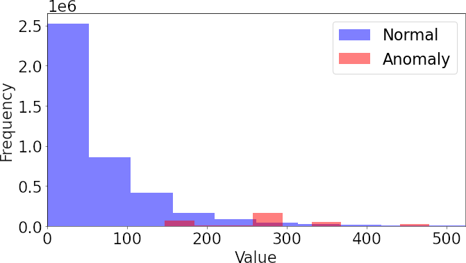
Figure 1. Distribution of the RM scores on BGL (Word-representation, filtered setup)

By using the AUC-ROC metric this study sheds light on methods that show potential but might have difficulty setting a threshold for anomaly detection. Figure 1 illustrates the distribution of RM scores for BGL using the word-representation. What the figure shows is that if we could assign a single value which would split the blue and red areas completely, we would have a perfect classifier. We can use such figures for aiding threshold selection. Of course in a real use case you would not see the colours.

Consider visualizing both red and blue bars as black in Figure 1 and observe the significant gap between them, particularly the one occurring near 250. This gap represents an ideal point for setting a threshold. If we set the threshold at 250 as suggested by the figure we would get an accuracy of 0.957 and an F1-score of 0.721.

This study opens various directions for future research. For example, finding a way to combine OOVD and with other models in a way that they do not clash with each others’ results has the promise to reach top scores on each dataset. The premise of this paper, fast and unsupervised anomaly detection, in itself encourages further studies to move toward more practical application of the anomaly detection approaches.

As a limitation of the study, parameters are very crucial on unsupervised methods but systematic parameter optimization for the models was not in the scope of this paper. Additionally, the lack of F1-score as a metric means that the results are not directly comparable with similar previous studies (Chen et al., 2021), (Meng et al., 2019).

5. Conclusion

This paper investigates speed and performance of anomaly detection using unlabeled data. Our findings indicate that our simple custom models (OOVD and Rarity Model) outperform established models (KMeans and IF) in terms of speed. In terms of performance (AUC-ROC), IF emerges as a viable option when dealing with unfiltered training data comprising both normal instances and anomalies. OOVD appears to be the preferred choice when the training data exclusively contains normal data. However, caution is advised since even the top-performing models exhibit subpar performance in certain scenarios. Nevertheless, these insights offer a good starting point for those aiming to conduct fast, unsupervised anomaly detection.

References

- Yu et al. (2023) B. Yu, J. Yao, Q. Fu, Z. Zhong, H. Xie, Y. Wu, Y. Ma, and P. He, “Deep learning or classical machine learning? an empirical study on log-based anomaly detection,” in 2024 IEEE/ACM 46th International Conference on Software Engineering (ICSE). IEEE Computer Society, 2023, pp. 392–404.
- Wu et al. (2023) X. Wu, H. Li, and F. Khomh, “On the effectiveness of log representation for log-based anomaly detection,” Empirical Software Engineering, vol. 28, no. 6, oct 2023.
- Landauer et al. (2023) M. Landauer, S. Onder, F. Skopik, and M. Wurzenberger, “Deep learning for anomaly detection in log data: A survey,” Machine Learning with Applications, vol. 12, p. 100470, 2023.
- Mäntylä et al. (2022) M. Mäntylä, M. Varela, and S. Hashemi, “Pinpointing anomaly events in logs from stability testing – n-grams vs. deep-learning.” arXiv, 2022. [Online]. Available: https://arxiv.org/abs/2202.09214
- Cao and Niu (2022) Q. Cao and H. Niu, “Higher-order markov graph based bug detection in cloud-based deployments,” in 2022 IEEE International Performance, Computing, and Communications Conference (IPCCC). IEEE, 2022, pp. 153–160.
- Nyyssälö et al. (2022) J. Nyyssälö, M. Mäntylä, and M. Varela, “How to configure masked event anomaly detection on software logs?” in 2022 IEEE International Conference on Software Maintenance and Evolution (ICSME). IEEE, 2022, pp. 414–418.
- Chen et al. (2021) Z. Chen, J. Liu, W. Gu, Y. Su, and M. R. Lyu, “Experience report: deep learning-based system log analysis for anomaly detection,” arXiv preprint arXiv:2107.05908, 2021.
- Bhanage et al. (2021) D. A. Bhanage, A. V. Pawar, and K. Kotecha, “It infrastructure anomaly detection and failure handling: A systematic literature review focusing on datasets, log preprocessing, machine & deep learning approaches and automated tool,” IEEE Access, vol. 9, pp. 156 392–156 421, 2021.
- Lupton et al. (2021) S. Lupton, H. Washizaki, N. Yoshioka, and Y. Fukazawa, “Literature review on log anomaly detection approaches utilizing online parsing methodology,” in 2021 28th Asia-Pacific Software Engineering Conference (APSEC), 2021, pp. 559–563.
- Du et al. (2017) M. Du, F. Li, G. Zheng, and V. Srikumar, “Deeplog: Anomaly detection and diagnosis from system logs through deep learning,” in Proceedings of the 2017 ACM SIGSAC Conference on Computer and Communications Security, ser. CCS ’17. New York, NY, USA: Association for Computing Machinery, 2017, p. 1285–1298. [Online]. Available: https://doi.org/10.1145/3133956.3134015
- Fournier et al. (2023) Q. Fournier, D. Aloise, and L. R. Costa, “Language models for novelty detection in system call traces,” 2023.
- He et al. (2017) P. He, J. Zhu, Z. Zheng, and M. R. Lyu, “Drain: An online log parsing approach with fixed depth tree,” in 2017 IEEE International Conference on Web Services (ICWS), 2017, pp. 33–40.
- Pedregosa et al. (2011) F. Pedregosa, G. Varoquaux, A. Gramfort, V. Michel, B. Thirion, O. Grisel, M. Blondel, P. Prettenhofer, R. Weiss, V. Dubourg, J. Vanderplas, A. Passos, D. Cournapeau, M. Brucher, M. Perrot, and E. Duchesnay, “Scikit-learn: Machine learning in Python,” Journal of Machine Learning Research, vol. 12, pp. 2825–2830, 2011.
- Oliner and Stearley (2007) A. Oliner and J. Stearley, “What supercomputers say: A study of five system logs,” in 37th Annual IEEE/IFIP International Conference on Dependable Systems and Networks (DSN’07), 2007, pp. 575–584.
- Xu et al. (2009) W. Xu, L. Huang, A. Fox, D. Patterson, and M. I. Jordan, “Detecting large-scale system problems by mining console logs,” in Proceedings of the ACM SIGOPS 22nd Symposium on Operating Systems Principles, ser. SOSP ’09. New York, NY, USA: Association for Computing Machinery, 2009, p. 117–132. [Online]. Available: https://doi.org/10.1145/1629575.1629587
- Lin et al. (2016) Q. Lin, H. Zhang, J.-G. Lou, Y. Zhang, and X. Chen, “Log clustering based problem identification for online service systems,” in 2016 IEEE/ACM 38th International Conference on Software Engineering Companion (ICSE-C). IEEE, 2016, pp. 102–111.
- He et al. (2020) S. He, J. Zhu, P. He, and M. R. Lyu, “Loghub: a large collection of system log datasets towards automated log analytics,” arXiv preprint arXiv:2008.06448, 2020.
- Bradley (1997) A. P. Bradley, “The use of the area under the roc curve in the evaluation of machine learning algorithms,” Pattern Recognition, vol. 30, no. 7, pp. 1145–1159, 1997. [Online]. Available: https://www.sciencedirect.com/science/article/pii/S0031320396001422
- Meng et al. (2019) W. Meng, Y. Liu, Y. Zhu, S. Zhang, D. Pei, Y. Liu, Y. Chen, R. Zhang, S. Tao, P. Sun, and R. Zhou, “Loganomaly: Unsupervised detection of sequential and quantitative anomalies in unstructured logs,” in Proceedings of the 28th International Joint Conference on Artificial Intelligence, ser. IJCAI’19. AAAI Press, 2019, p. 4739–4745.