Numerical approximation of Dynkin games with asymmetric information
Abstract.
We propose an implementable, feedforward neural network-based structure preserving probabilistic numerical approximation for a generalized obstacle problem describing the value of a zero-sum differential game of optimal stopping with asymmetric information. The target solution depends on three variables: the time, the spatial (or state) variable, and a variable from a standard -simplex which represents the probabilities with which the possible configurations of the game are played. The proposed numerical approximation preserves the convexity of the continuous solution as well as the lower and upper obstacle bounds. We show convergence of the fully-discrete scheme to the unique viscosity solution of the continuous problem and present a range of numerical studies to demonstrate its applicability.
1. Introduction
We consider the generalized obstacle problem
| (1.1) |
where , and is the set of -valued vectors of probabilities (see below for a detailed explanation). Furthermore, , where the coefficient functions , , as well as the barrier functions and the terminal condition are given. The mapping enforces the convexity of the solution with respect to the probability variable and is given as
where denotes the set of matrices that are symmetric and denotes the tangent cone to at ; i.e., .
Under suitable assumptions on the problem’s data, it is shown in [14, Theorem 3.4] that 1.1 admits a unique viscosity solution in the class of bounded, uniformly continuous functions that are Lipschitz-continuous and convex with respect to . The viscosity solution identifies with the value of a zero-sum game of optimal stopping (Dynkin game) with asymmetric information. More precisely, given a stochastic basis , with the augmented canonical filtration generated by an -valued Brownian motion , operator is the so-called Dynkin operator associated to the Itô-process defined on and satisfying
| (1.2) |
Consider then the zero-sum game of optimal stopping in which – under a given scenario selected randomly with probability at time – two players decide to stop the evolution of the process in order to optimize the performance criterion:
| (1.3) |
Exercising a stopping rule , Player 1 pays Player 2 the random amount , while stopping at time , Player 2 receives the random payoff . Finally, if neither of the players has stopped before the final maturity , then both players receive the amount . Clearly, Player 1 aims at minimizing (1.3), while Player 2 at maximizing (1.3). The asymmetric information feature of the game arises because only one player knows the exact scenario under which the game is played - and therefore the realized values of the game’s payoffs – while the other player is informed only about the probability according to which each of the possible scenarios is selected.
Zero-sum games of optimal stopping have been proposed by E.B. Dynkin in 1967 (see [10]) as an extension of problems of optimal stopping. Since their introduction a large number of contributions using probabilistic and/or analytic techniques arose, with the main aim of proving existence of a value for the game and a characterization of the (Stackelberg) equilibrium stopping times. We refer to the introduction of [14] for a detailed literature review. In particular, Dynkin games have received increasing attention in the mathematical finance literature since the work by Y. Kifer [17], where it is shown that zero-sum games of optimal stopping provide the fair value of the so-called Game or Israeli Options.
The literature on Dynkin games with asymmetric information is quite recent and still only counts a very limited number of contributions. Other than [14], we like to refer to [21], where the value and the equilibrium strategies of a zero-sum game of optimal stopping have been constructed in the case in which both players have different knowledge about the occurrence of a default. In [11], it is considered a zero-sum game of optimal stopping where the payoffs depend on two independent continuous-time Markov chains, the first Markov chain being observed only by Player 1, the second Markov chain being observed only by Player 2. This in particular implies asymmetric information, in the sense that players employ stopping rules that are stopping times with respect to different filtrations. More recently, in a very general not necessarily Markovian setting, it is proved in [9] that continuous-time zero-sum Dynkin games with partial and asymmetric information admit a value in randomized stopping times. As a byproduct, existence of equilibrium strategies for both players are also shown to exist. Finally, explicit results via free-boundary methods have been obtained in [8] for a class of games in which the players have asymmetric information regarding the drift of the one-dimensional diffusion underlying the game.
Concerning the numerical approximation of games with asymmetric information we refer to [3], [13] and the references therein. Furthermore, we mention [16] which studies probabilistic neural network approximations schemes for obstacle problems arising from game theory (with complete and symmetric information).
In the current paper we propose a structure-preserving probabilistic numerical approximation of (1.1). Following [3], we combine the time-discretization with a convexity-preserving discretization in the probability variable. Furthermore, we introduce a neural network approximation in the spatial variable to obtain an implementable numerical scheme and show its convergence to the viscosity solution to (1.1). We present numerical studies where we compare the the proposed neural network-based algorithm to a semi-Lagrangian scheme with piecewise linear interpolation in the spatial variable. Furthermore, we demonstrate the ability of the proposed numerical approximation to capture the expected structure of free boundaries arising in the problem of pricing Israeli -penalty put option (cf. [18], [19] among others) with asymmetric information.
The paper is organized as follows. The notation and preliminaries are introduced in Section 2. In Section 3 we introduce the semi-discrete and the fully-discrete probabilistic numerical approximation schemes and show their convergence to the viscosity solution of (1.1). Sections 4 and 5 contain auxiliary results needed for the convergence of the semi-discrete scheme: in Section 4 we discuss regularity properties of the semi-discrete numerical solution and in Section 5 we show that the accumulation points of the semi-discrete numerical approximation satisfy the viscosity sub- and supersolution properties. Numerical experiments are presented in Section 6.
2. Notation and preliminaries
2.1. Notation
We list here some notation in complement to those introduced in Section 1:
-
•
Let . For any , we denote the Euclidean norm of by
-
•
For any Lipschitz continuous function , we denote the Lipschitz coefficient by
-
•
A continuous function is said to be bounded if the norm
is finite.
-
•
For , we denote by the set of -stopping times with values in . The subset of stopping rules will be denoted by
We will frequently use the fact that the maps and satisfy for every and in the following inequalities
| (2.1) | ||||
| (2.2) |
2.2. Assumptions and viscosity solution
The following assumptions will be assumed to hold for the data in 1.1:
-
(
The functions , , , , and are uniformly Lipschitz continuous and uniformly bounded.
-
(
Furthermore, for all , we have that
-
(
We assume that, , , for some bounded domain of .
Definition 2.1 (Viscosity solution).
A function is a viscosity solution to 1.1 if the following two properties hold:
Under the assumptions (,(, the existence of a unique viscosity solution to 1.1 in the sense of the above definition is guaranteed by the next theorem, cf. [14, Theorem 3.4].
Theorem 2.2.
There exists a unique viscosity solution to 1.1 in the class of bounded uniformly continuous functions, which are convex and uniformly Lipschitz in .
3. Numerical approximation
In Section 3.1 we introduce a probabilistic numerical numerical scheme which is discrete in time and in the probability variable. We combine the semi-discrete scheme with a neural network approximation in the spatial variable to obtain a fully discrete numerical approximation in Section 3.2.
3.1. Semi-discrete numerical approximation in and
For we consider an equidistant partition , of the time interval with time-step . We define the Euler approximation of the stochastic process 1.2 over the time interval as
| (3.1) |
where are -valued i.i.d. random variables with zero mean and unit variance.
For the discretization with respect to the probability variable we adopt the approach of [3]. To this end we consider a family of regular partitions of into open simplices with mesh-size such that . The set of vertices of all is denoted by .
Given the step size we introduce the following semi-discrete numerical scheme:
-
•
For define the map as
(3.2) -
•
For proceed as follows:
-
For define the map as
(3.3) -
For , determine the map as
(3.4)
-
We note that for , the lower convex envelope in 3.4 is the solution of the minimization problem (cf. [6])
| (3.5) |
Following [3] we consider the (convexity preserving) data-dependent simplicial partition of with nodes such that the piecewise linear interpolant of the data values at the nodes over the partition (for precise definition see 3.7 below) agrees with the discrete data values . We note that the partition does not necessarily coincides with the original mesh .
We consider the set of piecewise linear Lagrange basis functions associated with the set of nodes of the partition . We recall the following properties of the Lagrange basis functions which will be frequently used throughout the paper: (a) , where is the Kronecker delta, and (b) for . We note that (a) implies that at any point there are at most basis functions with nonzero value; hence the sum in (b) reduces to .
For , , we define the piecewise linear interpolant of the discrete lower convex envelope over the convexity preserving partition as
| (3.6) |
where is the index of in ; i.e., for some , cf. [3].
Note that for each there exist at most non-zero basis functions (i.e., the basis functions associated with the vertices of the simplex for which ) with nonzero value which we denote by such that (3.6) is equivalent to
| (3.7) |
moreover
| (3.8) |
Next, we define for every
| (3.9) |
Theorem 3.1.
Proof.
We verify that that the sequence satisfies the assumptions of the Arzelà–Ascoli theorem, cf. [26, Section III.3]. The equiboundedness follows by Lemma 4.1 and the equicontinuity by Lemmas 4.1, 4.3 and 4.4. Hence, up to a subsequence, on every compact subsets of , the sequence converges uniformly to a limit that is bounded, uniformly continuous and is convex and uniformly Lipschitz continuous in .
By Proposition 5.1 (resp. Proposition 5.4), satisfies the viscosity sub- and super-solution property, hence it is a viscosity solution of 1.1 in the sense of Definition 2.1.
By Theorem 2.2, the viscosity solution of 1.1 is unique in the class of bounded, uniformly continuous functions, which are convex and uniformly Lipschitz in . Since every limit of is bounded, uniformly continuous and convex and uniformly Lipschitz in , the limit is unique.
∎
3.2. Fully discrete approximation and convergence
Below we describe a modification of the numerical scheme 3.2-(3.4) which employs a feedforward neural network approximation in the state variable . The resulting fully-discrete algorithm 3.15-3.18 is practically implementable.
To describe the neural network approximation scheme we loosely follow the exposition of [4, 16]. Typically a continuous function can be expanded in terms of a linear combination of fixed nonlinear basis functions and take the form
| (3.10) |
where are called input variables, is a set of numbers called parameters, and the target variables (the function we want to predict or approximate). The idea behind neural networks is to extend 3.10 with basis functions that depend on a linear combination of the inputs, where the coefficients in the linear combination are adaptive parameters.
Depending on the nature of the input and the assumed distribution of the target variables it is possible to generate a number of neural networks expansions of different characteristics. We are interested on the so-called Feedforward Neural Network for standard regression problems. It can be described as a series of layers of functional transformations. Each subsequent layer has a connection from the previous layer. In the first layer or input layer, we take the image of the input variable through an affine transformation that takes the form
| (3.11) |
We shall refer to the parameter as the weight matrix and the parameter as the bias vector. The superscript indicates that the corresponding parameters are in the first layer of the network. Next, a differentiable, nonlinear activation function acts component-wise on the activation vector 3.11 and transforms it into a vector of hidden units that constitutes the second layer of the neural network also know as hidden layer. Finally, we take the image of the vector of hidden unit vector through another affine transformation to get a scalar-valued output variable
| (3.12) |
with and . The set of all weight and bias parameters have been grouped together into .
We shall consider neural networks 3.12 with total variation smaller than , and activation functions with bounded derivatives. Hence, we consider a class of neural networks that is then represented by the parametric set of functions
| (3.13) |
with
for some sequence such that for all it holds that
| (3.14) |
where . The condition 3.14 can be imposed by using a regularizer (so-called weight decay) into the training function, see e.g. [4, Section 3.1.4].
In addition to the family of partition introduced in Section 3 we consider a family of regular partition of the spatial domain (see Assumption () into open simplices with the mesh size and denote the set of vertices of all as .
The fully-discrete numerical solution is constructed by employing the above neural network approximation in the spatial variable in the semi-discrete scheme 3.2-3.4. The resulting algorithm reads as:
-
•
For and define
(3.15) -
•
For proceed as follows:
-
For compute:
(3.16) and define the map by
(3.17) -
For and , determine the map as
(3.18)
-
For , , we denote the (data dependent) convexity preserving simplicial partition of as and the set of its nodes such that the piecewise linear interpolant of the data values at the nodes over the partition agrees with the values . Furthermore, we note the respective counterparts of (3.7), (3.8) as
| (3.19) |
and
| (3.20) |
We set for every , we define
where is the piecewise linear interpolant over the mesh (i.e. in the spatial variable) of the discrete solution in 3.18 .
Remark 3.2.
Assumption ( together with the additional assumption that the random variables satisfy (which is satisfied if one considers a random walk approximation where for instance with probability ) ensure that the Euler approximation 3.1 satisfies for some bounded domain with . In the proofs below we assume without loss of generality that .
Theorem 3.3.
Proof.
We fix and assume that, , . First we suppose that . By 3.7, 3.8, 3.19, 3.20 and the convexity of the map we have
| (3.22) |
Since is nonexpansive, it follows for every that
| (3.23) |
Recalling 3.3, 3.17, we express for
Using 2.2 we get
and then, by 2.1,
By the above estimates we deduce from 3.23 that
| (3.24) | ||||
Below we consider -valued random variables , which are defined as follows. Due to the assumption (, see also 3.2 for , there exists a simplex such that for . For we then set
| (3.25) |
i.e., is the vertex of which realizes the greatest difference between the fully-discrete and semi-discrete numerical solution. Below we suppress the explicit dependence of , on .
For any we rewrite
We express , where are the linear Lagrange basis functions on , s.t., , . Hence, we express
We take the expectation in the above expression, note 3.25 and estimate
Since , the map is uniformly Lipschitz continuous with a Lipschitz constant (see 3.13). The map is uniformly Lipschitz continuous with a Lipschitz constant by Lemma 4.1. Hence, we deduce that
Since it holds that , . Consequently, we estimate
Using the above inequality in 3.24, we obtain for that
where
Corollary 3.4.
Let the assumptions of Theorems 3.1 and 3.3 hold and assume in addition that . Then the sequence converges uniformly on , i.e.,
where is the unique viscosity solution to 1.1 in the class of bounded uniformly continuous functions, which are uniformly Lipschitz and convex in .
4. Regularity properties of the semi-discrete approximation
Lemma 4.1 (Uniform Lipschitz continuity in and uniform boundedness).
The map is uniformly Lipschitz continuous, i.e. for every , it holds that
with . Moreover, is uniformly bounded with
Proof.
We fix , and proceed by induction for to show that is uniformly Lipschitz continuous and uniformly bounded. By 3.2 and (, (, the base case holds. We assume that at time level there exist as constant such that
| (4.1) |
and that .
Uniform Lipschitz continuity in . Suppose that . By 3.7 and the convexity of , we have
| (4.2) |
The next step consists to derive an estimate for the summands in the right-hand side of 4.2. Note that and the map is nonexpansive. By 3.4, it follows that
| (4.3) |
Let us derive an estimate for the term appearing in the right-hand side of 4.3. First we recall the following property:
Proposition 4.2 ([1, Proposition 2 (a)]).
Assume that ( holds and let be a function that is Lipschitz continuous and bounded. It follows that the map is Lipschitz continuous with a Lipschitz coefficient , where .
Recall that is given by 3.3. Using the inequalities 2.1 and 2.2 and Proposition 4.2, it implies that
| (4.4) | ||||
where we used ( to estimate the maps and , as well as Proposition 4.2, supported by 4.1, to estimate the maps .
We insert 4.4 into the right-hand side of 4.3, which shows that
If , then we commute the role of and in the previous steps to get
| (4.5) |
which implies that the map is Lipschitz continuous with a Lipschitz coefficient . A recursion implies
| (4.6) |
Hence, the map is uniformly Lipschitz continuous with a Lipschitz coefficient defined in 4.6.
Lemma 4.3 (Uniform Lipschitz continuity in ).
Assuming that Lemma 4.1 holds, then the map is uniformly Lipschitz continuous, i.e. for every , it holds that
with .
Proof.
We fix , and proceed successively for to show that is uniformly Lipschitz continuous. By (, the base case holds. By recursion hypothesis, we suppose that there exist such that
| (4.7) |
We suppose that . By 3.7 we have
| (4.8) |
and by [20, Lemma 8.2.], there exists such that
| (4.9) |
Because the map is convex, it follows from 4.8, 4.9 and 3.4 that
| (4.10) |
where is defined by
We apply the inequality 2.1 to the right-hand side of 4.10, then by 4.7, (, and 4.9 we obtain that
| (4.11) | ||||
If , we commute the role of and in the above steps to get
with . It follows immediately by recursion that
| (4.12) |
Hence, the map is uniformly Lipschitz continuous with a Lipschitz coefficient defined by 4.12. ∎
Lemma 4.4 (Uniform almost Hölder continuity in ).
Assuming that Lemma 4.1 holds, then the map is uniformly almost Hölder continuous, i.e. it holds that
with .
Proof.
We fix . We start the proof with . For every and , we have that
| (4.13) | ||||
where the discrete process is given by 3.1. By Lemma 4.1 and ( it is straightforward to get
| (4.14) |
It remains to derive an estimate for the first term on the right-hand side of 4.13. We proceed in two steps to show that
| (4.15) |
Step 1: We prove that
| (4.16) |
Let . The formula 3.4 implies that
| (4.17) |
which by induction yields
| (4.18) |
where in 4.18 we used the fact that . Thus by (, we have for all ,
| (4.19) |
Now let and use 3.7. Since , we can apply 4.19 to get
| (4.20) |
Next, we multiply both sides of 4.20 by , then sum for . It follows by 3.7 and the convexity of that
This proves 4.16.
Step 2: We prove that
| (4.21) |
Let . The formula 3.4 implies that
| (4.22) |
which by induction yields
| (4.23) |
where in 4.23 we used the fact that . Thus, by (, we have for all
| (4.24) |
Now, let . By 3.7 and because , we can apply 4.24 to get
| (4.25) |
Next, we multiply both sides of 4.25 by , then sum for . It follows by 3.7 and the convexity of that
This proves 4.21.
5. Viscosity solution property
In this section, we show the second part of Theorem 3.1. Here, denotes the limit of a subsequence of on an arbitrary compact subsets of obtained by the Arzelá-Ascoli theorem. As a limit of , which is uniformly continuous and bounded function due to Lemma 4.1, Lemma 4.3, Lemma 4.4, is bounded and uniformly continuous. As a limit of , which is convex in by construction due to 3.7 and 3.8, is convex in .
5.1. Viscosity subsolution property of
Proposition 5.1.
The limit is a viscosity subsolution of 1.1 on .
Proof.
Let be a smooth test function such that has a strict global maximum at . We have to show that satisfies 2.3 at , which equivalently consists to show that
| (P1) | and | |||||
| (P2) | and | |||||
| (P3) | implies |
As a limit of a convex function, is also a convex function in and (see [24, Theorem 1]) since , thus P1 holds.
It remains to show P3. For , , s.t., (i.e. ), for we consider a sequence with , , such that for and s.t. admits a global maximum at with maximum value equal to , cf. [2, Lemma 2.4]. Define . Then, for all we have
| (5.1) |
To prove P3 we use arguments similar to [25, Chapter 3], i.e. we assume in contrario that
and work toward a contradiction on the dynamic programming principle, which implies that
| (5.2) |
By 5.1 and the continuity of and , we can find and large enough (equivalently small enough) such that
| (5.3) |
for , where is the unit ball of centered at . We choose an arbitrary stopping rule . By 5.1, we have that
| (5.4) |
Applying the Taylor formula to the term appearing in the right-hand side of 5.4, we get
| (5.5) |
For large enough (equivalently small enough), . Thus the assertion 5.3 applies to . It follows directly from 5.5 that
| (5.6) | ||||
Note that if , then . Therefore, on one hand, by 5.1 and the continuity of it implies for the second term in the right-hand side of 5.6 that . Thus we have
| (5.7) |
with
On the other hand, the assertion 5.3 applies to . Thus we have
| (5.8) | ||||
Hence, combining 5.7 and 5.8, we arrive at
Since is arbitrary, the above inequality provides the desired contradiction to 5.2.
∎
5.2. Viscosity supersolution property of
To establish the viscosity supersolution property of the candidate limit , we construct martingale processes that satisfy a one-step-ahead dynamic programming principle.
We note that 3.7 implies
| (5.9) |
Similar to [3, 5, 13], it is now possible to construct the so called one-step a posteriori martingales, which start at and jump then to one of the support points of the convex hull , .
Definition 5.2.
For all and we define the one-step feedbacks as -valued random variables that are independent of , such that
-
•
for
-
if , set .
-
if , choose among with probability
-
-
•
for , set , where is the canonical basis of .
Moreover, we define , where the index is a random variable with law , independent of the processes and .
For all , the process defined by Definition 5.2 is a martingale. Furthermore, it satisfies the following one-step dynamic programming principle.
Lemma 5.3.
For all it holds that
Proof.
The proof is similar to the one of [13, Lemma 3.11].
We fix , and define the map by
Assume for all . By Definition 5.2 it holds that
since . On noting 5.9, the statement follows immediately. ∎
Proposition 5.4.
The limit is a viscosity supersolution of 1.1 on .
Proof.
Let be a smooth test function, such that has a strict global minimum at with and such that its derivatives are uniformly Lipschitz continuous in . We have that satisfies the viscosity supersolution property 2.4 at , which equivalently consists to show that
| (P4) | or | |||||
| (P5) | and | |||||
| (P6) | implies |
It remains to prove P6. For , , s.t., for we consider a sequence with , , such that for and s.t. has a global minimum at . Define . Then, for all we have
| (5.11) |
By 5.10, there exists a sequence such that for all large enough we have
| (5.12) |
where is the unit ball of centered at .
Furthermore, we assume without loss of generality that outside of , is still convex on . Thus for any it holds that
| (5.13) |
To prove P6, we use also arguments similar to [25, Chapter 3]. We proceed by contradiction and assume that
and work toward a contradiction on Lemma 5.3, which by 3.4 implies for all that
| (5.14) |
where .
By 5.11 and the continuity of and , we can find and large enough (equivalently small enough) such that
| (5.15) |
for , where is now the unit ball of centered at . We choose an arbitrary stopping rule . By 5.11 and 5.13, we have that
| (5.16) |
Applying the Taylor formula to the right-hand side of 5.16, we get
| (5.17) |
For large enough (equivalently small enough), . Thus the assertion 5.15 applies to . It follows immediately from 5.17 that
| (5.18) | ||||
Note that if , then . Therefore, on one hand, by 5.11 and the continuity of it implies for the second term in the right-hand side of 5.18 that . Thus we have
| (5.19) |
with
On the other hand, the assertion 5.15 applies to . Thus we have
| (5.20) | ||||
Hence, combining 5.19 and 5.20, we arrive at
Since is arbitrary, the above inequality provides the desired contradiction to 5.14. ∎
6. Numerical results
In the numerical experiments below we take , , . We use the Quickhull algorithm for the computation of the discrete convex envelope in all experiments below. We compare the solution computed using a Feedforward Neural Network and the solution computed using a semi-Lagrangian scheme.
Numerical experiment 1
In this experiment we determine experimental convergence rates of the numerical approximation for the linear PDE
| (6.1) |
with a terminal condition , where , and . For the given data, 6.1 has the solution .
Due to the choice of the diffusion , we may restrict the spatial domain to the interval , which is partitioned into uniform line segments , with the mesh size . The time interval is partitioned with time-step . We consider the Euler approximation of the diffusion process associated with the (6.1):
where are i.i.d random variables that take values with equal probability (i.e., the expectation is an average of the two possibilities ).
For the computations we employ a feedforward neural network (FFN) algorithm 6.1 and a semi-Lagrangian (SL) algorithm 6.2 (cf., e.g. [3]) with piecewise linear interpolation in space. We use a feedforward neural network that contains one hidden layer with neurons, take as the activation function for the hidden layers and choose identity function as activation function for the output layer. Furthremore, we use the Levenberg–Marquardt algorithm in 6.1 to solve the least-square problem at each time-step.
Algorithm 6.1 (FFN - Experiment 1).
Set for and proceed for as follows:
-
Compute:
-
For set:
Algorithm 6.2 (SL algorithm - Experiment 1).
Set for and proceed for as follows:
-
Define as the piecewise linear interpolant of , i.e. for for :
-
For set:
We display the respective solutions computed by 6.1 and 6.2 in Figure 6.1 computed for . With , both numerical solutions are graphically similar, with noticeable differences at extremal points, i.e., around , between , and around . We notice similar differences at .
In Table 6.1 we examine convergence order of the error of respective algorithms; we measure the error in the maximum norm over the discrete space-time grid (MAX) and in the root mean square norm (RMS) for decreasing discretization parameters and ; we observe first order of convergence with respect to both discretization parameters.
| FFN | SL-Scheme | ||||||||
|---|---|---|---|---|---|---|---|---|---|
| MAX-error | rate | RMS-error | rate | MAX-error | rate | RMS-error | rate | ||
| Conv. | 1.56 | 7.47 | – | 3.20 | – | 6.21 | – | 4.31 | – |
| 7.81 | 2.76 | 1.44 | 1.75 | 0.87 | 2.87 | 1.12 | 1.99 | 1.12 | |
| 3.91 | 1.31 | 1.07 | 9.03 | 0.95 | 1.64 | 0.80 | 1.15 | 0.79 | |
| 1.95 | 6.67 | 0.97 | 4.44 | 1.02 | 7.58 | 1.11 | 5.26 | 1.12 | |
| 9.77 | 4.17 | 0.68 | 2.38 | 0.90 | 3.78 | 1.00 | 2.62 | 1.00 | |
| Conv. | 1.56 | 9.31 | – | 4.26 | – | 5.67 | – | 4.07 | – |
| 7.81 | 2.28 | 1.44 | 1.54 | 1.46 | 3.09 | 0.88 | 2.14 | 0.93 | |
| 3.91 | 1.32 | 1.07 | 8.33 | 0.89 | 1.54 | 1.00 | 1.07 | 1.00 | |
| 1.95 | 1.18 | 0.97 | 4.75 | 0.81 | 8.16 | 0.91 | 5.47 | 0.96 | |
| 9.77 | 1.29 | 0.68 | 2.82 | 0.75 | 4.09 | 1.00 | 2.70 | 1.02 | |
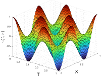
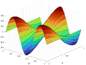
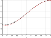
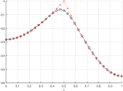
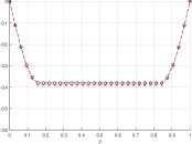
Numerical experiment 2
In this experiment we consider a problem with incomplete information. We take and eliminate one probability variable from the solution by parametrizing for . Hence, we consider the generalized obstacle problem for the transformed solution
| (6.2) |
with the terminal condition ; we take and .
As in the previous experiments we restrict the spatial domain to the interval and approximate (6.2) on a space-time grid with (uniform) mesh sizes , and define the discrete process analogously as in the previous experiment. The approximation in the probability variable is constructed on a uniform mesh with mesh size . We perform the computations using a feedforward neural network (FFN) algorithm 6.3 and a semi-Lagrangian (SL) algorithm 6.4 which employs piecewise linear interpolation in the spatial variable.
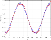
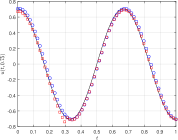
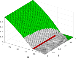
In Figure 6.2 we display the solution computed with at time . To illustrate the effect of the convexity constraint we also display in Figure 6.2 the (nonconvex) solution computed with 6.4 without the convexification step (this corresponds to neglecting the obstacle term in (6.2) and solving the corresponding unconstrained counterpart of (6.2)). In Figure 6.3 we display the two dimensional profiles of the numerical solution crossing the point in the direction of each variable and we observe good agreement between the respective algorithms. In Table 6.2 we display the convergence of the errors decreasing discretization parameters. We observe linear rate of convergence with respect to the discretization in all variables.
Algorithm 6.3 (FFN algorithm - Experiment 2).
For , set and proceed for as follows:
-
For compute:
-
For , set:
-
For , set:
Algorithm 6.4 (SL algorithm - Experiment 2).
For , set and proceed for as follows:
-
For define the map as the piecewise linear interpolant of , i.e., for set
-
For , set:
-
For , set:
| FFN | SL-Scheme | ||||||||
|---|---|---|---|---|---|---|---|---|---|
| MAX-error | rate | RMS-error | rate | MAX-error | rate | RMS-error | rate | ||
| Conv. | 3.13 | 9.63 | – | 6.51 | – | 9.47 | – | 6.05 | – |
| 1.56 | 5.04 | 0.94 | 3.48 | 0.90 | 4.60 | 1.04 | 3.10 | 0.96 | |
| 7.81 | 2.51 | 1.00 | 1.75 | 0.99 | 2.43 | 0.92 | 1.65 | 0.91 | |
| 3.91 | 1.19 | 1.08 | 8.35 | 1.07 | 1.06 | 1.20 | 7.13 | 1.21 | |
| 1.95 | 5.13 | 1.21 | 3.61 | 1.20 | 4.86 | 1.21 | 3.29 | 1.11 | |
| Conv. | 3.13 | 7.77 | – | 4.56 | – | 1.13 | – | 4.59 | – |
| 1.56 | 4.58 | 0.76 | 2.51 | 0.86 | 4.57 | 1.30 | 1.46 | 1.65 | |
| 7.81 | 2.40 | 0.93 | 1.37 | 0.87 | 3.33 | 0.46 | 1.43 | 0.03 | |
| 3.91 | 1.61 | 1.05 | 6.58 | 1.06 | 1.16 | 1.52 | 4.11 | 1.80 | |
| 1.95 | 5.07 | 1.20 | 2.86 | 1.20 | 5.05 | 1.20 | 2.24 | 0.88 | |
| Conv. | 3.13 | 7.35 | – | 5.35 | – | 3.34 | – | 1.84 | – |
| 1.56 | 3.69 | 0.99 | 3.02 | 0.82 | 2.10 | 0.67 | 1.59 | 0.21 | |
| 7.81 | 1.81 | 1.03 | 1.56 | 0.95 | 1.52 | 0.47 | 1.30 | 0.30 | |
| 3.91 | 8.50 | 1.09 | 7.53 | 1.05 | 4.18 | 1.85 | 3.61 | 1.85 | |
| 1.95 | 3.65 | 1.22 | 3.28 | 1.20 | 2.69 | 0.64 | 2.41 | 0.58 | |
Numerical experiment 3
We consider the full problem (1.1) with . As in the previous experiment we eliminate one probability variable from the solution by parametrizing for and consider the following obstacle problem
| (6.3) |
in with a terminal condition , with , . The obstacles are chosen as , with , and , , i.e., the lower obstacle in 6.3 does not depend on . Furthermore, we take , , , . The above problem setup is motivated by the Dynkin game problem (without asymmetric information), considered in [18], which arises in the pricing of Israeli -penalty put options. In this example, asymmetric information arises because the holder of the option does not know exactly how much the writer of the option is going to pay her upon termination of the contract, but she has only knowledge on the a priori probability according to which the additional payment is initially chosen. Our numerical study provides the structure of the game’s state space and depict the equilibrium stopping boundaries, which is of importance for understanding the financial meaning of the equilibrium.
The discretization is performed as in the previous experiment. We restrict the spatial domain to the interval and partition the solution domain uniformly in each variable with the respective mesh sizes , , . In the algorithm below we consider the following Euler approximation of the diffusion process associated with the problem (6.3):
where are i.i.d random variables that take values with equal probability. The computations in this section are performed using the freedforward neural network algorithm 6.5 where we employ a fully connected feedforward neural network that consists of one hidden layer with neurons. We choose , i.e.
as the activation function for the hidden layers and identity function as activation function for the output layer. We use the limited-memory (BFGS) quasi-Newton algorithm [12, 22] to solve the nonlinear least-squares problem at each time-step of the algorithm.
Algorithm 6.5 (FFN - Experiment 3).
For , , we initialize and proceed for as follows:
-
For compute:
-
For , set:
-
For , set:
-
For , set:
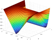
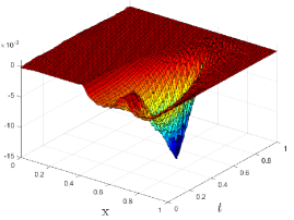
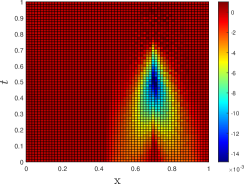
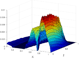
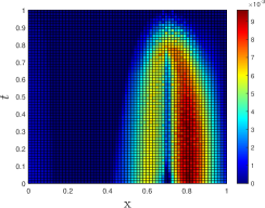
To illustrate the effect of the convexity constraint in 6.3 we compute the solution for of the non-constrained problem
| (6.4) |
In Figure 6.4 we compare the solution of 6.4 to the solution of 6.3. In the top row in Figure 6.4 we plot the difference which takes negative values since is not necessarily convex in the variable, the difference in the bottom row remains positive since is convex in .
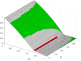
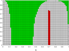
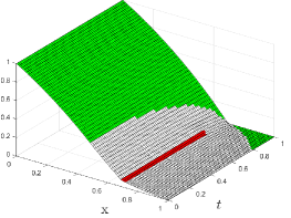
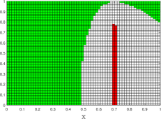
In Figure 6.5 we display space-time graphs of the numerical solution computed with for different values of along with the regions where the two obstacles are active; the red color represents the active region of the lower obstacle and the green color represents the active region of the upper obstacle . In all figures the regions were marked as active if the distance of the numerical solution to the obstacle at the nodes was below a tolerance .

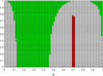
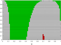
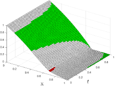

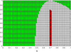
The results in Figure 6.5 show that the writer of the contract would exercise when the price of the underlying stock assumes value . This is consistent with the results in [18]. Also, the buyer would stop when the price of the stock is sufficiently low. This is also consistent to the findings of [18]. Interestingly, we also see from Figure 6.5 that the waiting region (gray area) is not connected, a feature which is not observed in the symmetric information case of [18]. In particular, such a feature of the waiting region does not disappear when or , i.e. in the two symmetric information cases. We repeated the experiment for different combinations of the discretization parameters but the obtained results were qualitatively very similar to those in Figure 6.5. We believe that the presence of a portion of the waiting region for small values of is a numerical artefact, depending on the accuracy of the nonlinear solver used for the neural network approximation. As a matter of fact, the waiting region is observed to be connected (for , i.e. in the symmetric information case) in Figure 6.6, the latter being produced by using a (BR) nonlinear solver or a semi-Lagrangian scheme, for which we have higher accuracy and better convergence. From this example we can thus conclude that sufficient accuracy of the nonlinear solver used for the neural network approximation of free boundaries should be required in order to obtain reliable results.
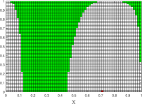
We repeat the simulation with the same discretization parameters as above and employ a feedforward neural network with one hidden layer and neurons (opposed to the neurons used to compute Figure 6.5 above) with the difference that we solve least-squares problem in 6.5 using a Bayesian regularization (BR) algorithm (see [7, 23]). The results displayed in Figure 6.6 for reproduce the expected behavior of the free boundary. For comparison in Figure 6.6 we also display the numerical solution obtained by a semi-Lagrangian algorithm with piecewise linear interpolation (i.e., a modification of 6.5 which employs linear interpolation instead of the least-squares approximation, cf. 6.4) for ; the results are in good qualitative agreement.
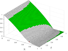
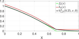
For better illustration we display in Figure 6.7 the graph of the numerical solution for fixed , . We observe that in the numerical solution the lower obstacle is active approximately between and ; and the upper obstacle is active approximately between and .
Acknowledgement
The work of the first and second author was funded by the Deutsche Forschungsgemeinschaft (DFG, German Research Foundation) – Project-ID 317210226 – SFB 1283. The third author was funded by the FWF-Project P346812.
References
- [1] V. Bally and G. Pagès. A quantization algorithm for solving multi-dimensional discrete-time optimal stopping problems. Bernoulli, 9(6):1003–1049, 2003.
- [2] M. Bardi and I. Capuzzo-Dolcetta. Optimal control and viscosity solutions of Hamilton-Jacobi-Bellman equations. Modern Birkhäuser Classics. Birkhäuser Boston, 2009.
- [3] Ľ. Baňas, G. Ferrari, and T. A. Randrianasolo. Numerical approximation of the value of a stochastic differential game with asymmetric information. SIAM J. Control Optim., 59(2):1109–1135, 2021.
- [4] C. M. Bishop. Pattern recognition and machine learning. Information Science and Statistics. Springer, New York, 2006.
- [5] P. Cardaliaguet and C. Rainer. On a continuous-time game with incomplete information. Math. Oper. Res., 34(4):769–794, 2009.
- [6] J. M. Carnicer and W. Dahmen. Convexity preserving interpolation and Powell-Sabin elements. Comput. Aided Geom. Design, 9(4):279–289, 1992.
- [7] F. Dan Foresee and M. Hagan. Gauss-newton approximation to bayesian learning. In Proceedings of International Conference on Neural Networks (ICNN’97), volume 3, pages 1930–1935 vol.3, 1997.
- [8] T. De Angelis, E. Ekström, and K. Glover. Dynkin games with incomplete and asymmetric information. Math. Oper. Res., 47(1):560–586, 2022.
- [9] T. De Angelis, N. Merkulov, and J. Palczewski. On the value of non-Markovian Dynkin games with partial and asymmetric information. Ann. Appl. Probab., 32(3):1774–1813, 2022.
- [10] E. Dynkin. Game variant of a problem on optimal stopping. Soviet Math. Dokl., 10:270–274, 1969.
- [11] F. Gensbittel and C. Grün. Zero-sum stopping games with asymmetric information. Math. Oper. Res., 44(1):277–302, 2019.
- [12] P. E. Gill, W. Murray, M. A. Saunders, and M. H. Wright. A practical anti-cycling procedure for linearly constrained optimization. Math. Programming, 45(3, (Ser. B)):437–474, 1989.
- [13] C. Grün. A probabilistic-numerical approximation for an obstacle problem arising in game theory. Appl. Math. Optim., 66(3):363–385, 2012.
- [14] C. Grün. On Dynkin games with incomplete information. SIAM J. Control Optim., 51(5):4039–4065, 2013.
- [15] K. Hornik, M. Stinchcombe, and H. White. Multilayer feedforward networks are universal approximators. Neural Networks, 2(5):359–366, 1989.
- [16] C. Huré, H. Pham, and X. Warin. Deep backward schemes for high-dimensional nonlinear PDEs. Math. Comp., 89(324):1547–1579, 2020.
- [17] Y. Kifer. Game options. Finance Stoch., 4(4):443–463, 2000.
- [18] C. Kühn and A. E. Kyprianou. Callable puts as composite exotic options. Math. Finance, 17(4):487–502, 2007.
- [19] A. E. Kyprianou. Some calculations for Israeli options. Finance Stoch., 8(1):73–86, 2004.
- [20] R. Laraki. On the regularity of the convexification operator on a compact set. J. Convex Anal., 11(1):209–234, 2004.
- [21] J. Lempa and P. Matomäki. A Dynkin game with asymmetric information. Stochastics, 85(5):763–788, 2013.
- [22] D. C. Liu and J. Nocedal. On the limited memory BFGS method for large scale optimization. Math. Programming, 45(3, (Ser. B)):503–528, 1989.
- [23] D. J. C. MacKay. Bayesian Interpolation. Neural Computation, 4(3):415–447, 05 1992.
- [24] A. M. Oberman and C. W. Craig. The convex envelope is the solution of a nonlinear obstacle problem. Proc. Amer. Math. Soc, 135(6):1689–1694, 2007.
- [25] N. Touzi. Optimal stochastic control, stochastic target problems, and backward SDE, volume 29 of Fields Institute Monographs. Springer, New York; Fields Institute for Research in Mathematical Sciences, Toronto, ON, 2013.
- [26] K. Yosida. Functional Analysis. Grundlehren der mathematischen Wissenschaften. Springer Berlin Heidelberg, 2013.