Moduli Space of Dihedral Spherical Surfaces and Measured Foliations

Abstract

Cone spherical surfaces are Riemannian surfaces with constant curvature one and a finite number of conical singularities. Dihedral surfaces, a subset of these spherical surfaces, possess monodromy groups that preserve a pair of antipodal points on the unit two-sphere within three-dimensional Euclidean space. On each dihedral surface, we naturally define a pair of transverse measured foliations, which, conversely, fully characterize the original dihedral surface. Additionally, we introduce several geometric decompositions and deformations for dihedral surfaces. As a practical application, we determine the dimension of the moduli space for dihedral surfaces with prescribed cone angles and topological types. This dimension serves as a measure of the independent geometric parameters determining the isometric classes of such surfaces.

2020 Mathematics Subject Classification]32G15, 30F30, 53A10

1 Introduction

The investigation into conformal constant curvature metrics with conical singularities on Riemann surfaces represents a natural extension of uniformization theory. Given a compact Riemann surface $\ignorespaces X$ of genus $\ignorespaces g$ with $\ignorespaces n$ distinct points $\ignorespaces P:=\{p_{1},\ldots,p_{n}\}$ and an angle vector $\ignorespaces\vec{\theta}:=(\theta_{1},\ldots,\theta_{n})\in\mathbb{R}_{+}^{n}$ where $\ignorespaces\theta_{i}\neq 1$ , a central question arises: the existence of a singular conformal metric $\ignorespaces g$ of constant curvature $\ignorespaces K\in\{-1,0,+1\}$ with a conical singularity of angle $\ignorespaces 2\pi\theta_{i}$ at $\ignorespaces p_{i}$ . Expressed in complex coordinates, this quest implies the existence of a local chart $\ignorespaces z$ , where $\ignorespaces g$ can be written as

$$\mathrm{d}s=\frac{2\alpha\lvert z\rvert^{\alpha-1}\lvert\mathrm{d}z\rvert}{1+K\lvert z\rvert^{2}},$$

with $\ignorespaces\alpha=\theta_{i}$ at $\ignorespaces p_{i}$ and $\ignorespaces\alpha=1$ outside $\ignorespaces P$ . This line of inquiry has historical roots tracing back to the works of Picard and Poincaré Poi (98); Pic (05). A surface equipped with such a metric and constant curvature is referred to as a cone hyperbolic, flat, or spherical surface.

The Gauss-Bonnet Formula provides a necessary condition for the existence of such metrics, stipulating that $\ignorespaces 2-2g+\sum_{i=1}^{n}(\theta_{i}-1)$ should share the same signature as $\ignorespaces K$ . For $\ignorespaces K=-1,0$ , this condition is also sufficient, and the metric is unique Hei (62); McO (88); Tro (91). However, in the case of $\ignorespaces K=+1$ , the problem remains wide open, with only partial results available, as found in Tro (89, 91); LT (92); UY (00); Ere (04); LW (10); BDMM (11); EGT (14); EG (15); Ere20b ; LSX (21); dBP (22). A comprehensive survey Ere (21) detailing the story and progress is also recommended. Neglecting the underlying complex structures of cone spherical surfaces, we are aware of the constraint on their cone angles. For $\ignorespaces g>0$ , the Gauss-Bonnet condition is also sufficient MP (19). When $\ignorespaces g=0$ , in addition to the Gauss-Bonnet condition, the complete angle constraint involves additional profound conditions, detailed in MP (16); Li (19); Ere20a .

Partial results on the moduli space of spherical surfaces also exist. For example, small deformations of such surfaces are studied in MZ (20, 22). Local properties of the Teichmüller space with small prescribed cone angles, using geometric analysis and elliptic operators, are examined in MW (17). A walls-and-chambers structure of the moduli space with a fixed topological type and variable cone angles is obtained in Tah (22), through a geometric decomposition of spherical surfaces. Results on spherical tori with a single conical singularity are particularly rich. These surfaces can be studied using elliptic functions and modular forms LW (10); CLW (15); CKL (17); LW (17). The moduli space with different prescribed angles is explicitly described in EMP (20) through a geometric approach.

There is a special class of cone spherical surfaces with special monodromy, called dihedral surfaces (Definition 2.2), which we better understand. They are further divided into two subclasses, known as co-axial and strict dihedral surfaces. These surfaces are closely associated with meromorphic abelian and quadratic differentials on the underlying Riemann surfaces, with real periods, as discovered by CWWX (15); SCLX (20). The sufficient and necessary conditions on the cone angles for these surfaces have been completely obtained in GT (23). This paper continue the study of dihedral surfaces and their moduli space, focusing on the geometric aspect. Let $\mathcal{M}sph^{C}_{g,n}(\vec{\theta})$ and $\mathcal{M}sph^{D}_{g,n}(\vec{\theta})$ denote the moduli space of co-axial and strict dihedral surfaces with a fixed genus and prescribed cone angles (Definition 3.4). Each dihedral surface induces a pair of transverse measured foliation $(F,G)$ (Subsection 3.2), which provides a crucial decomposition of the surface, leading to a geometric coordinate for the moduli space. Then we compute the maximum number of independent parameters that determine isometric classes of such surfaces, which corresponds to the dimension of the moduli space (Theorem 5.10, 5.14).

Theorem 1.1.

Given an angle vector $\vec{\theta}=(\theta_{1},\cdots,\theta_{n})\in\mathbb{R}^{n}_{+}$ with $\theta_{i}\neq 1$, and $2g-2+n>0$. Assume that all the moduli spaces as follows are non-empty.

1. The maximal real dimension of $\mathcal{M}sph^{D}_{g,n}(\vec{\theta})$ is $2M_{E}+M_{O}+2g-2$, where $M_{E}$ is the number of integers in $\vec{\theta}$, $M_{O}$ is the maximal even number not exceeding the number of half-integers in $\vec{\theta}$.

2. The real dimension of $\mathcal{M}sph^{C}_{g,n}(\vec{\theta})$ is $2M_{E}+2g-1$ if $(g,n-M_{E})\neq(0,0)$, where $M_{E}$ is the number of integers in $\vec{\theta}$. And the real dimension of $\mathcal{M}sph^{C}_{0,n}(\vec{\theta})$ is $2n-3$ when $g=0,M_{E}=n$.

The constraints on the cone angle vector such that all the above moduli spaces are non-empty are quite complicated, whose full list for various cases could be found in Gendron-Tahar’s work GT (23). For most settings of $(g,n)$, the only constrain on the angle vector is the strengthened Gauss-Bonnet inequality (GT, 23, Theorem 1.2).

The term “maximal dimension” suggests that the moduli space may have disjoint components of different dimensions (see Example 5.16). This leads to a refined moduli space by prescribing the topological type of the foliation $(F,G)$ (see Definiton 3.7, 3.8). This is equivalent to restricting to a certain stratum of the differentials. In fact we count the dimension of such refined moduli spaces (Theorem 5.8, 5.13).

Remark. Studying the entire moduli space $\mathcal{M}sph_{g,n}(\vec{\theta})$ is a much more challenging problem, which currently seems to be beyond our reach. It is claimed in (MP, 19, Section 6) that when $\vec{\theta}$ satisfies a so-called ”non-bubbling condition”, the real dimension of the moduli space of spherical surfaces with genus $g$ and $n$ cone angles prescribed equals $6g-6+2n$. However, this non-bubbling condition seems to be irrelevant to the angle constraint for dihedral surfaces. On one hand, the angle vector for a co-axial surface never satisfy non-bubbling condition. However, there do exist strict dihedral surfaces whose angle vectors satisfy the non-bubbling condition.

Here is our strategy for proving the main theorem, using the strict dihedral case as an example. A dihedral surface together with a pair of foliations is called a foliated surface (Definition 3.2). Our first step is counting the dimension of the moduli space of foliated surfaces, with a prescribed angle vector and topological type of the foliations (Definition 3.7 and Theorem 5.8). This involves studying the strip decomposition of a foliated surface (Definition 4.4) and the concept of generic surfaces (Definition 4.17). The dimension of this subset is determined using the connection matrix (Definition 5.4), which captures the linear constraints on the geometric parameters of a strip decomposition. Next, we apply the identification lemma (Subsection 5.1) to pass this result to a subset of the original moduli space, by forgetting the foliation structure. The identification lemma shows that the choice of strip decomposition for a given strict dihedral surface is always finite (Proposition 5.2). Finally, by combining our findings with the results of Gendron-Tahar in GT (23), we obtain the maximum dimension of moduli spaces among all possible topological types.

The overall outline of our approach is summarized in the diagram below. The co-axial case follows a similar proof strategy, with some technical modifications.

The paper is organized as follows.

• Section 2 provides perliminaries on cone spherical surfaces, abelian and quadratic differentials and measured foliations. We also recall the definitions of co-axial and dihedral metrics.

• Section 3 introduces the main character, the longitude and latitude foliation on dihedral surfaces. Various moduli spaces are defined, preparing for the final dimension count.

• Section 4 presents two mutually “prependicular” geometric decompositions of dihedral surfaces based on the above two foliation structures. Several geometric deformations are given, which could be thought of analogues of periodic coordinates for translation surfaces.

• Section 5 is dedicated to dimension counting. We define and study the connection matrix, and proof the identification lemma. The dimension counting for various moduli spaces is then carried out sequentially.

Acknowledgements. Both authors would like to express their heartfelt gratitude to Guillaume Tahar for his excellent series of talks during his visit to USCT in August 2023. The ideas of decomposition and sliding were greatly inspired by the insightful discussions with Guillaume. The authors would also like to thank Jijian Song for engaging conversations on this topic. B.X. is supported in part by the Project of Stable Support for Youth Team in Basic Research Field, CAS (Grant No. YSBR-001) and NSFC (Grant Nos. 12271495, 11971450, and 12071449).

2 Preliminaries

In this paper, we are not fixing the underlying Riemann surface structure. So a compact “surface” will refer to both a topological surface (possibly with metric) and a Riemann surface, according to the context. And we prefer “cone spherical surfaces” to “cone spherical metrics”.

2.1 Cone spherical surfaces

We are considering Riemannian metric of constant curvature $K\in\{-1,0,+1\}$ on a compact surface with conical singularities. This means that for every point, in the geodesic polar coordinates, the metric is locally expressed as

$$\mathrm{d}s^{2}=\left\{\begin{array}[]{lll}\mathrm{d}r^{2}+\alpha^{2}\sinh^{2}r\mathrm{d}\theta^{2}&,K=-1&\quad\text{(hyperbolic geometry)}\\ \mathrm{d}r^{2}+\alpha^{2}r^{2}\mathrm{d}\theta^{2}&,K=0&\quad\text{(flat geometry)}\\ \mathrm{d}r^{2}+\alpha^{2}\sin^{2}r\mathrm{d}\theta^{2}&,K=+1&\quad\text{(spherical geometry)}\\ \end{array}\right.$$

with the cone angle of that point being $2\pi\alpha>0$. Here $\alpha\neq 1$ only at finitely many isolated points, called cone points. We focus on the case of $K=+1$ in this paper. A surface equipped with such a metric is called cone spherical surface.

There is also a geometric description. Recall some notations of MP (16). Let $\mathbb{S}^{2}\subset\mathbb{R}^{3}$ be the unit sphere, parameterized by spherical coordinates

$$\mathbb{S}^{2}=\big{\{}\ (\psi,\phi):=(\cos\psi\sin\phi,\sin\psi\sin\phi,\cos\phi)\ \big{\rvert}\ \psi\in[0,2\pi),\ \phi\in[0,\pi]\ \big{\}}$$

and $N=(0,0),S=(0,\pi)$ be the north and south pole. Given $\alpha\in(0,1)$ and $r\in(0,\pi]$,

$${\color[rgb]{0,0,0}B_{\alpha}(r)}:=\big{\{}\ (\psi,\phi)\ \rvert\ \psi\in[0,2\pi\alpha],\ \phi\in[0,r)\ \big{\}}$$

is called a sector of angle $2\pi\alpha$ centered at $N$ with radius $r$. Let $P=(0,r),Q=(2\pi\alpha,r)$ be the other two vertices, and $NP,NQ$ be the two geodesic boundary radii of the sector.

For any $\theta>0$, let $M$ be the smallest positive integer such that $\theta/M<1$. We take $M$ copies of $B_{\theta/M}(r)$, denoted by $B^{(i)}$ with vertices $N^{(i)},P^{(i)},Q^{(i)}$, $i=1,\cdots,M$. Now gluing the pair of radii $N^{(i-1)}Q^{(i-1)}$ and $N^{(i)}P^{(i)}$ by the $\phi$ parameter for each $i={\color[rgb]{0,0,0}2},\cdots,M$, we obtain a topological sector denoted by $B_{\theta}(r)$, and obviously generalizing the previous one. This serves as a local model for cone vertices of polygons. See figure 1.

If the remained two boundary radii $N^{(M)}Q^{(M)},N^{(1)}P^{(1)}$ is further glued, we obtain a cone of angle $2\pi\theta$ with radius $r$, denoted by $S_{\theta}(r)$. This serves as a local model for cone points on surfaces. In both $B_{\theta}(r)$ and $S_{\theta}(r)$, the unique image of all $N^{(i)}$’s is the cone point. Note that every point on $\mathbb{S}^{2}$ has a neighborhood isometric to $S_{1}(r)$ for some small $r$. Then we can consider a cone spherical surface as a metric compact surface such that every point has a neighborhood isometric to some $S_{\theta}(r)$, with $\theta=\theta_{i}$ at $p_{i}$ and $\theta=1$ outside $P$. This natually induce a complex structure on the surface.

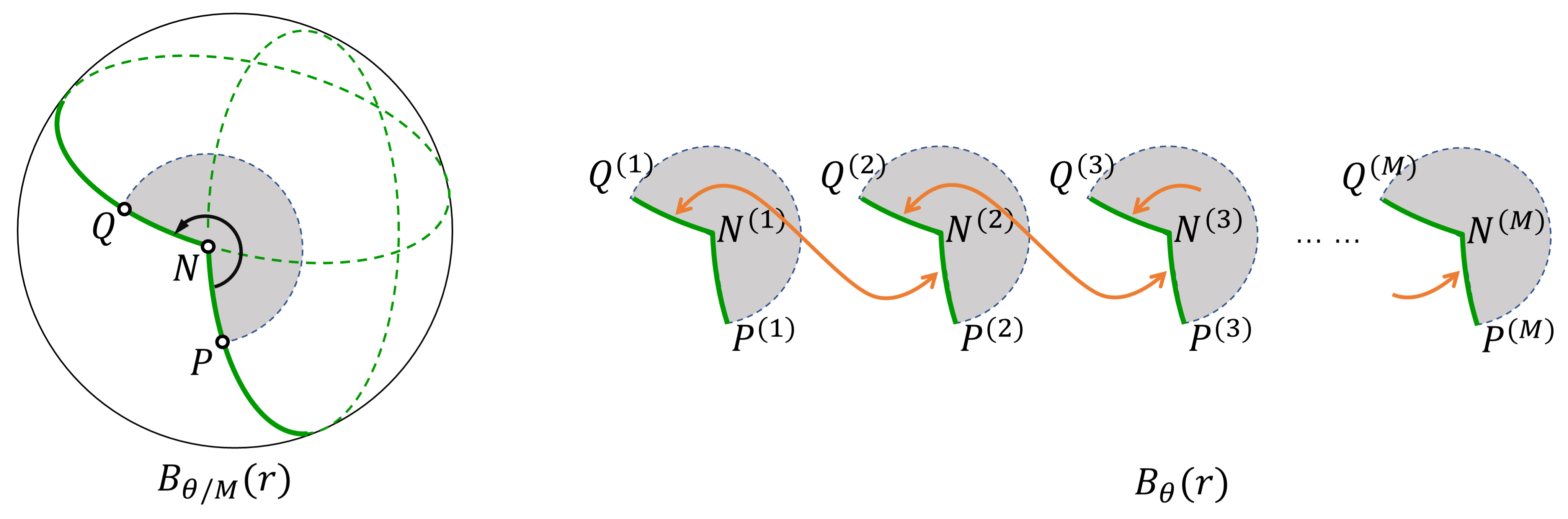
Figure 1: Gluing sectors of small angle to obtain a local model for cone vertex.

When $r=\pi$, the closure ${\color[rgb]{0,0,0}B_{\theta}}:=\overline{B_{\theta}(\pi)}$ is called a spherical bigon of angle $2\pi\theta$, or a bigon of width $\theta$ (see Section 3.2). It is bounded by two geodesic segments of length $\pi$, homeomorphic to a closed disk. It is foliated by a continuous family of disjoint geodesic arcs of length $\pi$ connecting the two cone points. So it is also called a foliated singular sphere in Tah (22). ${\color[rgb]{0,0,0}S_{\theta}}:=\overline{S_{\theta}(\pi)}$ is called a football of angle $2\pi\theta$. It is a topological sphere with two cone points of the same angle.

2.2 Developing map, monodromy and dihedral surface

We will frequently switch between the unit sphere $\mathbb{S}^{2}$ and the Riemann sphere $\mathbb{C}\cup\{\infty\}$. The isometry group $\mathrm{SO}(3,\mathbb{R})$ of the unit sphere is identified with

$$\mathrm{PSU}(2)=\left\{\ z\mapsto\frac{az+b}{-\bar{b}z+\bar{a}}\ \bigg{\rvert}\ a,b\in\mathbb{C},\left\lvert a\right\rvert^{2}+\left\lvert b\right\rvert^{2}=1\ \right\}\subset\mathrm{PGL}(2,\mathbb{C})$$

acting on the Riemann sphere. And the standard spherical metric on the Riemann sphere is $g_{sph}=4\lvert\mathrm{d}w\rvert^{2}/(1+\lvert w\rvert^{2})^{2}$

Given a cone spherical surface $\Sigma$, its metric natually induces a complex structure on it. There exists a multivalued meromorphic function $D$ on $\Sigma$, branched at the cone points $P$. Futhermore, the pullback metric $D^{*}(g_{sph})$ of $g_{sph}$ coincidents with the cone spherical metric on $\Sigma$. Such map $D$ is called a developing map. It has monodromy in $\mathrm{PSU}(2)$. That is, given a point $z$ and a closed curve $\gamma$ in $\Sigma-P$, and let $D(\gamma\cdot z)$ be the analytic continuation of $D$ along $\gamma$, then there exists some $\rho(\gamma)\in\mathrm{PSU}(2)$ such that $D(\gamma\cdot z)=\rho(\gamma)\big{(}D(z)\big{)}$. The element $\rho(\gamma)$ depends only on the homotopy class of $\gamma$. Thus a developing map $D$ induces a monodromy representation $\rho_{D}:\pi_{1}(\Sigma-P)\to\mathrm{PSU}(2)$ and its image is called monodromy group. The developing map is unique up to a $\mathrm{PSU}(2)$ post-composition, and the monodromy representation and group is also unique up to a $\mathrm{PSU}(2)$ conjugation. It is a local isometry outside the cone points, and can be regarded as an infinite covering of unit disk branched at the origin around each cone point. See UY (00); CWWX (15); SCLX (20) for more details.

The developing map can be defined geometrically as well, using the concept of $(G,X)$-manifolds, but small modification for cone points is needed. Here $X=\mathbb{S}^{2}$ and $G=\mathrm{SO}(3,\mathbb{R})$. We refer to (Thu, 97, Chapter 3) for such exposition.

Usually the monodromy group of a cone spherical surface is very complicated. However, there are special classes of surfaces with simpler monodromy. These surfaces are of great interest, having a strong relation with meromorphic differentials and foliations on Riemann surface, and will be our main object. We shall denote the monodromy group by $\rho(\pi_{1})$ for convenience.

Definition 2.1.

A cone spherical surface is called co-axial if its monodromy group fixes an axis of the sphere. Equivalently, $\rho(\pi_{1})$ is conjugated to a subgroup of

$$\mathrm{U}(1):=\left\{\ z\mapsto\mathrm{e}^{\mathbf{i}\theta}z=\frac{\mathrm{e}^{\mathbf{i}\theta/2}z}{\mathrm{e}^{-\mathbf{i}\theta/2}}\ \bigg{\rvert}\ \theta\in\mathbb{R}\ \right\}\cong\mathrm{SO}(2,\mathbb{R}).$$

This is equivalent to the reducible metric by Umehara and Yamada UY (00).

This monodromy condition is slightly generalized in SCLX (20); GT (23).

Definition 2.2.

A cone spherical surface is called dihedral if its monodromy group preserves a pair of antipodal points of the sphere. Equivalently, $\rho(\pi_{1})$ is conjugated to a subgroup of

$$\mathrm{O}(2):=\left\{\ z\mapsto\mathrm{e}^{\mathbf{i}\theta}z,\ z\mapsto\frac{\mathrm{e}^{\mathbf{i}\theta}}{z}\ \bigg{\rvert}\ \theta\in\mathbb{R}\ \right\}\cong\mathbb{Z}_{2}\ltimes\mathrm{U}(1).$$

A non-co-axial dihedral surface is called strict dihedral.

2.3 Differentials and dihedral surfaces

Let $X$ be a compact Riemann surface of genus $g\geqslant 0$ and $K_{X}$ its canonical line bundle. An abelian differential $\omega$ is a meromorphic 1-form on $X$. A quadratic differential $q$ is a meromorphic section of $K_{X}^{\otimes 2}$. Its critical points are the zeros and poles of the differential. In a coordinate chart, the differential is expressed as $\omega(z)\mathrm{d}z$ or $q(z)\mathrm{d}z^{2}$, where $\omega(z)$ and $q(z)$ are meromorphic functions, compatible with coordinate transformation. Here we only consider abelian differentials with at worst simple poles, and quadratic differentials with at worst double poles. Locally, in a simply connected neighborhood of a non-critical point, a quadratic differential $q$ is a square of an abelian differential, but globally it is not the case in general. We call a quadratic differential primitive if it is not globally the square of an abelian differential.

Such a differential defines a conformal cone flat metric on $X$. Outside the critical points, one can always choice suitable coordinates such that the differential is simply expressed as $\mathrm{d}z$ or $\mathrm{d}z^{2}$. The metric near a simple pole of an abelian differential or a double pole of a quadratic differential forms a half-infinite cylinder. All other crtitical points become cone points of angle $k\pi(k\in\mathbb{N}_{+})$ in that metric. We refer to Str (84); Hub (06) for more details.

Now suppose $\Sigma$ is a dihedral surface, with a developing map $D$. By post-composing a $\mathrm{PSU}(2)$ element we may assume that its monodromy group preserves $0,\infty$. Then one checks that $D^{*}\left(\mathrm{d}z^{2}/z^{2}\right)$ is a well-defined quadratic differential on $X$, beacause $\mathrm{d}z^{2}/z^{2}$ is invariant under $\mathrm{O}(2)$ transformations on the Riemann sphere. For co-axial surfaces, one obtains an abelian differential by pulling back the 1-form $\mathrm{d}z/z$. This observation provides an linkage betweeen cone spherical surfaces, quadratic differentials and cone flat surfaces, which is crucial to this present work. The next part and next section provides a geometric topology version of it.

For more details on dihedral surfaces and differentials, or complex analytical aspect of this relation, see CWWX (15); SCLX (20); GT (23).

2.4 Measured foliations

The topological information of an abelian or quadratic differential is carried by a pair of transverse measured foliations induced by it. For simplicity and our purpose, we stick to compact surface without boudary in this paper. We refer to (FLPe, 91, Exposé 5) or (PT, 07, Section 2) for more facts about topological measured foliations, and (Hub, 06, Chapter 5) for well-described relations between differntials, foliations and flat geometry.

A (singular) foliation on a surface is a decomposition of the 2-dimensional surface into 1-dimensional submanifolds, except for finite isolated points which are called singularities. Equivalently, in the smooth category, it is a line field with isolated singular set. The 1-dimensional submanifolds, or the trajectories of the line field, are called leaves. The singularities are the points where multiple leaves meet. Leaves staring from a singularity are called singular leaves. Leaves without a singularity are called regular leaves.

Each singularity is a $s$-prong, where $s$ is the number of the leaf segments meeting at the point. Here we shall only consider $s\geqslant 0$. See Figure 2 for a local picture when $s=0,1,2,3$. In particular, a $2$-prong singularity is actually regular. The index of an $s$-prong singularity $p$ is defined to be ${\color[rgb]{0,0,0}\mathrm{Ind}(p)}:=2-s.$ Overall, this is a variation of the index for a zero of a vector field.

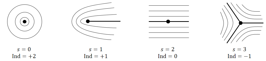
Figure 2: Examples of singularities with various indexes.

The indexes of singularities reflect global surface topology. We have the following index formula, induced from the Poincaré-Hopf theorem for vector fields. This can be regarded as a topological version of Gauss-Bonnet theorem.

Theorem 2.3 (Poincaré-Hopf Theorem).

Suppose $F$ is a foliaiton on a closed surface $S$ of genus $g\geqslant 0$. Then

$$\sum_{\mathrm{singularity}\ p}\mathrm{Ind}(p)=2(2-2g).$$ (2.1)

A measured foliation on closed surface $S$ is a foliation equipped with a positive measure on each transverse arc, which is equivalent to the Lebesgue measure on a closed interval of $\mathbb{R}$. These measures are invariant by isotopies of the transverse arcs during which each point stays on the same leaf.

Usually we consider the equivalence classes of measured foliations differed by two kinds of transformations. Homeomorphisms of the surface which are isotopic to the identity will send one foliation to the other and preserving the transverse measures. Another one are Whitehead moves. These are deformations of the surface that take place in a neighborhood of arcs that join two singular points and whose effect is to collapse such an arc to a point. However, in our case, every singular point will be a cone point. So Whitehead move is not allowed in finite time because it merge cone points.

Each quadratic differential $q$ on a Riemann surface $X$ induces a pair of transverse measured foliations $(H_{q},V_{q})$. This means the singularities of $H_{q},V_{q}$ are the same, with the equal indexes, and leaves of $H_{q}$ and $V_{q}$ intersect transversely outside the singularities. These measured foliations are induced by the trajectories of the differential.

We only include a heuristic example here, because no serious complex analysis aspect of differentials is used later. Full exposition can be found in mentioned references. Cases for abelian differentials are similar.

Consider the quadratic differential $\mathrm{d}z^{2}$ on $\mathbb{C}$. A horizontal trajectory of $q$ is a horizontal line with constant $y$ coordinate. All horizontal trajectories form the horizontal foliation $H_{q}$. Its transverse measure on a transverse arc is given by the total variation of $y$ coordinated. Namely it is given by $\left\lvert\mathrm{d}y\right\rvert=\left\lvert\mathrm{Im}\sqrt{q}\right\rvert$. The vertical foliation $V_{q}$ is defined similarly, by replacing all $y$ coordinate with $x$ coordinate. For a quadratic differential on a general Riemann surface, one just need to find some suitable local coordinates outside the singularities and biholomorphically map open subset on $X$ to open subset on $\mathbb{C}$. For a singularity $p$ of $q$, one can choose local charts such that $q=z^{k}\mathrm{d}z^{2}$ where $k=-\mathrm{Ind}(p)$. Then $p$ is a $(2-k)$ prong of both foliation.

Note that around a double pole, all horizontal trajectories converge to the pole, while all vertical trajectories are closed cycles winding around the pole. We define both cases to be a singularity of the foliation with index $+2$.

3 The latitude and longitude foliation

Now we shall consider a class of measured foliations slightly adjusted from the one directly induced by differentials. These foliations provide more geometric informations, thus highly helpful in the study of dihedral cone spherical surfaces.

3.1 On the unit sphere

Definition 3.1.

There is a natural pair of transverse foliations on the 2-sphere.

• The latitude foliation $\mathcal{F}_{L}$ consists of all latitude circles on $\mathbb{S}^{2}$. Its measure of a transverse arc is given by the total variation of latitude.

• The longitude foliation $\mathcal{G}_{L}$ consists of all meridian lines on $\mathbb{S}^{2}$. Its measure of a transverse arc is given by the total variation of longitude.

All leaves are lines with constant $\psi$ or $\phi$ coordinate. Leaves of $\mathcal{F}_{L}$ are also the level sets of Morse function $z=\cos\phi$ on $\mathbb{S}^{2}$. The equator is the only geodesic leaf of $\mathcal{F}_{L}$. Leaves of $\mathcal{G}_{L}$ are geodesics of length $\pi$ connecting two poles. The poles $N,S$ are the only singularities of both foliation, with index $+2$.

Consider the conformal Mercator map $Mer:\mathbb{C}\to\mathbb{S}^{2}-\{N,S\}$ given by

$$Z=\psi+\mathbf{i}Y\longmapsto\left(\psi,2\arctan(\mathrm{e}^{Y})\right).$$ (3.1)

This is the conformal universal cover of the twice punctured sphere. Then $\mathcal{G}_{L}$ is exactly the pulled-back of vertical measured foliation $\mathrm{d}\psi$. $\mathcal{F}_{L}$ is the pulled-back of horizontal foliation with a different measure given by $\mathrm{d}Y/\cosh Y$. If we use the coordinate $z=r\mathrm{e}^{\mathbf{i}\theta}$ of the Riemann sphere, $Mer:\mathbb{C}\to\mathbb{C}^{*}$ is given by

$$Z=\psi+\mathbf{i}Y\longmapsto\exp(\mathbf{i}Z)=\mathrm{e}^{-Y}\mathrm{e}^{\mathbf{i}\psi}.$$ (3.2)

Then $\mathcal{G}_{L}$ is given by $\mathrm{d}\theta$ and $\mathcal{F}_{L}$ is given by $2\mathrm{d}r/(1+r^{2})$. So $(\mathcal{F}_{L},\mathcal{G}_{L})$ is topologically equivalent to the pair of measured foliations induced by abelian differential $\mathbf{i}\mathrm{d}z/z$ on the Riemann sphere (or simply $\mathrm{d}Z$ on the covering $\mathbb{C}$), with a modified measure. We are using the measure to record spherical geometric quantities. This pair of measured foliations in the coordinate of the Riemann sphere is also denoted by $(\mathcal{F}_{L},\mathcal{G}_{L})$.

3.2 On dihedral surfaces

Given a dihedral cone spherical surface $\Sigma$ with a developing map $D$, by post-composing a $\mathrm{PSU}(2)$ element we may assume that its monodromy group preserves $0,\infty$. It is easy to checks that $\mathrm{d}\theta$ and $2\mathrm{d}r/(1+r^{2})$ is fixed by $\mathrm{U}(1)$-action, and is invariant up to signature under $\mathrm{O}(2)$-action. So as measured foliations, $\mathcal{F}_{L},\mathcal{G}_{L}$ are fixed by $\mathrm{O}(2)$-action.

Definition 3.2.

Let $\Sigma$ be a dihedral cone spherical surface with a developing map $D$ such that $\rho(\pi_{1})$ preserves $0,\infty$.

1. ${\color[rgb]{0,0,0}F}:=D^{*}(\mathcal{F}_{L})$ and ${\color[rgb]{0,0,0}G}:=D^{*}(\mathcal{G}_{L})$ are well-defined measured foliations on $\Sigma$. $F$ and $G$ are also called latitude and longitude foliation of $\Sigma$ with respect to $D$, regarded as horizontal and vertical foliation.

2. A foliated dihedral surface is a dihedral surface $\Sigma$ together with a pair of latitude and longitude foliation $(F,G)$ induced by some developing map. It is denoted by a triple $(\Sigma\mathchar 24635\relax\;F,G)$.

Note that the function $\left\lvert\cos\phi\right\rvert$ is $\mathrm{O}(2)$-invariant on $\mathbb{S}^{2}$. So for any dihedral surface $\Sigma$ with $D$ as above, $\left\lvert\cos\phi\right\rvert$ can be pulled back to a function $H$ by the developing map. $H:\Sigma\to[0,1]$ is called the absolute latitude function. The latitude foliation $F$ consists of the level sets of $H$.

Remarks.

(1). $\cos\phi$ itself is $\mathrm{U}(1)$-invariant. So for co-axial surfaces, it can be pulled back to a Morse function $h$ on $\Sigma$ by the developing map $D$. This is similar to the function $\Phi$ in CWWX (15); WWX (22) and we have $2h+2=\Phi$.

(2). A meromorphic quadratic differential induces a dihedral cone spherical metric if and only if the integral of $\sqrt{q}$ is real along any closed curve and any choice of analytic branch of square root Li (19); SCLX (20). One can check that “being real” is well-defined. Note that the horizontal and vertical direction here is inverse to the usual one defined for the pulling-back differentials of $\mathrm{d}z/z$.

Strebel differentials, whose regular horizontal leaves are all simple closed curves around exactly one pole, form a special class of such differentials. They correspond to hemispherical surfaces in (GT, 23, Section 2.5), and are related to limit surfaces of grafting along a multicurve (Gup, 14, Section 5.2).

(3). There may be different choices of $(F,G)$ on a given $\Sigma$. See Example 4.6. Studying the moduli space of foliated surface is the actual goal, and the possibility of different choices is studied in Section 5.

3.3 Local information of singularities

Let $(\Sigma\mathchar 24635\relax\;F,G)$ be a foliated dihedral surface from a developing map $D$, and $N,S$ be the north and south pole of the sphere.

Definition 3.3.

1. The preimage of the equator $\{\phi=\frac{\pi}{2}\}\subset\mathbb{S}^{2}$ of $D$ is called the equatorial net of the foliated surface (or both foliations $F,G$), denoted by $\mathcal{E}$.

2. The preimages of poles $\{N,S\}$ of $D$ are called the poles of both foliations, denoted by ${\color[rgb]{0,0,0}Q}:=D^{-1}\{N,S\}$. They are singularities with index $+2$.

3. All the other singularities are called zeroes of both foliations, with index $\leqslant+1$.

Equivalently, using the absolute latitude function $H$ defined previously, we have $\mathcal{E}=H^{-1}(0)$, $Q=H^{-1}(1)$.

Unlike the case of flat surface, the equatorial net is the only geodesic leaves of $F$. This makes the leaves of $F$ geometrically unequal while they can be topologically equivalent. The only set of geodesic leaves of $F$ is the equatorial net $\mathcal{E}$. Whenever $\mathcal{E}$ is disjoint from the cone point set $P$, it is a finite union of smooth simple closed geodesics on $\Sigma$. If $\mathcal{E}\cap P$ is non-empty, it still consists of finitely many closed geodesics, intersecting at several cone points.

Let $P\subset\Sigma$ be the finite set of all cone points and $p\in P$ be a cone point of angle $2\pi\theta$, Every cone point must be a singularity, but a singularity of the foliations may be a smooth point. By the geometry of $\mathrm{O}(2)$ action, the position of cone points restricts its cone angles. If $p$ lies on the equatorial net, then the monodromy representation of a close loop surrounding it keeps the equator, hence be a power of $\pi$-rotation about its developing map image. If $p$ is a preimage of the poles, then the representation of a close loop can be arbitrary rotation about it. Finally, if $p$ does not lie on the equator or the preimage of poles, the representation of a close loop must be trivial and the cone angle is a integer multiple of $2\pi$.

We summarize local information of singularities of $F$ in the following table.

singularity $x$ of $F$	$\in P\cap Q$	$\in P\cap\mathcal{E}$	$\in P-(\mathcal{E}\cup Q)$	$\in Q-P$
cone angle	arbitrary	$k\pi$	$2k\pi$	(smooth point)
index	$+2$	$2-k$	$2-2k$	$+2$

Table 1: Local information from singularities of $F$, for dihedral surfaces. Recall that $P$ is the set of all cone points; $Q$ is the set of pole singularities; and $\mathcal{E}$ is the equatorial net.

For co-axial surface, whenever $p\in P-Q$, its cone angle must be integer multiple of $2\pi$, since $\pi$-rotation about a point on the equator is not allowed.

To sum up, for dihedral surfaces, the poles of $F$ provide geometric information, while the zeros of $F$ provide more topological information. The pair of measured foliations $(F,G)$ completely determines a dihedral cone spherical surface.

3.4 More about the measure

There is a little difference between the measure used here and the usual measure for flat surface induced by foliations or differentials: most leaves are not a geodesic here, so the measure records the geometry in particular directions.

The total measure of leaf segments in $F,G$ is most concerned. We give a brief description next. The ideas are exactly the same as the general theory of measured foliation.

Let $\gamma:[0,1]\to\Sigma$ be an embedded leaf segment of $G$ without singularity in its interior. Then $\gamma$ is a geodesic arc. The total measure of $\gamma$ under $F$, or the intersection number of $F$ and $\gamma$, is defined to be its spherical length and denoted by $i(F,\gamma)$.

When $\gamma=\gamma_{1}\cup\cdots\cup\gamma_{n}$ is a finite union of piecewisely embedded leaf segments, and singularities appear only at endpoints of each segment, then $i(F,\gamma):=\sum i(F,\gamma_{i})$.

Let $\delta:[0,1]\to\Sigma$ be an embedded leaf segment of $F$ without singularity in its interior. Pick an analytic branch of the developing map $D$ such that it is well-defined along $\delta$. Then its total measure under $G$, or the intersection number $i(G,\delta)$, is defined to be the total longitude variation of $D({\delta})$. The case where $\delta$ is a finite union of embedded leaf segments is similar as above.

Equivalently, we can consider the equatorial projection

$$\mathrm{pr}:\mathbb{S}^{2}-\{N,S\}\longrightarrow\{\phi=\frac{\pi}{2}\}\subset\mathbb{S}^{2},\quad(\psi,\phi)\mapsto(\psi,\pi/2)=(\cos\psi,\sin\psi,0).$$

Then $i(G,\delta)$ equals to the spherical length of $\mathrm{pr}\circ\delta$ as a curve. In particular, when $\delta$ is a closed leaf surrounding a pole $q$ of the foliation, $i(G,\delta)$ equals to the cone angle $2\pi\theta_{i}$ if $q=p_{i}\in P$, and equals to $2\pi$ if $q\notin P$. This is the same as the residue of differential at a double pole, multiplied by $2\pi$.

3.5 Various moduli spaces

Now we are ready to state several kinds of moduli spaces used for the dimension count. As before, let $\vec{\theta}:=(\theta_{1},\cdots,\theta_{n})\in\mathbb{R}_{+}^{N}$ be an angle vector with $\theta_{i}\neq 1$.

Definition 3.4.

1. A labeled surface is a cone spherical surface whose cone points are labeled as $p_{1},\cdots,p_{n}$ such that the cone angle of $p_{i}$ is $2\pi\theta_{i}$, $i=1,\cdots,n$.

2. Let $\Sigma_{k}\ (k=1,2)$ be two labeled cone spherical surfaces, whose cone points are labeled as $p^{k}_{i},i=1,\cdots,n$. They are equivalent with label if there exists an isometry $I:\Sigma_{1}\to\Sigma_{2}$ such that $I(p^{1}_{i})=p^{2}_{i}$.

3. The labeled moduli space $\mathcal{M}sph_{g,n}(\vec{\theta})$ is all equivalent classes of genus $g$ labeled surface with angle vector $\vec{\theta}$.

All cone spherical surfaces with prescribed cone angles will be regarded as labeled surfaces from now on. The difference from the usual definition appears when some $\theta_{i}$ are the same. If two structures are differed by an isometry that changes the label of some $p_{i}$ with same angle, we regarded them as different surfaces. We distinguish only finitely many surfaces.

We will consider equivalence of foliated surfaces, which provides more information. This is an important intermediate step.

Definition 3.5.

Two foliated dihedral surface $(\Sigma_{i}\mathchar 24635\relax\;F_{i},G_{i})\ (i=1,2)$ are called equivalent if $\Sigma_{1},\Sigma_{2}$ are equivalent with label by an isometry $I:\Sigma_{1}\to\Sigma_{2}$, and $I^{*}(F_{2})=F_{1},I^{*}(G_{2})=G_{1}$.

Each cone point must be a singularity of any choice of $F$ on $\Sigma$. However, it may be either a zero or a pole of $F$. So we can consider foliated surfaces with prescribed cone angle and topological type for each cone point. Some notations are inherited from GT (23).

Definition 3.6.

Let $\vec{\theta}=(\theta_{1},\cdots,\theta_{n})\in\mathbb{R}_{+}^{N}$ be an angle vector with $\theta_{i}\neq 1$. A (topological) type partition is a partition ${\color[rgb]{0,0,0}\vec{T}}=(E,O,N)$ of $\{1,\cdots,n\}$ satisfying that

• $\forall i\in E,\theta_{i}\in\mathbb{N}_{>1}$;

• $\forall j\in O,\theta_{j}\in\frac{1}{2}+\mathbb{N}$.

Let $\#E=n_{E},\#O=n_{O},\#N=n_{N}$, then $n_{E}+n_{O}+n_{N}=n$.

A foliated dihedral surface $(\Sigma\mathchar 24635\relax\;F,G)$ is of type $\vec{T}$, if $p_{i}$ is a zero of $F$ with index $(2-2\theta_{i})$ for all $i\in E\cup O$, and $p_{k}$ is a pole of $F$ for all $k\in P$.

For a better statement of dimension count, we will consider co-axial and strict dihedral surfaces separately.

Definition 3.7.

Let $\vec{T}$ be a type partition as above.

1. The moduli space $\mathcal{M}sph^{D}_{g,n}(\vec{\theta})$ is all equivalent classes of strict dihedral cone spherical surfaces in $\mathcal{M}sph_{g,n}(\vec{\theta})$.

2. $\mathcal{M}sphF_{g,n}^{D}(\vec{\theta})$ is all equivalent classes of foliated strict dihedral surfaces $(\Sigma\mathchar 24635\relax\;F,G)$ with $\Sigma\in\mathcal{M}sph^{D}_{g,n}(\vec{\theta})$.

3. ${\color[rgb]{0,0,0}\mathcal{M}sphF_{g,n}^{D}(\vec{\theta}\mathchar 24635\relax\;\vec{T})}\subset\mathcal{M}sphF_{g,n}^{D}(\vec{\theta})$ is all equivalent classes of foliated strict dihedral surfaces of type $\vec{T}$.

4. ${\color[rgb]{0,0,0}\mathcal{M}sph_{g,n}^{D}(\vec{\theta}\mathchar 24635\relax\;\vec{T})}:=\{\Sigma\ \lvert\ (\Sigma\mathchar 24635\relax\;F,G)\in\mathcal{M}sphF_{g,n}^{D}(\vec{\theta}\mathchar 24635\relax\;\vec{T})\}$ is all equivalent classes of (unfoliated) strict dihedral surfaces of type $\vec{T}$.

Relations between all moduli spaces defined so far are summarized in the following diagram. All horizontal arrows are embedding while all vertical arrows are onto projection. We will show that the fibers of projections are always finite, so we only need to study the moduli space of foliated surfaces. Note that different type partition $\vec{T}$ leads to different dimension. The moduli space with different $\vec{T}$ may either be connected components of $\mathcal{M}sph^{D}_{g,n}(\vec{\theta})$, or appear at the boundary of some higher-dimensional moduli space of other type. An example of the former case is given at the end of last section.

$$\begin{gathered}\lx@xy@svg{\hbox{\raise 0.0pt\hbox{\kern 37.16579pt\hbox{\ignorespaces\ignorespaces\ignorespaces\hbox{\vtop{\kern 0.0pt\offinterlineskip\halign{\entry@#!@&&\entry@@#!@\cr&&\\&&\crcr}}}\ignorespaces{\hbox{\kern-37.16579pt\raise 0.0pt\hbox{\hbox{\kern 0.0pt\raise 0.0pt\hbox{\hbox{\kern 3.0pt\raise 0.0pt\hbox{$\textstyle{\mathcal{M}sphF_{g,n}^{D}(\vec{\theta}\mathchar 24635\relax\;\vec{T})\ignorespaces\ignorespaces\ignorespaces\ignorespaces\ignorespaces\ignorespaces\ignorespaces\ignorespaces}$}}}}}}}\ignorespaces\ignorespaces\ignorespaces\ignorespaces{\hbox{\kern 37.1658pt\raise 0.0pt\hbox{\hbox{\kern 0.0pt\raise 0.0pt\hbox{\lx@xy@hook{1}}}}}}{\hbox{\lx@xy@droprule}}\ignorespaces\ignorespaces\ignorespaces{\hbox{\kern 36.42303pt\raise 5.19028pt\hbox{{}\hbox{\kern 0.0pt\raise 0.0pt\hbox{\hbox{\kern 3.0pt\hbox{\hbox{\kern 0.0pt\raise-0.82361pt\hbox{$\scriptstyle{\quad\iota_{F}}$}}}\kern 3.0pt}}}}}}\ignorespaces{\hbox{\kern 61.16579pt\raise 0.0pt\hbox{\hbox{\kern 0.0pt\raise 0.0pt\hbox{\lx@xy@tip{1}\lx@xy@tip{-1}}}}}}{\hbox{\lx@xy@droprule}}{\hbox{\lx@xy@droprule}}\ignorespaces\ignorespaces\ignorespaces\ignorespaces{}{\hbox{\lx@xy@droprule}}\ignorespaces\ignorespaces\ignorespaces{\hbox{\kern 0.0pt\raise-20.6511pt\hbox{{}\hbox{\kern 0.0pt\raise 0.0pt\hbox{\hbox{\kern 3.0pt\hbox{\hbox{\kern 0.0pt\raise-0.82361pt\hbox{$\scriptstyle{p_{T}}$}}}\kern 3.0pt}}}}}}\ignorespaces{\hbox{\kern 0.0pt\raise-29.44443pt\hbox{\hbox{\kern 0.0pt\raise 0.0pt\hbox{\hbox{\kern 0.0pt\lower-3.0pt\hbox{\lx@xy@tip{1}\lx@xy@tip{-1}}}\lx@xy@tip{1}\lx@xy@tip{-1}}}}}}{\hbox{\lx@xy@droprule}}{\hbox{\lx@xy@droprule}}{\hbox{\kern 61.16579pt\raise 0.0pt\hbox{\hbox{\kern 0.0pt\raise 0.0pt\hbox{\hbox{\kern 3.0pt\raise 0.0pt\hbox{$\textstyle{\mathcal{M}sphF_{g,n}^{D}(\vec{\theta})\ignorespaces\ignorespaces\ignorespaces\ignorespaces}$}}}}}}}\ignorespaces\ignorespaces\ignorespaces\ignorespaces{}{\hbox{\lx@xy@droprule}}\ignorespaces\ignorespaces\ignorespaces{\hbox{\kern 91.45142pt\raise-20.6511pt\hbox{{}\hbox{\kern 0.0pt\raise 0.0pt\hbox{\hbox{\kern 3.0pt\hbox{\hbox{\kern 0.0pt\raise-0.8264pt\hbox{$\scriptstyle{p}$}}}\kern 3.0pt}}}}}}\ignorespaces{\hbox{\kern 91.45142pt\raise-29.44443pt\hbox{\hbox{\kern 0.0pt\raise 0.0pt\hbox{\hbox{\kern 0.0pt\lower-3.0pt\hbox{\lx@xy@tip{1}\lx@xy@tip{-1}}}\lx@xy@tip{1}\lx@xy@tip{-1}}}}}}{\hbox{\lx@xy@droprule}}{\hbox{\lx@xy@droprule}}{\hbox{\kern 169.11295pt\raise 0.0pt\hbox{\hbox{\kern 0.0pt\raise 0.0pt\hbox{\hbox{\kern 3.0pt\raise 0.0pt\hbox{$\textstyle{}$}}}}}}}{\hbox{\kern-33.25606pt\raise-41.3022pt\hbox{\hbox{\kern 0.0pt\raise 0.0pt\hbox{\hbox{\kern 3.0pt\raise 0.0pt\hbox{$\textstyle{\mathcal{M}sph_{g,n}^{D}(\vec{\theta}\mathchar 24635\relax\;\vec{T})\ignorespaces\ignorespaces\ignorespaces\ignorespaces}$}}}}}}}\ignorespaces\ignorespaces\ignorespaces\ignorespaces{\hbox{\kern 33.25607pt\raise-41.3022pt\hbox{\hbox{\kern 0.0pt\raise 0.0pt\hbox{\lx@xy@hook{1}}}}}}{\hbox{\lx@xy@droprule}}\ignorespaces\ignorespaces\ignorespaces{\hbox{\kern 36.5404pt\raise-36.11192pt\hbox{{}\hbox{\kern 0.0pt\raise 0.0pt\hbox{\hbox{\kern 3.0pt\hbox{\hbox{\kern 0.0pt\raise-0.82361pt\hbox{$\scriptstyle{\quad\iota_{T}}$}}}\kern 3.0pt}}}}}}\ignorespaces{\hbox{\kern 66.57397pt\raise-41.3022pt\hbox{\hbox{\kern 0.0pt\raise 0.0pt\hbox{\lx@xy@tip{1}\lx@xy@tip{-1}}}}}}{\hbox{\lx@xy@droprule}}{\hbox{\lx@xy@droprule}}{\hbox{\kern 66.57397pt\raise-41.3022pt\hbox{\hbox{\kern 0.0pt\raise 0.0pt\hbox{\hbox{\kern 3.0pt\raise 0.0pt\hbox{$\textstyle{\mathcal{M}sph^{D}_{g,n}(\vec{\theta})\ignorespaces\ignorespaces\ignorespaces\ignorespaces}$}}}}}}}\ignorespaces\ignorespaces\ignorespaces\ignorespaces{\hbox{\kern 116.32887pt\raise-41.3022pt\hbox{\hbox{\kern 0.0pt\raise 0.0pt\hbox{\lx@xy@hook{1}}}}}}{\hbox{\lx@xy@droprule}}\ignorespaces\ignorespaces\ignorespaces{\hbox{\kern 127.54341pt\raise-36.79526pt\hbox{{}\hbox{\kern 0.0pt\raise 0.0pt\hbox{\hbox{\kern 3.0pt\hbox{\hbox{\kern 0.0pt\raise-1.50694pt\hbox{$\scriptstyle{\iota}$}}}\kern 3.0pt}}}}}}\ignorespaces{\hbox{\kern 145.73705pt\raise-41.3022pt\hbox{\hbox{\kern 0.0pt\raise 0.0pt\hbox{\lx@xy@tip{1}\lx@xy@tip{-1}}}}}}{\hbox{\lx@xy@droprule}}{\hbox{\lx@xy@droprule}}{\hbox{\kern 145.73705pt\raise-41.3022pt\hbox{\hbox{\kern 0.0pt\raise 0.0pt\hbox{\hbox{\kern 3.0pt\raise 0.0pt\hbox{$\textstyle{\mathcal{M}sph_{g,n}(\vec{\theta})}$}}}}}}}\ignorespaces}}}}\ignorespaces\end{gathered} \textstyle{\mathcal{M}sphF_{g,n}^{D}(\vec{\theta}\mathchar 24635\relax\;\vec{T})\ignorespaces\ignorespaces\ignorespaces\ignorespaces\ignorespaces\ignorespaces\ignorespaces\ignorespaces} \scriptstyle{\quad\iota_{F}} \scriptstyle{p_{T}} \textstyle{\mathcal{M}sphF_{g,n}^{D}(\vec{\theta})\ignorespaces\ignorespaces\ignorespaces\ignorespaces} \scriptstyle{p} \textstyle{\mathcal{M}sph_{g,n}^{D}(\vec{\theta}\mathchar 24635\relax\;\vec{T})\ignorespaces\ignorespaces\ignorespaces\ignorespaces} \scriptstyle{\quad\iota_{T}} \textstyle{\mathcal{M}sph^{D}_{g,n}(\vec{\theta})\ignorespaces\ignorespaces\ignorespaces\ignorespaces} \scriptstyle{\iota} \textstyle{\mathcal{M}sph_{g,n}(\vec{\theta})} \textstyle{\mathcal{M}sphF_{g,n}^{D}(\vec{\theta}\mathchar 24635\relax\;\vec{T})\ignorespaces\ignorespaces\ignorespaces\ignorespaces\ignorespaces\ignorespaces\ignorespaces\ignorespaces} \scriptstyle{\quad\iota_{F}} \scriptstyle{p_{T}} \textstyle{\mathcal{M}sphF_{g,n}^{D}(\vec{\theta})\ignorespaces\ignorespaces\ignorespaces\ignorespaces} \scriptstyle{p} \textstyle{\mathcal{M}sph_{g,n}^{D}(\vec{\theta}\mathchar 24635\relax\;\vec{T})\ignorespaces\ignorespaces\ignorespaces\ignorespaces} \scriptstyle{\quad\iota_{T}} \textstyle{\mathcal{M}sph^{D}_{g,n}(\vec{\theta})\ignorespaces\ignorespaces\ignorespaces\ignorespaces} \scriptstyle{\iota} \textstyle{\mathcal{M}sph_{g,n}(\vec{\theta})}$$ (3.3)

The treatment for co-axial surface is a little bit different from strict dihedral case. Note that a cone of angle $(2k+1)\pi$ can not be a zero of latitude foliation in this case. So we shall always consider type partition with $O=\emptyset$ for co-axial surfaces.

Definition 3.8.

1. $\mathcal{M}sph^{C}_{g,n}(\vec{\theta})$ is all equivalent classes of co-axial cone spherical surfaces in $\mathcal{M}sph_{g,n}(\vec{\theta})$.

2. $\mathcal{M}sphF_{g,n}^{C}(\vec{\theta})$ is all equivalent classes of foliated co-axial surfaces $(\Sigma\mathchar 24635\relax\;F,G)$ with $\Sigma\in\mathcal{M}sph^{C}_{g,n}(\vec{\theta})$ and $(F,G)$ orientable measured foliations.

3. ${\color[rgb]{0,0,0}\mathcal{M}sphF_{g,n}^{C}(\vec{\theta}\mathchar 24635\relax\;\vec{T})}\subset\mathcal{M}sphF_{g,n}^{C}(\vec{\theta})$ is the moduli space of foliated co-axial surfaces of type $\vec{T}$.

4. ${\color[rgb]{0,0,0}\mathcal{M}sph_{g,n}^{C}(\vec{\theta}\mathchar 24635\relax\;\vec{T})}:=\{\Sigma\ \lvert\ (\Sigma\mathchar 24635\relax\;F,G)\in\mathcal{M}sphF_{g,n}^{C}(\vec{\theta}\mathchar 24635\relax\;\vec{T})\}$ is the moduli space of (unfoliated) co-axial surfaces of type $\vec{T}$.

The only difference is that we only consider orientable foliations on surfaces. We show in Example 4.6 that a co-axial surface may also be foliated by non-orientable $(F,G)$. So this definition is reasonable and simplifies problems.

As before, we will study projections in the following diagram. Its fiber may be infinite some time, but this will not ruin our dimension count.

$$\begin{gathered}\lx@xy@svg{\hbox{\raise 0.0pt\hbox{\kern 37.16579pt\hbox{\ignorespaces\ignorespaces\ignorespaces\hbox{\vtop{\kern 0.0pt\offinterlineskip\halign{\entry@#!@&&\entry@@#!@\cr&&\\&&\crcr}}}\ignorespaces{\hbox{\kern-37.16579pt\raise 0.0pt\hbox{\hbox{\kern 0.0pt\raise 0.0pt\hbox{\hbox{\kern 3.0pt\raise 0.0pt\hbox{$\textstyle{\mathcal{M}sphF_{g,n}^{C}(\vec{\theta}\mathchar 24635\relax\;\vec{T})\ignorespaces\ignorespaces\ignorespaces\ignorespaces\ignorespaces\ignorespaces\ignorespaces\ignorespaces}$}}}}}}}\ignorespaces\ignorespaces\ignorespaces\ignorespaces{\hbox{\kern 37.1658pt\raise 0.0pt\hbox{\hbox{\kern 0.0pt\raise 0.0pt\hbox{\lx@xy@hook{1}}}}}}{\hbox{\lx@xy@droprule}}\ignorespaces\ignorespaces\ignorespaces{\hbox{\kern 36.42303pt\raise 5.19028pt\hbox{{}\hbox{\kern 0.0pt\raise 0.0pt\hbox{\hbox{\kern 3.0pt\hbox{\hbox{\kern 0.0pt\raise-0.82361pt\hbox{$\scriptstyle{\quad\iota_{F}}$}}}\kern 3.0pt}}}}}}\ignorespaces{\hbox{\kern 61.16579pt\raise 0.0pt\hbox{\hbox{\kern 0.0pt\raise 0.0pt\hbox{\lx@xy@tip{1}\lx@xy@tip{-1}}}}}}{\hbox{\lx@xy@droprule}}{\hbox{\lx@xy@droprule}}\ignorespaces\ignorespaces\ignorespaces\ignorespaces{}{\hbox{\lx@xy@droprule}}\ignorespaces\ignorespaces\ignorespaces{\hbox{\kern 0.0pt\raise-20.6511pt\hbox{{}\hbox{\kern 0.0pt\raise 0.0pt\hbox{\hbox{\kern 3.0pt\hbox{\hbox{\kern 0.0pt\raise-0.82361pt\hbox{$\scriptstyle{p_{T}}$}}}\kern 3.0pt}}}}}}\ignorespaces{\hbox{\kern 0.0pt\raise-29.44443pt\hbox{\hbox{\kern 0.0pt\raise 0.0pt\hbox{\hbox{\kern 0.0pt\lower-3.0pt\hbox{\lx@xy@tip{1}\lx@xy@tip{-1}}}\lx@xy@tip{1}\lx@xy@tip{-1}}}}}}{\hbox{\lx@xy@droprule}}{\hbox{\lx@xy@droprule}}{\hbox{\kern 61.16579pt\raise 0.0pt\hbox{\hbox{\kern 0.0pt\raise 0.0pt\hbox{\hbox{\kern 3.0pt\raise 0.0pt\hbox{$\textstyle{\mathcal{M}sphF_{g,n}^{C}(\vec{\theta})\ignorespaces\ignorespaces\ignorespaces\ignorespaces}$}}}}}}}\ignorespaces\ignorespaces\ignorespaces\ignorespaces{}{\hbox{\lx@xy@droprule}}\ignorespaces\ignorespaces\ignorespaces{\hbox{\kern 91.45142pt\raise-20.6511pt\hbox{{}\hbox{\kern 0.0pt\raise 0.0pt\hbox{\hbox{\kern 3.0pt\hbox{\hbox{\kern 0.0pt\raise-0.8264pt\hbox{$\scriptstyle{p}$}}}\kern 3.0pt}}}}}}\ignorespaces{\hbox{\kern 91.45142pt\raise-29.44443pt\hbox{\hbox{\kern 0.0pt\raise 0.0pt\hbox{\hbox{\kern 0.0pt\lower-3.0pt\hbox{\lx@xy@tip{1}\lx@xy@tip{-1}}}\lx@xy@tip{1}\lx@xy@tip{-1}}}}}}{\hbox{\lx@xy@droprule}}{\hbox{\lx@xy@droprule}}{\hbox{\kern 169.11295pt\raise 0.0pt\hbox{\hbox{\kern 0.0pt\raise 0.0pt\hbox{\hbox{\kern 3.0pt\raise 0.0pt\hbox{$\textstyle{}$}}}}}}}{\hbox{\kern-33.25606pt\raise-41.3022pt\hbox{\hbox{\kern 0.0pt\raise 0.0pt\hbox{\hbox{\kern 3.0pt\raise 0.0pt\hbox{$\textstyle{\mathcal{M}sph_{g,n}^{C}(\vec{\theta}\mathchar 24635\relax\;\vec{T})\ignorespaces\ignorespaces\ignorespaces\ignorespaces}$}}}}}}}\ignorespaces\ignorespaces\ignorespaces\ignorespaces{\hbox{\kern 33.25607pt\raise-41.3022pt\hbox{\hbox{\kern 0.0pt\raise 0.0pt\hbox{\lx@xy@hook{1}}}}}}{\hbox{\lx@xy@droprule}}\ignorespaces\ignorespaces\ignorespaces{\hbox{\kern 36.5404pt\raise-36.11192pt\hbox{{}\hbox{\kern 0.0pt\raise 0.0pt\hbox{\hbox{\kern 3.0pt\hbox{\hbox{\kern 0.0pt\raise-0.82361pt\hbox{$\scriptstyle{\quad\iota_{T}}$}}}\kern 3.0pt}}}}}}\ignorespaces{\hbox{\kern 66.76842pt\raise-41.3022pt\hbox{\hbox{\kern 0.0pt\raise 0.0pt\hbox{\lx@xy@tip{1}\lx@xy@tip{-1}}}}}}{\hbox{\lx@xy@droprule}}{\hbox{\lx@xy@droprule}}{\hbox{\kern 66.76842pt\raise-41.3022pt\hbox{\hbox{\kern 0.0pt\raise 0.0pt\hbox{\hbox{\kern 3.0pt\raise 0.0pt\hbox{$\textstyle{\mathcal{M}sph^{C}_{g,n}(\vec{\theta})\ignorespaces\ignorespaces\ignorespaces\ignorespaces}$}}}}}}}\ignorespaces\ignorespaces\ignorespaces\ignorespaces{\hbox{\kern 116.13441pt\raise-41.3022pt\hbox{\hbox{\kern 0.0pt\raise 0.0pt\hbox{\lx@xy@hook{1}}}}}}{\hbox{\lx@xy@droprule}}\ignorespaces\ignorespaces\ignorespaces{\hbox{\kern 127.54341pt\raise-36.79526pt\hbox{{}\hbox{\kern 0.0pt\raise 0.0pt\hbox{\hbox{\kern 3.0pt\hbox{\hbox{\kern 0.0pt\raise-1.50694pt\hbox{$\scriptstyle{\iota}$}}}\kern 3.0pt}}}}}}\ignorespaces{\hbox{\kern 145.73705pt\raise-41.3022pt\hbox{\hbox{\kern 0.0pt\raise 0.0pt\hbox{\lx@xy@tip{1}\lx@xy@tip{-1}}}}}}{\hbox{\lx@xy@droprule}}{\hbox{\lx@xy@droprule}}{\hbox{\kern 145.73705pt\raise-41.3022pt\hbox{\hbox{\kern 0.0pt\raise 0.0pt\hbox{\hbox{\kern 3.0pt\raise 0.0pt\hbox{$\textstyle{\mathcal{M}sph_{g,n}(\vec{\theta})}$}}}}}}}\ignorespaces}}}}\ignorespaces\end{gathered} \textstyle{\mathcal{M}sphF_{g,n}^{C}(\vec{\theta}\mathchar 24635\relax\;\vec{T})\ignorespaces\ignorespaces\ignorespaces\ignorespaces\ignorespaces\ignorespaces\ignorespaces\ignorespaces} \scriptstyle{\quad\iota_{F}} \scriptstyle{p_{T}} \textstyle{\mathcal{M}sphF_{g,n}^{C}(\vec{\theta})\ignorespaces\ignorespaces\ignorespaces\ignorespaces} \scriptstyle{p} \textstyle{\mathcal{M}sph_{g,n}^{C}(\vec{\theta}\mathchar 24635\relax\;\vec{T})\ignorespaces\ignorespaces\ignorespaces\ignorespaces} \scriptstyle{\quad\iota_{T}} \textstyle{\mathcal{M}sph^{C}_{g,n}(\vec{\theta})\ignorespaces\ignorespaces\ignorespaces\ignorespaces} \scriptstyle{\iota} \textstyle{\mathcal{M}sph_{g,n}(\vec{\theta})} \textstyle{\mathcal{M}sphF_{g,n}^{C}(\vec{\theta}\mathchar 24635\relax\;\vec{T})\ignorespaces\ignorespaces\ignorespaces\ignorespaces\ignorespaces\ignorespaces\ignorespaces\ignorespaces} \scriptstyle{\quad\iota_{F}} \scriptstyle{p_{T}} \textstyle{\mathcal{M}sphF_{g,n}^{C}(\vec{\theta})\ignorespaces\ignorespaces\ignorespaces\ignorespaces} \scriptstyle{p} \textstyle{\mathcal{M}sph_{g,n}^{C}(\vec{\theta}\mathchar 24635\relax\;\vec{T})\ignorespaces\ignorespaces\ignorespaces\ignorespaces} \scriptstyle{\quad\iota_{T}} \textstyle{\mathcal{M}sph^{C}_{g,n}(\vec{\theta})\ignorespaces\ignorespaces\ignorespaces\ignorespaces} \scriptstyle{\iota} \textstyle{\mathcal{M}sph_{g,n}(\vec{\theta})}$$ (3.4)

4 Decomposition and deformation of dihedral surfaces

In this section, we presents two types of canonical geometric decomposition of foliated dihedral surfaces. This originates from the study of translation surfaces. Similar ideas here also appear in Ere20a and Li (19). Here we focus more on the measured foliation and spherical geometric structure rather than complex analysis contents.

4.1 Strip decomposition

This is an analogous of vertical strip decomposition for quadratic differential on the unit disk. Compare (Str, 84, Section 19). Also compare this subsection with (WWX, 22, Section 4).

We start with the topology of longitude foliation of a foliated dihedral surface $(\Sigma\mathchar 24635\relax\;F,G)$, where $\Sigma$ is a dihedral surface of genus $g$ with $n$ cone points.

Definition 4.1.

The singular leaves of the longitude foliation $G$, denoted by $\mathrm{Sing}(G)$, is the union of all leaves of $G$ starting from $P-Q$.

Lemma 4.2.

For a foliated dihedral surface $(\Sigma\mathchar 24635\relax\;F,G)$, all leaves in $G-\mathrm{Sing}(G)$ are geodesic segments of length $\pi$, ending at points in $Q$.

Proof: All leaves of $\mathcal{G}_{L}$ on $\mathbb{S}^{2}$ are geodesics of length $\pi$, and the developing map $D$ is locally isometric. So every leaf of $G$ on $\Sigma$ must meet a pole within length $\pi$, or hit a zero before meeting a pole. If a leaf never hit a zero, the developing map along this leaf is an isometric immersion. So it is isometric to a leaf of $\mathcal{G}_{L}$. This also shows that there is no recurrent leaf in $G$.

There are only finitely many cone points, so most leaves of $G$ end at poles in both directions. Those leaves ending at zeros of $G$ reflect the genuine singularity of the foliation.

Lemma 4.3.

Whenever $2g-2+n>0$, $\mathrm{Sing}(G)$ is non-empty.

Proof: The only choices for $(g,n)$ with $2g-2+n\leq 0$ are $(0,0),(0,1),(0,2),(1,0)$. By Table 1 and Poincaré-Hopf formula (2.1), there must be singularity of negative index when $g>0$. For $g=0$ we have $n\geq 3$ and $4-4g=4$, so they can not be of index $+2$ at same time. Then we have at least one zero and $P-Q$ non-empty.

Also note that by Gauss-Bonnet formula, sphere with one cone point must be smooth, and torus without cone point can not be spherical. The only missing case is $(g,n)=(0,2)$. However, genus zero spherical surfaces with two cone points are already studied Tro (91). It is either a football (See Section 2), or glued by $m\geq 1$ spheres cyclically along a slit of length $L\in(0,\pi)$. Also see the description in (Tah, 22, Theorem 2.10). So we shall assume $2g-2+n>0$ by default from now on.

By Lemma 4.2, each connected component of $\Sigma-\mathrm{Sing}(G)$ is foliated by geodesic leaves of length $\pi$, thus a bigon. All the singularities $P\cup Q$ are on the boundaries of these bigons.

Definition 4.4.

Given a foliated dihedral surface $(\Sigma\mathchar 24635\relax\;F,G)$, the singular leaves $\mathrm{Sing}(G)$ of $G$ divide the surface into finitely many bigons. This is called the strip decomposition of $(\Sigma\mathchar 24635\relax\;F,G)$.

The original surface $\Sigma$ can thus be obtained by gluing several closed bigons along their boundary. A boundary point of a bigon (other than the two vertices) that glued to a cone point is regarded as a marked point on the boundary of the closed bigon before gluing. We shall freely switch between “cone points on surface” and “marked points of bigons”, according to the context. The same convention is used for annulus decomposition later. The number of bigons, the division of the boundaries of bigons, and the pairing of boundary segments put together is called the gluing pattern of the strip decomposition. This is a purely combinatorial data.

The angle or the width $w_{i}$ of a bigon $B_{i}=B_{w_{i}}$ (see Section 2.1) in the strip decomposition equals to intersection number $i(G,\alpha)$, where $\alpha$ is a leaf segment of $F$ inside $B_{i}$ connecting its two sides. We may also denoted this number by $i(G,B_{i})$.

All the vertices of bigons are glue to poles of the foliation. Conversely, all points in $Q$ are glued from the vertices of the bigons. Otherwise if all the leaves from $q\in Q$ do not hit any zero, they must be geodesic of length $\pi$ and end at the same pole. These leaves already form a closed football.

Each boundary marked point of a bigon contribute $\pi$ angle to the cone angle. Then a cone point in $P-Q$ of angle $s\pi\ (s\in\mathbb{Z}_{+})$ is glued by $s$ marked points on the boundary of bigons.

For co-axial (or reducible) cone spherical surfaces, the strip decomposition is equivalent to the football decomposition in (WWX, 22, Theorem 1.3).

The strip decomposition of a foliated surface $(\Sigma\mathchar 24635\relax\;F,G)$ is unique, but the choice of $(F,G)$ on a given $\Sigma$ may not be unique. So there may be multiple strip decomposition for a given dihedral surface, especially when the angle vector lies in $\mathbb{Z}_{+}^{n}$. See Example 4.6 below. However, this is enough to distinguish two different dihedral surfaces.

Proposition 4.5.

The strip decomposition completely determines a dihedral surface: two dihedral surfaces $\Sigma_{1},\Sigma_{2}$ are isometric if and only if there exists corresponding foliated surface $(\Sigma_{i}\mathchar 24635\relax\;F_{i},G_{i}),i=1,2$, such that their strip decomposition are the same, namely with the same gluing pattern, widths and boundary segments lengths.

Equivalently, this happens if and only if there exists a homeomorphism $I:\Sigma_{1}\to\Sigma_{2}$ such that $I^{*}(F_{2})=F_{1},I^{*}(G_{2})=G_{1}$ as measured foliations. $\square$

For labeled surfaces, we just require the homeomorphism $I$ preserve the label. Then counting the dimension of moduli space is converted into counting independent continuous parameters of strip decomposition.

Example 4.6.

The following strip decomposition gives a surface in $\mathcal{M}sph^{C}_{0,3}(\frac{1}{2},\frac{1}{2},3)$. It consists of three bigons of width $\pi$ (hemispheres), and we have $(\Sigma\mathchar 24635\relax\;F,G)\in\mathcal{M}sphF_{0,3}^{C}((\frac{1}{2},\frac{1}{2},3)\mathchar 24635\relax\;\vec{T})$ where $E=\{p_{3}\},O=\emptyset,N=\{p_{1},p_{2}\}$.

However, it has another continuous 1-parameter family of strip decomposition induced by non-orientable foliations. The new poles are on the equatorial net of the previous foliation. The partition $\vec{T}^{\prime}$ is $E^{\prime}=\{p_{3}\},O^{\prime}=\{p_{1},p_{2}\},N^{\prime}=\emptyset$.

In both figures, the segments in black and blue are the singular leaves of the first and second longitude foliation respectively. Their monodromy groups are $\rho_{1}(\pi_{1})=\{\mathrm{id},z\mapsto-z\}$ and $\rho_{2}(\pi_{1})=\{\mathrm{id},z\mapsto 1/z\}$. $\square$

Remark. This example implies at least three facts.

(1). The orientation in Definition 3.8-2 is necessary. Without such restriction, a foliated co-axial surface might be classified to a strict dihedral one. And the fiber of $p$ in (3.4) over such surface might contain a misleading component with extra dimension.

(2). Primitive quadratic differential may not guarantee a strict dihedral surface. It only shows that the current developing map induces a primitive quadratic differential, but not true for all possible developing maps. The truly essential quantity is the monodromy group.

(3). On the same Riemann surface, there can exist both an abelian differential and a primitive quadratic differential, with the same set of zeros and all real periods. The poles of these differentials may be different. $\square$

4.2 Annulus decomposition

There is a decomposition perpendicular to the previous one, induced by $F$. It is exactly the same as ring domain decomposition in Li (19) and foliated cylinder decomposition in Ere20a .

Definition 4.7.

$\mathrm{Sing}(F)$ is defined to be the union of all leaves of $F$ starting from $P-Q$ and points in $Q$.

Lemma 4.8.

All leaves in $F-\mathrm{Sing}(F)$ are closed regular leaves. The leaves in a same connected component of $F-\mathrm{Sing}(F)$ are homotopic.

Proof: We can actually regarded the leaves of $F$ as the level set of the Morse function $H^{2}:\Sigma\to[0,1]$ instead. The singularities of $F$ are the critical points of $H^{2}$. Then every level set is a closed compact subset of $\Sigma$. Each connected component is a codimension 1 submanifold when it does not contain a critical point. By compactness, it must be a circle.

For a connected component $A$ of $F-\mathrm{Sing}(F)$, the restriction of $H^{2}$ on $A$ is a Morse function with circle fibers over its image. If $0$ is not in the image, then $A$ is a circle bundle over an interval, hence an annulus. If $0$ is in the image, then the preimage circle of $0$ cut $A$ into two annulus in the previous. Since there is no singularity, $A$ is glued from two annuli along one-side boundary, hence an annulus again.

This can also be proved from the strip decomposition. Each leave from a zero of $F$ must end at a zero with the same absolute latitude, because the whole level set is compact. By drawing all these leaves in $F$, each bigon is further divided into rectangles bounded by a pair of geodesic leaf segments in $G$ and a pair of leaf segments in $F$ (the later one may degenerate to a pole point). All remained leaves of $F$ are regular and closed. So gluing these pieces along the segments of $G$, one must obtain punctured disks and annuli.

Definition 4.9.

Given a foliated dihedral surface $(\Sigma\mathchar 24635\relax\;F,G)$, the singular leaves $\mathrm{Sing}(F)$ of $F$ decompose the surface into finitely many annuli. This is called the annulus decomposition of $(\Sigma\mathchar 24635\relax\;F,G)$.

As before, $\Sigma$ is obtained by gluing the closed annuli (and disks). The total variation of latitude $h_{j}$ of an annulus $A_{j}$ is its height. It equals to intersection number $i(F,\beta)$, where $\beta$ is any leaf segment of $G$ inside $B_{i}$ connecting its two boundaries. We also denoted this number by $i(F,A_{j})$. The total variation of longitude $c_{j}$ of $A_{j}$ is its circumference. It equals to intersection number $i(F,\gamma)$, where $\gamma$ is any closed regular leaf of $F$ inside $A_{j}$. We also denoted this number by $i(G,A_{j})$.

Figure 3 is an example of strip and annulus decomposition of a genus zero foliated dihedral surface with 6 cone points. $p_{1},p_{2}$ are zeros of the foliation, with cone angle $4\pi$. And the rest 4 $q_{i}$’s are poles of the foliation, whose cone angle is determined by the widths of the bigons in strip decomposition.

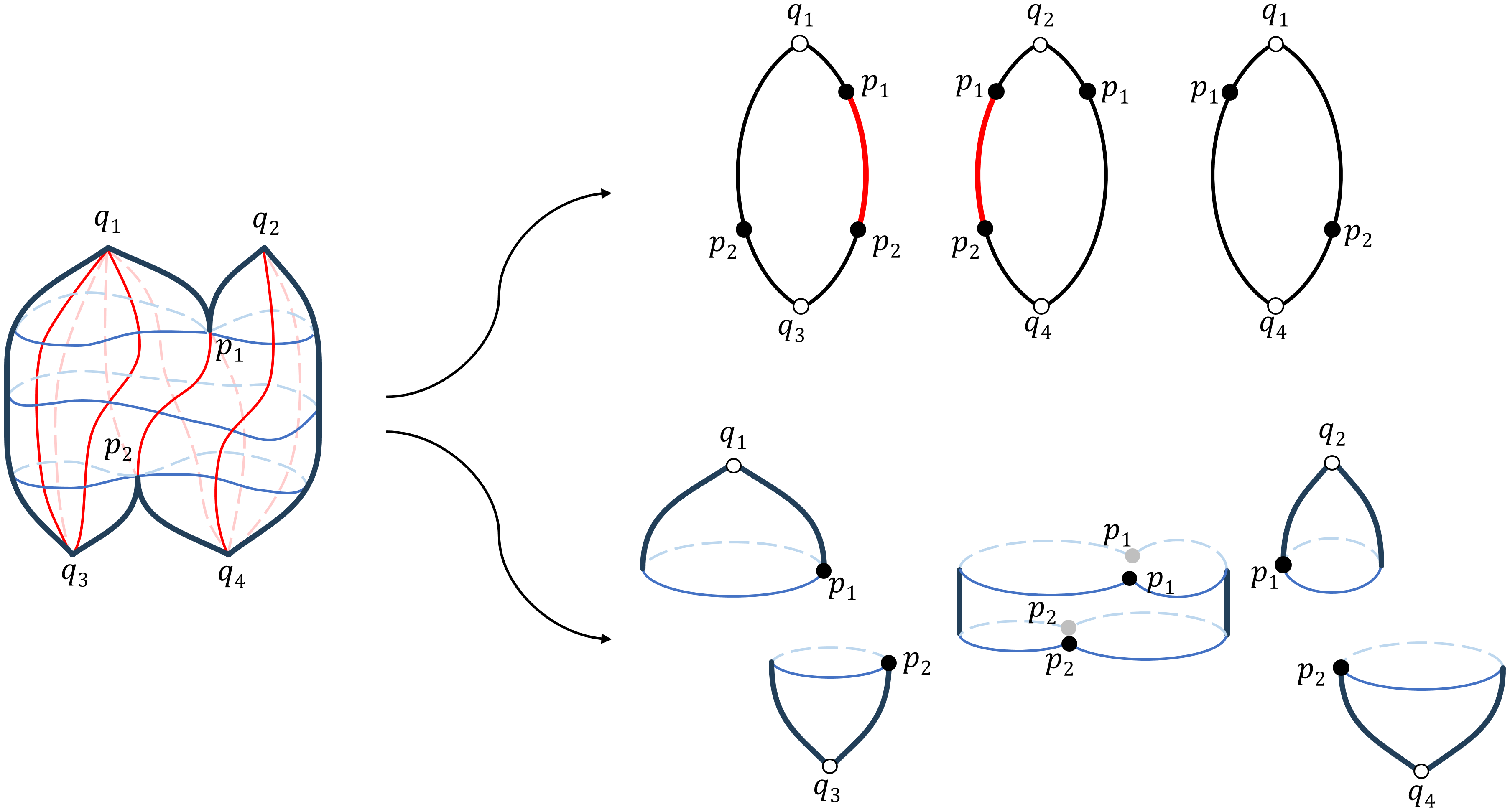
Figure 3: The strip decomposition (right top row) and annulus decomposition (right bottom row) of a foliated dihedral surface.

4.3 Sliding deformation

With the help of latitude and longitude foliations, we can define classes of geometric deformations.

Definition 4.10.

Let $(\Sigma_{1}\mathchar 24635\relax\;F_{1},G_{1})$, $(\Sigma_{2}\mathchar 24635\relax\;F_{2},G_{2})$ be two foliated dihedral surfaces with the same topological type and angle vector. They are said to be differed by a sliding deformation if there exists a homeomorphism $J:\Sigma_{1}\to\Sigma_{2}$ preserving the label, such that $G_{1}=J^{*}G_{2}$ as measured foliations on topological surfaces.

In other words, a sliding deformation of a foliated dihedral surface is changing the length of boundary segments while keeping the gluing pattern and widths of the bigons in strip decomposition.

The effect of sliding is changing the position of the zeros of $G$. Note that cones of angle $(2k-1)\pi$ must lie on the equatorial net, so sliding can only change the position of cone points of angle $2k\pi$. The angle vector is kept, and the underlying Riemann surface is usually changed.

This deformation is described geometrically and can be applied locally. It also includes a classes of global deformation discovered before.

It is observed in CWWX (15) that an abelian differential $\omega$ induces a 1-parameter family of co-axial metrics, expressed by the developing map

$$D_{\lambda}(z):=\lambda\cdot\exp\left(\int_{z_{0}}^{z}\omega\right):=\lambda\cdot D_{1}(z),\quad\lambda\in\mathbb{R}_{+}$$

as a multi-valued meromorphic function on $\Sigma-P$. We call changing the positive parameter the $\lambda$-deformation of co-axial surface. Note that the underlying Riemann surface and the angle vector are fixed and $D_{\lambda}(z)$ is always conformal.

The $\lambda$-deformation changes the radial distance from the origin while keep the argument. Thus the longitude foliation is kept during the deformation, and so does the gluing pattern of strip decomposition. The $0$ is always the developing image of north pole of each bigon. If $\left\lvert D_{1}(z)\right\rvert=r(z)$, then the spherical distance from $D_{1}(z)$ to $0$ is $\int_{0}^{r(z)}\frac{2\mathrm{d}w}{1+w^{2}}=2\arctan r(z)$. Thus the spherical distance from $D_{\lambda}(z)$ to $0$ is $2\arctan\left\lvert D_{\lambda}(z)\right\rvert=2\arctan(\lambda\cdot r(z))$. It is just a reassignment of the length of boundary segments of all bigons, thus a sliding deformation. See Figure 4. It is a global one and the accurate variation of the length depend on the location of the cone points.

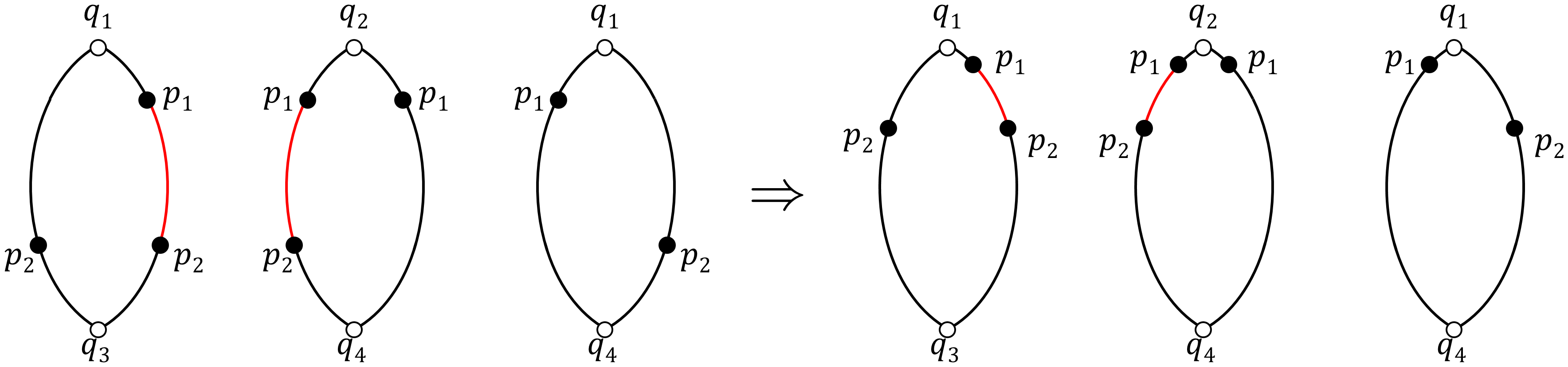
Figure 4: The effect of $\lambda$-deformation, which is a special case of sliding deformation.

Remark 4.11.

$D^{*}_{\lambda}(\mathbf{i}z/\mathrm{d}z)$ are the same 1-form on $\Sigma$ for all $\lambda>0$. So one can not distinguish the 1-parameter family of co-axial metrics differed by $\lambda$-deformation merely by 1-forms on a Riemann surface. Our modification on the transverse measure of $F$ fixes this problem by encoding more geometric information. So the moduli space of foliated surfaces is finer than the moduli space of 1-forms inducing co-axial metrics.

Remark 4.12.

We can consider the limiting surface1 when $\lambda\to 0$. The distance to the origin from any points other than $\infty$ tends to $0$, so we lost information about all cone points other than those mapped to $+\infty$. In terms of the strip decomposition, the only things remained is the number and width of bigons, with the gluing pattern of edges that ending at the south poles.

Hence we claim that the limit of $\lambda$-deformation of a co-axial surface is a singular surface obtained by gluing several footballs along one of their vertex. The number of footballs equals to the number of developing map preimages of $\infty$ on $\Sigma$. The case of $\lambda\to+\infty$ is similar. Such degenerated structures merit further investigation.

4.4 Splitting a pole

This deformation turns a pole of the foliation of angle $2k\pi$ into a zero of the same angle. It can be regarded as a special kind of sliding deformation.

Definition 4.13.

For $p\in P\cap Q$ of angle $2k\pi,k\in\mathbb{Z}_{>1}$, the split deformation slightly move it along $G$, so that the pole splits into $k$ poles which are smooth point on the surface, and the cone point becomes a zero of foliation with index $2-2k$. See Figure 5 and the geometric description below.

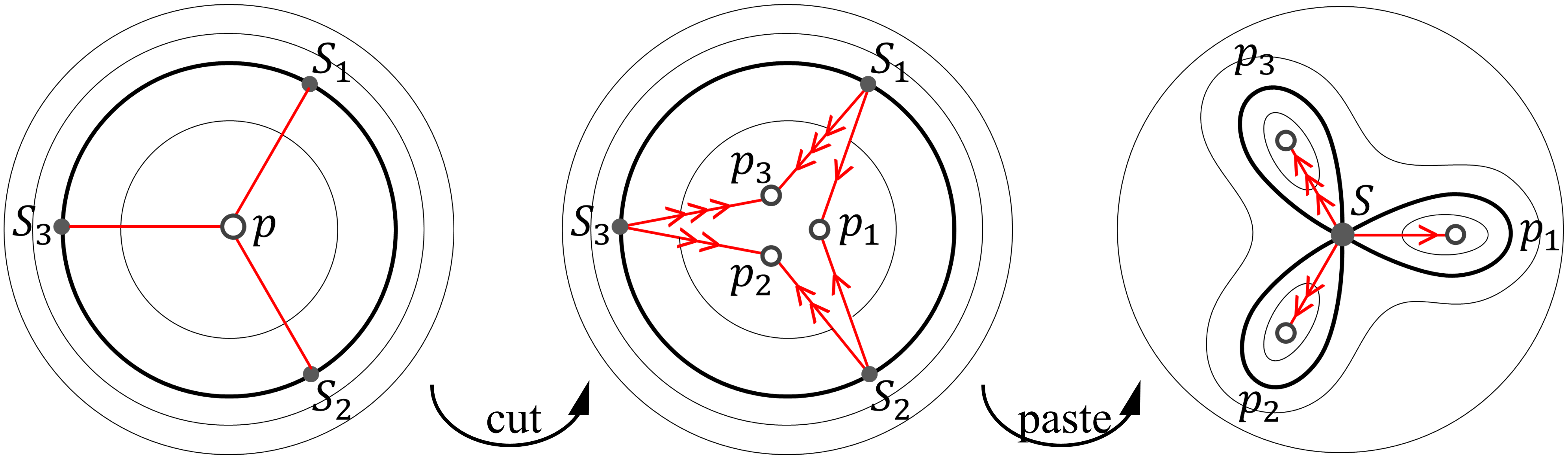
Figure 5: Splitting a pole of cone angle $6\pi$. Some leaves of $F$ is shown. Note the bold line that switch from a regular leaf to singular leaves.

Geometrically, this deformation is obtained by a cut-and-paste operation. One first pick $k$ isometric longitude segments $v_{1}=pS_{1},\cdots,v_{k}=pS_{k}$ from $p$, equally spaced by $2\pi$ angle. The length $\ell$ of these closed segments is small enough so that they contain no singularity other than $p$. Then cut the surface along $v_{i}$’s, one obtain a bordered surface with one boundary component. The cone point $p$ splits into $k$ boundary vertices $p_{1},\cdots p_{k}$. Suppose the vertices are $S_{1},p_{1},S_{2},p_{2},\cdots S_{k},p_{k},S_{1}$ in counterclockwise. Then glue $p_{i}S_{i}$ to $p_{i}S_{i+1}$ for all $i=1,\cdots,k$ (index mod $k$). The foliation structure matches naturally, because the boundary are leaf segments of $G$ and perpendicular to leaves of $F$. All $S_{i}$ are glued to a common point, which is the new cone point of angle $2k\pi$, and each $p_{i}$ becomes a pole.

Notice that there is a 2-dimensional choice when splitting a zero: the directions of the $k$ equally spaced segments, and the length of the segments.

This also appears in Ere20a , at the beginning of [Proof of Theorem 1].

Remark 4.14.

Actually this can be generalized to a local operation that splits a cone angle of $2\pi\theta$ into $k+1$ cone points of angle $2\pi\theta_{1},\cdots,2\pi\theta_{k},2k\pi$ with $\theta_{1}+\cdots+\theta_{k}=\theta$. This does not require dihedral condition since foliation works locally.

The effect of splitting a pole on the strip decomposition is a little bit more complicated. The $k$ picked segments $v_{i}$ lie on some leaf of $G$. If it is not in $\mathrm{Sing}(G)$, then cut the bigon containing it along this leaf and add two boundary marked points on each side corresponding to $S_{i}$. If it is in $\mathrm{Sing}(G)$, then it is already a boundary of two bigons. Also add two boundary marked points on each side corresponding to $S_{i}$. Now the gluing pattern of $p_{i}S_{i}$’s are given as above, and the pattern of other edges are the same before cutting. See Figure 6 as an example.

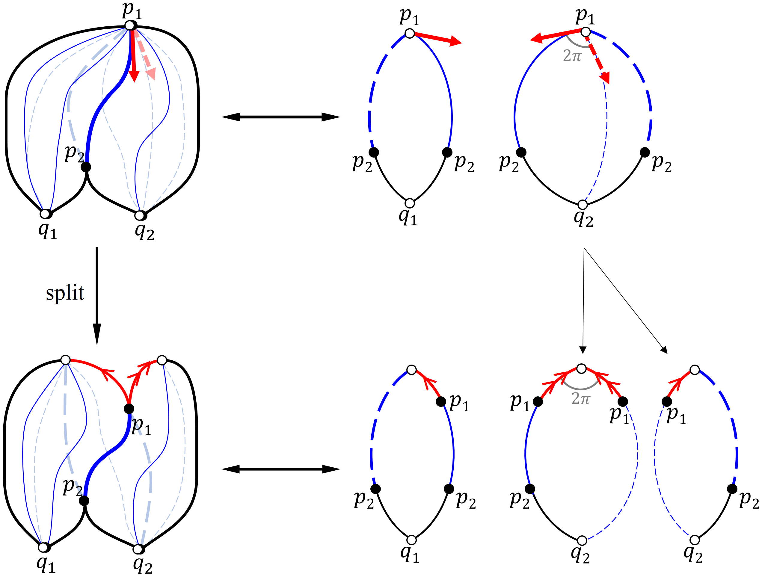
Figure 6: Split a pole of cone angle $4\pi$ on a dihedral four-cone sphere. The foliation $F$ is shown in blue. Right column shows the effect on strip decomposition. Note that one of the $v_{i}$ already lies on a singular leaf of $G$.

4.5 Twist deformation

Another type of deformation is “perpendicular” to the previous one. Namely, it preserve the latitude foliation. Basically this is the same as the twist in Fenchel-Nielsen coordinates for hyperbolic surfaces. See (Hub, 06, Section 7.6) for example. Flat version of twist also appears in literature. See (Gup, 15, Section 3.1) as an example.

Let $(\Sigma\mathchar 24635\relax\;F,G)$ be a dihedral spherical surface with annulus decomposition $\{B_{j}\}_{j=1}^{K}$. Suppose $B_{j}$ is not a punctured disk, with circumference $c_{j}=i(G,B_{j})$. Orient one boundary $\partial B_{j}^{+}$ such that the interior lies on the left, and let $f_{j}:\partial B_{j}^{+}\to\{r_{j}\mathrm{e}^{\mathbf{i}\theta}:r_{j}=c_{j}/2\pi\}$ be an isometric parameterization with respect to the transverse measure of $G$ on $\partial B_{j}^{+}$ and arc-length.

Definition 4.15.

A $\psi$-longitude (right) twisted surface about $B_{j}$ of $(\Sigma\mathchar 24635\relax\;F,G)$ is obtained by gluing the annulus with the same pattern as $\Sigma$, while every point on $\partial B_{j}^{+}$ is differed by a $-\psi$ translation. In the above parameterization, $x=f_{j}^{-1}(r_{j}\mathrm{e}^{\mathbf{i}\theta})\in\partial B_{j}^{+}$ is replaced with $x^{\prime}_{\psi}=f_{j}^{-1}(r_{j}\mathrm{}\mathrm{e}^{\mathbf{i}(\theta-2\pi\psi/c_{j})})$ when gluing.

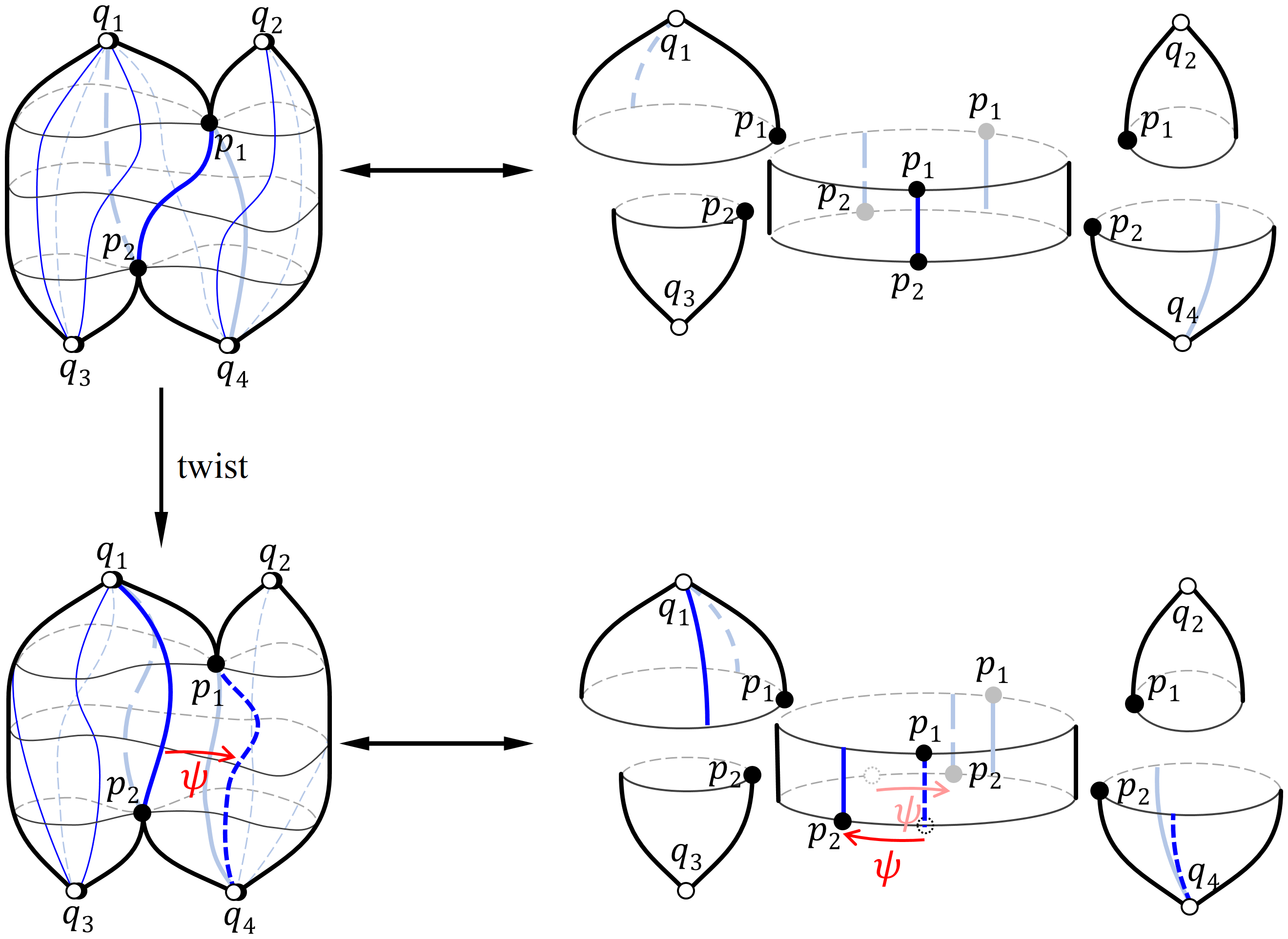
Figure 7: A positive twist about the center annulus. The longitude foliations are shown. Note that the strip decomposition changes. (It seems that $G$ is twisted to the left because a leaf segment is connected to some segment used to be on the left.)

In other words, we change how the leaves of $G$ match together when crossing the boundary of $B_{j}$. Intuitively, everything in $B_{j}$ is moving to the right when observe from $\partial B_{j}^{+}$, in the direction of $G$. Note that $F$ is fixed when twisting about an annulus. So we can say that two dihedral surface are differed by a twisting deformation if $F_{1}=F_{2}$ as measured foliations.

Remarks.

(1). The choice of $\partial B_{j}^{+}$ does not change the result: one boundary is moving the to right when seen from the other boundary.

(2). $\psi$ can take any real value. However, since we are studying the moduli space, the result are the same if the value are the same mod $c_{j}$, since we are studying the moduli space. So twist deformation is an $\mathbb{S}^{1}$-action.

Remark 4.16.

Twist can actually be defined in more general setting. Once there is a closed curve with constant geodesic curvature, possibly intersecting itself at cone points, and if no complementary component is isometric to some $S_{\theta}(r)$, then twisting deformation can be applied along this closed curve. The constant geodesic curvature condition is equivalent to that the developing map image of this closed curve in one analytic branch lies completely on one small circle. This seems to be the best analogue of the twist deformation in hyperbolic geometry so far.

4.6 Generic foliated surface

As an application of deformations defined before, we call talk how most dihedral surfaces look like. These surfaces have most independent parameters, so they form the top dimensional subset in the moduli space. We will focus on these surfaces later for the dimension count.

Definition 4.17.

A foliated dihedral surface $(\Sigma\mathchar 24635\relax\;F,G)$ is called generic if each boundary of the bigons in strip decomposition contains exactly one marked points. This is equivalent to the absence of vertical singular leaf connecting zeroes of $G$.

By strip decomposition, $(\Sigma\mathchar 24635\relax\;F,G)$ is determined by the width of bigons and the positions of marked points on the boundaries of bigons. So these geometric quantities and the gluing pattern of bigons completely parameterized the space of foliated surfaces. We now present an reversable deformation from a non-generic surface to a generic surface, so that non-generic surface can be regarded as the special case where some bigons in the strip decomposition have zero width. That is the reason for using the word “generic”.

Proposition 4.18.

Each foliated dihedral surface $(\Sigma\mathchar 24635\relax\;F,G)$ can be continuously deformed to a generic one with the same cone angle and of the same type.

Proof: One can apply sufficient times of twisting to avoid vertical saddle connecting in $G$. Since there are only finitely many cone points, if $(\Sigma\mathchar 24635\relax\;F,G)$ is non-generic then $G$ contains at most finitely many singular leaves connecting zeroes, which we call vertical saddle connection now. Let $\sigma$ be such a leaf, connecting cone points $p_{1},p_{2}$ (possibly the same) which are the zeros of $G$.

Now in the annulus decomposition of $(\Sigma\mathchar 24635\relax\;F,G)$ (See Definition 4.9 and Fig. 3), there exists an annulus $A=A(\sigma)$ passing through $\sigma$, with one boundary component $C_{1}\subset\partial A$ passing $p_{1}$. It can not be a punctured disk.

Consider all the singular leaves of $G$ intersecting $A$. Again there are only finitely many of them. These leaves, ending at singularities of $G$, must hit $C_{1}$. Then $C_{1}$ is divided into several open segments $I_{1},\cdots,I_{K}$ by these intersections. Denote longitude variation of $I_{j}$ by $d_{j}=i(I_{j},G)>0$. Let $t$ be a non-zero real number with $0<\left\lvert t\right\rvert<\min\{d_{1},\cdots,d_{K}\}$. Then a $t$-longitude (right) twist about $A$ will break the vertical saddle connection $\sigma$, and not produce new vertical saddle connection. See Figure 8. So we find a 1-parameter deformation of $(\Sigma\mathchar 24635\relax\;F,G)$ with fewer vertical saddle connections. The cone angles, the type of the new surfaces are all the same.

Finally by induction, one can break all vertical saddle connections without changing the cone angles and the type.

We remark that basically this is also done in (GT, 23, Proposition 3.5). Also note that the underlying complex structure usually changes.

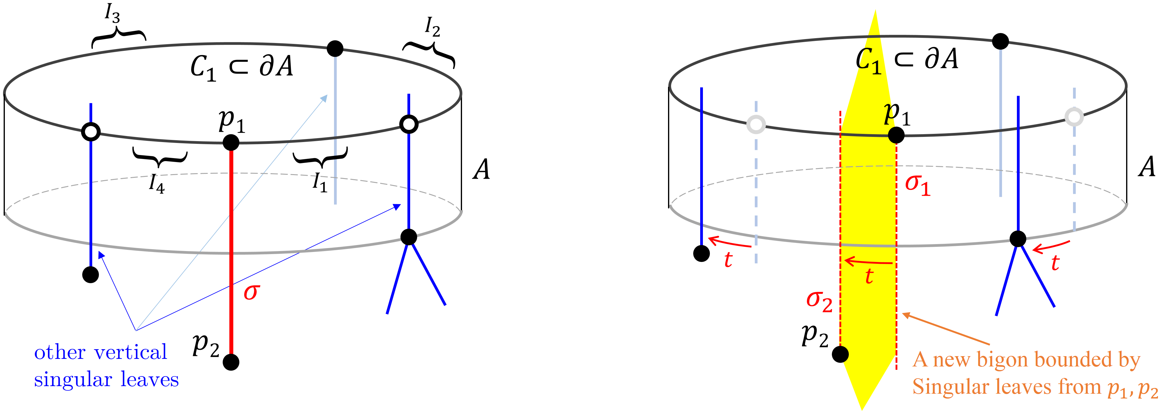
Figure 8: Twisting about an annulus to break vertical saddle connections. A new bigon appears after the deformation.

Corollary 4.19.

Non-generic foliated surfaces form a lower dimensional subset in $\mathcal{M}sphF_{g,n}^{D}(\vec{\theta}\mathchar 24635\relax\;\vec{T})$ or $\mathcal{M}sphF_{g,n}^{C}(\vec{\theta}\mathchar 24635\relax\;\vec{T})$ for every possible type partition $\vec{T}$.

Proof: After the twist deformation, the singular leaves from $p_{1}$ and $p_{2}$ in the direction of $\sigma$ mismatch at longitude variation $t$. By the choice of $t$, no other singular leaf lies in between them. So these two singular leaves cut off a bigon in new strip decomposition.

View the deformation in reverse order, the original foliated surface is obtained by shrinking the width of some bigon to zero. The more times twist deformation we applied to obtain a generic surface, the more bigons we need to shrink in the reverse. So non-generic surfaces have less parameters than generic ones.

Remark 4.20.

Randomly shrinking the width of bigons to zero may change the cone angles, and even degenerate the underlying surface. This is also the reason why the direction of contraction flow in (GT, 23, Proposition 3.5) should be generic. These lead to the infinite boundary of moduli space and will be topics of future research.

5 Dimension counting

To proof Theorem 1.1, we first study the fiber of projection from moduli space of foliated surfaces to unfoliated ones. Then independent parameters for foliated surface of given type is counted. Finally, we vary the type partition and obtain the dimension count. Strict dihedral and co-axial case are treated separately.$2g-2+n>0$ is assumed by default.

5.1 Identification lemma

Basically, identification lemma answers how many strip decomposition are identified to one surface in moduli space. Let us first take a look at the following interesting example, which shows the necessity of such lemma.

Example 5.1.

A generic foliated surface in $\mathcal{M}sphF_{1,1}^{D}(2)$ is glued by 2 bigons. The width $\theta_{1},\theta_{2}$ of the two bigons satisfying $\theta_{1}+\theta_{2}=\pi$ so that the vetices of bigons glued to a smooth point. The gluing pattern is shown in the left column of Figure 9.

However, there are two more choices of strip decomposition or foliation. The symmetry center of each bigon is the new pole of another foliation. The singular leaves of that longitude foliation on each bigon are also symmetric about its center. The middle and right column of Figure 9 shows how to cut the original bigons and glue to new ones. All blue and green arcs are geodesic segments.

Let $x,x^{\prime},x^{\prime\prime}$ be the length of the shorter boundary segment of bigons in each decomposition, and $\theta_{1},\theta^{\prime}_{1},\theta^{\prime\prime}_{1}$ be the width of the bigon whose shorter boundary segment lies on the left. By spherical geometry, they satisfy the equations

$$\left\{\begin{array}[]{lll}\cos x^{\prime}&=\sin x&\cos(\theta_{1}/2)\\ \cos x&=\sin x^{\prime}&\sin(\theta^{\prime}_{1}/2)\end{array}\right.,\quad\left\{\begin{array}[]{lll}\cos x^{\prime\prime}&=\sin x&\sin(\theta_{1}/2)\\ \cos x&=\sin x^{\prime\prime}&\cos(\theta^{\prime\prime}_{1}/2)\end{array}\right..$$

One can check that if $(x,\theta_{1})=(\arctan\sqrt{2},\pi/2)$, three decomposition are differed by a $\frac{2}{3}\pi$-rotation around $p$ and hence equivalent. Otherwise they are not equivalent. $\square$

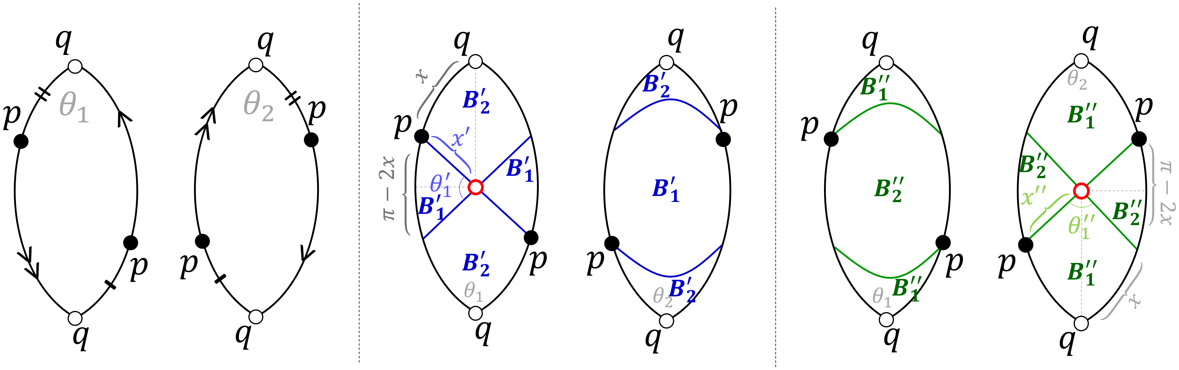
Figure 9: Three strip decomposition of a same spherical torus with one $4\pi$ cone point.

Remark. In fact $\mathcal{M}sph_{1,1}(2)=\mathcal{M}sph^{D}_{1,1}(2)$. Also see (EMP, 20, Theorem F.).

Before stating and proving the main proposition we make some settings. Every foliated surface is induced by some developing map. Suppose $\Sigma\in\mathcal{M}sph^{D}_{g,n}(\vec{\theta})$ admits more than one foliated surfaces, and let $(\Sigma\mathchar 24635\relax\;F,G)$ be one of them in $p^{-1}(\Sigma)\subset\mathcal{M}sphF_{g,n}^{D}(\vec{\theta})$ induced by developing map $D$, with monodromy group $\Gamma:=\rho_{D}(\pi_{1})$ (see Section 2.2). Every other developing map must be differed from $D$ by a $\mathrm{PSU}(2)$ element, and the monodromy group is differed by a conjugation. Thus finding another foliated surface is equivalent to finding some $g\in\mathrm{PSU}(2)$ such that $g\Gamma g^{-1}\subset\mathrm{O}(2)$. Let

$$G={\color[rgb]{0,0,0}G_{\Gamma}}:=\{\ \phi\in\mathrm{PSU}(2)\ \rvert\ \phi^{-1}\Gamma\phi\subset\mathrm{O}(2)\ \}.$$

Obviously, $\mathrm{O}(2)\subset G$. However, $G$ may not be a group. If $\phi,\psi\in G$, then $(\phi\psi)^{-1}\Gamma(\phi\psi)=\psi^{-1}(\phi^{-1}\Gamma\phi)\psi$. Thus $\phi\psi\in G_{\Gamma}$ if and only if $\psi\in G_{\phi^{-1}\Gamma\phi}$.

On the other hand, if $\phi\in G$, then for any $r\in\mathrm{O}(2)$, $\phi\circ r\in G$. So the exact set we want to study is the right quotient $G/\mathrm{O}(2)$.

Proposition 5.2 (Identification lemma for strict dihedral surface).

For strict dihedral $(\Sigma\mathchar 24635\relax\;F,G)$, $\#\{G/\mathrm{O}(2)\}$ is 1 or 3. And $\#\{G/\mathrm{O}(2)\}=3$ if and only if $\Gamma$ is isomorphic to the Klein-4 group $K4:=\mathbb{Z}_{2}\times\mathbb{Z}_{2}$.

In other words, $\#\{p^{-1}(\Sigma)\}\leq 3$ for all $\Sigma\in\mathcal{M}sph^{D}_{g,n}(\vec{\theta})$.

Proof: Suppose $G\neq\mathrm{O}(2)$.

(1). We pick a representative for an element in $G/\mathrm{O}(2)$.

If $\phi:z\mapsto\frac{az+b}{-\bar{b}z+\bar{a}}$, then

$$[\phi]:=\phi\cdot\mathrm{O}(2) =\left\{\ z\mapsto\frac{a\mathrm{e}^{\mathbf{i}\theta}z+b}{-\bar{b}\mathrm{e}^{\mathbf{i}\theta}z+\bar{a}},\quad z\mapsto\frac{a\mathrm{e}^{\mathbf{i}\theta}+bz}{-\bar{b}\mathrm{e}^{\mathbf{i}\theta}+\bar{a}z}\ \bigg{\rvert}\ \theta\in\mathbb{R}\ \right\}$$

$$=\left\{\ z\mapsto\frac{a\mathrm{e}^{\mathbf{i}\theta/2}z+b\mathrm{e}^{-\mathbf{i}\theta/2}}{-\bar{b}\mathrm{e}^{\mathbf{i}\theta/2}z+\bar{a}\mathrm{e}^{-\mathbf{i}\theta/2}},\quad z\mapsto\frac{b\mathrm{e}^{\mathbf{i}(\pi-\theta)/2}z+a\mathrm{e}^{\mathbf{i}(\pi+\theta)/2}}{\bar{a}\mathrm{e}^{\mathbf{i}(\pi-\theta)/2}z-\bar{b}\mathrm{e}^{\mathbf{i}(\pi+\theta)/2}}\ \bigg{\rvert}\ \theta\in\mathbb{R}\ \right\}.$$

Thus $\pm ab$ is the invariant of an element in $G/\mathrm{O}(2)$ in terms of $\mathrm{PSU}(2)$ representation. And $\phi\in\mathrm{O}(2)\Leftrightarrow ab=0$. So whenever $\phi\notin\mathrm{O}(2)$, we can choose a representative of $[\phi]$ such that $a>0$ and $\arg(b)\in[0,\pi)$.

(2). $\Gamma$ keeps a pair of antipodal points other than North and South poles.

Pick non-trivial $[\phi]\in G/\mathrm{O}(2)$, represented by $\phi:z\mapsto\frac{az+b}{-\bar{b}z+\bar{a}}$ with $a>0$ and $\arg(b)\in[0,\pi)$. Then $\phi\{0,\infty\}=\{b/\bar{a},-a/\bar{b}\}\neq\{0,\infty\}$. Thus

$$\Gamma\{b/\bar{a},-a/\bar{b}\}=\Gamma\phi\{0,\infty\}=\phi\big{(}\phi^{-1}\Gamma\phi\{0,\infty\}\big{)}=\phi\{0,\infty\}=\{b/\bar{a},-a/\bar{b}\}.$$

So $\Gamma$ keeps two different pairs of antipodal points.

(3). The rotation subgroup $\Gamma_{0}:=\Gamma\cap\mathrm{U}(1)$ must be $\mathbb{Z}_{2}$, so $\Gamma\cong K4$.

$\Gamma_{0}$ can not be trivial. Otherwise for any $\gamma,\gamma^{\prime}\in\Gamma-\mathrm{U}(1)$, $\gamma\gamma^{\prime}\in\Gamma\cap\mathrm{U}(1)=\{\mathrm{id}\}$. However, every $\gamma\in\Gamma-\mathrm{U}(1)$ is an order-2 element, or $\gamma^{2}=\mathrm{id}$. Thus there is only one element in $\Gamma-\mathrm{U}(1)$ and $\Gamma\cong\mathbb{Z}_{2}$, contradicting strict dihedral condition.

Now let $\psi\in\Gamma_{0}$ non-trivial, and assume $\psi:z\mapsto\mathrm{e}^{\mathbf{i}\theta}z,\ \theta\in\mathbb{R}-2\pi\mathbb{Z}$. Then $\psi$ should fix the antipodal points $\{b/\bar{a},-a/\bar{b}\}\neq\{0,\infty\}$. This implies $\psi=\gamma_{0}:=z\mapsto-z$. Then $\Gamma_{0}=\{\mathrm{id},\gamma_{0}\}$, and $\Gamma$ has 4 elements. Since all elements in $\Gamma-\Gamma_{0}$ is order-2, $\Gamma\cong K4$. We have

$$\Gamma=\{\ \mathrm{id},\ z\mapsto\mathrm{e}^{\mathbf{i}\theta}/z,\ z\mapsto-z,\ z\mapsto-\mathrm{e}^{\mathbf{i}\theta}/z\ \}.$$

Let $g_{\theta}:z\mapsto\mathrm{e}^{\mathbf{i}\theta/2}z$, then it is always conjugated to the standard $K4$ in $\mathrm{PSU}(2)$:

$$g_{\theta}^{-1}\Gamma g_{\theta}=\{\ \mathrm{id},\ z\mapsto 1/z,\ z\mapsto-z,\ z\mapsto-1/z\ \}:=K.$$

So we shall now assume that $\Gamma=K$ as above.

(4). Solving non-trivial $[\phi]\in G/\mathrm{O}(2)$.

Since $\Gamma$ also keeps $\{b/\bar{a},-a/\bar{b}\}\neq\{0,\infty\}$, and the only fixed points of $\gamma_{0}:z\mapsto-z$ are $0,\infty$, we have $b/\bar{a}=a/\bar{b}$. Then $\left\lvert a\right\rvert^{2}=\left\lvert b\right\rvert^{2}=1/2$, and $a=1/\sqrt{2}$ by normalization. Let $b=\mathrm{e}^{\mathbf{i}\beta}/\sqrt{2},\ 0\leqslant\beta<\pi$. Then $\{b/\bar{a},-a/\bar{b}\}=\{\pm\mathrm{e}^{\mathbf{i}\beta}\}$ is invariant under $z\mapsto 1/z$.

a). $1/\mathrm{e}^{\mathbf{i}\beta}=-\mathrm{e}^{\mathbf{i}\beta}$. Then $\beta=\pi/2$. We have

$$\phi_{1}=\frac{z+\mathbf{i}}{\mathbf{i}z+1}.$$

b).$1/\mathrm{e}^{\mathbf{i}\beta}=\mathrm{e}^{\mathbf{i}\beta}$. Then $\beta=0$. We have

$$\phi_{2}=\frac{z+1}{-z+1}.$$

So if $G/\mathrm{O}(2)$ is non-trivial, $\Gamma\cong K4$ and there will be 2 non-trivial elements $[\phi_{1}],[\phi_{2}]\in G/\mathrm{O}(2)$ given above. The reverse automatically holds by Step (4).

In $\mathrm{SO}(3,\mathbb{R})$, $\phi_{1},\phi_{2}$ are the $\pi/2$-rotation about the $x,y$-axis, and $\gamma_{0}$ is the $\pi$-rotation about the $z$-axis. We can re-state the result in different languages.

Corollary 5.3.

1. Let $K\subset\mathrm{PSU}(2)$ and $\phi_{1},\phi_{2}\in\mathrm{PSU}(2)$ as above. Then $K,\phi_{1}^{-1}K\phi_{1},\phi_{2}^{-1}K\phi_{2}$ are three subgroups of $\mathrm{O}(2)$ which are conjugate in $\mathrm{PSU}(2)$ but not in $\mathrm{O}(2)$.

2. Let $\Sigma$ be a strict dihedral surface whose monodromy group is isomorphic to $K4$. Then regarded as a Riemann surface, there exists at least two distinct meromorphic quadratic differentials on it, with all real periods, that shares the same set of zeros and simple poles.

5.2 Connection matrix

There are as many linear equations on the widths of bigons as the number of poles. The connection matrix helps us detect their linearly independence. The idea is the same as Li (19) used for co-axial surfaces.

Let $(\Sigma\mathchar 24635\relax\;F,G)$ be a generic foliated surface, with $m$ poles $\{q_{1},\cdots,q_{m}\}$ of $F$. Assume its strip decomposition consists of $b$ bigons $\{B_{1},\cdots,B_{b}\}$.

Definition 5.4.

The connection matrix $\mathbf{M}$ of $(\Sigma\mathchar 24635\relax\;F,G)$ is an $m\times b$ matrix with all entries in $\{0,1,2\}$, determined by the following:

• if both vertices of bigon $B_{j}$ are glued to one pole $q_{i}$, then $\mathbf{M}_{ij}:=2$ ;

• if vertices of $B_{j}$ are glued to different poles $q_{i}\neq q_{i^{\prime}}$, then $\mathbf{M}_{ij}=\mathbf{M}_{i^{\prime}j}:=1$;

• all the other entries are $0$.

Since each bigon has exactly two vertex, each column of $\mathbf{M}$ contains 1 or 2 non-zero entries, with total sum 2. Let $\vec{C}:=(c_{1},\cdots,c_{m})^{T}$ be the column vector recording cone angles of $q_{i}$ on $\Sigma$, and $\vec{W}:=(w_{1},\cdots,w_{b})^{T}$ be the vector recording widths of $B_{j}$. Then the constrain on the widths of bigons is given by

$$\vec{C}=\mathbf{M}\vec{W}.$$ (5.1)

Proposition 5.5.

1. $\mathrm{rank}(\mathbf{M})\geqslant m-1$.

2. The foliation pair $(F,G)$ is orientable if and only if $\mathrm{rank}(\mathbf{M})=m-1$.

The key is the connectedness of $\mathbf{M}$ observed in Li (19). We include a proof here for convenience.

Lemma 5.6.

For generic $(\Sigma\mathchar 24635\relax\;F,G)$, its connection matrix $\mathbf{M}$ is path-connected in the following sense: for any two non-zero elements $\mathbf{M}_{ij},\mathbf{M}_{kl}$, there exists a finite sequence $(i_{0},j_{0}),(i_{1},j_{1}),\cdots,(i_{N},j_{N})$ such that

• $(i_{0},j_{0})=(i,j),(i_{N},j_{N})=(k,l)$;

• $(i_{t-1},j_{t-1}),(i_{t},j_{t})$ have exactly one same component for all $t=1,\cdots,N$;

• all entries $\mathbf{M}_{(i_{t},j_{t})}$ are non-zero.

Proof: This is related to the connectedness of the surface. Up to a re-labeling of the poles and bigons, we may assume $\mathbf{M}_{11},\mathbf{M}_{kl}\neq 0$ and $k,l\neq 1$. Choose a path $\sigma$ on $\Sigma$ from an interior point in $B_{1}$ to an interior point in $B_{l}$, avoiding all singularity of $F$. Then consider all the bigons, assumed to be $B_{j_{1}}=B_{1},B_{j_{2}},\cdots,B_{j_{L}}=B_{l}$, along the path $\sigma$. Whenever $\sigma$ goes into $B_{j_{i+1}}$ from $B_{j_{i}}$, these two bigons glued to a common pole because the foliated surface is generic. Then there exists a desired sequence among the columns of $B_{j_{1}},\cdots,B_{j_{L}}$.

Remark. The connection matrix in Li (19) is always connected, while ours may not be connected for non-generic surfaces. These two matrices encode “dual” information: Li’s is obtained from annulus decomposition while ours is induced by strip decomposition. So the information of intermediate annulus is completely missing here, possibly breaking the connectedness.

Proof: [Proof of Proposition 5.5. ]

(1). We show that if $\mathrm{rank}(\mathbf{M})<m-1$, then $\mathbf{M}$ is not path-connected. In that situation, any $m-1$ rows of $\mathbf{M}$ are linearly dependent. Up to re-labeling, we may assume that there exists non-zero $\lambda_{i},\ i=1,\cdots,r$ such that $\sum_{i=1}^{r}\lambda_{i}\vec{M}_{i}=0$, where $\vec{M}_{i}$ is the $i$-th row of $\mathbf{M}$, $r\leq m-1$.

Now pick any non-zero entry $\mathbf{M}_{xy}$ on the last $m-r$ row (i.e., $r<x\leq m$). Such entry exists because any pole has positive cone angle. Note that the total sum of each column is 2. If $\mathbf{M}_{xy}=2$, then $\mathbf{M}_{iy}=0$ for all $i\neq x$. If $\mathbf{M}_{xy}=1$, then there exists a uniqe $x^{\prime}\neq x$ with $\mathbf{M}_{x^{\prime}y}=1$, and $\mathbf{M}_{iy}=0$ for all $i\neq x,x^{\prime}$. However, the first $r$ rows are linear dependent so $\sum_{i=1}^{r}\lambda_{i}\mathbf{M}_{iy}=0$, with all $\lambda_{i}\neq 0$. Thus $x^{\prime}>r$.

So for all $j=1,\cdots,b$, if $1\leq i\leq r$ and $r+1\leq i^{\prime}\leq m$, them $\mathbf{M}_{ij},\mathbf{M}_{i^{\prime}j}$ can not be simultaneously non-zero. This means the entries in the first $r$ rows and ones in the last $m-r$ rows are not path-connected, a contradiction.

(2). We show that the orientation induces a linear equation. Note that as a pair of topological foliation induced by some meromorphic differentials, $F,G$ must be orientable or non-orientable simultaneously.

When $(F,G)$ is orientable, the two vertices of each bigon glues to different poles, and all non-zero entries of $\mathbf{M}$ is $1$. Pick one orientation of $F$. Then for each $B_{j}$, we can tell which vertex lies on the left or right of $F$, and it is well-defined all over the surface. Define $\lambda_{i}=+1$ if $q_{i}$ lies on the left of $F$, otherwise define $\lambda_{i}=-1$. Then we immediately see $\sum_{i=1}^{m}\lambda_{i}\vec{M}_{i}=0$, since each bigon is glued to exactly one pole on the left and one pole on the right. So $\mathbf{M}$ is not full-rank, then $\mathrm{rank}(\mathbf{M})$ must be $m-1$.

Conversely, if $\mathrm{rank}(\mathbf{M})=m-1<m$, then there exists non-zero $\lambda_{i}$ such that $\sum_{i=1}^{m}\lambda_{i}\vec{M}_{i}=0$. As before, there is no 2 in $\mathbf{M}$, otherwise it is the only non-zero entry on that column and the coefficient $\lambda_{i}$ for that row must be 0. Similarly, for each column there is exactly two non-zero entry, both equal to 1. Then coefficients $\lambda_{i}$ for that two rows must be opposite each other. By the connectedness of $\mathbf{M}$, all $\lambda_{i}$ have the same absolute value. Then we shall assume that $\lambda_{i}=\pm 1$.

An orientation of $F$ can be given by the following. On each bigon, orient the restriction of $F$ so that the pole with positive $\lambda_{i}$ lies on the left. This orientation matches piece by piece, since all bigons glued to the same poles are recorded on one row, with the same coefficient. And the linear equation guarantees the two poles to which a bigon is glued lie on different side of $F$. As a sequence, if $\Sigma$ is strict dihedral, then the connection matrix must be full-rank, for all possible strip decomposition.

Example 5.7.

The connection matrix, together with the equations, for two strip decomposition in Example 4.6 is

$$\begin{pmatrix}1/2\\ 1/2\\ 1\\ 1\end{pmatrix}=\begin{pmatrix}1&&\\ &&1\\ 1&1&\\ &1&1\\ \end{pmatrix}\begin{pmatrix}1/2\\ 1/2\\ 1/2\end{pmatrix}\quad\text{ and }\quad\begin{pmatrix}1\\ 1\\ 1\end{pmatrix}=\begin{pmatrix}2&1&&\\ &1&1&\\ &&1&2\\ \end{pmatrix}\begin{pmatrix}\theta\\ 1-2\theta\\ 2\theta\\ 1/2-\theta\end{pmatrix}$$

$\square$

5.3 Dimension count for strict dihedral case

Now we can count the dimension of $\mathcal{M}sphF_{g,n}^{D}(\vec{\theta}\mathchar 24635\relax\;\vec{T})$.

Theorem 5.8.

Let $\vec{\theta}:=(\theta_{1},\cdots,\theta_{n})\in\mathbb{R}^{n}_{+}$ be an angle vector with $\theta_{i}\neq 1$ and $\vec{T}=\{E,O,N\}$ be a type partition with $\#E=n_{E},\#O=n_{O},\#N=n_{N}$. If $\mathcal{M}sphF_{g,n}^{D}(\vec{\theta}\mathchar 24635\relax\;\vec{T})$ is non-empty, then its real dimension is

$$2n_{E}+n_{O}+2g-2.$$

A (global but may not faithful) geometric coordinate is given by the width of bigons in the strip decomposition, together with the absolute latitude of the zeros of even index.

Proof: We only need to consider generic surfaces as mentioned in 4.6. Suppose that there are $b$ bigons in the strip decomposition, and $m\geq 0$ extra poles in $Q-P$.

By the definition of Euler characteristic we have

$$2-2g=(n_{E}+n_{O}+n_{N}+m)-2b+b$$

for generic surface. Then $b=m+n+(2g-2)$.

Now that every zero of even index provide one parameter, namely its absolute latitude. Every zero of odd index must lie on the equatorial net, thus do not provide new parameter.

The widths of $B$ bigons are the other real parameters, constrained by $n_{N}+m$ linear equations $\vec{C}=\mathbf{M}\vec{W}$, where $\mathbf{M}$ is the $(n_{N}+m)\times b$ connection matrix. By Proposition 5.5, for strict dihedral surface, $\mathbf{M}$ is full-rank. Then the dimension of the solution space of the widths vector $\vec{W}$ is

$$b-\mathrm{rank}(\mathbf{M})=\big{(}m+n+(2g-2)\big{)}-\big{(}n_{N}+m\big{)}=n-n_{N}+2g-2.$$

Together with the parameters provided by the zeros of even index, if the foliated moduli space of type $\vec{T}$ is non-empty, the total dimension is

$$n_{E}+(n-n_{N}+2g-2)=2n_{E}+n_{O}+2g-2.$$

We may also consider the dimension of $\mathcal{M}sph^{D}_{g,n}(\vec{\theta})$, which is the maximal dimension of $\mathcal{M}sph_{g,n}^{D}(\vec{\theta}\mathchar 24635\relax\;\vec{T})$ among all possible type partition $\vec{T}$.

Definition 5.9.

Given an angle vector $\vec{\theta}$, the maximal type partition $\vec{T}_{0}$ is defined to be the type partition $\{E_{0},O_{0},N_{0}\}$ such that

$$T:=\sum_{i\in E_{0}\sqcup O_{0}}\theta_{i}\text{ is integer and maximal.}$$

Denote $\#E_{0}=M_{E},\#O_{0}=M_{O},\#N_{0}=M_{N}$. Then $M_{O}$ must be even. We use upper case $M$ for maximal partition and lower case $n$ for general partition.

For the maximal type partition, all indexes with integer angle is in $E_{0}$. If the total number of half-integers is even, all their indexes are in $O_{0}$. If the number is odd, $O_{0}$ contains all but the index of the smallest half-integer.

$T$ is called the maximal integral sum in GT (23). A necessary condition for the existence of dihedral surface, called strengthened Gauss-Bonnet inequalities, is given in terms of $T$ and $g,n$ there.

Theorem 5.10.

Let $\vec{\theta}:=(\theta_{1},\cdots,\theta_{n})\in\mathbb{R}^{n}_{+}$ be an angle vector with $\theta_{i}\neq 1$, and let $\vec{T}_{0}$ be the maximal type partition as above. Then whenever the moduli space is non-empty, the maximal dimension of $\mathcal{M}sph^{D}_{g,n}(\vec{\theta})$ is

$$2M_{E}+M_{O}+2g-2.$$

Proof: This heavily relies on the proof in GT (23). Gendron-Tahar showed that whenever $\mathcal{M}sph^{D}_{g,n}(\vec{\theta})$ is non-empty, one can find a strict dihedral surface with maximal type partition $\vec{T}_{0}$. So $\mathcal{M}sph_{g,n}^{D}(\vec{\theta}\mathchar 24635\relax\;\vec{T}_{0})$ is non-empty, with the desired dimension.

5.4 Dimension count for co-axial case

Now we study the vertical arrows in (3.4) of co-axial surfaces.

A developing map is determined by its behavior on an open set. Thus whenever $N\neq\emptyset$ in the type partition $\vec{T}$, the projection $p_{T}$ is injective. So we only need to consider the case where $N=\emptyset$.

If $N=\emptyset$ in the co-axial case, all $\theta_{i}\in\mathbb{N}_{>1}$. As before, everything depend on the monodromy group.

Lemma 5.11 (Identification lemma for co-axial surfaces).

Suppose $N=\emptyset$ in the type partition.

1. If the monodromy group of $\Sigma$ is trivial, then $p_{T}^{-1}(\Sigma)$ is a two-dimensional fiber in $\mathcal{M}sphF_{g,n}^{C}(\vec{\theta}\mathchar 24635\relax\;\vec{T})$.

2. If the monodromy group of $\Sigma$ is not trivial, then the foliated surface in $\mathcal{M}sphF_{g,n}^{C}(\vec{\theta}\mathchar 24635\relax\;\vec{T})$ with orientable $(F,G)$ is unique.

Proof: When the monodromy is trivial, the developing map induces a branched cover directly from $\Sigma$ to $\mathbb{S}^{2}$. Then composing any $\mathrm{PSU}(2)$ element on the left still pulls back the foliation. To fix type, the preimages of poles must be disjoint from the cone points. This is an open condition for the $\mathrm{PSU}(2)$ elements. Finally the quotient $\mathrm{PSU}(2)/\mathrm{O}(2)$ is 2-dimensional.

For the second statement, following notations in Proposition 5.2, with $\Gamma=\Gamma_{0}\subset\mathrm{U}(1)$ this time. By step (2) and (3) there, $G/\mathrm{O}(2)$ must be trivial if $\Gamma$ is not $\mathbb{Z}_{2}$ or trivial group.

If $\Gamma\cong\mathbb{Z}_{2}$, then up to a conjugation we may assume $\Gamma=\{\mathrm{id},\ \gamma_{0}:z\mapsto-z\}$. Let $\phi\in\mathrm{PSU}(2)$ as before, with $ab\neq 0$. Then

$$\phi^{-1}\gamma_{0}\phi:z\mapsto\frac{(\left\lvert a\right\rvert^{2}-\left\lvert b\right\rvert^{2})z+2\bar{a}b}{2a\bar{b}z+(\left\lvert b\right\rvert^{2}-\left\lvert a\right\rvert^{2})}.$$

This is in $\mathrm{O}(2)$ if and only if $\bar{a}b(\left\lvert a\right\rvert^{2}-\left\lvert b\right\rvert^{2})=0$. Thus $a=1/\sqrt{2}$ and $b=\mathrm{e}^{\mathbf{i}\beta}/\sqrt{2},\ 0\leqslant\beta<\pi$ as before. One can check that

$$\phi=\frac{z+\mathrm{e}^{\mathbf{i}\beta}}{-\mathrm{e}^{-\mathbf{i}\beta}z+1},\quad\phi^{-1}\gamma_{0}\phi=\frac{\mathrm{e}^{2\mathbf{i}\beta}}{z}$$

satisfies the requirements for all $\beta\in[0,\pi)$. However, this new element lies in $\mathrm{O}(2)-\mathrm{U}(1)$, thus the induced foliation is non-orientable. This is forbidden in $\mathcal{M}sphF_{g,n}^{C}(\vec{\theta}\mathchar 24635\relax\;\vec{T})$. So the choice of orientable $(F,G)$ is actually unique.

As a corollary, if the monodromy group of $\Sigma$ is $\mathbb{Z}_{2}$, then this cone spherical metric is induced by both a unique 1-form and a 1-parameter family of primitive quadratic differentials. This is exactly the case of Example 4.6.

However, the appearance of trivial monodromy is not very often. It depends on the genus.

Proposition 5.12.

Suppose $\vec{\theta}\in\mathbb{Z}_{>1}^{n}$ and $N=\emptyset$ in the type partition $\vec{T}$.

• If genus is zero, then any $\Sigma\in\mathcal{M}sph^{C}_{0,n}(\vec{\theta})$ has trivial monodromy.

• If genus $g>0$, then the surfaces with trivial monodromy form a lower dimensional subset in $\mathcal{M}sph_{g,n}^{C}(\vec{\theta}\mathchar 24635\relax\;\vec{T})$.

Proof: When $g=0$, the simple primitive closed loops around each cone point generate $\pi_{1}(\Sigma^{\prime})$. Thus when all cone angles are integers, the monodromy group is trivial.

We prove the second statement for foliated moduli space $\mathcal{M}sphF_{g,n}^{C}(\vec{\theta}\mathchar 24635\relax\;\vec{T})$ first. Since non-generic foliated surfaces already form a lower-dimensional subset, we shall only consider generic foliated surfaces. We study the extra constrains on the width vector imposed by the trivial monodromy condition.

(1). Some homology preparations are needed.

Fix an orientation of latitude foliation $F$. For each bigon $B_{j}$ in the strip decomposition, pick an interior segment $e_{j}$ connecting the two boundary marked points, and orient it along $F$. Each $B_{j}$ is cut into two pieces by $e_{j}$, and all half-pieces sharing a same pole $q_{l}$ glued to a topological disk $d_{l}$. The cone points $\{p_{i}\}_{i=1}^{n}$, the segments $\{e_{j}\}_{j=1}^{b}$, and the disks $\{d_{l}\}_{l=1}^{m}$ around the poles, form a cell complex structure for $\Sigma$. Here $m>0$ is the number of poles of $F$.

Since $\mathrm{U}(1)$ is abelian, $\mathrm{Hom}(\pi_{1}(\Sigma^{\prime}),\mathrm{U}(1))=\mathrm{Hom}(H_{1}(\Sigma^{\prime}),\mathrm{U}(1))$. When all $\theta_{i}\in\mathbb{Z}$, the closed loops around every cone point have trivial monodromy. So we can consider the homology group $H_{1}(\Sigma)$ instead. Then the oriented segments $\{e_{j}\}$ form a basis of the chain group $C_{1}(\Sigma)$. The effect on the monodromy of moving along $e_{j}$ is a $2\pi w_{j}$-rotation.

Let $a_{1},\cdots,a_{2g}$ be a canonical basis of $H_{1}(\Sigma)$. Then as closed 1-chains, there exists a $2g\times b$ integer matrix $X$ such that

$$\begin{pmatrix}a_{1}\\ \vdots\\ a_{2g}\end{pmatrix}=X\begin{pmatrix}e_{1}\\ \vdots\\ e_{b}\end{pmatrix}$$

with $\mathrm{rank}(X)=2g$. Suppose $\rho$ is the monodromy representation of $(\Sigma\mathchar 24635\relax\;F,G)$. For $\gamma\in H_{1}(\Sigma)$, let $(\ln\rho)(\gamma):=\psi\in[0,1)$ if $\rho(\gamma)=z\mapsto e^{2\pi\mathbf{i}\psi}\in\mathrm{U}(1)$. Then we have

$$\ln\rho\begin{pmatrix}a_{1}\\ \vdots\\ a_{2g}\end{pmatrix}\equiv X\begin{pmatrix}w_{1}\\ \vdots\\ w_{b}\end{pmatrix}\quad(\text{mod }\mathbb{Z}).$$

On the other hand, since $F$ is orientable, the connection matrix contains no entry 2, and we can improve it with signature. As in the proof of Proposition 5.5, step (2), if $B_{j}$ glued to pole $q_{i}$ that lies on the left of $F$, one define $\mathbf{M}_{ij}=+1$; if $q_{i}$ lies on the right of $F$, one define $\mathbf{M}_{ij}=-1$. Then the total sum of each column in this $\mathbf{M}$ is 0. The boundary chain of each disk $d_{l}$ consists of segments with same signature. So we can orient them properly so that

$$\begin{pmatrix}\partial d_{1}\\ \vdots\\ \partial d_{m}\end{pmatrix}=\mathbf{M}\begin{pmatrix}e_{1}\\ \vdots\\ e_{b}\end{pmatrix},$$

where $\partial:C_{2}(\Sigma)\to C_{1}(\Sigma)$ is the boundary operator.

Since $a_{1},\cdots,a_{2g}$ generates $H_{1}(\Sigma)$, they must be linearly independent at chain level. So rows of $X$ are all independent. However, each row of $\mathbf{M}$ gives a boundary chain. So each row of $X$ is linearly independent of all rows in $\mathbf{M}$.

(2). If $\vec{W}_{0}\in\mathbb{R}_{\geqslant 0}^{b}$ is the width vector of some generic foliated surface $(\Sigma\mathchar 24635\relax\;F,G)$ with trivial monodromy, then there exists $\vec{C}_{0}\in\mathbb{Z}_{+}^{m}$ and $\vec{A}\in\mathbb{Z}^{2g}$ such that

$$\vec{C}_{0}=\mathbf{M}\vec{W}_{0},\quad\vec{A}=X\vec{W}_{0}.$$ (5.2)

We show that the dimension of solution space is strictly smaller than $(b-\mathrm{rank}(\mathbf{M}))$.

By Proposition 5.5, $\mathrm{rank}(\mathbf{M})=m-1$. Let $\boldsymbol{M}_{1},\cdots,\boldsymbol{M}_{m-1}$ be $(m-1)$ linearly independent rows of $\mathbf{M}$, and $\boldsymbol{X}_{1},\cdots,\boldsymbol{X}_{2g}$ be the rows of $X$. Suppose these rows are linearly dependent, then there exists $\lambda_{1},\cdots,\lambda_{m-1},\mu_{1},\cdots,\mu_{2g}$ such that

$$\lambda_{1}\boldsymbol{M}_{1}+\cdots+\lambda_{m-1}\boldsymbol{M}_{m-1}=\mu_{1}\boldsymbol{X}_{1}+\cdots+\mu_{2g}\boldsymbol{X}_{2g}.$$

Multiplying this equation on the basis $\left(e_{1},\cdots,e_{b}\right)^{T}$, the left side becomes a linear combination of $\partial d_{1},\cdots,\partial d_{m}$, which must be exact. And the right side becomes a linear combination of the homology basis $a_{1},\cdots,a_{2g}$, which can not be exact. Then both sides are zero. Since $\boldsymbol{M}_{i}$’s are linearly independent, all $\lambda_{i}$ is zero. Thus

$$\mathrm{rank}\begin{pmatrix}\mathbf{M}\\ X\end{pmatrix}\geq m-1+2g$$

and the solution space of (5.2) has dimension $\leq b-(m-1+2g)<b-(m-1)$. So we have proved the second statement for $\mathcal{M}sphF_{g,n}^{C}(\vec{\theta}\mathchar 24635\relax\;\vec{T})$.

(3). Finally, we project the result to the moduli space of unfoliated surfaces. There are three kinds of situations in $\mathcal{M}sphF_{g,n}^{C}(\vec{\theta}\mathchar 24635\relax\;\vec{T})$: non-generic surfaces, generic surface with trivial monodromy, generic surface with non-trivial monodromy. We have shown in Proposition 4.18 that non-generic surfaces form lower dimensional subset (possibly also have trivial monodromy). Step (2) above shows that generic surfaces with non-trivial monodromy form subset of codimension at lest $2g>0$. Thus generic surfaces with non-trivial monodromy form a top-dimensional subset.

On the other hand, the projection $p_{T}:\mathcal{M}sphF_{g,n}^{C}(\vec{\theta}\mathchar 24635\relax\;\vec{T})\to\mathcal{M}sph_{g,n}^{C}(\vec{\theta}\mathchar 24635\relax\;\vec{T})$ does not increase the dimension. And by Lemma 5.11-(2) $p_{T}$ preserves dimension on the subset of generic surfaces with non-trivial monodromy. So this subset has top dimension in both moduli space.

Finally, we can state the dimension count for co-axial surfaces.

Theorem 5.13.

Let $\vec{\theta}=(\theta_{1},\cdots,\theta_{n})\in\mathbb{R}^{n}_{+}$ be an angle vector with $\theta_{i}\neq 1$ and $\vec{T}=\{E,N\}$ be a type partition with $\#E=n_{E},\#N=n_{N}$. Whenever $\mathcal{M}sph_{g,n}^{C}(\vec{\theta}\mathchar 24635\relax\;\vec{T})$ is non-empty, its real dimension is given by the following:

• If $g>0$, the dimension is $2n_{E}+2g-1$;

• If $g=0$ and $N$ non-empty, the dimension is $2n_{E}-1$;

• If $g=0$ and $N$ empty, then $\vec{\theta}\in\mathbb{N}_{>1}^{n}$ and the dimension is $2n-3$.

Remark. It is possible $\mathcal{M}sph_{g,n}^{C}(\vec{\theta}\mathchar 24635\relax\;\vec{T}_{1})=\mathcal{M}sph_{g,n}^{C}(\vec{\theta}\mathchar 24635\relax\;\vec{T}_{2})$ for $\vec{T}_{1}\neq\vec{T}_{2}$.

Proof: (1). If $g>0$, by Proposition 5.12.(2) and Lemma 5.11.(2), $p_{T}$ in (3.4) is injective on some open subset. So we only need to count the dimension of $\mathcal{M}sphF_{g,n}^{C}(\vec{\theta}\mathchar 24635\relax\;\vec{T})$.

As before, assume there are $b$ bigons in the strip decomposition and $m\geq 0$ more poles of the latitude foliation. We have $b=n+m+(2g-2)$. However, since we require the foliations to be orientable, the rank of connection matrix $\mathbf{M}$ must be $n_{P}+m-1$ by Proposition 5.5. Then the real dimension of $\mathcal{M}sphF_{g,n}^{C}(\vec{\theta}\mathchar 24635\relax\;\vec{T})$ is

$$n_{E}+(b-\mathrm{rank}(\mathbf{M}))=n_{E}+b-(n_{P}+m-1)=2n_{E}+2g-1.$$

If $g=0$ while $N\neq\emptyset$, $p_{T}$ is automatically injective and above arguments hold.

(2). If $g=0$ and $N=\emptyset$, then by Proposition 5.12.(1) and Lemma 5.11.(1), $\mathcal{M}sph_{0,n}^{C}(\vec{\theta}\mathchar 24635\relax\;\vec{T})$ is two-dimension lower than $\mathcal{M}sphF_{0,n}^{C}(\vec{\theta}\mathchar 24635\relax\;\vec{T})$. And previous dimension count for the foliated moduli space holds. Thus its real dimension is

$$(2n_{E}+2g-1)-2=2n-3.$$

We can also consider the maximal dimension of $\mathcal{M}sph^{C}_{g,n}(\vec{\theta})$. This is simpler than the strict dihedral case.

Theorem 5.14.

Let $\vec{\theta}:=(\theta_{1},\cdots,\theta_{n})\in\mathbb{R}^{n}_{+}$ be an angle vector with $\theta_{i}\neq 1$. Suppose there are $N_{E}$ integers and $N_{N}$ non-integers. Then the dimension of $\mathcal{M}sph^{C}_{g,n}(\vec{\theta})$ is

$$\left\{\begin{array}[]{ll}2N_{E}+2g-1&,\text{ if }(g,N_{N})\neq(0,0)\mathchar 24635\relax\\ 2n-3&,\text{ if }(g,N_{N})=(0,0).\\ \end{array}\right.$$

Proof: Let $\vec{T}=\{E,N\}$ be a type partition. Then whenever $N$ contains a cone with integer angle, we can split this pole and move it into $E$. By finitely many steps, $N$ contains no integer cone. So the desired dimension is achieved.

In other words, all other moduli spaces $\mathcal{M}sph_{g,n}^{C}(\vec{\theta}\mathchar 24635\relax\;\vec{T})$ appear at the boundary of the moduli space $\mathcal{M}sph^{C}_{g,n}(\theta\mathchar 24635\relax\;\vec{T}_{0})$ with maximal type partition $\vec{T}_{0}=\{E_{0},N_{0}\}$ where $E_{0}$ contains all integer cone points.

Remark. Note that Li (19) has counted the real dimension of moduli space of Strebel 1-form being $2g+l-1$, where $l=n_{E}$ is the number of zeros. The extra $n_{E}$ dimensions just come from the sliding deformation of the zeros along longitude foliation.

5.5 Examples for distinct type partitions

The final part contains two examples of moduli space with the same prescribed cone angle but different type.

Example 5.15.

Let $g=1,n=3,\vec{\theta}=(4,\frac{1}{2},\frac{3}{2})$. Consider two type partitions

$$\vec{T}_{A}:=\left(\{4\}\mathchar 24635\relax\;\{\frac{1}{2},\frac{3}{2}\}\mathchar 24635\relax\;\emptyset\right)\text{ and }\vec{T}_{B}:=\left(\{4\}\mathchar 24635\relax\;\emptyset\mathchar 24635\relax\;\{\frac{1}{2},\frac{3}{2}\}\right).$$

Then $\mathcal{M}sph^{D}_{1,3}(\vec{\theta}\mathchar 24635\relax\;\vec{T}_{A})$ and $\mathcal{M}sph^{D}_{1,3}(\vec{\theta}\mathchar 24635\relax\;\vec{T}_{B})$ has a one-dimensional intersection.

Proof: . By Theorem 5.8,

$$\dim_{\mathbb{R}}\mathcal{M}sph^{D}_{1,3}(\vec{\theta}\mathchar 24635\relax\;\vec{T}_{A})=4,\quad\dim_{\mathbb{R}}\mathcal{M}sph^{D}_{1,3}(\vec{\theta}\mathchar 24635\relax\;\vec{T}_{B})=2.$$

They are non-empty once we construct their intersection. If $\Sigma$ lies in their intersection, there exists at least two different choices of $(F,G)$ on $\Sigma$. By Proposition 5.2, its monodromy group must be $K4$. Using methods similar in the proof of Proposition 5.12, we can show that the surfaces with $K4$-monodromy also form a lower dimensional subset. So the intersection of $\mathcal{M}sph^{D}_{1,3}(\vec{\theta}\mathchar 24635\relax\;\vec{T}_{A})$ and $\mathcal{M}sph^{D}_{1,3}(\vec{\theta}\mathchar 24635\relax\;\vec{T}_{B})$ is at most one dimensional.

On the other hand, we can precisely found a one-dimensional subset as the following Figure 10. We are not considering the behavior of different components, but at least these two subspace must must have one-dimensional intersection, while their own dimension are different.

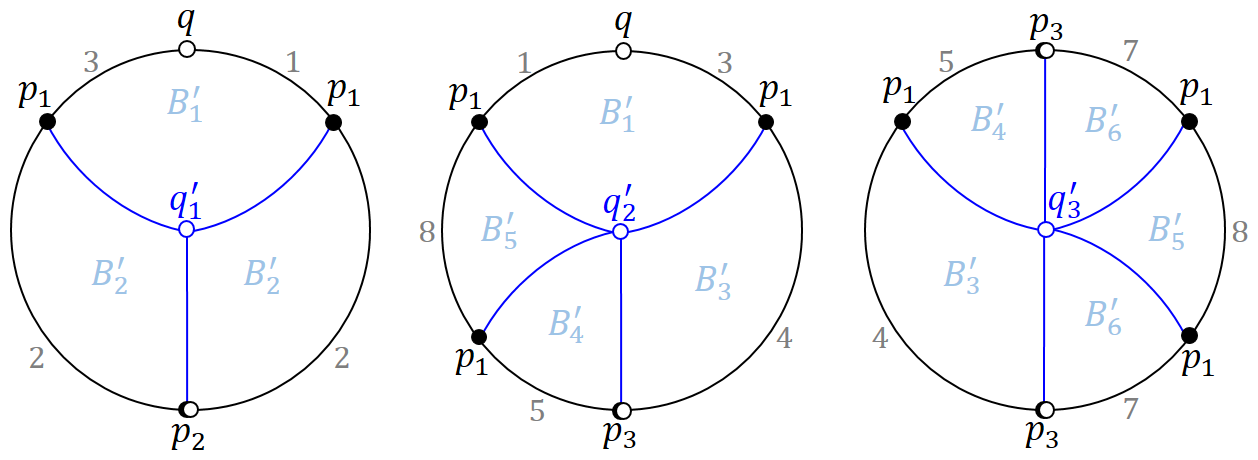
Figure 10: Strip decomposition of a surface in the intersection of two moduli space of different type. The first decomposition, draw in black, consists of 3 hemispheres and is of type $\vec{T}_{B}$. The second one, draw in blue, consists of 6 bigons and is of type $\vec{T}_{A}$. The one-parameter is the absolute latitude of $p_{1}$.

Example 5.16.

Now let $g=1,n=4,\vec{\theta}^{\prime}=(4,\frac{1}{2},\frac{3}{2},c)$, where $c$ is an irrational number with $\frac{1}{2}<c<2$. Consider type partitions

$$\vec{T}^{\prime}_{A}:=(\{4\}\mathchar 24635\relax\;\{\frac{1}{2},\frac{3}{2}\}\mathchar 24635\relax\;\{c\})\text{ and }\vec{T}^{\prime}_{B}:=(\{4\}\mathchar 24635\relax\;\emptyset\mathchar 24635\relax\;\{\frac{1}{2},\frac{3}{2},c\}).$$

In this case $\mathcal{M}sph^{D}_{1,4}(\vec{\theta}^{\prime}\mathchar 24635\relax\;\vec{T}^{\prime}_{A})$ and $\mathcal{M}sph^{D}_{1,4}(\vec{\theta}^{\prime}\mathchar 24635\relax\;\vec{T}^{\prime}_{B})$ are disjoint in $\mathcal{M}sph^{D}_{1,4}(\vec{\theta}^{\prime})$.

Proof: Firstly, both moduli spaces are non-empty. And since $c$ is irrational, it must be a pole of the foliation. Thus the choice of $(F,G)$ is unique for each $\Sigma\in\mathcal{M}sph^{D}_{1,4}(\vec{\theta}^{\prime})$. Note that $\vec{T}^{\prime}_{A}$ is the maximal type partition, so by Gendron-Tahar’s proof it can be realized.

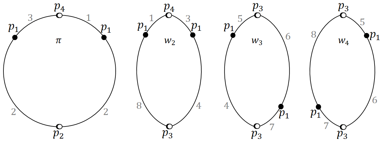
Figure 11: One gluing pattern for $\mathcal{M}sph^{D}_{1,4}(\vec{\theta}^{\prime}\mathchar 24635\relax\;\vec{T}^{\prime}_{B})$, where $\frac{1}{2}+w_{2}=c,\ w_{2}+2(w_{3}+w_{4})=\frac{3}{2}$.

These examples imply the connected component worth serious study. This also provides a reason for studying several strata of meromorphic quadratic differentials simultaneously, and their relative position.

We end with a summary. A co-axial spherical metric must be induced by some special meromorphic 1-form on the underlying Riemann surface. And its monodromy induces a pair of latitude and longitude foliation. However, the relations between these there objects are subtle.

Unitary 1-form can not represent all co-axial surface, because the $\lambda$-deformation keeps the whole conformal structure, and can only be detected by spherical geometry. Yet the total space of measured foliation pairs, which captures both the meromorphic object and geometric structure, is slightly superfluous. There can be several choices of foliations on one surface. Thus the moduli space of co-axial spherical surfaces is something in between them. This fact faithfully exhibit the fun and difficulty of cone spherical surfaces, even in this particular case.

🖂 Sicheng Lu

The Institute of Geometry and Physics, University of Science and Technology of China, Hefei 230026 China

Email address: sichenglu@ustc.edu.cn

Bin Xu

School of Mathematical Sciences and CAS Wu Wen-Tsun Key Laboratory of Mathematics, University of Science and Technology of China, Hefei 230026 China

Email address: bxu@ustc.edu.cn

References

- BDMM (11) Daniele Bartolucci, Francesca De Marchis, and Andrea Malchiodi. Supercritical conformal metrics on surfaces with conical singularities. Int. Math. Res. Not. IMRN, (24):5625–5643, 2011.
- CKL (17) Zhijie Chen, Ting-Jung Kuo, and Chang-Shou Lin. Existence and non-existence of solutions of the mean field equations on flat tori. Proc. Amer. Math. Soc., 145(9):3989–3996, 2017.
- CLW (15) Ching-Li Chai, Chang-Shou Lin, and Chin-Lung Wang. Mean field equations, hyperelliptic curves and modular forms: I. Camb. J. Math., 3(1-2):127–274, 2015.
- CWWX (15) Qing Chen, Wei Wang, Yingyi Wu, and Bin Xu. Conformal metrics with constant curvature one and finitely many conical singularities on compact Riemann surfaces. Pacific J. Math., 273(1):75–100, 2015.
- dBP (22) Martin de Borbon and Dmitri Panov. Parabolic bundles and spherical metrics. Proc. Amer. Math. Soc., 150(12):5459–5472, 2022.
- EG (15) Alexandre Eremenko and Andrei Gabrielov. On metrics of curvature 1 with four conic singularities on tori and on the sphere. Illinois J. Math., 59(4):925–947, 2015.
- EGT (14) Alexandre Eremenko, Andrei Gabrielov, and Vitaly Tarasov. Metrics with conic singularities and spherical polygons. Illinois J. Math., 58(3):739–755, 2014.
- EMP (20) Alexandre Eremenko, Gabriele Mondello, and Dmitri Panov. Moduli of spherical tori with one conical point. arXiv e-prints, arXiv:2008.02772, August 2020.
- Ere (04) A. Eremenko. Metrics of positive curvature with conic singularities on the sphere. Proc. Amer. Math. Soc., 132(11):3349–3355, 2004.
- (10) Alexandre Eremenko. Co-axial monodromy. Ann. Sc. Norm. Super. Pisa Cl. Sci. (5), 20(2):619–634, 2020.
- (11) Alexandre Eremenko. Metrics of constant positive curvature with four conic singularities on the sphere. Proc. Amer. Math. Soc., 148(9):3957–3965, 2020.
- Ere (21) Alexandre Eremenko. Metrics of constant positive curvature with conic singularities. A survey. arXiv e-prints, arXiv:2103.13364, March 2021.
- FLPe (91) A. Fathi, F. Laudenbach, V. Poenaru, and al. et. Travaux de Thurston sur les surfaces. Société Mathématique de France, Paris, 1991. Séminaire Orsay, Reprint of ıt Travaux de Thurston sur les surfaces, Soc. Math. France, Paris, 1979.
- GT (23) Quentin Gendron and Guillaume Tahar. Dihedral monodromy of cone spherical metrics. Illinois J. Math., 67(3):457–483, 2023.
- Gup (14) Subhojoy Gupta. Asymptoticity of grafting and Teichmüller rays. Geom. Topol., 18(4):2127–2188, 2014.
- Gup (15) Subhojoy Gupta. On the asymptotic behavior of complex earthquakes and Teichmüller disks. In Geometry, groups and dynamics, volume 639 of Contemp. Math., pages 271–287. Amer. Math. Soc., Providence, RI, 2015.
- Hei (62) Maurice Heins. On a class of conformal metrics. Nagoya Math. J., 21:1–60, 1962.
- Hub (06) John Hamal Hubbard. Teichmüller theory and applications to geometry, topology, and dynamics. Vol. 1. Matrix Editions, Ithaca, NY, 2006. Teichmüller theory, With contributions by Adrien Douady, William Dunbar, Roland Roeder, Sylvain Bonnot, David Brown, Allen Hatcher, Chris Hruska and Sudeb Mitra, With forewords by William Thurston and Clifford Earle.
- Li (19) Bo Li. Singular metrics of constant curvature and the heat flow of almost complex structures. PhD thesis, University of Science and Technology of China, 2019.
- LSX (21) Lingguang Li, Jijian Song, and Bin Xu. Irreducible cone spherical metrics and stable extensions of two line bundles. Adv. Math., 388:Paper No. 107854, 36, 2021.
- LT (92) Feng Luo and Gang Tian. Liouville equation and spherical convex polytopes. Proc. Amer. Math. Soc., 116(4):1119–1129, 1992.
- LW (10) Chang-Shou Lin and Chin-Lung Wang. Elliptic functions, Green functions and the mean field equations on tori. Ann. of Math. (2), 172(2):911–954, 2010.
- LW (17) Chang-Shou Lin and Chin-Lung Wang. Mean field equations, hyperelliptic curves and modular forms: II. J. Éc. polytech. Math., 4:557–593, 2017.
- McO (88) Robert C. McOwen. Point singularities and conformal metrics on Riemann surfaces. Proc. Amer. Math. Soc., 103(1):222–224, 1988.
- MP (16) Gabriele Mondello and Dmitri Panov. Spherical metrics with conical singularities on a 2-sphere: angle constraints. Int. Math. Res. Not. IMRN, (16):4937–4995, 2016.
- MP (19) Gabriele Mondello and Dmitri Panov. Spherical surfaces with conical points: systole inequality and moduli spaces with many connected components. Geom. Funct. Anal., 29(4):1110–1193, 2019.
- MW (17) Rafe Mazzeo and Hartmut Weiss. Teichmüller theory for conic surfaces. In Geometry, analysis and probability, volume 310 of Progr. Math., pages 127–164. Birkhäuser/Springer, Cham, 2017.
- MZ (20) Rafe Mazzeo and Xuwen Zhu. Conical metrics on Riemann surfaces I: The compactified configuration space and regularity. Geom. Topol., 24(1):309–372, 2020.
- MZ (22) Rafe Mazzeo and Xuwen Zhu. Conical metrics on Riemann surfaces, II: Spherical metrics. Int. Math. Res. Not. IMRN, (12):9044–9113, 2022.
- Pic (05) E. Picard. De l’intégration de l’équation sur une surface de Riemann fermée. J. Reine Angew. Math., 130:243–258, 1905.
- Poi (98) H. Poincaré. Les fonctions fuchsiennes et l’équation . Journal de Mathématiques Pures et Appliquées, 5e série, 4, 1898.
- PT (07) Athanase Papadopoulos and Guillaume Théret. On Teichmüller’s metric and Thurston’s asymmetric metric on Teichmüller space. In Handbook of Teichmüller theory. Vol. I, volume 11 of IRMA Lect. Math. Theor. Phys., pages 111–204. Eur. Math. Soc., Zürich, 2007.
- SCLX (20) Jijian Song, Yiran Cheng, Bo Li, and Bin Xu. Drawing cone spherical metrics via Strebel differentials. Int. Math. Res. Not. IMRN, (11):3341–3363, 2020.
- Str (84) Kurt Strebel. Quadratic differentials, volume 5 of Ergebnisse der Mathematik und ihrer Grenzgebiete (3) [Results in Mathematics and Related Areas (3)]. Springer-Verlag, Berlin, 1984.
- Tah (22) Guillaume Tahar. Geometric decompositions of surfaces with spherical metric and conical singularities. Q. J. Math., 73(2):657–678, 2022.
- Thu (97) William P. Thurston. Three-dimensional geometry and topology. Vol. 1, volume 35 of Princeton Mathematical Series. Princeton University Press, Princeton, NJ, 1997. Edited by Silvio Levy.
- Tro (89) Marc Troyanov. Metrics of constant curvature on a sphere with two conical singularities. In Differential geometry (Peñíscola, 1988), volume 1410 of Lecture Notes in Math., pages 296–306. Springer, Berlin, 1989.
- Tro (91) Marc Troyanov. Prescribing curvature on compact surfaces with conical singularities. Trans. Amer. Math. Soc., 324(2):793–821, 1991.
- UY (00) Masaaki Umehara and Kotaro Yamada. Metrics of constant curvature with three conical singularities on the -sphere. Illinois J. Math., 44(1):72–94, 2000.
- WWX (22) Zhiqiang Wei, Yingyi Wu, and Bin Xu. The structure of CSC-1 reducible conformal metrics on a compact Riemann surface with finite conical singularities. arXiv e-prints, arXiv:2211.11929, November 2022.