Using Bayesian Optimization to Design Time Step Size Controllers with Application to Modified Patankar–Runge–Kutta Methods

Abstract

Modified Patankar–Runge–Kutta (MPRK) methods are linearly implicit time integration schemes developed to preserve positivity and a linear invariant such as the total mass in chemical reactions. MPRK methods are naturally equipped with embedded schemes yielding a local error estimate similar to Runge–Kutta pairs. To design good time step size controllers using these error estimates, we propose to use Bayesian optimization. In particular, we design a novel objective function that captures important properties such as tolerance convergence and computational stability. We apply our new approach to several MPRK schemes and controllers based on digital signal processing, extending classical PI and PID controllers. We demonstrate that the optimization process yields controllers that are at least as good as the best controllers chosen from a wide range of suggestions available for classical explicit and implicit time integration methods.

MSC Classification]65L05, 65L50, 65L20

1 Introduction

Numerically solving systems of ordinary differential equations (ODEs)

$$\mathbf{y}^{\prime}(t)=\mathbf{f}(\mathbf{y}(t),t),\quad\mathbf{y}(0)=\mathbf{y}^{0},$$ (1)

gives rise to many challenges which are addressed theoretically by topics such as order of accuracy and convergence, stability, efficiency, and the preservation of linear invariants or further properties of the solution such as positivity.

Runge–Kutta (RK) methods are commonly used examples of numerical methods solving the initial value problem (1), and all the above mentioned topics have been excessively studied in the past, see for instance [1, 2, 3]. In this work, we are particularly interested in the aspect of efficiency using time step control.

Traditionally, the first step size control mechanism for numerical approximations of ODEs uses an estimate of the local error and multiplies the current time step size by a factor derived from the estimate to maximize the time step size while keeping the error below a given tolerance [2, Section II.4]. This approach is basically a deadbeat I controller and can be improved, in particular when the method is not operating in the asymptotic regime of small time step sizes. By including some history of the control process, improved PI controllers were introduced in [4, 5] and extended to more general digital signal processing (DSP) controllers in [6, 7]. For a deeper insight to this topic we refer also to [8, 9, 10, 11, 12]. In those publications general, time control theoretical arguments are used to deduce stable controllers. However, given a specific scheme, there is hope to further improve the time step control. One example is given in [13], where the authors equip RK methods with “optimized” DSP time step controllers. To that end, the authors sampled the domain of the hyperparameters from the controller and deduced the “optimal” parameters for the given test problems by means of minimizing the maximum, the median, or the $95\%$ percentile of the right-hand side evaluations followed by a final choice based on human interaction.

It is the purpose of this work to exclude the human interaction by incorporating ideas from Bayesian optimization [14, 15, 16]. The main benefit of this approach, besides human resources and failure, is that no expensive grid search is needed anymore, since the Bayesian optimization detects regions in the space of the hyperparameters resulting in an expensive, yet bad time step controller. Additionally, the tool will recognize which of the hyperparameters have larger impact on the performance of the controller — and which have not — so that the search is somewhat efficient. Of course, the term bad must be declared to the optimization tool. Indeed, the major obstacle in this approach is to come up with an appropriate cost function. Our approach of constructing such a cost function is to take into account many aspects a human would consider when analyzing work precision diagrams. To validate that the proposed cost function is a reasonable choice, we will compare the search result with standard parameters from the literature and built-in solvers from Matlab for a wide range of problems.

Another aspect of this work will be the application of the novel approach to a certain class of time integrators, which are motivated as follows. A major drawback of RK methods as a subclass of general linear methods [3, 17] is the order constraint for unconditional positivity, meaning that there exist only first-order accurate RK methods capable of producing positive approximations for $\mathbf{y}^{0}>\mathbf{0}$ and arbitrarily large time step sizes [18, 19]. The preservation of positivity, however, is a desirable property for many problems such as chemical reactions because negative approximations can lead to the failure of the method, see for instance [20] and the literature mentioned therein. To give an example in the context of partial differential equations (PDEs), the calculation of the speed of sound when solving the compressible Euler equations requires the positivity of pressure and density. Another system of PDEs that emphasizes the importance of generating positive approximations is given in [21], where the right-hand side of the so-called NPZD model (reviewed in Section A) introduced in [22] was used as stiff source terms. In the numerical solution of the resulting PDE, the occurrence of negative approximations can lead to the divergence of the method and therefore necessitates a severe time step constraint for methods that are not unconditionally positive. One approach to dealing with schemes that may produce negative approximations is to introduce limiters that result in time step restrictions [23]. Alternatively, different postprocessing techniques can be applied after each time step of a standard time integration method to enforce positivity [24, 25]. Other approaches are less rigorous and replace negative values by their magnitude or even by zero, which is also called clipping.

Another popular approach is to apply the Patankar trick [26, Section 7.2-2] to an RK method, resulting in a Patankar–Runge–Kutta (PRK) scheme, which guarantees the unconditional positivity of the numerical approximation. However, the PRK method in general does not preserve linear invariants anymore, which may lead to a qualitatively different behavior compared to schemes preserving all linear invariants [27]. Still, it is possible to improve the PRK method obtaining modified PRK (MPRK) schemes introduced in [28], which additionally are unconditionally conservative, meaning that the sum of the constituents of the numerical approximation remains constant for all steps and any chosen time step size.

We note that MPRK methods are linearly implicit and that performing the modified Patankar (MP) trick on an RK scheme does not result in an RK method. Even more, MPRK schemes do not belong to the class of general linear methods. Thus, the rich theory for RK schemes cannot be applied directly to deduce the properties of MPRK methods. As a result, the construction of second- and third-order MPRK schemes [29, 30] was interlinked with technical proofs using Taylor series expansions. Recently, a new approach generalizing the theory of NB-series [31] was presented in [32] providing a technique for systematically deriving conditions for arbitrary high order nonstandard additive Runge–Kutta (NSARK) methods to which MPRK schemes belong.

The above approach can also be applied to different time integrators to construct further unconditionally positive and conservative schemes. For instance, using Deferred Correction (DeC) methods as a starting point, the MP approach led to MPDeC schemes, which are conservative, unconditionally positive, and of arbitrary high order [33]. These schemes were also used to preserve a positive water height when solving the shallow water equations [34]. Further positivity-preserving schemes are discussed in [35, 36, 23, 37].

Due to the nonlinear nature of these Patankar-type methods, a stability analysis for several members of this family of schemes was not available until recently [38, 39, 40, 41, 42], where the local behavior near steady states of linear autonomous problems was investigated using the theory of discrete dynamical systems. We also want to note that some issues of Patankar-type schemes were discussed in [43], where different modified Patankar methods from [33, 29, 30] were analyzed with respect to oscillatory behavior. Furthermore, a necessary condition for avoiding these oscillations was given in [44].

Altogether, up to now the theory for order of consistency and convergence as well as stability of RK schemes was adapted to MPRK methods. Moreover, the schemes are also proven to be unconditionally positive and conservative. However, MPRK methods have not yet been improved with respect to their efficiency. Up to now, only standard step size controllers were used for a particular PRK method [45]. However, the construction of a tailored time step controller is still missing. This is the purpose of the present work.

Here, we focus on DSP controllers (reviewed in Section 3) to investigate several MPRK schemes which we recall in Section 2. We explain our methodology in Section 4, where we also introduce our cost function. For the search of an optimal controller, we consider multiple test problems described in Section A of the appendix, each of which challenges the DSP controller in a different way. We derive tailored controller parameters and validate the resulting methods with further test problems introduced in Section B of the appendix, leading to the improved controllers described in Section 5. Finally, we summarize our findings in Section 6 and come to a conclusion.

2 Modified Patankar–Runge–Kutta Methods

In this work we consider three modified Patankar–Runge–Kutta (MPRK) schemes, two of which are families of third-order methods and one is a family of second-order schemes. MPRK methods from [29, Definition 2.1] were first defined for the time integration of autonomous positive and conservative production-destruction systems (PDS), i.e., equations of the form

$$y_{i}^{\prime}(t)=\widetilde{f}_{i}(\mathbf{y}(t))=\sum_{j=1}^{N}(p_{ij}(\mathbf{y}(t))-d_{ij}(\mathbf{y}(t))),\quad\mathbf{y}(0)=\mathbf{y}^{0}>\mathbf{0},$$ (2)

where $p_{ij}(\mathbf{y}(t)),d_{ij}(\mathbf{y}(t))\geq 0$ for all $\mathbf{y}(t)>\mathbf{0}$ and $p_{ij}=d_{ji}$ as well as $p_{ii}=0$ for $i,j=1,\dotsc,N$. Here and in the following, vector inequalities are to be understood pointwise. Note that every right-hand side $\widetilde{f}_{i}\colon\mathbb{R}^{N}\to\mathbb{R}$ can be split into production and destruction terms setting

$$p_{i1}(\mathbf{y})=\max\{0,\widetilde{f}_{i}(\mathbf{y})\},\quad d_{i1}(\mathbf{y})=-\min\{0,\widetilde{f}_{i}(\mathbf{y})\},\quad p_{ij}=d_{ij}=0\text{ for }i\neq j,$$

so that the conservativity constrain $p_{ij}=d_{ji}$ is the only property that is not fulfilled in general. It is also worth mentioning that the additive splitting into production and destruction terms is not uniquely determined. For instance, considering

$$\mathbf{y}^{\prime}=\begin{pmatrix}[r]y_{2}+y_{4}-y_{1}\\ y_{1}-y_{2}\\ y_{1}-y_{3}\\ y_{3}-y_{1}-y_{4}\end{pmatrix},$$

the terms $p_{14}(\mathbf{y})=y_{4}$, $p_{12}(\mathbf{y})=y_{2}$ and $p_{43}(\mathbf{y})=y_{3}$ are a straightforward choice. However, both

$$p_{21}(\mathbf{y})=y_{1},\quad p_{34}(\mathbf{y})=y_{1}$$

and

$$p_{31}(\mathbf{y})=y_{1},\quad p_{24}(\mathbf{y})=y_{1}$$

complete the splitting into a PDS, whereby we set $p_{mn}=0$ for the remaining production terms and $p_{ij}=d_{ji}$.

Nevertheless, in this work, we apply MPRK schemes to general positive systems which are non-autonomous, i. e. we consider a non-conservative PDS, a so-called production-destruction-rest system (PDRS) of the form

$$y_{i}^{\prime}(t)=f_{i}(\mathbf{y}(t),t)=r_{i}(\mathbf{y}(t),t)+\sum_{j=1}^{N}(p_{ij}(\mathbf{y}(t),t)-d_{ij}(\mathbf{y}(t),t)),\quad\mathbf{y}(0)=\mathbf{y}^{0}\in\mathbb{R}^{N}_{>0},$$ (3)

where $p_{ij}=d_{ji}$ and the rest term is also split according to

$$r_{i}(\mathbf{y}(t),t)=r_{i}^{p}(\mathbf{y}(t),t)-r_{i}^{d}(\mathbf{y}(t),t)$$ (4)

with $r_{i}^{p},r_{i}^{d}\geq 0$ for $t\geq 0$ and $\mathbf{y}(t)\geq\mathbf{0}$. Note that $r_{i}^{p}$ and $r_{i}^{d}$ can always be constructed, for example by using the functions $\max$ and $\min$ as described above. The autonomous version of the PDRS (3) was already considered in [43]. The existence, uniqueness and positivity of the solution of (3) was discussed in [46]. In what follows, we are assuming that such a positive solution exists.

To guarantee the positivity of the numerical approximation, we start with an explicit RK method and use the modified Patankar trick [28] on the PDS part while the rest term is only treated with the Patankar trick. Thus, $r_{i}^{p}$ will not be weighted and $r_{i}^{d}$ will be treated like a destruction term, resulting in the following definition.

Definition 1.

Given an explicit $s$-stage RK method described by a non-negative Butcher array, i. e. $\mathbf{A},\mathbf{b},\mathbf{c}\geq\mathbf{0}$, we define the corresponding MPRK scheme applied to the PDRS (3), (4) by

$$y_{i}^{(k)}= y_{i}^{n}+\Delta t\sum_{\nu=1}^{k-1}a_{k\nu}\left(r_{i}^{p}(\mathbf{y}^{(\nu)},t_{n}+c_{\nu}\Delta t)+\sum_{j=1}^{N}p_{ij}(\mathbf{y}^{(\nu)},t_{n}+c_{\nu}\Delta t)\frac{y_{j}^{(k)}}{\pi_{j}^{(k)}}\right.$$ (5)

$$\left.-\left(r_{i}^{d}(\mathbf{y}^{(\nu)},t_{n}+c_{\nu}\Delta t)+\sum_{j=1}^{N}d_{ij}(\mathbf{y}^{(\nu)},t_{n}+c_{\nu}\Delta t)\right)\frac{y_{i}^{(k)}}{\pi_{i}^{(k)}}\right),\quad k=1,\dotsc,s,$$

$$y_{i}^{n+1}= y_{i}^{n}+\Delta t\sum_{k=1}^{s}b_{k}\left(r_{i}^{p}(\mathbf{y}^{(k)},t_{n}+c_{k}\Delta t)+\sum_{j=1}^{N}p_{ij}(\mathbf{y}^{(k)},t_{n}+c_{k}\Delta t)\frac{y_{j}^{n+1}}{\sigma_{j}}\right.$$

$$\left.-\left(r_{i}^{d}(\mathbf{y}^{(k)},t_{n}+c_{k}\Delta t)+\sum_{j=1}^{N}d_{ij}(\mathbf{y}^{(k)},t_{n}+c_{k}\Delta t)\right)\frac{y_{i}^{n+1}}{\sigma_{i}}\right)$$

for $i=1,\dotsc,N$, where $\pi_{i}^{(k)},\sigma_{i}$ are the so-called Patankar-weight denominators (PWDs), which are required to be positive for any $\Delta t\geq 0$, and independent of the corresponding numerators $y_{i}^{(k)}$ and $y_{i}^{n+1}$, respectively.

As described in [29], MPRK schemes can be written in matrix notation, which in the case of PDRS is given below.

Remark 1.

In matrix notation, (5) can be rewritten as

$$\mathbf{M}^{(k)}\mathbf{y}^{(k)} =\mathbf{y}^{n}+\Delta t\sum_{\nu=1}^{k-1}a_{k\nu}\mathbf{r}^{p}(\mathbf{y}^{(\nu)},t_{n}+c_{\nu}\Delta t),\quad k=1,\dotsc,s,$$ (6)

$$\mathbf{M}\mathbf{y}^{n+1} =\mathbf{y}^{n}+\Delta t\sum_{k=1}^{s}b_{k}\mathbf{r}^{p}(\mathbf{y}^{(k)},t_{n}+c_{k}\Delta t),$$

where $\mathbf{r}^{p}=(r_{1}^{p},\dotsc,r_{N}^{p})^{T}$, $\mathbf{M}^{(k)}=(m^{(k)}_{ij})_{1\leq i,j\leq N}$, and $\mathbf{M}=(m_{ij})_{1\leq i,j\leq N}$ with

$$m^{(k)}_{ii} =1+\Delta t\sum_{\nu=1}^{k-1}a_{k\nu}\left(r_{i}^{d}(\mathbf{y}^{(\nu)},t_{n}+c_{\nu}\Delta t)+\sum_{j=1}^{N}d_{ij}(\mathbf{y}^{(\nu)},t_{n}+c_{\nu}\Delta t)\right)\frac{1}{\pi_{i}^{(k)}},$$

$$m^{(k)}_{ij} =-\Delta t\sum_{\nu=1}^{k-1}a_{k\nu}p_{ij}(\mathbf{y}^{(\nu)},t_{n}+c_{\nu}\Delta t)\frac{1}{\pi_{j}^{(k)}},\quad i\neq j$$

as well as

$$m_{ii} =1+\Delta t\sum_{k=1}^{s}b_{k}\left(r_{i}^{d}(\mathbf{y}^{(k)},t_{n}+c_{k}\Delta t)+\sum_{j=1}^{N}d_{ij}(\mathbf{y}^{(k)},t_{n}+c_{k}\Delta t)\right)\frac{1}{\sigma_{i}},$$

$$m_{ij} =-\Delta t\sum_{k=1}^{s}b_{k}p_{ij}(\mathbf{y}^{(k)},t_{n}+c_{k}\Delta t)\frac{1}{\sigma_{j}},\quad i\neq j.$$

We want to note that this scheme always produces positive approximations if $\mathbf{y}^{0}>\mathbf{0}$ as $\mathbf{M}^{T}$ is still an M-matrix following the same lines as in [29, Lemma 2.8] and exploiting $\mathbf{r}^{d}\geq\mathbf{0}$. However, if it is known that the analytic solution is not positive due to the existence of the rest term $\mathbf{r}$, then one may consider choosing the splitting $\mathbf{r}^{d}=\mathbf{0}$ and $\mathbf{r}^{p}=\mathbf{r}$ in the MPRK scheme (5). This means that we drop the non-negativity constraint on $\mathbf{r}^{p}$ and do not perform the Patankar trick on the rest term. As a result, the right-hand sides in (6) are allowed to be negative, and thus, the stage vectors and iterates of the MPRK scheme are not forced to stay positive anymore.

Next, we want to explain in what sense the given definition of MPRK schemes generalizes the existing ones from [29, 43]. To that end, we assume that $\pi^{(k)}_{i},\sigma_{i}$ only depend on the $i$th component of the stages, i. e.

$$\pi_{i}^{(k)}=\pi_{i}^{(k)}(y_{i}^{n},y_{i}^{(1)},\dotsc,y_{i}^{(k-1)})\quad\text{ and }\quad\sigma_{i}=\sigma_{i}(y_{i}^{n},y_{i}^{(1)},\dotsc,y_{i}^{(s)}),$$ (7)

which was already assumed in [47] and includes the PWDs developed so far, see [29, 30, 23, 37, 43].

Proposition 1.

Assume that the PWDs $\bm{\sigma}$ and $\bm{\pi}^{(k)}$ satisfy the assumption (7) for $k=1,\dotsc,N$, and that $\sum_{\nu=1}^{s}a_{k\nu}=c_{k}$ as well as $\sum_{k=1}^{s}b_{k}=1$. Then the MPRK scheme (5) applied to (3), (4) produces the same approximations as when applied to the corresponding autonomous system $\mathbf{Y}^{\prime}(t)=\mathbf{F}(\mathbf{Y}(t))$ using

$$\mathbf{Y}(t)=(\mathbf{y}(t),t),\quad\mathbf{F}(\mathbf{Y}(t))=\begin{pmatrix}\mathbf{f}(\mathbf{Y}(t))\\ 1\end{pmatrix}$$

together with the natural choice of writing the right-hand side as a PDRS, i. e.

$$\mathbf{F}(\mathbf{Y}(t))=\begin{pmatrix}r_{1}(\mathbf{Y}(t))+\sum_{j=1}^{N}(p_{1j}(\mathbf{Y}(t))-d_{1j}(\mathbf{Y}(t)))\\ \vdots\\ r_{N}(\mathbf{Y}(t))+\sum_{j=1}^{N}(p_{Nj}(\mathbf{Y}(t))-d_{Nj}(\mathbf{Y}(t)))\\ r_{N+1}\end{pmatrix},\quad r_{N+1}=r_{N+1}^{p}=1,$$ (8)

which means that $p_{j,N+1}=d_{j,N+1}=0$ and $p_{N+1,j}=d_{N+1,j}=0$ for $j=1,\dotsc,N+1$.

Proof.

The MPRK scheme (5) applied to $\mathbf{Y}^{\prime}(t)=\mathbf{F}(\mathbf{Y}(t))$ with $\mathbf{F}$ from (8) reads

$$Y_{i}^{(k)}= Y_{i}^{n}+\Delta t\sum_{\nu=1}^{k-1}a_{k\nu}\left(r_{i}^{p}(\mathbf{Y}^{(\nu)})+\sum_{j=1}^{N}p_{ij}(\mathbf{Y}^{(\nu)})\frac{Y_{j}^{(k)}}{\pi_{j}^{(k)}(Y_{j}^{n},Y_{j}^{(1)},\dotsc,Y_{j}^{(k-1)})}\right.$$ (9)

$$\left.-\left(r_{i}^{d}(\mathbf{Y}^{(\nu)})+\sum_{j=1}^{N}d_{ij}(\mathbf{Y}^{(\nu)})\right)\frac{Y_{i}^{(k)}}{\pi_{i}^{(k)}(Y_{i}^{n},Y_{i}^{(1)},\dotsc,Y_{i}^{(k-1)})}\right),\quad k=1,\dotsc,s,$$

$$Y_{i}^{n+1}= Y_{i}^{n}+\Delta t\sum_{k=1}^{s}b_{k}\left(r_{i}^{p}(\mathbf{Y}^{(k)})+\sum_{j=1}^{N}p_{ij}(\mathbf{Y}^{(k)})\frac{Y_{j}^{n+1}}{\sigma_{j}(Y_{j}^{n},Y_{j}^{(1)},\dotsc,Y_{j}^{(s)})}\right.$$

$$\left.-\left(r_{i}^{d}(\mathbf{Y}^{(k)})+\sum_{j=1}^{N}d_{ij}(\mathbf{Y}^{(k)})\right)\frac{Y_{i}^{n+1}}{\sigma_{i}(Y_{i}^{n},Y_{i}^{(1)},\dotsc,Y_{i}^{(s)})}\right).$$

For $i=N+1$, this reduces to

$$t_{(k)} =t_{n}+\Delta t\sum_{\nu=1}^{k-1}a_{k\nu}=t_{n}+c_{k}\Delta t,$$ (10)

$$t_{n+1} =t_{n}+\Delta t\sum_{k=1}^{s}b_{k}=t_{n}+\Delta t.$$

Furthermore, for $i\leq N$, we know from the assumption (7) that $\pi_{i}^{(k)}(Y_{i}^{n},Y_{i}^{(1)},\dotsc,Y_{i}^{(k-1)})=\pi_{i}^{(k)}(y_{i}^{n},y_{i}^{(1)},\dotsc,y_{i}^{(k-1)})$ and similarly for $\sigma_{i}$. Thus, we end up with

$$y_{i}^{(k)}= y_{i}^{n}+\Delta t\sum_{\nu=1}^{k-1}a_{k\nu}\left(r_{i}^{p}(\mathbf{y}^{(\nu)},t_{(\nu)})+\sum_{j=1}^{N}p_{ij}(\mathbf{y}^{(\nu)},t_{(\nu)})\frac{y_{j}^{(k)}}{\pi_{j}^{(k)}}\right.$$

$$\left.-\left(r_{i}^{d}(\mathbf{y}^{(\nu)},t_{(\nu)})+\sum_{j=1}^{N}d_{ij}(\mathbf{y}^{(\nu)},t_{(\nu)})\right)\frac{y_{i}^{(k)}}{\pi_{i}^{(k)}}\right),\quad k=1,\dotsc,s,$$

$$y_{i}^{n+1}= y_{i}^{n}+\Delta t\sum_{k=1}^{s}b_{k}\left(r_{i}^{p}(\mathbf{y}^{(k)},t_{(k)})+\sum_{j=1}^{N}p_{ij}(\mathbf{y}^{(k)},t_{(k)})\frac{y_{j}^{n+1}}{\sigma_{j}}\right.$$

$$\left.-\left(r_{i}^{d}(\mathbf{y}^{(k)},t_{(k)})+\sum_{j=1}^{N}d_{ij}(\mathbf{y}^{(k)},t_{(k)})\right)\frac{y_{i}^{n+1}}{\sigma_{i}}\right).$$

Substituting (10) into these equations, the proof is finished by noting that the resulting linear systems always possess a unique solution. ∎

Remark 2.

To see that the order conditions derived in [32, 29, 30] remain valid also for the non-autonomous PDRS case, we rewrite the MPRK scheme (5) applied to the transformed system (8) as a nonstandard additive Runge–Kutta (NSARK) method, for which the order conditions are already known, see [32]. To that end, we split (8) according to

$$\mathbf{F}(\mathbf{Y}(t))=\sum_{j=1}^{N+1}\mathbf{F}^{[j]}(\mathbf{Y}(t)),$$

using $\mathbf{F}^{[N+1]}(\mathbf{Y}(t))=(r_{1}^{p}(\mathbf{Y}(t)),\dotsc,r_{N}^{p}(\mathbf{Y}(t)),r_{N+1})^{T}\in\mathbb{R}^{N+1}$ and

$$F^{[j]}_{i}(\mathbf{Y}(t))=\begin{cases}p_{ij}(\mathbf{Y}(t)),&i\neq j,\\ -\left(r_{i}^{d}(\mathbf{Y}(t))+\sum_{j=1}^{N}d_{ij}(\mathbf{Y}(t))\right),&i=j,\\ 0,&i=N+1\end{cases}$$

for $j\leq N$.

With that, we see from (9) that the MPRK scheme takes the form of an NSARK method

$$\mathbf{Y}^{(k)} =\mathbf{Y}^{n}+\Delta t\sum_{\nu=1}^{k-1}\sum_{j=1}^{N+1}a^{[j]}_{k\nu}(\mathbf{Y}^{n},\Delta t)\mathbf{F}^{[j]}(\mathbf{Y}^{(\nu)}),\quad k=1,\dotsc,s,$$

$$\mathbf{Y}^{n+1} =\mathbf{Y}^{n}+\Delta t\sum_{k=1}^{s}\sum_{j=1}^{N+1}b^{[j]}_{k}(\mathbf{Y}^{n},\Delta t)\mathbf{F}^{[j]}(\mathbf{Y}^{(k)})$$

with the solution-dependent RK coefficients

$$a^{[j]}_{k\nu}(\mathbf{Y}^{n},\Delta t)=\begin{cases}a_{k\nu}\frac{Y_{j}^{(k)}}{\pi_{j}^{(k)}},&j\leq N,\\ a_{k\nu},&j=N+1,\end{cases}\quad b^{[j]}_{k}(\mathbf{Y}^{n},\Delta t)=\begin{cases}b_{k}\frac{Y_{j}^{n+1}}{\sigma_{j}},&j\leq N,\\ b_{k},&j=N+1.\end{cases}$$

Altogether, it thus immediately follows from [32] that the order conditions for the generalized MPRK schemes in the case of non-autonomous PDRS coincide with those for autonomous PDS.

2.1 Second-Order MPRK Schemes

The explicit two-stage RK method based on the Butcher array

$$\begin{array}[]{c|ccc}0&&\\ \alpha&\alpha&\\ \hline\cr&1-\frac{1}{2\alpha}&\frac{1}{2\alpha}\end{array}$$

is second-order accurate [1, Section 320]. Moreover, the entries of the array are non-negative for $\alpha\geq~{}\!\!\frac{1}{2}$. With that as a starting point, the authors from [29] derived a one-parameter family of second-order accurate MPRK schemes, denoted by MPRK22($\alpha$), using the PWDs $\pi_{i}^{(2)}=y_{i}^{n}$ and $\sigma_{i}=(y_{i}^{(2)})^{\frac{1}{\alpha}}(y_{i}^{n})^{1-\frac{1}{\alpha}}$ for $i=1,\dotsc,N$. For simplicity, we present the resulting MPRK22($\alpha$) scheme for the case of a conservative and autonomous PDS, that is

$$y_{i}^{(1)}= \,y_{i}^{n},$$ (11)

$$y_{i}^{(2)}= \,y_{i}^{n}+\alpha\Delta t\sum_{j=1}^{N}\left(p_{ij}(\mathbf{y}^{(1)})\frac{y_{j}^{(2)}}{y_{j}^{n}}-d_{ij}(\mathbf{y}^{(1)})\frac{y_{i}^{(2)}}{y_{i}^{n}}\right),$$

$$y_{i}^{n+1}= \,y_{i}^{n}+\Delta t\sum_{j=1}^{N}\left(\Biggl{(}\biggl{(}1-\frac{1}{2\alpha}\biggr{)}p_{ij}(\mathbf{y}^{(1)})+\frac{1}{2\alpha}p_{ij}(\mathbf{y}^{(2)})\Biggr{)}\frac{y_{j}^{n+1}}{(y_{j}^{(2)})^{\frac{1}{\alpha}}(y_{j}^{n})^{1-\frac{1}{\alpha}}}\right.$$

$$\left.-\Biggl{(}\biggl{(}1-\frac{1}{2\alpha}\biggr{)}d_{ij}(\mathbf{y}^{(1)})+\frac{1}{2\alpha}d_{ij}(\mathbf{y}^{(2)})\Biggr{)}\frac{y_{i}^{n+1}}{(y_{i}^{(2)})^{\frac{1}{\alpha}}(y_{i}^{n})^{1-\frac{1}{\alpha}}}\right)$$

for $i=1,\dots,N$ with $\alpha\geq\frac{1}{2}$.

2.2 Third-Order MPRK Schemes

Assuming a non-negative Butcher tableau from an explicit 3-stage RK method, third-order MPRK schemes have been constructed in [30] for conservative and autonomous PDS using the PWDs

$$\pi_{i}^{(2)}= y_{i}^{n},$$ (12)

$$\pi_{i}^{(3)}= (y_{i}^{(2)})^{\frac{1}{p}}(y_{i}^{n})^{1-\frac{1}{p}},\quad p=3a_{21}(a_{31}+a_{32})b_{3},$$

$$\sigma_{i}= y_{i}^{n}+\Delta t\sum_{j=1}^{N}\left(\left(\beta_{1}p_{ij}(\mathbf{y}^{n})+\beta_{2}p_{ij}(\mathbf{y}^{(2)})\right)\frac{\sigma_{j}}{(y_{j}^{(2)})^{\frac{1}{a_{21}}}(y_{j}^{n})^{1-\frac{1}{a_{21}}}}\right.$$

$$-\left.\left(\beta_{1}d_{ij}(\mathbf{y}^{n})+\beta_{2}d_{ij}(\mathbf{y}^{(2)})\right)\frac{\sigma_{i}}{(y_{i}^{(2)})^{\frac{1}{a_{21}}}(y_{i}^{n})^{1-\frac{1}{a_{21}}}}\right)$$

for $i=1,\dotsc,N$, $\beta_{1}=1-\beta_{2}$ and $\beta_{2}=\frac{1}{2a_{21}}$. Note, that solving another system of linear equations is necessary to calculate $\bm{\sigma}=(\sigma_{1},\dotsc,\sigma_{N})$. Hence, the resulting MPRK scheme may be based on 3-stage RK methods but can be viewed as 4-stage schemes, whereby we note that $\bm{\sigma}$ can be computed simultaneously with $\mathbf{y}^{(3)}$. We also point out that there are no additional right-hand side evaluations required for computing $\bm{\sigma}$. The final scheme for conservative and autonomous PDS takes the form

$$y^{(1)}_{i} =y^{n}_{i},$$ (13a)

$$y^{(2)}_{i} =y^{n}_{i}+a_{21}\Delta t\sum_{j=1}^{N}\left(p_{ij}\bigl{(}\mathbf{y}^{n}\bigr{)}\frac{y^{(2)}_{j}}{y^{n}_{j}}-d_{ij}\bigl{(}\mathbf{y}^{n}\bigr{)}\frac{y^{(2)}_{i}}{y^{n}_{i}}\right),$$ (13b)

$$y^{(3)}_{i} =y^{n}_{i}+\Delta t\sum_{j=1}^{N}\Biggl{(}\left(a_{31}p_{ij}\bigl{(}\mathbf{y}^{n}\bigr{)}+a_{32}p_{ij}\bigl{(}\mathbf{y}^{(2)}\bigr{)}\right)\frac{y_{j}^{(3)}}{\bigl{(}y_{j}^{(2)}\bigr{)}^{\frac{1}{p}}\bigl{(}y_{j}^{n}\bigr{)}^{1-\frac{1}{p}}}$$

$$\qquad\qquad\qquad-\left(a_{31}d_{ij}\bigl{(}\mathbf{y}^{n}\bigr{)}+a_{32}d_{ij}\bigl{(}\mathbf{y}^{(2)}\bigr{)}\right)\frac{y_{i}^{(3)}}{\bigl{(}y_{i}^{(2)}\bigr{)}^{\frac{1}{p}}\bigl{(}y_{i}^{n}\bigr{)}^{1-\frac{1}{p}}}\Biggr{)},$$ (13c)

$$\sigma_{i} =y_{i}^{n}+\Delta t\sum_{j=1}^{N}\Biggl{(}\left(\beta_{1}p_{ij}\bigl{(}\mathbf{y}^{n}\bigr{)}+\beta_{2}p_{ij}\bigl{(}\mathbf{y}^{(2)}\bigr{)}\right)\frac{\sigma_{j}}{\bigl{(}y_{j}^{(2)}\bigr{)}^{\frac{1}{q}}\bigl{(}y_{j}^{n}\bigr{)}^{1-\frac{1}{q}}}$$

$$\qquad-\left(\beta_{1}d_{ij}\bigl{(}\mathbf{y}^{n}\bigr{)}+\beta_{2}d_{ij}\bigl{(}\mathbf{y}^{(2)}\bigr{)}\right)\frac{\sigma_{i}}{\bigl{(}y_{i}^{(2)}\bigr{)}^{\frac{1}{q}}\bigl{(}y_{i}^{n}\bigr{)}^{1-\frac{1}{q}}}\Biggr{)},$$ (13d)

$$y^{n+1}_{i} =y^{n}_{i}+\Delta t\sum_{j=1}^{N}\Biggl{(}\left(b_{1}p_{ij}\bigl{(}\mathbf{y}^{n}\bigr{)}+b_{2}p_{ij}\bigl{(}\mathbf{y}^{(2)}\bigr{)}+b_{3}p_{ij}\bigl{(}\mathbf{y}^{(3)}\bigr{)}\right)\frac{y^{n+1}_{j}}{\sigma_{j}}$$

$$\qquad\qquad\qquad-\left(b_{1}d_{ij}\bigl{(}\mathbf{y}^{n}\bigr{)}+b_{2}d_{ij}\bigl{(}\mathbf{y}^{(2)}\bigr{)}+b_{3}d_{ij}\bigl{(}\mathbf{y}^{(3)}\bigr{)}\right)\frac{y^{n+1}_{i}}{\sigma_{i}}\Biggr{)},$$ (13e)

where $p=3a_{21}\left(a_{31}+a_{32}\right)b_{3},\;q=a_{21},\;\beta_{2}=\frac{1}{2a_{21}}$ and $\beta_{1}=1-\beta_{2}$.

2.2.1 MPRK43($\alpha,\beta$)

All entries of the Butcher array

$$\begin{array}[]{c|ccc}0&&&\\ \alpha&\alpha&&\\ \beta&\frac{3\alpha\beta(1-\alpha)-\beta^{2}}{\alpha(2-3\alpha)}&\frac{\beta(\beta-\alpha)}{\alpha(2-3\alpha)}&\\ \hline\cr&1+\frac{2-3(\alpha+\beta)}{6\alpha\beta}&\frac{3\beta-2}{6\alpha(\beta-\alpha)}&\frac{2-3\alpha}{6\beta(\beta-\alpha)}\end{array}$$ (14)

with

$$\begin{cases}2/3\leq\beta\leq 3\alpha(1-\alpha)\\ 3\alpha(1-\alpha)\leq\beta\leq 2/3\\ \tfrac{3\alpha-2}{6\alpha-3}\leq\beta\leq 2/3\end{cases}\text{ for }\begin{cases}1/3\leq\alpha<\frac{2}{3},\\ 2/3\leq\alpha<\alpha_{0},\\ \alpha>\alpha_{0},\end{cases}$$ (15)

and $\alpha_{0}\approx 0.89255$ are non-negative [30, Lemma 6]. Figure 1 illustrates the feasible domain. Moreover, the corresponding RK method is third-order accurate [48].

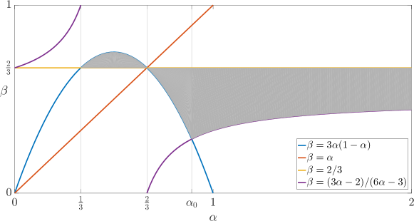
Figure 1: The gray area represents all $(\alpha,\beta)$ pairs which fulfill the conditions (15), i. e. for which the Butcher tableau (14) is non-negative [30].

The resulting MPRK43$(\alpha,\beta)$ method is determined by (13) using (14) and

$$p =3a_{21}(a_{31}+a_{32})b_{3}=\alpha\frac{2-3\alpha}{2(\beta-\alpha)}, q =a_{21}=\alpha,$$

$$\beta_{2} =\frac{1}{2a_{21}}=\frac{1}{2\alpha}, \beta_{1} =1-\beta_{2}=1-\frac{1}{2\alpha}.$$

2.2.2 MPRK43($\gamma$)

It was also proven in [30, Lemma 6] that all entries of the tableau

$$\begin{array}[]{c|ccc}0&&&\\ \frac{2}{3}&\frac{2}{3}&&\\ \frac{2}{3}&\frac{2}{3}-\frac{1}{4\gamma}&\frac{1}{4\gamma}&\\ \hline\cr&\frac{1}{4}&\frac{3}{4}-\gamma&\gamma\end{array}$$ (16)

are non-negative for $\frac{3}{8}\leq\gamma\leq\frac{3}{4}.$ Furthermore, in [48] it was proven that the resulting RK method is third-order accurate. The corresponding third-order MPRK scheme is denoted by MPRK43$(\gamma)$ and can be obtained from (13) by substituting (16) and

$$p =3a_{21}(a_{31}+a_{32})b_{3}=\frac{4}{3}\gamma, q =a_{21}=\frac{2}{3},$$

$$\beta_{2} =\frac{1}{2a_{21}}=\frac{3}{4}, \beta_{1} =1-\beta_{2}=\frac{1}{4}.$$

2.3 Embedded Methods of MPRK Schemes

It was proven in [29, 30] and generalized in [32, Lemma 5.4] that if the MPRK scheme is of order $k$, then the embedded method returning $\bm{\sigma}$ is of order $k-1$. In particular, in the case of MPRK22($\alpha$) the embedded method is first order and reads

$$y_{i}^{(1)}= \,y_{i}^{n},$$

$$y_{i}^{(2)}= \,y_{i}^{n}+\alpha\Delta t\sum_{j=1}^{N}\left(p_{ij}(\mathbf{y}^{(1)})\frac{y_{j}^{(2)}}{y_{j}^{n}}-d_{ij}(\mathbf{y}^{(1)})\frac{y_{i}^{(2)}}{y_{i}^{n}}\right),$$

$$\sigma_{i}= \,(y_{i}^{(2)})^{\frac{1}{\alpha}}(y_{i}^{n})^{1-\frac{1}{\alpha}}$$

for $i=1,\dotsc,N$. Similarly, the embedded second-order scheme for the two MPRK43 families is given by (13a)–(13d) with the respective parameters specified in the Subsections 2.2.1 and 2.2.2.

2.4 Preferable Members of MPRK Families

Since several families of MPRK methods exist [29, 30], a first challenge is to determine which member to choose. An intuitive way to disqualify certain members of the family is based on a stability investigation. However, as MPRK schemes do not belong to the class of general linear methods, a new approach was used in [38, 39] to investigate their stability properties. The resulting theory is based on the center manifold theorem for maps [49, 50] and was applied to second-order MPRK22($\alpha$) [39] and to third-order MPRK methods MPRK43($\alpha,\beta$) and MPRK43($\gamma$) in [41]. To that end, the linear problem

$$\mathbf{y}^{\prime}(t)=\mathbf{\Lambda}\mathbf{y}(t),\quad\mathbf{y}(0)=\mathbf{y}^{0}\in\mathbb{R}^{N}_{>0}$$ (17)

was considered, where $\mathbf{\Lambda}=(\lambda_{ij})_{i,j=1,\dotsc,N}\in\mathbb{R}^{N\times N}$ is a Metzler matrix, i. e. $\lambda_{ij}\geq 0$ for $i\neq j$, which additionally satisfies $\sum_{i=1}^{N}\lambda_{ij}=0$ for $j=1,\dotsc,N$. These two properties guarantee the positivity and conservativity of (17), see [39]. In particular, the aim of the analysis was to derive restrictions for the time step size guaranteeing that Lyapunov stable steady states of (17) are Lyapunov stable fixed points of the numerical scheme, see [38] for the details. Moreover, in the case of stable fixed points, the iterates of the MPRK method are proved to locally converge towards the correct steady state solution. The stability properties as well as the local convergence could be observed in numerical experiments [39, 41]. Indeed, it turned out that MPRK22$(\alpha$) and MPRK43$(\gamma$) are stable in this sense for all parameter choices [39, 41]. Still, the work [43] favors $\alpha=1$ for the MPRK22$(\alpha$) scheme for reasons of oscillatory behavior and the existence of spurious steady steady states. In the case of MPRK43$(\gamma$) we restrict to $\gamma=0.563$, since the corresponding scheme has the largest $\Delta t$ bound while fulfilling the necessary condition for avoiding oscillatory behavior, see [44].

Also, applying the stability analysis from [41] to the pairs $(\alpha,\beta)$ used so far [30], the pair $(\alpha,\beta)=(0.5,0.75)$ is associated with the largest stability domain.

As a result of that numerical analysis, we will consider MPRK43($\alpha,\beta$) with $\alpha=0.5$ and $\beta=0.75$ in the following.

Altogether, we will consider in this work the schemes MPRK22$(1)$, MPRK43$(0.5,0.75)$, and MPRK43$(0.563)$.

3 The Controller

Given an absolute tolerance atol and a relative tolerance rtol, we define the weighted error estimate

$$w_{n+1}=\left(\frac{1}{N}\sum_{i=1}^{N}\left(\frac{y_{i}^{n+1}-\sigma_{i}}{\mbox{{atol}}+\mbox{{rtol}}\max\{\lvert y_{i}^{n+1}\rvert,\lvert\sigma_{i}\rvert\}}\right)^{2}\right)^{\frac{1}{2}},$$ (18)

where $\mathbf{y}^{n+1}=(y_{1}^{n+1},\dotsc,y_{N}^{n+1})^{T}$ is the numerical approximation at time $t_{n+1}$ and $\bm{\sigma}$ the corresponding output of the embedded $(k-1)$th order method as mentioned in Section 2.3. Next, we set

$$\epsilon_{n+1}=\frac{1}{\max\{\mbox{{eps}},w_{n+1}\}},$$ (19)

where eps denotes machine precision. The proportional-integral-derivative (PID) controller with free parameters

$$(\beta_{1},\beta_{2},\beta_{3})\in[0.1,1]\times[-0.4,-0.05]\times[0,0.1]$$

is then given by

$$\Delta t_{n+1}=\epsilon_{n+1}^{\frac{\beta_{1}}{k}}\epsilon_{n}^{\frac{\beta_{2}}{k}}\epsilon_{n-1}^{\frac{\beta_{3}}{k}}\Delta t_{n},$$

with $\epsilon_{0}=\epsilon_{-1}=1$. Here, $k$ denotes the order of the MPRK method. Furthermore, for solving stiff problems, we extend the controller using ideas from digital signal processing [9]. Thus, we use the additional factor $\left(\frac{\Delta t_{n}}{\Delta t_{n-1}}\right)^{-\alpha_{2}}$ with $\alpha_{2}\in[1/6,1/2]$, so that

$$\Delta t_{n+1}=\epsilon_{n+1}^{\frac{\beta_{1}}{k}}\epsilon_{n}^{\frac{\beta_{2}}{k}}\epsilon_{n-1}^{\frac{\beta_{3}}{k}}\left(\frac{\Delta t_{n}}{\Delta t_{n-1}}\right)^{-\alpha_{2}}\Delta t_{n}.$$

Also, it is common to limit the new time step by a bounded function. Altogether, we use the DSP controller

$$\Delta t_{n+1}=\left(1+\kappa_{2}\arctan\left(\frac{\epsilon_{n+1}^{\frac{\beta_{1}}{k}}\epsilon_{n}^{\frac{\beta_{2}}{k}}\epsilon_{n-1}^{\frac{\beta_{3}}{k}}\left(\frac{\Delta t_{n}}{\Delta t_{n-1}}\right)^{-\alpha_{2}}-1}{\kappa_{2}}\right)\right)\Delta t_{n}$$ (20)

with $\kappa_{2}\in\{1,2\}$ as suggested in [7], i. e.

$$(\beta_{1},\beta_{2},\beta_{3},\alpha_{2},\kappa_{2})\in[0.1,1]\times[-0.4,-0.05]\times[0,0.1]\times[1/6,1/2]\times\{1,2\}.$$

We also note that if the coefficient of $\Delta t_{n}$ is smaller than a safety value of $s_{f}\coloneqq 0.81$, we reject the current step since it led to a small coefficient of $\Delta t_{n}$ and use $\Delta t_{n+1}$ to recalculate it.

As we want to test the reliability of the cost function, we rather consider the larger domain

$$D\coloneqq[-5,5]\times[-3,3]\times[-2,2]\times[-3,3]\times\{1,2,3,4\}$$ (21)

including further controllers from [9, 10, 51, 11, 12]. To give an insight on the effect of the limiter, we plot the function

$$L_{\kappa_{2}}(x)=1+\kappa_{2}\arctan\left(\frac{x-1}{\kappa_{2}}\right)$$

for the mentioned values of $\kappa_{2}$ in Figure 2.

0.5

Figure 2: Plots of $s_{f}=0.81$ and $L_{\kappa_{2}}(x)=1+\kappa_{2}\arctan\left(\frac{x-1}{\kappa_{2}}\right)$ for $\kappa_{2}\in\{1,2,3,4\}$ with logarithmic $x$-axis.

As it can be observed from Figure 2, $L_{\kappa_{2}}$ is steeper and allows larger changes in the step size for increasingly values of $\kappa_{2}\in\{1,2,3,4\}$ while maintaining approximately the same threshold for rejecting a step, meaning the intersection points of $L_{\kappa_{2}}$ with $s_{f}=0.81$ all lie in the interval $[0.8076,0.81]$.

3.1 Criteria for Good Controllers

Designing good step size controllers is difficult in general. If we consider a fixed combination of main method and embedded method, we could sample the space of all possible controller parameters. Then, for each problem and each tolerance, we could find an “optimal” controller resulting in the least error with the lowest amount of computational work. However, we do not want to make the controller dependent on the ODE to be integrated or the tolerance chosen by the user. Thus, we need to find controllers that perform well for a range of problems and tolerances.

The classical (deadbeat) I controller [2, Section II.4] is derived for the asymptotic regime of small time step sizes and can be argued to be optimal there. However, practical applications require controllers that also work well for bigger tolerances. For explicit Runge–Kutta methods and mildly stiff problems, step size control stability is important [52, 53] and led to the development of more advanced controllers such as PI controllers [4]. However, this theory of step size control stability is based on a linear stability analysis not applicable to MPRK methods. Moreover, it only gives necessary bounds on the controller parameters and still requires further tools to derive efficient controllers. See also [13, 54] for some recent studies in the context of computational fluid dynamics.

Further criteria for good controllers are discussed in [7]. In particular, we would like to achieve computational stability, i.e., a continuous dependence of the computed results on the given parameters. An important aspect for computational stability is to avoid discontinuous effects in the controller and already imposed by the form of the DSP controller (20). Furthermore, we would like to achieve tolerance convergence, i.e., to get better results when decreasing the tolerance (up to restrictions imposed by machine accuracy). Finally, a good controller should be able to achieve an error imposed by a given tolerance with as little work as possible. Here, we mainly measure the work by the number of accepted and rejected steps (proportional to the number of function evaluations and linear system solves for MPRK methods).

4 Methodology

We apply the MPRK schemes introduced in Section 2, and further specified in Section 2.4, to several training problems which we will describe in Section A of the appendix. We choose $\mbox{{atol}}=\mbox{{rtol}}\eqqcolon\mbox{{tol}}$ in (18) and consider values

$$\mbox{{tol}}\in\mbox{{TOL}}\coloneqq\{10^{-j}\mid j=1,\dotsc,8\}.$$ (22)

We formally evaluate the numerical solution $\mathbf{y}_{\mathrm{num}}(t)$ for the times $t_{1},t_{2},\dotsc,t_{K}$. We measure the number of successful and rejected steps at time $t_{n}$ denoted by $S_{n}$ and $R_{n}$, respectively. Thus, $S_{K}$ and $R_{K}$ represent the number of successful and rejected steps at the end of the calculations. Moreover, we use the trapezoidal rule to approximate the relative $L_{2}$ error by introducing

$$\mbox{{L2err\_rel}}(\mathbf{t},\mathbf{Y},\mathbf{y}_{\textrm{ref}})\coloneqq\left(\frac{\sum_{k=0}^{K-1}\frac{\Delta t_{k+1}}{2}\left(\lVert\mathbf{y}_{\textrm{ref}}(t_{k})-\mathbf{y}^{k}\rVert_{2}^{2}+\lVert\mathbf{y}_{\textrm{ref}}(t_{k+1})-\mathbf{y}^{k+1}\rVert_{2}^{2}\right)}{\sum_{k=0}^{K-1}\frac{\Delta t_{k+1}}{2}\left(\lVert\mathbf{y}_{\textrm{ref}}(t_{k})\rVert_{2}^{2}+\lVert\mathbf{y}_{\textrm{ref}}(t_{k+1})\rVert_{2}^{2}\right)}\right)^{\frac{1}{2}},$$ (23)

where $\mathbf{Y}=\left(\mathbf{y}^{0}\rotatebox[origin={c}]{90.0}{$\dabar@\dabar@\dabar@$}\dotsc\rotatebox[origin={c}]{90.0}{$\dabar@\dabar@\dabar@$}\mathbf{y}^{K}\right)$, $\mathbf{t}=(t_{0},\dotsc,t_{K})^{T}$, and $\Delta t_{k+1}=t_{k+1}-t_{k}$. Then the trapezoidal rule yields

$$\left(\frac{\int_{t_{0}}^{t_{K}}\lVert\mathbf{y}_{\textrm{ref}}(t)-\mathbf{y}_{\mathrm{num}}(t)\rVert_{2}^{2}\mathrm{d}t}{\int_{t_{0}}^{t_{K}}\lVert\mathbf{y}_{\textrm{ref}}(t)\rVert_{2}^{2}\mathrm{d}t}\right)^{\frac{1}{2}}=\mbox{{L2err\_rel}}(\mathbf{t},\mathbf{Y},\mathbf{y}_{\textrm{ref}})+\mathcal{O}\left(\left(\max_{k=0,\dotsc,K-1}\Delta t_{k+1}\right)^{3}\right)$$

for smooth enough integral kernels. If no analytical solution is available, a reference solution will be computed using the built-in function ode15s in Matlab R2023a [55, 56] together with the inputs AbsTol = 1e-13 and RelTol = 1e-13 for the absolute and relative tolerances.

A first task is to find abortion criteria to reduce the computational cost. To that end, we ran preliminary experiments, which suggest that any of the MPRK methods equipped with standard controllers do not require more than $10^{6}$ total steps to solve any of the test problems (reviewed in Section A in the appendix). As a result of this, the calculations are aborted if $S_{\max}\coloneqq 10^{6}$ steps are successful or if $R_{\max}\coloneqq 10^{4}$ steps were rejected or $R_{n}\geq\frac{S_{\max}}{R_{\max}}(S_{n}+1)=10^{2}(S_{n}+1)$ holds at some point during the calculations. With that in mind, it might be possible that $t_{K}\neq t_{\mathrm{end}}$ or $K=0$. In the latter case, we divide by $0$ in (23), which is why we introduce

$$\mbox{{err}}(\mathbf{t},\mathbf{Y},\mathbf{y}_{\textrm{ref}})\coloneqq\begin{cases}\mbox{{L2err\_rel}}(\mathbf{t},\mathbf{Y},\mathbf{y}_{\textrm{ref}}),&K>0,\\ \mbox{{NaN}},&K=0.\end{cases}$$ (24)

We then search for the optimal parameters of the time step controller introduced in Section 3 by means of minimizing the following cost function.

Given a parameter $s>0$ (see Remark 3 below for its influence), we introduce a cost function

$$C_{s}\colon D \to\mathbb{R}^{+},$$

$$\mathbf{x}\coloneqq(\beta_{1},\beta_{2},\beta_{3},\alpha_{2},\kappa_{2}) \mapsto C_{s}(\mathbf{x}),$$

where the domain $D$ is specified in (21). For a given set T of test problems and a $k$th order method we propose the cost function $C_{s}$ given by

$$C^{\ast}_{s}(\mathbf{x})=\sum_{\text{test}\in\text{T}}\psi\left(\sum_{\mbox{{tol}}\in\mbox{{TOL}}}(C_{\text{Step}}(\text{test},\mbox{{tol}},\mathbf{x})+C_{\text{tol},s}(\text{test},\mbox{{tol}},\mathbf{x}))\right),$$ (25)

where $\psi(x)=\left(\arctan\bigl{(}\frac{x}{100}\bigr{)}\right)^{2}$ and

$$C_{\text{Step}}(\text{test},\mbox{{tol}},\mathbf{x})= k\cdot\ln\Bigl{(}S_{K}^{\ast}(\text{test},\mbox{{tol}},\mathbf{x})+R_{K}^{\ast}(\text{test},\mbox{{tol}},\mathbf{x})\Bigr{)}$$ (26)

$$+\ln\left(\frac{\mbox{{err}}(\mbox{{tol}},\text{test},\mathbf{x})}{\mbox{{tol}}}\right),$$

$$C_{\text{tol},s}(\text{test},\mbox{{tol}},\mathbf{x})= \max\left(0,\ln\left(\frac{\mbox{{err}}(\mbox{{tol}},\text{test},\mathbf{x})}{s\cdot\mbox{{tol}}}\right)\right).$$

Here, the superscript asterisk indicates that the value of the related function is replaced by a penalty value, if the corresponding calculation was aborted. The particular penalty values and some properties of the cost function are summarized in the following remark.

Remark 3.

Let us start discussing $C_{\text{Step}}$ by noting that in logarithmic scale, the slope between two consecutive points in the work-precision (WP) diagram equals $-k$ as $\Delta t\to 0$. Hence, $C_{\text{Step}}$ is such that any point on that straight line corresponds to the same cost, and everything below is cheaper.

However, this way it might happen that all points for the different tolerances are clustered in the upper left corner of the WP diagram. To punish this behavior, we also add $C_{\text{tol},s}$, which returns $0$ if $\emph{\mbox{{err}}}(\emph{\mbox{{tol}}},\text{test},\mathbf{x})\leq s\cdot\emph{\mbox{{tol}}}$. A sketch is given in Figure 3, where all points on the black line will be associated with the same cost. However, if the error exceeds $s\cdot\mbox{{\text{tol}}}$, the corresponding point lies on the red line and will yield higher costs. If we now add further lines for different tolerances into Figure 3, we see that the presence of the red segments ensures that clustered points are expensive.

Figure 3: Sketch of a WP diagram of a $k$th order method (in logarithmic scale).

In particular, assume that $\emph{\mbox{{err}}}(\emph{\mbox{{tol}}},\text{test},\mathbf{x})=10^{m}s\cdot\emph{\mbox{{tol}}}$ for some $m\in\mathbb{R}^{+}$. Then we find $C_{\text{tol},s}=m\ln(10)$, which means that exceeding a given tolerance by a factor of $10^{m}s$ will be punished proportionally to the exponent $m$.

Additionally, we have the following penalty values and conditions.

• If the calculation is aborted because of $S_{K}=S_{\max}$ or $R_{K}=R_{\max}$ we punish this by setting

  $$S^{\ast}=10\max\{S_{\max},R_{\max}\}\quad\text{ or }\quad R^{\ast}=10\max\{S_{\max},R_{\max}\},$$

  respectively.

• If $\Delta t_{n}<10^{-100}$ at some point, the calculation is aborted and we set

  $$S^{\ast}=10\max\{S_{\max},R_{\max}\}.$$

• If the slope of the straight line through two consecutive points in the WP diagram does not lie in the interval $(-\infty,-0.7)$, the DSP parameter combination is disqualified. An exception is the first slope in the WP diagram, which we only require to lie in the interval $(-\infty,-0.35)$. This approach is based on the fact that the slope should tend to $-k$ as $\Delta t\to 0$. The disqualification is done in our case by canceling the calculations and adding $M=10$ to the current value of the cost function $C_{s}$, which represents the value $C_{s}^{\ast}$. The penalty $M=10$ is a reasonable choice since we will consider four test problems, eight different tolerances, and methods of order at most three, so that

  $$\sum_{\mbox{{\text{tol}}}\in\mbox{{TOL}}}(C_{\text{Step}}(\text{test},\mbox{{\text{tol}}},\mathbf{x})+C_{\text{tol},s}(\text{test},\mbox{{\text{tol}}},\mathbf{x})) \leq 8\cdot(3\ln(20S_{\max})+20\ln(10))$$

  $$\leq 8\cdot(3\cdot 7\ln(20)+60)<10^{3}$$

  for any controller satisfying $\emph{\mbox{{err}}}(\emph{\mbox{{tol}}},\text{test},\mathbf{x})\leq 10^{10}s\cdot\emph{\mbox{{tol}}}$. In view of the transformation $\psi$, see Figure 4 for a plot of the graph, we thus observe that for each test, we obtain a value between $0$ and $2.5$ justifying the penalty addend $M=4\cdot 2.5$. With this transformation we make sure that a single test problem is not dominating the remaining, for instance due to a large value of $C_{\text{tol},s}$.

0.5

Figure 4: Plot of $\psi(x)=\left(\arctan\left(\frac{x}{100}\right)\right)^{2}$.

Remark 4.

The last ingredient disqualifying points with a wrong slope has to be adapted for methods with reduced stability properties such as explicit RK methods. Indeed, good controllers typically lead to a clustering of points in a work-precision diagram as observed for example in [57].

The minimum of the cost function $C_{s}$ is searched using the Bayesian optimization function bayesopt in Matlab [55] with $500$ iterations and the input arguments ’IsObjectiveDeterministic’ set to true as well as ’AcquisitionFunctionName’ set to ’expected-improvement-per-second-plus’ for a somewhat balanced trade off between exploration and exploitation, followed by a run with another $500$ iterations using the ’AcquisitionFunctionName’ set to ’probability-of-improvement’ enhancing the local search. Since we validate the results by means of plotting the WP diagram, the value $s=1$ is a natural choice here, meaning that there is no safety gap between tol and $s\cdot\mbox{{\text{tol}}}$ in Figure 3.

5 Controller Parameters

As described in Section 4, we use Bayesian optimization to determine customized parameters for the time step controller reviewed in Section 3.

We first focus on the performance of the standard parameters from [4, 5, 6, 7, 8, 9, 10, 11, 12] of the form (20), see Figure 6, 7, and 8. The parameter $(\tfrac{1}{6},-\tfrac{1}{3},0,0,1)$ [12] is by far the worst followed by $(\tfrac{1}{18},\tfrac{1}{9},\tfrac{1}{18},0,1)\approx(0.056,0.111,0.056,0,1)$ [9]. Furthermore, while the remaining controllers are somewhat similar in performance for the second-order scheme, the difference becomes clear for the third-order methods when solving PR4 and NPZD problem. With that, the overall best controller seems to be $p_{1}=(2,-1,0,-1,1)$ [9]. However, the second best is harder to read off from the images as the points are close to each other. Because of PR4, one might be tempted to declare the simple I controller $(1,0,0,0,1)$ as the second place; however, zooming into HIRES for MPRK22($1$) in Figure 5, we see that the performance for large tolerances is not good. Rather, the parameters $p_{2}=(0.7,-0.4,0,0,1)$ and $p_{3}=(0.6,-0.2,0,0,1)$ seem to be promising candidates.

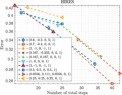
Figure 5: WP diagram for the HIRES problem using MPRK22(1) with several standard controllers and tolerance set $\{10^{-1},10^{-2}\}$.

A first test of our cost function is to see its ranking for the standard parameters. Indeed, $p_{1}$, $p_{2}$ and $p_{3}$ are the only controllers that have a cost smaller than $M=10$ and we find $C_{1}(p_{1})<\min\{C_{1}(p_{2}),C_{1}(p_{3})\}$, see Table 1. The remaining parameters did not perform well for large tolerances. However, the previously mentioned I controller performed well for the third-order methods which is in accordance with what we see in the Figures 6, 7 and 8 and Table 1.

Table 1: Costs of standard parameters using the cost function $C_{1}$.

Controller	MPRK22(1)	MPRK43I(0.5,0.75)	MPRK43II(0.563)
$(0.6,-0.2,0,0,1)$	3.7476	4.3530	4.4685
$(0.7,-0.4,0,0,1)$	3.7575	4.3572	4.4739
$(\tfrac{1}{6},-\tfrac{1}{3},0,0,1)$	11.8635	12.0161	12.0170
$(\tfrac{1}{6},\tfrac{1}{6},0,0,1)$	13.0422	13.5380	13.6471
$(1,0,0,0,1)$	10.0472	4.3077	4.4192
$(2,-1,0,-1,1)$	3.7062	4.2991	4.4115
$(0.5,0.5,0,0.5,1)$	10.0476	10.0673	12.2867
$(0.056,0.111,0.056,0,1)$	12.4297	12.8928	13.0054
$(0.25,0.25,0.25,0,1)$	10.0487	13.5249	12.2906

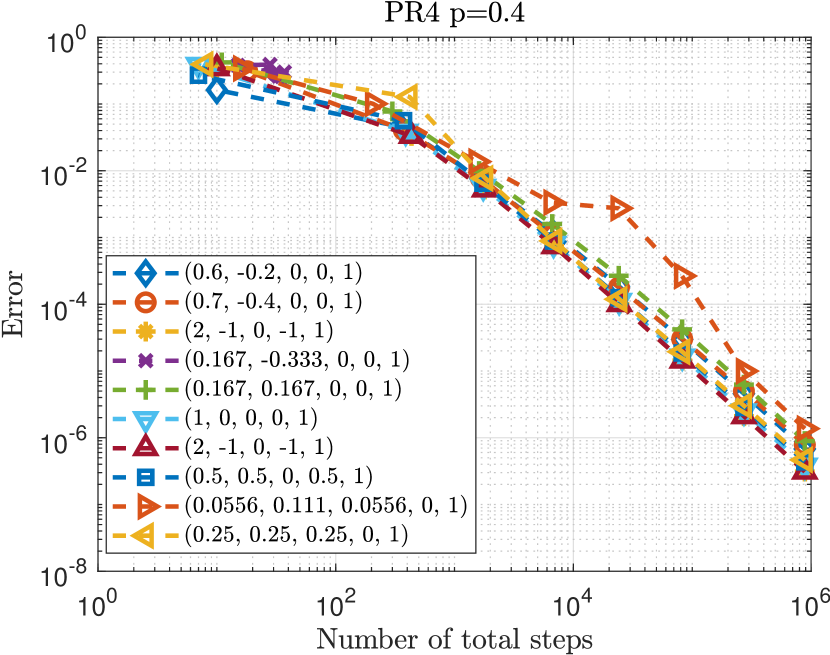
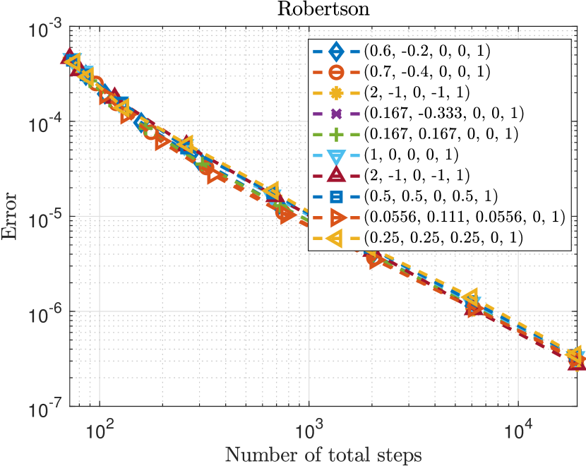
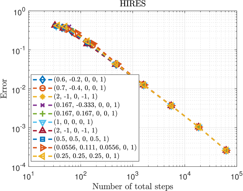
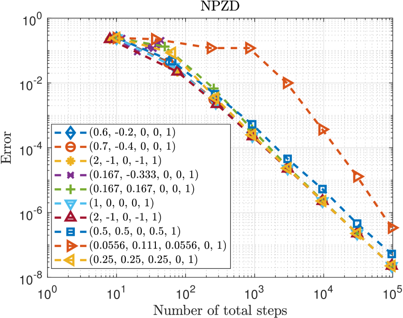
Figure 6: WP diagram for the test problems from Section A using MPRK22(1) with several standard controllers and tolerance set TOL from (22).

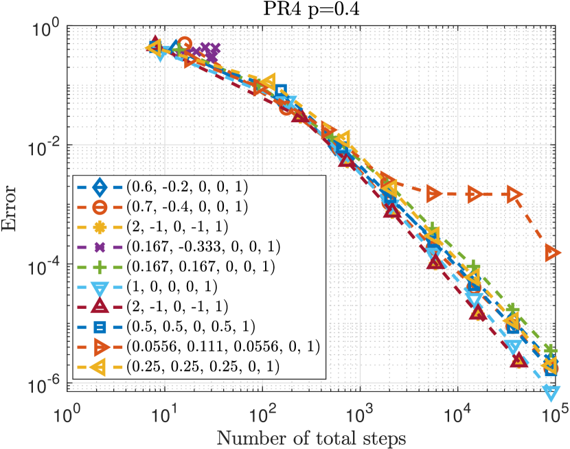
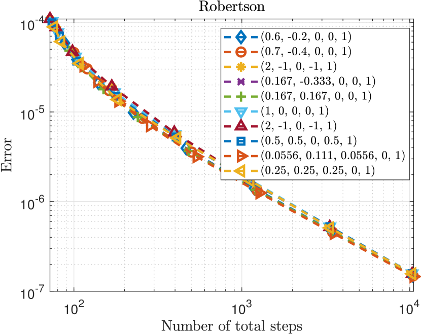
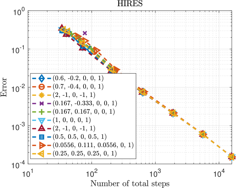
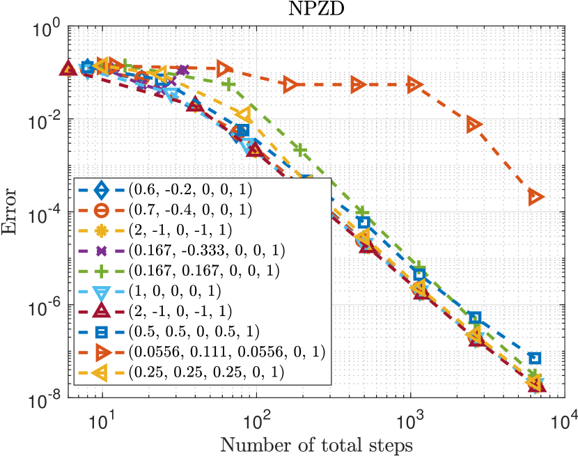
Figure 7: WP diagram for the test problems from Section A using MPRK43(0.5,0.75) with several standard controllers and tolerance set TOL from (22).

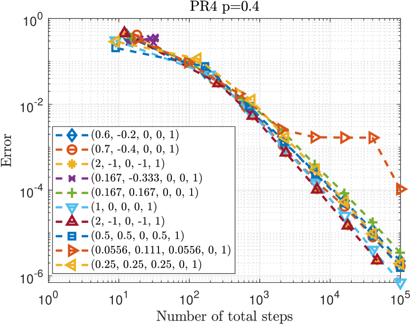
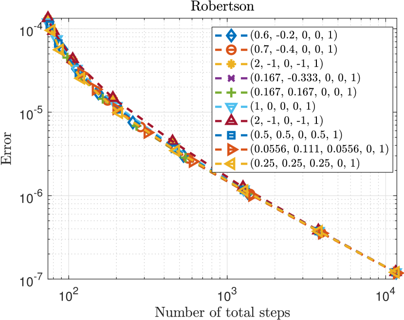
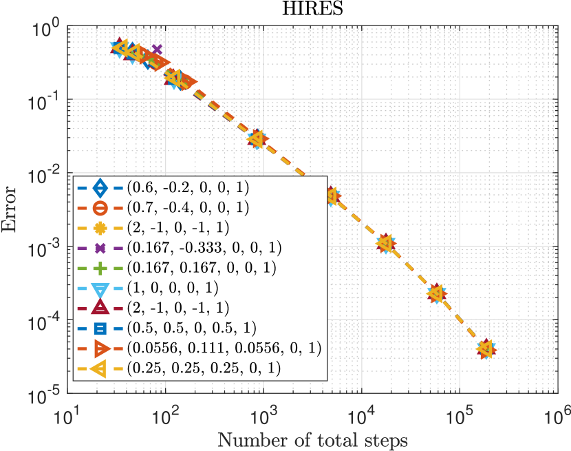
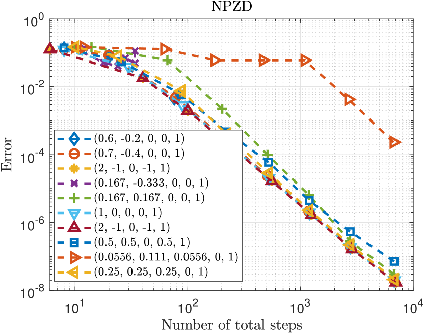
Figure 8: WP diagram for the test problems from Section A using MPRK43(0.563) with several standard controllers and tolerance set TOL from (22).

As a next step, we run our experiments using the cost function $C_{1}$ introduced in Section 4. The resulting customized parameters are summarized for the three schemes under consideration in Table 2. Already after 1000 total iterations within the Bayesian optimization we thus obtain parameters with similar if not even cheaper costs than those of the standard controllers.

Table 2: Customized parameters and cost $C_{1}$ after 1000 iterations total.

Method	$\beta_{1}$	$\beta_{2}$	$\beta_{3}$	$\alpha_{2}$	$\kappa_{2}$	$C_{1}$
MPRK22(1)	1.3651	0.12708	-0.57219	-0.37702	2	3.7086
MPRK43I(0.5,0.75)	1.1786	-0.47694	-0.027401	-0.71155	4	4.2596
MPRK43II(0.563)	1.2119	0.023048	-0.12786	-0.56604	2	4.3942

Now, since we most likely did not find the optimal parameters with this iterative approach, it is reasonable to check if any of the optimized parameters listed in Table 2 might lead do a decreased cost also for the other methods. Indeed, a direct comparison reveals that the parameter

$$(\beta_{1},\beta_{2},\beta_{3},\alpha_{2},\kappa_{2})=(1.1786,-0.47694,-0.027401,-0.71155,4)$$

is the overall cheapest with associated costs $3.7002$ and $4.3810$ for MPRK22(1) and MPRK43(0.563), respectively. As a result of this observation we are tempted to increase the total number of steps resulting in Table 3.

Table 3: Overall cheapest parameters and cost $C_{1}$ after 2000 iterations total.

Method	$\beta_{1}$	$\beta_{2}$	$\beta_{3}$	$\alpha_{2}$	$\kappa_{2}$	$C_{1}$
MPRK22(1)	1.951	-0.66961	-0.37409	-0.48842	2	3.6991
MPRK43(0.5,0.75)	1.7706	-0.27744	-0.37701	-0.95947	3	4.2572
MPRK43(0.563)	2.2556	-1.1991	-0.15024	-2.2167	2	4.3785

There, we found even better parameters with respect to our cost function. As before, we do a cross comparison of the costs of the controllers, which revealed no further improvement. This means that the parameters in Table 3 are the overall cheapest parameters found in this work.

Now let us compare the performances of the found parameters with those of the best fitting standard controllers $p_{1}$, $p_{2}$ and $p_{3}$. We start with the second-order MPRK scheme, see Figure 9. Here, it becomes evident that the new controller performs slightly better than the best standard controllers as, besides being highly accurate for small tolerances, it is also cheaper for the larger ones.

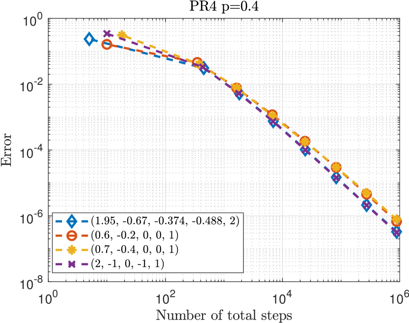
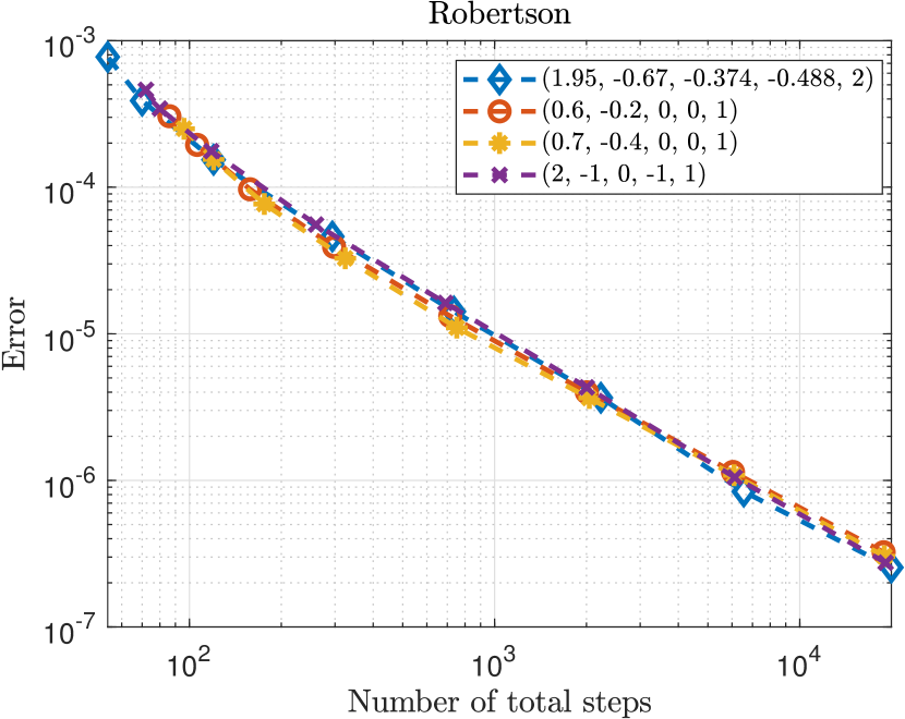
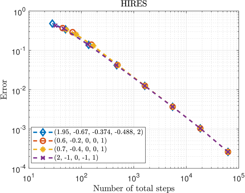
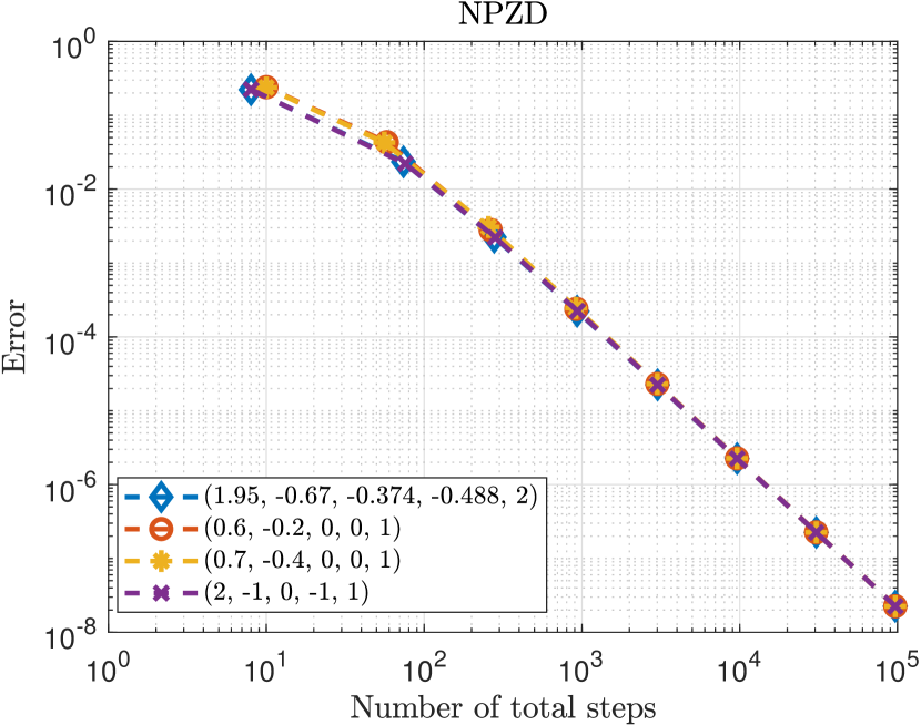
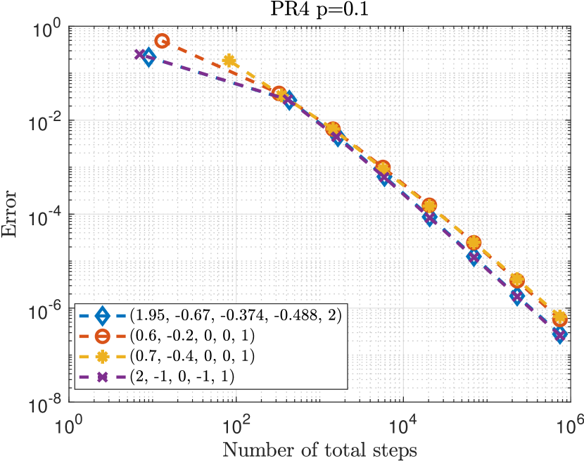
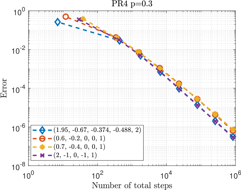
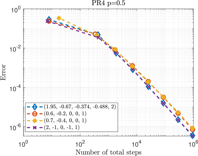
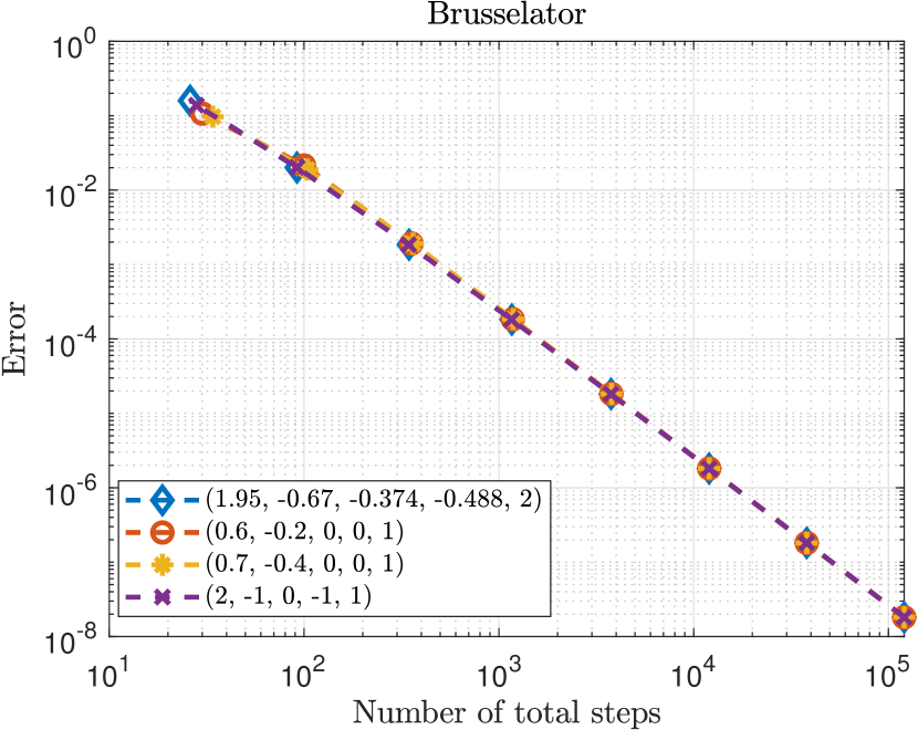
Figure 9: WP diagram of the problems from Section A and Section B using MPRK22(1) with the overall cheapest customized parameter and the best standard controllers $p_{1}$, $p_{2}$ and $p_{3}$.

This becomes even clearer when looking at the third-order schemes, see Figure 10 and Figure 11, respectively. Even though the found parameter is slightly less accurate for mid-ranged tolerances in the Robertson problem, the found controller performs clearly better at the largest and smallest tolerances. Also note that in the case of the Robertson problem the calculated error is below the given tolerance for $\mbox{{\text{tol}}}\in\{10^{-j}\mid j=1,\dotsc,5\}$, i. e. is meeting our requirements of a good controller.

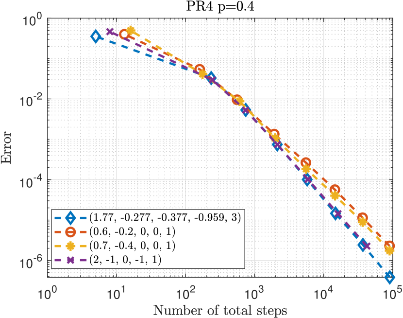
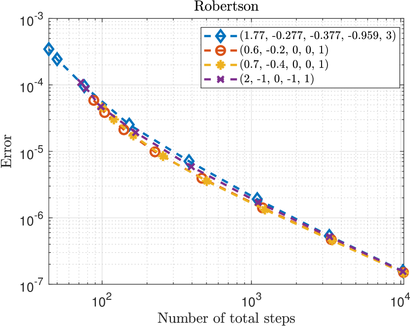
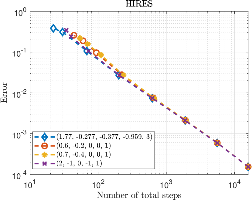
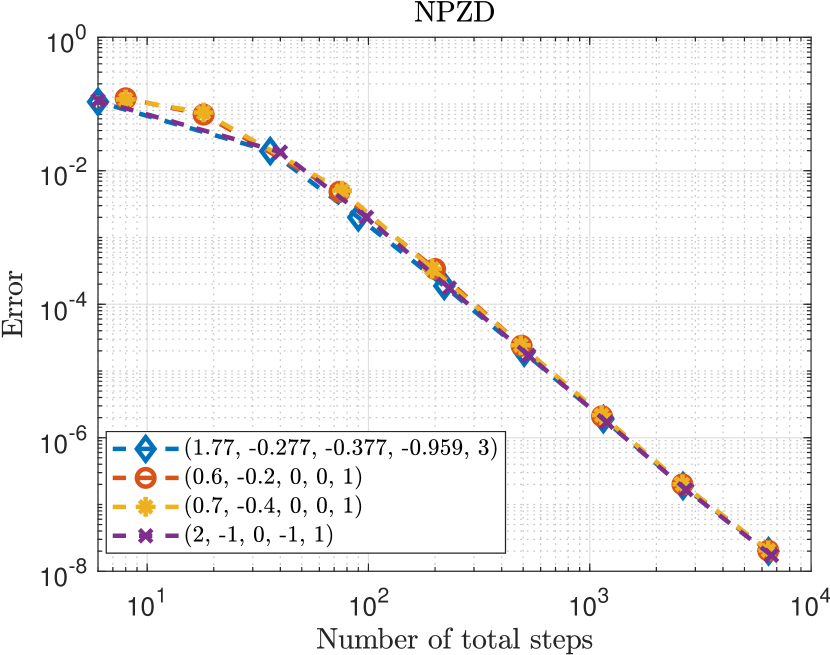
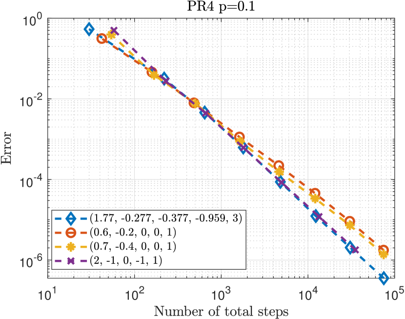
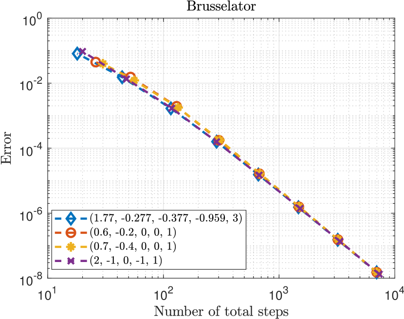
Figure 10: WP diagram of the problems from Section A and Section B using MPRK43(0.5,0.75) with the overall cheapest customized parameter and the best standard controllers $p_{1}$, $p_{2}$ and $p_{3}$.

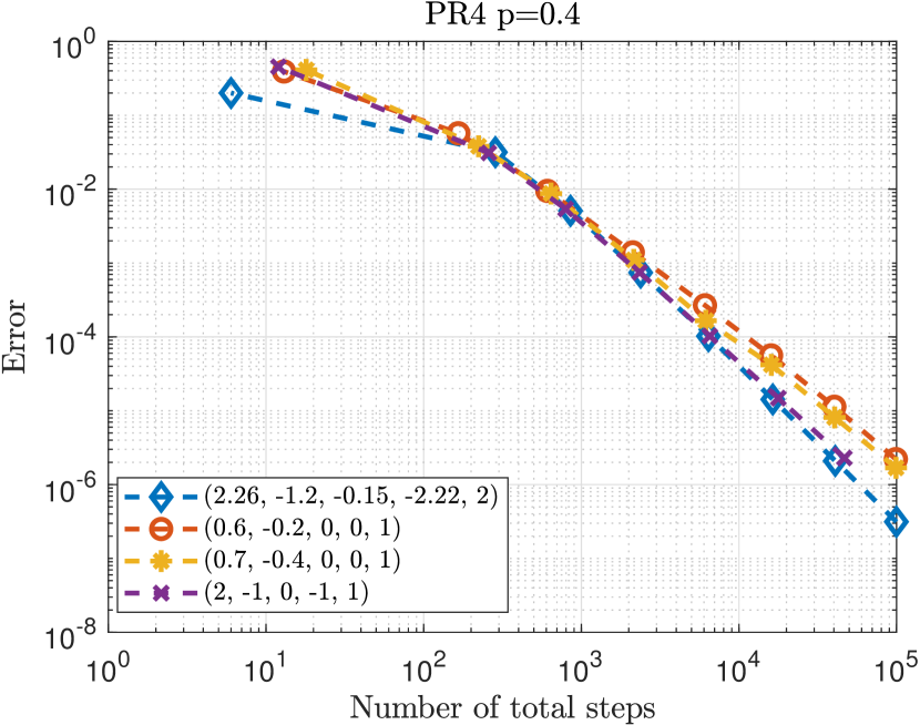
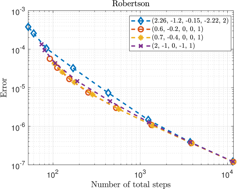
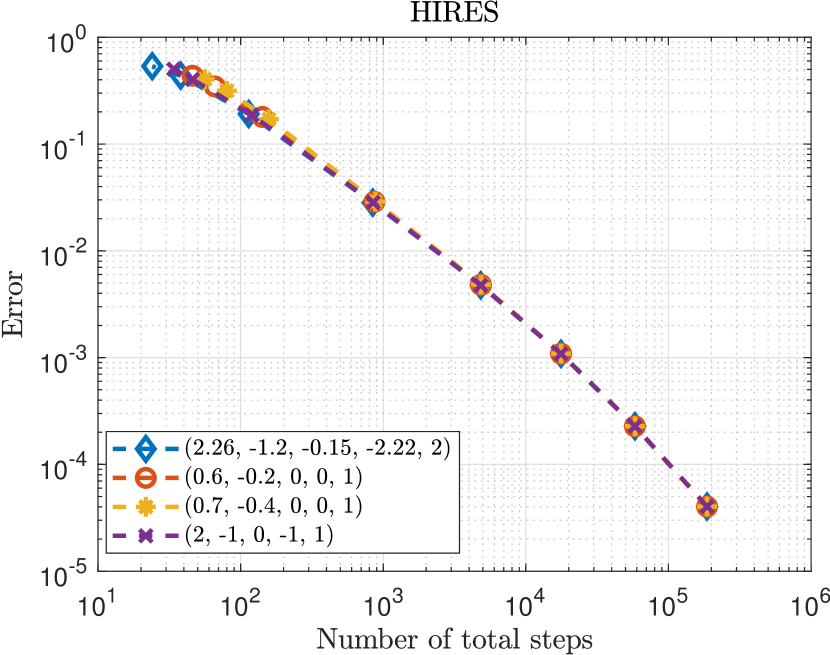
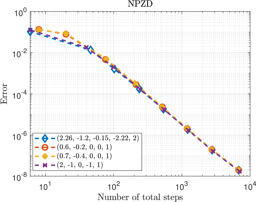
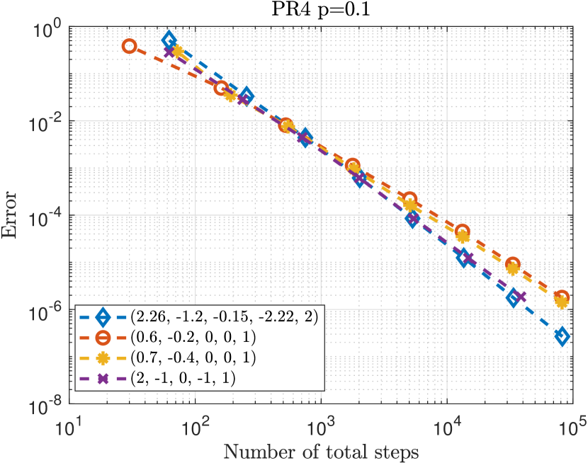
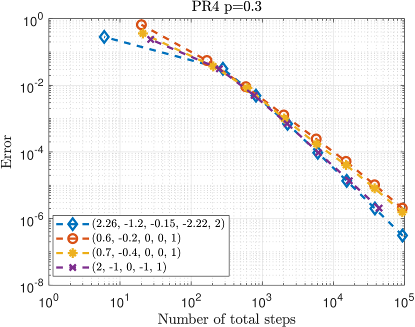
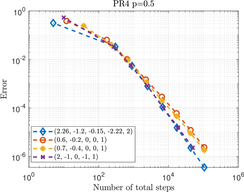
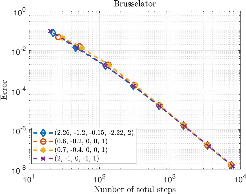
Figure 11: WP diagram of the problems from Section A and Section B using MPRK43(0.563) with the overall cheapest customized parameter and the best standard controllers $p_{1}$, $p_{2}$ and $p_{3}$.

5.1 Comparison with Adaptive Runge–Kutta Methods

We also compare the performance of MPRK methods with parameters presented in Table 3 with some standard time integration methods. A comparison of MPRK22(1) with constant step size to built-in solvers in Matlab for the NPZD problem (32) was already done in [21], where MPRK schemes were more efficient for coarser tolerances. In this work, we compare the MPRK schemes with adaptive time step control to the built-in solvers. In particular we compare the methods with the second-order, linearly implicit Rosenbrock scheme ode23s and the variable-order BDF method ode15s [56]. We compare the number of right-hand side (RHS) evaluations and the total runtime. For the latter we note that we use our proof of concept implementation which means that the comparison may be unfair given that these built-in functions are optimized in Matlab. The elapsed time is measured using the built-in functions tic and toc from Matlab. Furthermore, we averaged the elapsed time using five runs on a Lenovo notebook with an Intel i7-1065G7 processor and Matlab R2023b.

The results are depicted in Figure 12 for NPZD and Robertson problems. The results for the remaining test cases did not provide further insights and are thus omitted for the sake of a compact presentation.

In the case of NPZD, ode15s is the best for tolerances smaller than $10^{-3}$. However, this superior performance might be traced back to the variable order of the method and should be further investigated in the future. Nevertheless, for coarse tolerances ode15s is beaten by MPRK schemes, whereby the third-order methods perform better than MPRK22(1). Even more, the third-order MPRK schemes need fewer RHS evaluations than ode23s to reach the same error, which again might be explained by the order of the method. Still, MPRK22(1) can compete with ode23s for all given tolerances when it comes to the number of RHS evaluations.

In the case of the Robertson problem, ode23s performs better than MPRK for smaller tolerances. However, MPRK remain superior for coarser tolerances.

With regard to the computational time we note that the third-order MPRK schemes, even though being a proof of concept implementation, are faster than the built-in functions for most tolerances.

We also note that in all test cases, our cost function provided a controller which is computationally stable, whereas this cannot be said about the used built-in ODE solvers in Matlab R2023b. This can be particularly seen for ode15s applied to the Robertson problem with coarser tolerances, where the tolerance convergence can be observed only for stricter tolerances.

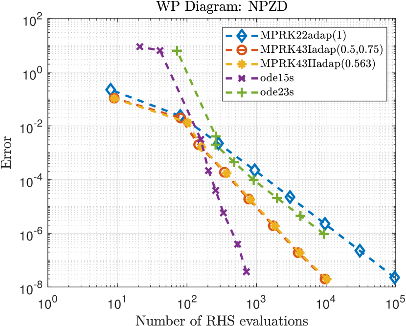
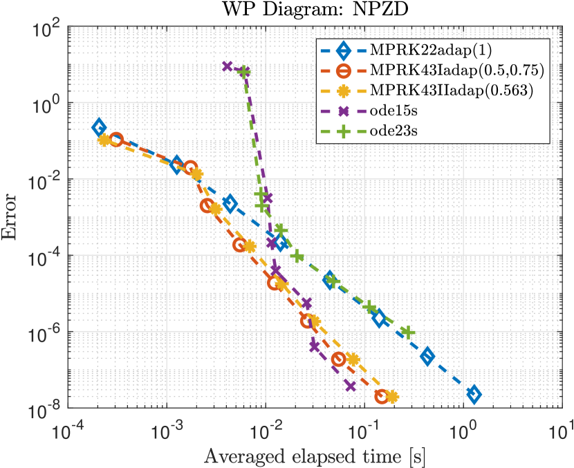
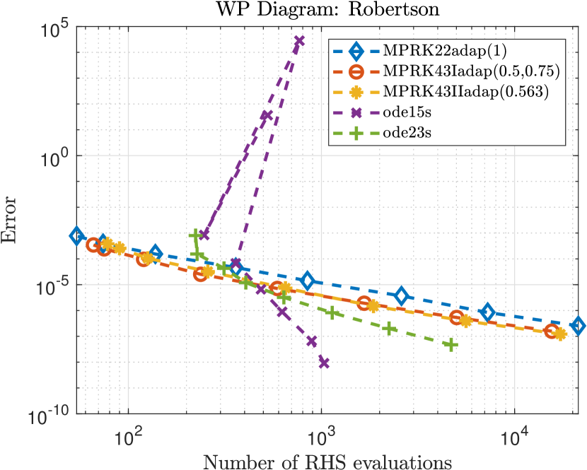
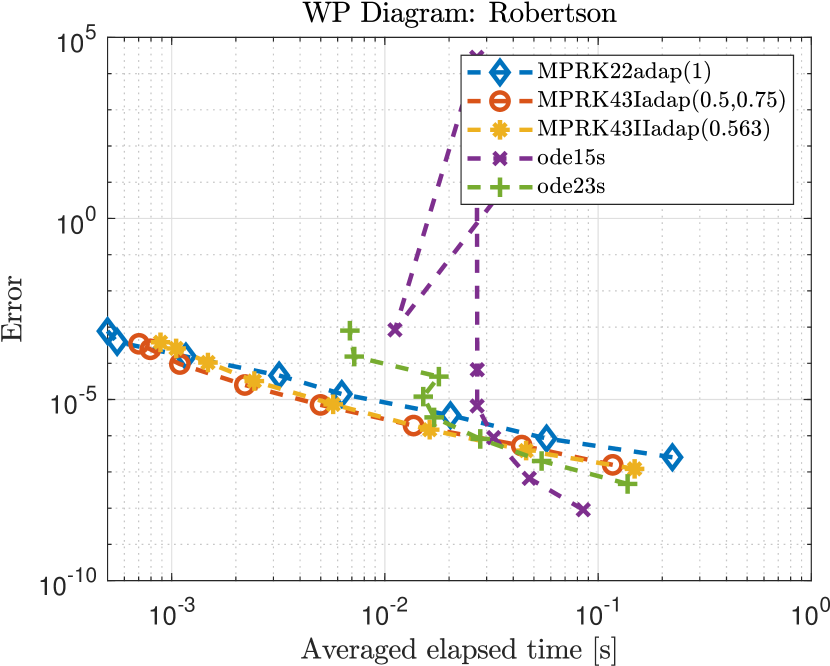
Figure 12: WP diagrams for the NPZD and Robertson problem (32) using the MPRK schemes with the DSP controllers from Table 3, and standard built-in Matlab solvers.

In general, it may be expected that MPRK schemes are performing better than Runge–Kutta methods for coarser tolerances and test problems whenever the time step restrictions for a given tolerance are dominated by the demand for positive approximations. One example is given by the NPZD problem where a method producing negative approximations is in danger to diverge. Hence, while MPRK schemes are guaranteed to produce positive approximations for every time step, no matter how big, the built-in solvers can achieve this goal only by means of a time step reduction yielding a larger number of steps, and thus, RHS evaluations. Now, if the given tolerance is getting smaller, the time step size restrictions for positivity are fulfilled by the requirement of producing more accurate approximations, and hence, the benefit of MPRK schemes is lost. Already because of this, we argue that MPRK schemes are worth considering whenever positivity of the numerical solution is interlinked with severe time step constraints. However, we discovered the same dominating behavior for all given test problems, which is why the reason for the better performance for coarser tolerances may lie elsewhere.

6 Summary and Conclusion

We have developed an approach to design time step size controllers using Bayesian optimization for modified Patankar–Runge–Kutta (MPRK) methods. The basic idea is to use a general ansatz of step size controllers from digital signal processing including PI and PID controllers. Then, we search for a relevant set of test problems and design an appropiate cost function used for the Bayesian optimization of the controller parameters. Finally, the resulting controllers are validated for another set of additional benchmarks.

The choice of test problems and the cost function is important to obtain good results. This approach is comparable in spirit to [13], where a numerical search based on well-chosen test problems was used in the context of designing adaptive time integration methods for compressible computational fluid dynamics. As described therein, the set of test problems needs to represent different regimes that can appear in practicar applications, i.e., the problems should have different characteristics such as stiffness properties. Focusing on MPRK methods, we have chosen several ordinary differential equations linked to chemical reactions and biological systems for this task. In contrast to [13], we have developed a cost function to be used in Bayesian optimization to obtain the parameters of the controllers. The design process of the cost function took several iterations and took into account desirable properties such as computational stability and tolerance convergence. The cost function (25) is developed specifically for schemes such as MPRK methods with good stability properties that are able to handle even some stiff problems well. If the same approach was used for other schemes such as explicit Runge–Kutta schemes, additional properties such as step size control stability for mildly stiff problems should be taken into account. The extension of our approach to cases like this is left for future work.

Finally, we have applied the optimization-based approach to three MPRK schemes proposed in the literature: the second-order method MPRK22$(1)$ [29] and the third-order methods MPRK43$(0.5,0.75)$ and MPRK43$(0.563)$ [30]. The optimized controllers for these methods are summarized in Table 3. A proof-of-concept implementation of the methods with the optimized controllers are already comparable to Matlab solvers such as ode23s for loose tolerances.

Along the way, we have also some new results on MPRK schemes that are interesting on their own. In particular, we have extended MPRK schemes to general time-dependent production-destruction-rest systems in Section 2, broadening the scope of applications of this class of methods.

Declarations

Funding The author T. Izgin gratefully acknowledges the financial support by the Deutsche Forschungsgemeinschaft (DFG) through the grant ME 1889/10-1 (DFG project number 466355003). H. Ranocha was supported by the Deutsche Forschungsgemeinschaft (DFG, German Research Foundation, project number 513301895) and the Daimler und Benz Stiftung (Daimler and Benz foundation, project number 32-10/22).

Conflict of interest The authors declare that they have no conflict of interest.

Availability of code, data, and materials The source code used in this study is based on a closed-source inhouse research code developed at the University of Kassel. The data generated for this study is available from the corresponding author upon reasonable request.

Authors’ contributions Conceptualization: Thomas Izgin, Hendrik Ranocha; Data curation: Thomas Izgin; Formal analysis and investigation: Thomas Izgin, Hendrik Ranocha; Software: Thomas Izgin; Visualization: Thomas Izgin; Writing - original draft preparation: Thomas Izgin, Hendrik Ranocha; Writing - review and editing: Thomas Izgin, Hendrik Ranocha.

Appendix

Appendix A Training Problems

In this section we present several test problems for deriving optimized DSP parameters by the methodology described in the previous section. Thereby, the controller together with the MPRK scheme is challenged to learn how to efficiently increase and decrease the step size in order to solve stiff problems.

Before proceeding, it is important to note that MPRK schemes need strictly positive initial data. Hence, zeros in the initial vector will be replaced by realmin which is around $10^{-308}$ for 64 bit floating point numbers used in the implementation.

A.1 Prothero & Robinson Problem

Introducing a $\mathcal{C}^{1}$-map $\mathbf{g}$, we consider

$$\mathbf{y}^{\prime}(t)=\mathbf{\Lambda}(\mathbf{y}(t)-\mathbf{g}(t))+\mathbf{g}^{\prime}(t),\quad\mathbf{y}(0)=\mathbf{y}^{0}\in\mathbb{R}^{N}_{>0}.$$ (27)

We want to note that choosing $\mathbf{\Lambda}\in\mathbb{R}^{N\times N}$ as a Metzler matrix satisfying $\bm{1}\in\ker(\mathbf{\Lambda}^{T})$ and $\mathbf{g}=\mathbf{0}$, this problem degenerates to (17). The problem (27) is related to the Prothero & Robinson problem introduced in [58].

If $\mathbf{g}$ is smooth with $\mathbf{g}(0)=\mathbf{y}(0)$, then $\mathbf{y}=\mathbf{g}$ is the unique solution to the initial value problem. Therefore, choosing positive initial data and $\mathbf{g}>\mathbf{0}$ guarantees the positivity of the solution of (27).

In what follows, we solve the problem (27) for $N=4$ using a matrix $\mathbf{\Lambda}_{\xi}\in\mathbb{R}^{4\times 4}$, whose spectrum runs over a vertical line in $\mathbb{C}^{-}$ as $\xi$ passes through the interval $[0,1]$. In particular,

$$\mathbf{\Lambda}_{\xi}=\begin{pmatrix}[r]-1&1-\xi&\xi&0\\ \xi&-1&0&1-\xi\\ 1-\xi&0&-1&\xi\\ 0&\xi&1-\xi&-1\end{pmatrix}$$

satisfies $\sigma(\mathbf{\Lambda}_{\xi})=\{0,-2,(2\xi-1)\mathrm{i}-1,(1-2\xi)\mathrm{i}-1\}$. Now according to [59], any eigenvalue $\lambda$ of a Metzler matrix $\mathbf{\Lambda}\in\mathbb{R}^{4\times 4}$ with $\operatorname{Re}(\lambda)=-1$ satisfies $\operatorname{Im}(\lambda)\in[-1,1]$, so that we cover all possible eigenvalues when choosing $\xi\in[0,1]$. Indeed, due to symmetry, we only need to consider $\xi\in[0,1/2]$. For the training we restrict to only one test case using $\xi=0.4$ in order to avoid an artificially large influence of this test problem on the cost function. However, we will use several values of $\xi$ for the validation of our results.

Next, we use

$$\mathbf{g}(t)=\begin{pmatrix}[r]2+0.3\sin(0.5\cos(0.5t)t)\\ 2+\sin(0.5\cos(0.5t)t)\\ 1-\sin(0.5\cos(0.5t)t)\\ 1-0.3\sin(0.5\cos(0.5t)t)\end{pmatrix}$$ (28)

and note that $g_{1}^{\prime}(t)=-g_{4}^{\prime}(t)$ and $g_{2}^{\prime}(t)=-g_{3}^{\prime}(t)$. The graph of $\mathbf{g}$, i. e. the solution of (27) can be seen in Figure 13. As one can observe, the time-dependent frequency results in an increasing amount of local maxima and minima of different magnitude.

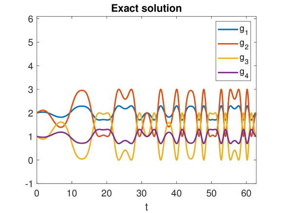
Figure 13: Graph of $\mathbf{g}$ from (28) over the time interval $[0,20\pi]$.

Finally, the corresponding problem (27) will be approximated over the interval $[0,20\pi]$ can be written as a PDS using $p_{ij}=d_{ji}$ and

$$p_{12}(\mathbf{y},t) =y_{2}, p_{13}(\mathbf{y},t) =g_{1}(t), p_{14}(\mathbf{y},t) =\xi(y_{3}+g_{2}(t))+\min(0,g^{\prime}_{1}(t)),$$ (29)

$$p_{21}(\mathbf{y},t) =g_{2}(t), p_{24}(\mathbf{y},t) =y_{4}, p_{23}(\mathbf{y},t) =\xi(g_{4}(t)+y_{1})+\min(0,g^{\prime}_{2}(t)),$$

$$p_{31}(\mathbf{y},t) =y_{1}, p_{34}(\mathbf{y},t) =g_{3}(t), p_{32}(\mathbf{y},t) =\xi(g_{1}(t)+y_{4})+\min(0,g^{\prime}_{3}(t)),$$

$$p_{42}(\mathbf{y},t) =g_{4}(t), p_{43}(\mathbf{y},t) =y_{3}, p_{41}(\mathbf{y},t) =\xi(y_{2}+g_{3}(t))+\min(0,g^{\prime}_{4}(t)).$$

In the following, we will refer to this problem as PR4 and use the initial time step size $\Delta t_{0}=1$.

A.2 Robertson’s Problem

The well-known Robertson problem is stiff [3, Section IV.1] and reads

$$y_{1}^{\prime}(t) =10^{4}y_{2}(t)y_{3}(t)-0.04y_{1}(t),$$ (30)

$$y_{2}^{\prime}(t) =0.04y_{1}(t)-10^{4}y_{2}(t)y_{3}(t)-3\cdot 10^{7}(y_{2}(t))^{2},$$

$$y_{3}^{\prime}(t) =3\cdot 10^{7}(y_{2}(t))^{2}.$$

We use the initial condition $\mathbf{y}=(1,0,0)^{T}$ and initial time step size $\Delta t_{0}=10^{-6}$. A reference solution to this problem for $t\in[0,10^{8}]$ is depicted in Figure 14, where $y_{2}$ is multiplied with $10^{4}$ for visualization purposes. Moreover, this problem is positive and conservative, i. e. $\mathbf{n}=(1,1,1)^{T}$ satisfies $\mathbf{n}^{T}\mathbf{y}(t)=\operatorname{const}$.

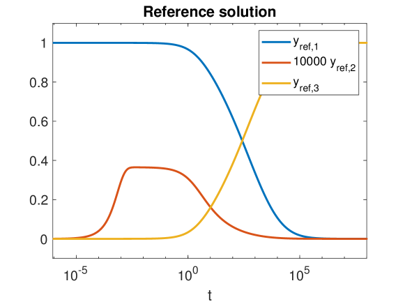
Figure 14: Reference solution of the Robertson problem (30) with logarithmic $t$-axis over the interval $[0,10^{8}]$.

A.3 HIRES Problem

The "High Irradiance RESponse" (HIRES) problem, see [60, 61, 3], takes the form

$$y_{1}^{\prime} =-1.71y_{1}+0.43y_{2}+8.32y_{3}+0.0007,$$ (31)

$$y_{2}^{\prime} =1.71y_{1}-8.75y_{2},$$

$$y_{3}^{\prime} =-10.03y_{3}+0.43y_{4}+0.035y_{5},$$

$$y_{4}^{\prime} =8.32y_{2}+1.71y_{3}-1.12y_{4},$$

$$y_{5}^{\prime} =-1.745y_{5}+0.43y_{6}+0.43y_{7},$$

$$y_{6}^{\prime} =-280y_{6}y_{8}+0.69y_{4}+1.71y_{5}-0.43y_{6}+0.69y_{7},$$

$$y_{7}^{\prime} =280y_{6}y_{8}-1.81y_{7},$$

$$y_{8}^{\prime} =-280y_{6}y_{8}+1.81y_{7}.$$

The nonzero entries of the initial vector are $y_{1}(0)=1$ and $y_{8}(0)=0.0057$. The system of ODEs can be written as a PDRS (3) with $\mathbf{r}^{p}(\mathbf{y})=(0.0007,0,0,0,0.43y_{7},0.69y_{7},0,0)^{T}$, $\mathbf{r}^{d}(\mathbf{y})=(0,0,0,0,0,280y_{6}y_{8},0,0)^{T}$ and

$$p_{12}(\mathbf{y}) =0.43y_{2}, p_{13}(\mathbf{y}) =8.32y_{3}, p_{21}(\mathbf{y}) =1.71y_{1},$$

$$p_{34}(\mathbf{y}) =0.43y_{4}, p_{35}(\mathbf{y}) =0.035y_{5}, p_{42}(\mathbf{y}) =8.32y_{2},$$

$$p_{43}(\mathbf{y}) =1.71y_{3}, p_{56}(\mathbf{y}) =0.43y_{6}, p_{64}(\mathbf{y}) =0.69y_{4},$$

$$p_{65}(\mathbf{y}) =1.71y_{5}, p_{78}(\mathbf{y}) =280y_{6}y_{8}, p_{87}(\mathbf{y}) =1.81y_{7}$$

being the non-vanishing production terms and $d_{ij}=p_{ji}$. The problem will be approximated on the interval $[0,321.8122]$ using the initial time step size $\Delta t_{0}=0.5\cdot 10^{-3}$, and a reference solution can be found in Figure 15.

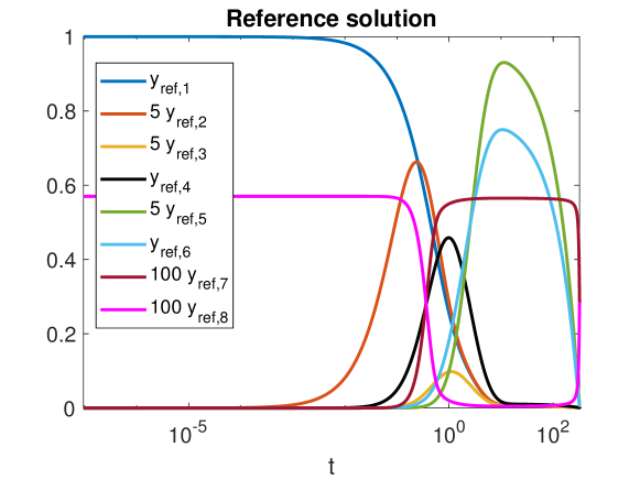
Figure 15: Reference solution of the HIRES problem (31) plotted over the time interval $[0,321.8122]$ with logarithmic $t$-axis. Thereby, the solution vector was scaled with $\operatorname{diag}(1,5,5,1,5,1,100,100)$.

This problem is interesting since it is a non-conservative PDS and the controller has to learn how to handle the different behavior of the solution on the respective time scales.

A.4 NPZD Problem

The NPZD problem

$$y_{1}^{\prime} =0.01y_{2}+0.01y_{3}+0.003y_{4}-\frac{y_{1}y_{2}}{0.01+y_{1}},$$ (32)

$$y_{2}^{\prime} =\frac{y_{1}y_{2}}{0.01+y_{1}}-0.06y_{2}-0.5(1-\exp(-1.21y_{2}^{2}))y_{3},$$

$$y_{3}^{\prime} =0.5(1-\exp(-1.21y_{2}^{2}))y_{3}-0.03y_{3},$$

$$y_{4}^{\prime} =0.05y_{2}+0.02y_{3}-0.003y_{4}$$

from [22] models the interaction of Nutrients, Phytoplankton, Zooplankton and Detritus. The problem (32) can be written as a PDS using

$$p_{12}(\mathbf{y}) =0.01y_{2}, p_{13}(\mathbf{y}) =0.01y_{3},\quad p_{14}(\mathbf{y})=0.003y_{4},$$

$$p_{21}(\mathbf{y}) =\frac{y_{1}y_{2}}{0.01+y_{1}}, p_{32}(\mathbf{y}) =0.5(1-\exp(-1.21y_{2}^{2}))y_{3},$$

$$p_{42}(\mathbf{y}) =0.05y_{2}, p_{43}(\mathbf{y}) =0.02y_{3}$$

and $d_{ij}=p_{ji}$ while the remaining production and destruction terms are zero. A reference solution to the NPZD problem is depicted in Figure 16.

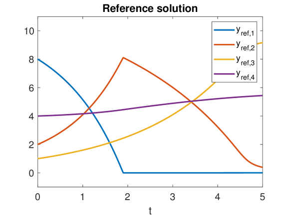
Figure 16: Reference solution of the NPZD problem (32) plotted over the time interval $[0,5]$ in hours.

It was demonstrated in [22] that the occurrence of negative approximations leads to the divergence of the method, and hence, severe time step restrictions to schemes not preserving the positivity unconditionally are necessary. For the numerical experiments we use an initial time step size of $\Delta t_{0}=1$.

Appendix B Validation Problems

Here we introduce several validation problems. In particular, we consider the Prothero and Robinson problem with other parameters and the Brusselator problem.

B.1 Prothero & Robinson Problem

As we have constructed infinitely many problems (27), it is an obvious decision to also take some of the test cases as a validation problem. In particular, we use $\xi\in\{0.1,0.3,0.5\}$.

B.2 Brusselator Problem

As a non-stiff validation problem we consider the Brusselator problem [62, 2] which reads

$$y_{1}^{\prime} =-k_{1}y_{1},$$ (33)

$$y_{2}^{\prime} =-k_{2}y_{2}y_{5},$$

$$y_{3}^{\prime} =k_{2}y_{2}y_{5},$$

$$y_{4}^{\prime} =k_{4}y_{5},$$

$$y_{5}^{\prime} =k_{1}y_{1}-k_{2}y_{2}y_{5}+k_{3}y_{5}^{2}y_{6}-k_{4}y_{5},$$

$$y_{6}^{\prime} =k_{2}y_{2}y_{5}-k_{3}y_{5}^{2}y_{6},$$

where we set $k_{i}>0$. In form of PDS the Brusselator problem is determined by

$$p_{32}(\mathbf{y}) =k_{2}y_{2}y_{5}, p_{45}(\mathbf{y}) =k_{4}y_{5}, p_{51}(\mathbf{y}) =k_{1}y_{1},$$

$$p_{56}(\mathbf{y}) =k_{3}y_{5}^{2}y_{6}, p_{65}(\mathbf{y}) =k_{2}y_{2}y_{5}$$

and $d_{ij}=p_{ji}$. We set $k_{i}=1$ and use the initial condition $\mathbf{y}(0)=(10,10,0,0,0.1,0.1)^{T}$. The time interval of interest is $[0,10]$, and the reference solution can be seen in Figure 17. The numerical method start with a time step size of $\Delta t_{0}=0.1$.

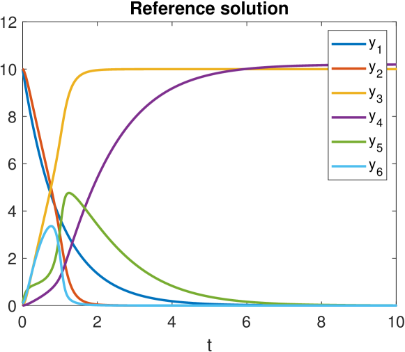
Figure 17: Reference solution of the Brusselator problem (33) plotted over the time interval $[0,10]$.

References

- \bibcommenthead
- Butcher [2016] Butcher, J.C.: Numerical Methods for Ordinary Differential Equations, 3rd edn., p. 513. John Wiley & Sons, Ltd., Chichester (2016). With a foreword by J. M. Sanz-Serna. https://doi.org/10.1002/9781119121534
- Hairer et al. [1993] Hairer, E., Nørsett, S.P., Wanner, G.: Solving Ordinary Differential Equations I. Nonstiff Problems, 2nd edn. Springer Series in Computational Mathematics, vol. 8, p. 528. Springer, Berlin (1993). https://doi.org/%****␣Manuscript.bbl␣Line␣75␣****10.1007/978-3-540-78862-1
- Hairer and Wanner [2010] Hairer, E., Wanner, G.: Solving Ordinary Differential Equations II. Stiff and Differential-algebraic Problems. Springer Series in Computational Mathematics, vol. 14, p. 614. Springer, Berlin (2010). https://doi.org/10.1007/978-3-642-05221-7 . Second revised edition, paperback
- Gustafsson et al. [1988] Gustafsson, K., Lundh, M., Söderlind, G.: A PI stepsize control for the numerical solution of ordinary differential equations. BIT Numerical Mathematics 28(2), 270–287 (1988) https://doi.org/10.1007/BF01934091
- Gustafsson [1991] Gustafsson, K.: Control theoretic techniques for stepsize selection in explicit Runge-Kutta methods. ACM Transactions on Mathematical Software (TOMS) 17(4), 533–554 (1991) https://doi.org/10.1145/210232.210242
- Söderlind [2006] Söderlind, G.: Time-step selection algorithms: Adaptivity, control, and signal processing. Applied Numerical Mathematics 56(3-4), 488–502 (2006) https://doi.org/10.1016/j.apnum.2005.04.026
- Söderlind and Wang [2006] Söderlind, G., Wang, L.: Adaptive time-stepping and computational stability. Journal of Computational and Applied Mathematics 185(2), 225–243 (2006) https://doi.org/10.1016/j.cam.2005.03.008
- Söderlind [2002] Söderlind, G.: Automatic control and adaptive time-stepping. Numer. Algorithms 31(1-4), 281–310 (2002) https://doi.org/10.1023/A:1021160023092 . Numerical methods for ordinary differential equations (Auckland, 2001)
- Söderlind [2003] Söderlind, G.: Digital filters in adaptive time-stepping. ACM Transactions on Mathematical Software (TOMS) 29(1), 1–26 (2003) https://doi.org/10.1145/641876.641877
- Zonneveld [1964] Zonneveld, J.A.: Automatic Numerical Integration. Mathematical Centre Tracts, vol. 8, p. 110. Mathematisch Centrum, Amsterdam (1964). https://ir.cwi.nl/pub/13099
- Gustafsson [1994] Gustafsson, K.: Control-theoretic techniques for stepsize selection in implicit Runge-Kutta methods. ACM Trans. Math. Software 20(4), 496–517 (1994) https://doi.org/10.1145/198429.198437
- Arévalo and Söderlind [2017] Arévalo, C., Söderlind, G.: Grid-independent construction of multistep methods. J. Comput. Math. 35(5), 672–692 (2017) https://doi.org/10.4208/jcm.1611-m2015-0404
- Ranocha et al. [2022] Ranocha, H., Dalcin, L., Parsani, M., Ketcheson, D.I.: Optimized Runge-Kutta methods with automatic step size control for compressible computational fluid dynamics. Commun. Appl. Math. Comput. 4(4), 1191–1228 (2022) https://doi.org/10.1007/s42967-021-00159-w
- Bull [2011] Bull, A.D.: Convergence rates of efficient global optimization algorithms. J. Mach. Learn. Res. 12, 2879–2904 (2011)
- Gelbart et al. [2014] Gelbart, M.A., Snoek, J., Adams, R.P.: Bayesian optimization with unknown constraints. In: Proceedings of the Thirtieth Conference on Uncertainty in Artificial Intelligence. UAI’14, pp. 250–259. AUAI Press, Arlington, Virginia, USA (2014)
- Snoek et al. [2012] Snoek, J., Larochelle, H., Adams, R.P.: Practical bayesian optimization of machine learning algorithms. In: Pereira, F., Burges, C.J., Bottou, L., Weinberger, K.Q. (eds.) Advances in Neural Information Processing Systems, vol. 25. Curran Associates, Inc. (2012). https://proceedings.neurips.cc/paper_files/paper/2012/file/05311655a15b75fab86956663e1819cd-Paper.pdf
- Jackiewicz [2009] Jackiewicz, Z.a.: General Linear Methods for Ordinary Differential Equations, p. 482. John Wiley & Sons, Inc., Hoboken, New Jersey (2009). https://doi.org/10.1002/9780470522165
- Bolley and Crouzeix [1978] Bolley, C., Crouzeix, M.: Conservation de la positivité lors de la discrétisation des problèmes d’évolution paraboliques. RAIRO Anal. Numér. 12(3), 237–245 (1978) https://doi.org/10.1051/m2an/1978120302371
- Sandu [2002] Sandu, A.: Time-stepping methods that favor positivity for atmospheric chemistry modeling. In: Atmospheric Modeling (Minneapolis, MN, 2000). IMA Vol. Math. Appl., vol. 130, pp. 21–37. Springer, New York (2002). https://doi.org/10.1007/978-1-4757-3474-4_2
- Shampine et al. [2005] Shampine, L.F., Thompson, S., Kierzenka, J.A., Byrne, G.D.: Non-negative solutions of ODEs. Appl. Math. Comput. 170(1), 556–569 (2005) https://doi.org/%****␣Manuscript.bbl␣Line␣350␣****10.1016/j.amc.2004.12.011
- Kopecz and Meister [2019] Kopecz, S., Meister, A.: A comparison of numerical methods for conservative and positive advection-diffusion-production-destruction systems. PAMM 19(1), 201900209 (2019) https://doi.org/10.1002/pamm.201900209
- Burchard et al. [2005] Burchard, H., Deleersnijder, E., Meister, A.: Application of modified Patankar schemes to stiff biogeochemical models for the water column. Ocean Dynamics 55(3), 326–337 (2005) https://doi.org/10.1007/s10236-005-0001-x
- Huang and Shu [2019] Huang, J., Shu, C.-W.: Positivity-preserving time discretizations for production-destruction equations with applications to non-equilibrium flows. J. Sci. Comput. 78(3), 1811–1839 (2019) https://doi.org/10.1007/s10915-018-0852-1
- Sandu [2001] Sandu, A.: Positive numerical integration methods for chemical kinetic systems. J. Comput. Phys. 170(2), 589–602 (2001) https://doi.org/10.1006/jcph.2001.6750
- Nüsslein et al. [2021] Nüsslein, S., Ranocha, H., Ketcheson, D.I.: Positivity-preserving adaptive Runge-Kutta methods. Commun. Appl. Math. Comput. Sci. 16(2), 155–179 (2021) https://doi.org/%****␣Manuscript.bbl␣Line␣425␣****10.2140/camcos.2021.16.155
- Patankar [1980] Patankar, S.V.: Numerical Heat Transfer and Fluid Flow. Series in computational methods in mechanics and thermal sciences. Hemisphere Pub. Corp. New York, Washington (1980). http://opac.inria.fr/record=b1085925
- Shampine [1986] Shampine, L.F.: Conservation laws and the numerical solution of ODEs. Comput. Math. Appl. Part B 12(5-6), 1287–1296 (1986) https://doi.org/10.1016/0898-1221(86)90253-1
- Burchard et al. [2003] Burchard, H., Deleersnijder, E., Meister, A.: A high-order conservative Patankar-type discretisation for stiff systems of production-destruction equations. Appl. Numer. Math. 47(1), 1–30 (2003) https://doi.org/10.1016/S0168-9274(03)00101-6
- Kopecz and Meister [2018a] Kopecz, S., Meister, A.: On order conditions for modified Patankar-Runge-Kutta schemes. Appl. Numer. Math. 123, 159–179 (2018) https://doi.org/10.1016/j.apnum.2017.09.004
- Kopecz and Meister [2018b] Kopecz, S., Meister, A.: Unconditionally positive and conservative third order modified Patankar-Runge-Kutta discretizations of production-destruction systems. BIT 58(3), 691–728 (2018) https://doi.org/10.1007/s10543-018-0705-1
- Araújo et al. [1997] Araújo, A.L., Murua, A., Sanz-Serna, J.M.: Symplectic methods based on decompositions. SIAM J. Numer. Anal. 34(5), 1926–1947 (1997) https://doi.org/10.1137/S0036142995292128
- Izgin et al. [2023] Izgin, T., Ketcheson, D.I., Meister, A.: Order conditions for Runge–Kutta-like methods with solution-dependent coefficients. https://arxiv.org/abs/2305.14297 (2023) https://doi.org/10.48550/arXiv.2305.14297
- Öffner and Torlo [2020] Öffner, P., Torlo, D.: Arbitrary high-order, conservative and positivity preserving Patankar-type deferred correction schemes. Appl. Numer. Math. 153, 15–34 (2020) https://doi.org/10.1016/j.apnum.2020.01.025
- Ciallella et al. [2022] Ciallella, M., Micalizzi, L., Öffner, P., Torlo, D.: An arbitrary high order and positivity preserving method for the shallow water equations. Comput. & Fluids 247, 105630–21 (2022) https://doi.org/10.1016/j.compfluid.2022.105630
- Ávila et al. [2020] Ávila, A.I., Kopecz, S., Meister, A.: A comprehensive theory on generalized BBKS schemes. Appl. Numer. Math. 157, 19–37 (2020) https://doi.org/10.1016/j.apnum.2020.05.027
- Martiradonna et al. [2020] Martiradonna, A., Colonna, G., Diele, F.: GeCo: Geometric Conservative nonstandard schemes for biochemical systems. Appl. Numer. Math. 155, 38–57 (2020) https://doi.org/10.1016/j.apnum.2019.12.004
- Huang et al. [2019] Huang, J., Zhao, W., Shu, C.-W.: A third-order unconditionally positivity-preserving scheme for production-destruction equations with applications to non-equilibrium flows. J. Sci. Comput. 79(2), 1015–1056 (2019) https://doi.org/10.1007/s10915-018-0881-9
- Izgin et al. [2022a] Izgin, T., Kopecz, S., Meister, A.: On Lyapunov stability of positive and conservative time integrators and application to second order modified Patankar–Runge–Kutta schemes. ESAIM Math. Model. Numer. Anal. 56(3), 1053–1080 (2022) https://doi.org/10.1051/m2an/2022031
- Izgin et al. [2022b] Izgin, T., Kopecz, S., Meister, A.: On the stability of unconditionally positive and linear invariants preserving time integration schemes. SIAM J. Numer. Anal. 60(6), 3029–3051 (2022) https://doi.org/10.1137/22M1480318
- Izgin et al. [2023] Izgin, T., Kopecz, S., Meister, A.: A stability analysis of modified Patankar–Runge–Kutta methods for a nonlinear production–destruction system. PAMM 22(1), 202200083 (2023) https://doi.org/10.1002/pamm.202200083
- Izgin and Öffner [2023] Izgin, T., Öffner, P.: A study of the local dynamics of modified Patankar DeC and higher order modified Patankar–RK methods. ESAIM Math. Model. Numer. Anal. 57(4), 2319–2348 (2023) https://doi.org/10.1051/m2an/2023053
- Izgin et al. [2023] Izgin, T., Kopecz, S., Martiradonna, A., Meister, A.: On the dynamics of first and second order GeCo and gBBKS schemes. Applied Numerical Mathematics 193, 43–66 (2023) https://doi.org/10.1016/j.apnum.2023.07.014
- Torlo et al. [2022] Torlo, D., Öffner, P., Ranocha, H.: Issues with positivity-preserving Patankar-type schemes. Appl. Numer. Math. 182, 117–147 (2022) https://doi.org/10.1016/j.apnum.2022.07.014
- Izgin et al. [2022] Izgin, T., Öffner, P., Torlo, D.: A necessary condition for non oscillatory and positivity preserving time-integration schemes. https://arxiv.org/abs/2211.08905 (2022) https://doi.org/10.48550/ARXIV.2211.08905
- Kopecz et al. [2021] Kopecz, S., Meister, A., Podhaisky, H.: On adaptive patankar runge–kutta methods. PAMM 21(1), 202100235 (2021) https://doi.org/10.1002/pamm.202100235
- Formaggia and Scotti [2011] Formaggia, L., Scotti, A.: Positivity and conservation properties of some integration schemes for mass action kinetics. SIAM J. Numer. Anal. 49(3), 1267–1288 (2011) https://doi.org/10.1137/100789592
- Ávila et al. [2021] Ávila, A.I., González, G.J., Kopecz, S., Meister, A.: Extension of modified Patankar-Runge-Kutta schemes to nonautonomous production-destruction systems based on Oliver’s approach. J. Comput. Appl. Math. 389, 113350–13 (2021) https://doi.org/10.1016/j.cam.2020.113350
- Ralston and Rabinowitz [2001] Ralston, A., Rabinowitz, P.: A First Course in Numerical Analysis, 2nd edn., pp. 556–50. Dover Publications, Inc., Mineola, New York (2001). https://www.biblio.com/9780070511583?placement=basic-info
- Carr [1981] Carr, J.: Applications of Centre Manifold Theory. Applied Mathematical Sciences, vol. 35, p. 142. Springer, New York (1981). https://doi.org/10.1007/978-1-4612-5929-9
- Stuart and Humphries [1998] Stuart, A., Humphries, A.R.: Dynamical Systems and Numerical Analysis vol. 2. Cambridge University Press, Cambridge (1998)
- Watts [1984] Watts, H.A.: Step size control in ode solvers (1984)
- Hall and Higham [1988] Hall, G., Higham, D.J.: Analysis of stepsize selection schemes for Runge-Kutta codes. IMA Journal of Numerical Analysis 8(3), 305–310 (1988) https://doi.org/10.1093/imanum/8.3.305
- Higham and Hall [1990] Higham, D.J., Hall, G.: Embedded Runge-Kutta formulae with stable equilibrium states. Journal of Computational and Applied Mathematics 29(1), 25–33 (1990) https://doi.org/10.1016/0377-0427(90)90192-3
- Ranocha and Giesselmann [2023] Ranocha, H., Giesselmann, J.: Stability of Step Size Control Based on a Posteriori Error Estimates. https://doi.org/10.48550/arXiv.2307.12677
- MathWorks [2023] MathWorks: MATLAB. (2023). https://www.mathworks.com/products/new_products/latest_features.html
- Shampine and Reichelt [1997] Shampine, L.F., Reichelt, M.W.: The MATLAB ODE suite. SIAM Journal on Scientific Computing 18(1), 1–22 (1997) https://doi.org/10.1137/S1064827594276424
- [57] Bleecke, S., Ranocha, H.: Step Size Control for Explicit Relaxation Runge-Kutta Methods Preserving Invariants. https://doi.org/10.48550/arXiv.2311.14050
- Prothero and Robinson [1974] Prothero, A., Robinson, A.: On the stability and accuracy of one-step methods for solving stiff systems of ordinary differential equations. Math. Comp. 28, 145–162 (1974) https://doi.org/10.2307/2005822
- Benvenuti and Farina [2004] Benvenuti, L., Farina, L.: Eigenvalue regions for positive systems. Systems & Control Letters 51(3-4), 325–330 (2004) https://doi.org/10.1016/j.sysconle.2003.09.009
- Schäfer [1975] Schäfer, E.: A new approach to explain the “high irradiance responses” of photomorphogenesis on the basis of phytochrome. Journal of Mathematical Biology 2, 41–56 (1975) https://doi.org/10.1007/BF00276015
- Mazzia et al. [2003] Mazzia, F., Iavernaro, F., Magherini, C.: Test set for initial value problem solvers. Department of Mathematics, University of Bari (2003)
- Lefever and Nicolis [1971] Lefever, R., Nicolis, G.: Chemical instabilities and sustained oscillations. Journal of Theoretical Biology 30(2), 267–284 (1971) https://doi.org/10.1016/0022-5193(71)90054-3