Study of isospin diffusion from ^40,48Ca$+^{40,48}$Ca experimental data at Fermi energies: direct comparisons with transport model calculations

Abstract

This article presents an investigation of isospin equilibration in cross-bombarding ^40,48Ca$+^{40,48}$Ca reactions at $35$ MeV/nucleon, by comparing experimental data with filtered transport model calculations. Isospin diffusion is studied using the evolution of the isospin transport ratio with centrality. The asymmetry parameter $\delta=(N-Z)/A$ of the quasiprojectile (QP) residue is used as isospin-sensitive observable, while a recent method for impact parameter reconstruction is used for centrality sorting. A benchmark of global observables is proposed to assess the relevance of the antisymmetrized molecular dynamics (AMD) model, coupled to GEMINI++, in the study of dissipative collisions. Our results demonstrate the importance of considering cluster formation to reproduce observables used for isospin transport and centrality studies. Within the AMD model, we prove the applicability of the impact parameter reconstruction method, enabling a direct comparison to the experimental data for the investigation of isospin diffusion. For both, we evidence a tendency to isospin equilibration with an impact parameter decreasing from $9$ to $3$ fm, while the full equilibration is not reached. A weak sensitivity to the stiffness of the equation of state employed in the model is also observed, with a better reproduction of the experimental trend for the neutron-rich reactions.

I Introduction

The nuclear equation of state (EoS) is a major issue in modern astrophysics and nuclear physics, as it is a central ingredient in the modeling of core-collapse supernovae, neutron stars and compact binary stars mergers Lattimer and Prakash (2016), but also in heavy ion collisions (HIC) dynamics and nuclear structure Toro et al. (2010). Many efforts are nowadays dedicated to the study of the density dependence of the nuclear matter symmetry energy Tsang et al. (2012); Lattimer and Lim (2013); Huth et al. (2022); Lynch and Tsang (2022). This term represents the energy cost of converting all protons in symmetric matter into neutrons (at fixed temperature and density), and it is usually defined as the second derivative of the energy per nucleon in nuclear matter with respect to the neutron-to-proton asymmetry (isospin). Better knowledge of the symmetry energy is necessary in the context of astrophysical simulations which aim to describe neutron-rich systems over a wide range of densities. At supra-saturation densities, constraints can be extracted by relativistic HIC Russotto et al. (2011) and multi-messenger measurements Abbott et al. (2017), whose interest has been renewed by the recent breakthrough in gravitational waves measurements. At sub-saturation, HIC offer a unique opportunity to study the modification of the chemical composition induced by the formation and dissolution of clusters in dilute nuclear matter Typel (2013). The study of these reactions allows to probe the thermodynamical properties of the expanding nuclear system, thus the effect of cluster formation on the symmetry energy. Various HIC observables have been used to study the symmetry energy density dependence of neutron-rich matter. Experimental probes such as nuclear masses Brown (2013), isobaric analog states Danielewicz and Lee (2014), collective flows Russotto et al. (2016), pion yield ratios Estee et al. (2021) and isospin transport Tsang et al. (2009a) have been used to constrain the symmetry energy functional. More recently, it has been shown that such measurements are not only consistent with astrophysical observations but they also provide important constraints on the nuclear EoS at supra-saturation densities Huth et al. (2022); Lynch and Tsang (2022). It was furthermore pointed out that improvements in the interpretation of experimental observables are needed if one wants to refine our knowledge of the EoS. In this context, isospin transport is particularly interesting as it led to one of the first experimental constraints on the symmetry energy Tsang et al. (2009b). This process, expected to occur in binary dissipative reactions, corresponds to a stochastic and differential exchange of nucleons between projectile and target. In particular, in collisions with different projectile and target $N/Z$ asymmetries, a balancing in the neutron-richness of different isospin regions is expected to take place, leading to a rearrangement of the neutron-to-proton ratio of the colliding nuclei, called isospin diffusion. The degree of isospin equilibration, directly related to the magnitude of the symmetry energy (at a given local density), can be experimentally estimated from the isospin transport ratio Rami et al. (2000), widely used over the years Camaiani et al. (2020, 2021); Piantelli et al. (2021); Ciampi et al. (2022); Fable et al. (2023).

Constraints on the EoS are obtained by comparing nuclear experimental data to transport model calculation, where it is possible to test the interplay between the mean-field effects and nucleon-nucleon collisions. In addition to the inherent difficulty of implementing various algorithms for solving the transport equations, uncertainties also arise from the comparison protocols between the experimental data and the transport models. Indeed, as most of the relevant observables are not directly measurable experimentally, surrogate variables are usually used, complicating the interpretations. Suitable comparisons should therefore focus on an identical set of observables, with calculations ideally run over the same domain of impact parameter probed by the experiment and taking into account the intrinsic limits of the experimental setup. To this aim, this work presents an investigation of isospin diffusion in ^40,48Ca$+^{40,48}$Ca reactions at $35$ MeV/nucleon, from both experimental and transport model simulation data. The experimental setup is described in Sec.II. The model framework is discussed in Sec.III along with global comparisons with the experimental data. The impact parameter estimation method is presented in Sec.IV, while the results on isospin diffusion are presented in Sec.V. A summary and conclusions are finally drawn in Sec.VI.

II Experimental setup and event selection

II.1 Experimental setup

The experiment was performed at the GANIL facility, where beams of ^40,48Ca at 35 MeV/nucleon impinged on self-supporting $1.0$ mg/cm^{2 40}Ca or $1.5$ mg/cm^{2 48}Ca targets placed inside the INDRA vacuum chamber, for a typical beam intensity around $5.10^{7}$ pps. The detection apparatus consisted of the coupling of the $4\pi$ charged particle array INDRA and the VAMOS high-acceptance spectrometer. INDRA is composed of detection telescopes arranged in rings and centered around the beam axis. A detailed description of the INDRA detector and its electronics can be found in Pouthas et al. (1995, 1996). For this experiment, INDRA covered polar angles from $7^{\circ}$ to $176^{\circ}$, as rings 1 to 3 were removed to allow the mechanical coupling with VAMOS in the forward direction. Rings 4 to 9 ($7^{\circ}-45^{\circ}$) consisted each of 24 three-layer detection telescopes: a gas-ionization chamber operated with C₃F₈ gas at low pressure, a 300 or 150 $\mu$m silicon wafer, and a CsI(Tl) scintillator (14 to 10 cm thick) read by a photomultiplier tube. Rings 10 to 17 ($45^{\circ}-176^{\circ}$) included 24, 16, or 8 two-layer telescopes: a gas-ionization chamber and a CsI(Tl) scintillator of 8, 6, or 5 cm thickness. Fragment identification thresholds were about $0.5$ and $1.5$ MeV/nucleon for the lightest ($Z\lesssim 10$) and the heaviest fragments, respectively. INDRA allowed charge and isotope identification up to Be-B and charge identification for heavier fragments.

VAMOS is composed of two large magnetic quadrupoles focusing the incoming ions in the vertical and horizontal planes, followed by a large magnetic dipole Pullanhiotan et al. (2008); Lemasson and Rejmund (2023). In the used configuration, the spectrometer was rotated at $4.5^{\circ}$ with respect to the beam axis, to cover the forward polar angles from $2.56^{\circ}$ to $6.50^{\circ}$, favoring the detection of a fragment emitted slightly above the grazing angles of the studied reactions. The momentum acceptance was about $\pm 5\%$ and the focal plane was located $9$ m downstream the target, giving a large enough time of flight (ToF) base to obtain a mass resolution of about $\Delta A/A\approx 1/165$ for the isotopes produced in the collisions. VAMOS detection setup included two position-sensitive drift chambers used to determine the trajectories of the reaction products at the focal plane, followed by a seven-module ionization chamber, a 500 $\mu$m thick Si wall (18 independent modules), and a $1$ cm thick CsI(Tl) wall (80 independent modules), allowing the measurements of the ToF, energy loss ($\Delta E$), and energy ($E$) parameters. Around 12 magnetic rigidity settings, from $0.661$ to $2.220$ Tm, were used for each system to cover the full velocity range of the fragments. At least one hit on the VAMOS silicon wall was required for each event to be acquired.

An overview of the acquired data has been presented in Fable et al. (2022), with a detailed description of the identification, reconstruction and event normalization procedures. In a second paper, a study dedicated to isospin diffusion and migration was presented, demonstrating the potential of the INDRA-VAMOS coupling to provide further experimental constraints on the nuclear symmetry energy Fable et al. (2023).

II.2 Data selection

The following preliminary selections have been applied for the present analysis :

i) Only multiplicity “$1"$ events in the VAMOS Si wall were considered. This offline selection was applied to make sure that the positions measured in the drift chambers are correct and to remove events with ambiguous trajectory reconstruction.

ii) Elastic-like events, defined as events with no hit in INDRA and a fragment identical to the projectile in VAMOS, were also removed offline.

iii) The most incomplete events were discarded by requesting a measured total charge $Z_{tot}\geq 10$ and a total parallel momentum (along the beam axis) $p_{z}^{tot}\geq 0.5\cdot p_{beam}$, where $p_{beam}$ is the beam initial momentum.

iv) Events with a potential QP residue measured in INDRA were discarded by requesting that $Z_{PLF}>Z_{I}^{max,fwd}$, where $Z_{PLF}$ and $Z_{I}^{max,fwd}$ are respectively the charge of the fragment detected in VAMOS and of the heaviest fragment forward-emitted in the reaction center of mass (c.m.) identified in charge with INDRA. Since we focus on the study of isospin-sensitive observables from the QP remnant, such events are indeed not relevant due to the limited mass identification ($Z\lesssim 5$) with INDRA.

In summary, the applied data selections criteria represent a subset of about $90\%$ and $87\%$ of the total statistics of the experimental data for ⁴⁰Ca and ⁴⁸Ca projectile reactions, respectively.

III Simulation codes and global comparisons

III.1 Antisymmetrized molecular dynamics

The present analysis relies on the comparison of experimental data with the output of the antisymmetrized molecular dynamics (AMD) model Ono et al. (1992). AMD is a microscopic transport model widely used to describe various features of ground state nuclei Kanada-En’yo et al. (2003) and out of equilibrium many-body dynamics Ono (2013), recently reviewed in Wolter et al. (2022).

A general issue encountered when comparing transport model simulations with experimental HIC data at Fermi energies is the underestimation of light cluster yields. For example, in a recent study Frosin et al. investigated the role of clustering at Fermi energies by comparing ³²S$+^{12}$C and ²⁰Ne$+^{12}$C reactions at 25 and 50 MeV/nucleon measured with four FAZIA blocks with the output of the AMD model Frosin et al. (2023). It was shown that accounting for cluster formation helps to better reproduce experimental multiplicities of both light-charged particles (LCP, $Z\leq 2$) and intermediate mass fragments (IMF, $3\leq Z\leq 8$) but also their kinetic energy distributions. Furthermore, to our knowledge, in the literature very few works adressed the specific issue of clustering in semi-peripheral to peripheral collisions, where binary dissipative collisions exhaust a large part of the total reaction cross section Piantelli et al. (2017).

In this perspective, we present in this section a comparison of the INDRA-VAMOS data with a basic version of AMD, namely AMD-NC, and a more recent version with cluster correlations, namely AMD-CC. More precisely, in AMD-CC cluster correlations are explicitly taken into account by allowing each of the scatterd nucleons to form light clusters ($A\leq 4$) and also heavier nuclei (up to $A\lesssim 10$) from the introduction of intercluster correlations as a stochastic process of intercluster binding, as described in Ono (2019).

Concerning AMD-NC, the same version as the one detailed in Ono (1999) was employed, proven to be suitable for the study of Ca+Ca collisions at 35 MeV/nucleon Wada et al. (1998); Ono et al. (2004). This version was used in our previous work on isoscaling Fable et al. (2022) and isospin transport Fable et al. (2023). Collisions were followed up to $t_{lim}=300$ fm/c, for a total of approximately $100000$ primary events per system. Clusters were defined at $t_{lim}$ according to a proximity criterion of the Gaussian centroids in spatial coordinates, two-nucleon pair separated by less than 5 fm contributing to the formation of a cluster. In this version the mean-field description is based on the momentum-dependent Gogny force, consistent with the incompressibility modulus of symmetric matter $K_{sat}=228$ MeV and $\rho_{0}=0.16$ fm^-3. Based on such effective interaction, two parametrizations of the density-dependence of the nuclear symmetry energy were exploited, namely the Gogny (soft dependence) and Gogny-AS (stiff dependence) forces Dechargé and Gogny (1980).

Concerning AMD-CC, we have employed the same simulated data as those published in Camaiani et al. (2020). Collisions were followed up to $t_{lim}=500$ fm/c, for a total of about $40000$ primary events per system. In this version, the mean-field description is based on the momentum-dependent SLy4 effective Skyrme interaction Chabanat et al. (1997), with $K_{sat}=230$ MeV and $\rho_{0}=0.16$ fm^-3. Two parametrizations of the symmetry energy were tested: a soft symmetry energy dependence with $E_{sym}=32$ MeV and $L=46$ MeV, as zero and first order terms, respectively, and a stiff one with $L=108$ MeV. Finally, a reduction factor of $\gamma=0.85$ was employed for the in-medium correction of nucleon-nucleon cross-section, following the prescription proposed in Lopez et al. (2014).

For both models, the input impact parameter followed a triangular distribution from $0$ to a value $b_{max}$, that is slightly above the geometrical grazing impact parameter $b_{gr}$ (about $9.7$ fm for ⁴⁰Ca$+^{40}$Ca and $10.4$ fm for ⁴⁸Ca$+^{48}$Ca). The statistical decay code GEMINI++ was employed Charity (2010) to de-excite the hot nuclei produced at $t_{lim}$ (afterburner step), using the default parameters of the code, for a total of 50 and 100 secondary events per primary event for AMD-NC and AMD-CC respectively. The number of decays per primary event was chosen to limit their effect on the uncertainties associated to the imbalance ratio.

We note an important discrepancy between the two versions of AMD, due to the difference in stopping time $t_{lim}$. Indeed, in our former work with AMD-NC we have employed a standard $t_{lim}$ value widely used in the literature with this version of the code Ono et al. (2004). In comparison, in the case of AMD-CC the authors of ref. Camaiani et al. (2021) ensured that the primary fragments have reached thermodynamical equilibrium (while Coulomb repulsion is negligible) at $t_{lim}$, for the systems under study Piantelli et al. (2019). Given the previous comment, some caveats are to be considered when comparing the primary events of the two model versions.

III.2 Filter and event selection

For both aforementioned versions of the AMD model, simulated events were filtered with the same software replica of the experimental setup, to allow comparison between the predictions and the experimental data.

Event detection was simulated within the KaliVeda framework Frankland et al. (2023). Concerning VAMOS, the experimental polar and azimuthal angular distribution in the laboratory frame were used to apply cuts on the simulated events, while the energy and identification thresholds of the Si and CsI detectors were considered. Concerning INDRA, KaliVeda allows a complete description of the detector configuration for the experiment, including geometrical coverage, dead-zones, detector resolutions and identification thresholds. It must be noted that the majority of the simulated events are discarded due to the spectrometer angular acceptance and trigger condition, for a total of about $\approx 75\%$ of the whole statistics.

In addition to the numerical filtering, the same offline selections as the experiment, described in Sec.II.1, were applied to the filtered events. In summary, once the preliminary selections are applied, the filtered simulated events represent a subset of about of $22\%$ and $18\%$ of the total statistics for the AMD-CC and AMD-NC models, respectively.

III.3 General features

In this section we present a comparison of several relevant global observables between the two versions of the AMD model, to better apprehend the results on isospin diffusion presented in the next section. For the sake of clarity and as we focus on the general features, only the results obtained from a soft symmetry energy are presented at this point of the analysis.

III.3.1 Topology of the reaction products

Figure 1 depicts the correlations between the charge and the parallel velocity (laboratory frame) for all particles identified in charge in the ⁴⁸Ca$+^{48}$Ca reactions, for the experiment (a) and the AMD-CC model without (b) and with (c) filter and event selection criteria.

Similarly to our previous work with the AMD-NC version Fable et al. (2022), the unfiltered model exhibits two main components on both sides of the c.m. velocity (black dashed line), with a third region of LCP and IMF spreading over the whole velocity domain. By comparing the unfiltered and filtered simulations, we mainly observe the effect of VAMOS angular acceptance, which drastically reduces the measured yields while the right-most component becomes concentrated in a region of charge and velocity close to the projectile one. Such topology is representative of dissipative binary collisions, where the fragments detected in VAMOS are mostly the products of the quasiprojectile decay (namely the projectile-like fragment, PLF) resulting from peripheral to semi-peripheral collisions, while the products of the quasitarget (target-like fragment, TLF) decay are occasionally identified in INDRA at backward angles (left-most component). Finally, by comparing the experimental data and the filtered model, a satisfactory agreement is observed. It must be noted that similar topologies are observed independently of the version of the AMD model and for all the systems, with a similar effect of the numerical filter and data selection Fable et al. (2022).

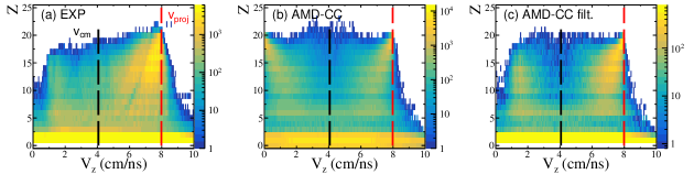
Figure 1: Atomic number $Z$ as a function of the parallel velocity $V_{z}$ (in the laboratory frame) for the ⁴⁸Ca$+^{48}$Ca system. Experimental data (a). Secondary fragments from AMD-CC (after GEMINI++ de-excitation) without (b) or with (c) the experimental filter. The black and red dashed vertical lines indicate the reaction c.m. and the projectile velocities, respectively.

We present in Fig. 2 the effect of the filter and event selection criteria on the reduced impact parameter distributions for the ⁴⁸Ca$+^{48}$Ca system. The input triangular distributions, represented as solid lines, present a small difference between the models as AMD-CC was ran up to slightly larger $b/b_{max}$ values than AMD-NC. Interestingly, we observe a strong difference between the two versions of the code once the filter and data selection are applied, AMD-NC (open circles) leading to the detection of more peripheral events compared to AMD-CC (full circles), even if the latter was run up to higher impact parameter values. Such remarkable difference is not trivial as it comes from the combined effect of the model dynamics, the detectors acceptance and the applied offline selections. In a sense, this plot highlights the inherent difficulty of comparing models with experimental data as the subset of simulated data can vary from a model to another, before and even more after the numerical filtering and data selections are applied.

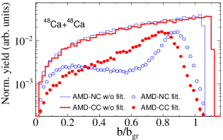
Figure 2: Reduced impact parameter distributions from filterd AMD-NC (open circles) and AMD-CC (full circles) models with data selection. Solid lines correspond to the input triangular distributions. The plots are normalized to the integral of their respective input distributions.

Indeed, it is for example expected that the AMD-NC version leads, in average, to more LCP emissions compared to AMD-CC, therefore to a different pattern of multiplicities and kinetic energy spectra. In fact, a more detailed study of the primary fragments from AMD-NC (not presented here) leads to the conclusion that this version of the code tends to overproduce inelastic collisions in the $b/b_{max}=0.8-1$ region as compared to AMD-CC, while these fragments have still enough excitation energy to emit LCP in the afterburner phase.

III.3.2 Study of the QP residue

We present in this section a comparison of the global observables related to the fragment detected in VAMOS, expected to be the QP remnant (PLF). According to the simulations, more than $95\%$ of the nuclei detected in VAMOS (after data selection criteria) correspond to the remnant of the QP, the latter defined as the biggest primary fragment forward emitted in the c.m. reference frame.

The parallel velocity (laboratory frame) and charge distributions of the filtered PLF are given in Figs. 3(a-d) and (e-h) respectively, for the four reactions under study. The main plots present the distributions obtained from the experiment (full circles) and filtered models (continuous lines) when the selection criteria are applied. Concerning the velocity distributions (top panels), we observe decreasing values of the yields with decreasing velocity of the PLF, reflecting the impact parameter distribution. As expected from Fig. 2, the differences between the two versions of AMD are more pronounced for the most peripheral collisions ($b/b_{gr}\simeq 0.8$, $V_{z}\simeq 8$ cm/ns) as AMD-NC tends to overproduce inelastic-like events compared to AMD-CC. It is interesting to note that the opposite effect is observed for the unfiltered models represented in the inner plots, showing that the experimental selection criteria (and indirectly the consideration of cluster formation) may have a strong impact on the filtered distributions. An overall better agreement with experimental data is obtained with AMD-CC, while it tends to produce slighlty slower QP compared to the experiment and AMD-NC. Similar results were obtained from various systems simulated with AMD-CC followed by GEMINI++ as afterburner Piantelli et al. (2021); Camaiani et al. (2021); Ciampi et al. (2022), and it was concluded that the model is more dissipative than the experimental case, although the effect of the filter, event selection (event multiplicity) and clustering process were not detailed. Concerning the atomic number distributions (bottom panels), similar conclusions can be drawn: AMD-CC reproduces remarkably well the charge distributions for all the systems, even for the neutron-rich ⁴⁸Ca$+^{48}$Ca, while AMD-NC predicts more heavy products than experimentally observed. The same conclusion can also be drawn from the mass distributions of the PLF (not shown here). Finally, it is interesting to note that the observed experimental odd-even staggering Piantelli et al. (2013), stronger for neutron-deficient systems, is partially reproduced by both filtered simulations, as a consequence of the sequential decays (GEMINI++).

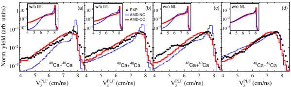
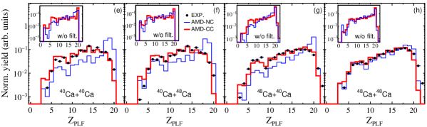
Figure 3: Parallel velocity (a-d) and charge (e-h) distributions of the PLF from the experiment (full circles) and filtered AMD-NC and AMD-CC models (blue and solid lines, respectively) . The inner plots represent the PLF from the models when the numerical filter is not applied. The distributions are normalized to their integral.

We present in Fig. 4 the evolution of the average neutron excess of the PLF detected in VAMOS as a function of its atomic number, for all the reactions.

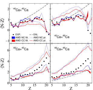
Figure 4: Average neutron excess of the PLF for the experimental data (full circles), filtered AMD-NC and AMD-CC (blue and red continuous curves, respectively). The dashed-dotted line is the EAL from Charity (1998). Results from the QP predicted by the model (before GEMINI++) are plotted in thick red and thin blue dashed lines, respectively.

We first observe that similarly to the experiment (full cirlces), both models (full lines) present an evolution according to the neutron content of the projectile, progressively driven by the evaporative attractor line (EAL, dashed-dotted line extracted from Charity (1998)) with decreasing charge Fable et al. (2022). Concerning the ⁴⁰Ca projectile reactions, we notice a satisfying agreement for both models with the experimental data, except for the most peripheral collisions ($Z=20$) for the neutron-rich target with AMD-CC. Concerning the ⁴⁸Ca projectile reactions, we observe that both models tend to underestimate the neutron-richness of the PLF. This could be ascribed to a too high excitation energy of the QP in both AMD versions, leading to the emission of too many neutrons in the afterburner step. Since model predictions remain too close to the EAL compared to the data, their mutual difference increases with increasing charge. We also note more discrepancies between the models in the $Z_{PLF}=15-20$ peripheral region, AMD-NC predicting values closer to the experiment compared to AMD-CC. Finally, the neutron excess of the associated QP, as predicted by the model (before GEMINI++), is also presented in thin and thick dashed lines for AMD-NC and AMD-CC respectively. We remark that the AMD-NC model exhibits systematically more neutron-rich QP than AMD-CC. The neutron excess is partially preserved for the largest PLF ($Z_{PLF}>15$).

III.3.3 LCP and IMF multiplicities

In addition to the PLF properties, we present in this section the multiplicity of the nuclei measured in coincidence in INDRA. We aim at studying the evolution of cluster emission with the dynamical properties of the reactions, using the parallel velocity $V_{z}^{PLF}$ of the fragment detected in VAMOS as a sorting parameter. Indeed, such a selection allows one to remove the trivial bias induced by the excess of peripheral collisions in AMD-NC, as seen in Fig. 3 in the $V_{z}^{PLF}\simeq 7.5-8$ cm/ns region. For this reason, we focus our interpretations on the semi-peripheral region ($V_{z}^{PLF}\lesssim 7.25$ cm/ns).

Figure 5 shows a comparison of the average total, LCP and IMF multiplicity distributions of the nuclei detected in INDRA as a function of $V_{z}^{PLF}$. We first observe that all multiplicities increase with decreasing $V_{z}^{PLF}$, reflecting an increase of fragment production with increasing dissipation as higher excitation energies are reached on average. Then, we notice that the total multiplicity is governed by the LCP emissions, which both models tend to overproduce for all $V_{z}^{PLF}$. This overproduction increases with decreasing $V_{z}^{PLF}$, reaching about $\Delta\langle M\rangle_{LCP}\simeq 1$ and $\Delta\langle M\rangle_{LCP}\simeq 2$ for neutron-deficient and neutron-rich projectile reactions, respectively, for AMD-NC, while the overproduction remains much smaller for AMD-CC. A noticeable difference is also observed in the IMF multiplicity distributions that present an underproduction in the case of AMD-NC and an overproduction for AMD-CC, more evident for the ⁴⁸Ca target reactions.

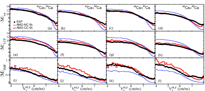
Figure 5: Average total (a-d), LCP (e-h) and IMF (i-l) multiplicity measured with INDRA for the experiment (full circles) and the filterd AMD-NC (thin blue lines) and AMD-CC (thick red lines) simulations followed by GEMINI++.

We present in Figs. 6 and 7 the average multiplicities of $Z=1$ and $Z=2$ nuclei isotopically identified in INDRA as a function of $V_{z}^{PLF}$. The unfiltered neutron distributions are also shown in Fig. 6.

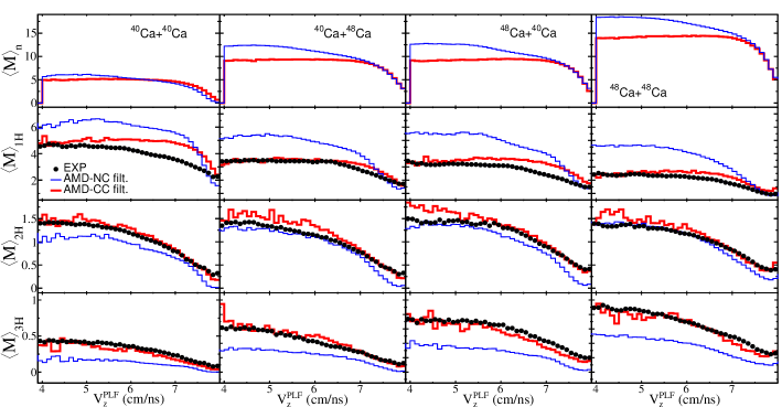
Figure 6: Average multiplicities of neutrons and $Z=1$ nuclei (isotopically identified) for the experiment (full circles) and the filterd AMD-NC (thin blue lines) and AMD-CC (thick red lines) simulations followed by GEMINI++. The neutrons distributions are not filtered.

As a first general comment, we observe that the models exhibit a dominant emission of proton and $\alpha$-particles, similarly to the data. Concerning the $Z=1$ isotopes, we observe an overproduction of protons by AMD-NC, reaching about $\sim 40\%$ for the most dissipative reactions, while AMD-CC present values close to the experimental one at low velocity. Interestingly, an overproduction of neutrons by AMD-NC compared to AMD-CC is also observed for all the systems except the neutron-deficient ⁴⁰Ca$+^{40}$Ca. This indicates that in the case of AMD-NC more free protons (and neutrons) are produced to the detriment of clusters, while the difference in filtered total multiplicity remains reasonable. This seems to be confirmed by the ^2,3H isotopes multiplicities which are systematically underproduced by AMD-NC while the inclusion of cluster formation in AMD-CC leads to a better agreement with the data. Nevertheless, one should exercise caution regarding the ²H isotopes because the SLy4 effective force employed in AMD-CC leads to an overestimation of their binding energy for the soft parametrization, leading to an anomalous increase of their multiplicity Piantelli et al. (2019).

Concerning now the $Z=2$ isotopes, we first notice an underproduction of ³He isotopes from the models, reaching a reduction of about $75\%$ and $50\%$ for AMD-NC and AMD-CC, respectively. The situation is even worse for ⁶He isotope multiplicities, even if the average multiplicities are very small. Finally, a similar behaviour is observed in the case of $\alpha$-particles for both models, without a clear evidence of what model performs the best.

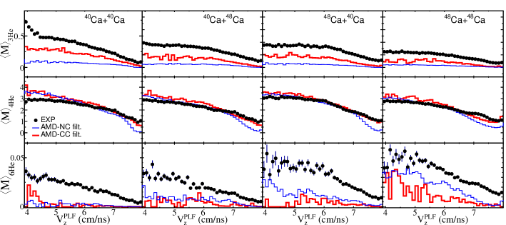
Figure 7: Same as Fig. 6 for $Z=2$ nuclei.

III.3.4 Transverse kinetic energy of LCP

We present in Fig. 8 the distributions of the total transverse energy of the LCP identified in charge, namely $E_{t12}$, extracted from the filtered models and the experiment.

This global variable is of particular interest for centrality estimation in the analysis of isospin transport (see Sec.V) as it is well-suited to the performance of INDRA array for which LCP are detected with a $90\%$ efficiency. It is defined as

$$E_{t12}=\sum_{i:Z_{i}\leq 2}E_{i}\sin^{2}\theta_{i}$$ (1)

where in the sum $i$ runs over the detected (filtered) products of each event with $Z_{i}\leq 2$, laboratory kinetic energy $E_{i}$ and laboratory polar angle $\theta_{i}$.

We first notice in Fig. 8 a good agreement between the experimental distributions (full circles) and the filtered AMD-CC simulations (thick red lines) that reproduce both the experimental trends and $E_{t12}$ values, including the tail of the distributions. In the case of AMD-NC, we observe more narrow-down distributions with higher statistics for the less dissipative collisions ($E_{t12}\lesssim 20$ MeV), as already anticipated from Fig. 3, while the tails of the experimental data are not reproduced. We clearly observe in this figure the relevance of considering clustering to reproduce the experimental kinetic properties of the LCP, as recently evidenced in Frosin et al. (2023).

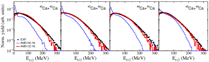
Figure 8: Total transverse kinetic energy distributions of light charged particles (normalized to their integral) for the experiment (full circles) and the filtered AMD-NC (thin blue lines) and AMD-CC (thick red lines) simulations followed by GEMINI++.

III.4 Discussion

As a general comment, we can conclude that both versions of AMD reproduce reasonably well the experimental topology (charge and parallel velocity correlations), highlighting the effect of VAMOS acceptance (and trigger) to favor the measurement of the QP remnant in binary dissipative collisions. A comparison of the filtered simulation impact parameter distributions shows that the data selection criteria have a strong impact on the subset of simulated data from a model to another.

We have shown that the AMD-CC version reproduces remarkably well the experimental velocity, charge and mass distributions of the PLF detected in VAMOS, while a sizable disagreement is obtained with AMD-NC, mostly for the less dissipative collisions. This was anticipated as the AMD-NC version leads to an overproduction of inelastic-like events compared to AMD-CC. Furthermore, a focus on the evolution of the neutron-richness of the PLF shows that both models manage to reproduce, to some extent, the experimental trends. This point is particularly relevant for the study of isospin diffusion, as it is expected to be responsible of such an evolution according to the neutron content of the projectile.

By exploiting the parallel velocity of the PLF as a surrogate for the collision dissipation, we have shown that it is also possible to discuss several aspects of the dynamical emission of clusters. More specifically, comparisons of the average multiplicities have stressed that the inclusion of cluster correlations helps to better reproduce the experimental isotopic multiplicities. A remarkable agreement is obtained for ^1,2,3H isotopes in the case of AMD-CC while AMD-NC tends to overproduce free protons to the detriment of clusters. This is nonetheless less obvious for ^3,4,6He isotopes, as both models tend to underproduce ^3,6He but present a satisfying agreement for ⁴He. It was also shown that AMD-CC tends to better reproduce the average IMF multiplicties.

To conclude, similarly to Piantelli et al. (2017), this work demonstrates that AMD-CC is not only relevant in the study of central collisions, but also for semi-peripheral to peripheral collisions, where binary dissipative collisions exhaust a large part of the total reaction cross section. We also showed that the inclusion of cluster formation is a mandatory step to better reproduce the experimental features, like the multiplicity and transverse kinetic energy distributions. This is particularly interesting in order to improve the comparison protocols used in the study of HIC, as these global observables are used for experimental impact parameter sorting.

IV Impact parameter reconstruction

In this section, we apply a method for impact parameter distribution estimation Das et al. (2018); Rogly et al. (2018), recently adapted from relativistic HIC to the Fermi energy domain by Frankland et. al Frankland et al. (2021). The goal of the method is to infer realistic impact parameters from the inclusive distribution of an experimentally measured observable. Such method is mandatory for suitable comparisons with dynamical models where, as shown in the previous section, we can expect a strong variation in the inclusive impact parameter distribution. More details of the implementation of the method for the INDRA-VAMOS data are given in Appendix A.

We would like to highlight that the software necessary to perform the present analysis is currently implemented in the KaliVeda heavy-ion analysis toolkit Frankland et al. (2023).

IV.1 Validation of the method with AMD-CC

In the following, we present the results of applying the impact parameter reconstruction method presented in Appendix A to the filtered AMD-CC simulated data. Since, as discussed in Section III, AMD-CC reproduces several experimental findings much better than the AMD-NC version, we will now exclusively use and focus on the former. Figure 9 shows an example of the quality of the fits to the inclusive $E_{t12}$ data histograms from AMD-CC stiff, achieved using Eq.3 and the gamma-distribution parametrization. The fit parameters and the reduced $\chi^{2}$ values are given in Table 1 for all simulated data and both parametrizations of the symmetry energy. We observe that the shapes of the filtered distributions are globally well-reproduced by the fits, with a satisfactory goodness-of-fit parameter ($\chi^{2}\sim 1$) and similar parameter values for both parametrizations (for a given system).

Model	System	$\alpha$	$\gamma$	$\theta$	$X_{min}$	$X_{max}$	$\chi^{2}$
				[MeV]	[MeV]	[MeV]
AMD-CC stiff	40Ca$+^{40}$Ca	0.10	0.52	8.95	1	265	1.2
	40Ca$+^{48}$Ca	0.26	0.81	9.42	4	197	1.7
	48Ca$+^{40}$Ca	0.12	0.59	8.68	5	251	1.4
	48Ca$+^{48}$Ca	0.33	0.93	8.48	8	179	1.1
AMD-CC soft	40Ca$+^{40}$Ca	0.15	0.58	7.12	1	246	1.5
	40Ca$+^{48}$Ca	0.31	0.84	9.65	5	187	1.2
	48Ca$+^{40}$Ca	0.15	0.60	8.71	5	241	1.3
	48Ca$+^{48}$Ca	0.35	0.96	9.68	10	175	1.1

Table 1: Model calculations: results of the fits to the total transverse energy. $\chi^{2}$ is the reduced chi-square value of each fit.

Fitting the $P(E_{t12})$ distributions allows to determine the conditional probability distribution $P(E_{t12}|c_{b})$, which is then used to extract the centrality and absolute impact parameter distributions for any sample $\mathbb{S}$ (see Eq.5 and 6).

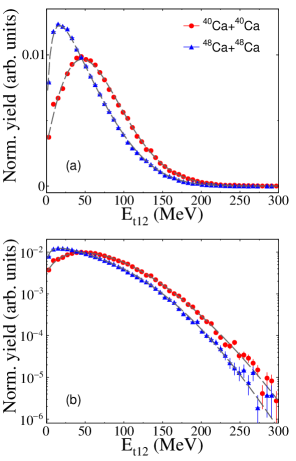
Figure 9: Model calculations: fits (dashed curves) to the inclusive distribution of $E_{t12}$ from AMD-CC (stiff) filtered model predictions (followed by GEMINI++), for the ⁴⁰Ca$+^{40}$Ca and ⁴⁸Ca$+^{48}$Ca reactions. Each distribution is presented in both (a) linear and (b) logarithmic $y$-axes. Statistical uncertainties are not shown when smaller than the symbols.

For this analysis, we have adopted a sampling of 20 bins of $5\%$ experimental centrality $c_{E_{t12}}$. Results for the ⁴⁰Ca$+^{40}$Ca collisions are shown in Fig. 10 for the AMD-CC model followed by GEMINI++ as afterburner, for six centrality intervals. The distributions reconstructed from the deduced form of $P(E_{t12}|c_{b})$ (solid lines) are compared to the actual distributions (filled areas), directly obtained by applying the corresponding cuts in $c_{E_{t12}}$ to the model. Also, the average impact parameter expected to be probed in the most central collisions is about $\langle b\rangle\simeq 3\pm 0.5$ fm, corresponding to semi-central collisions. This limit is mostly induced by VAMOS trigger condition, preventing to measure the most central collisions. Similar results are obtained from AMD-CC with a soft symmetry energy.

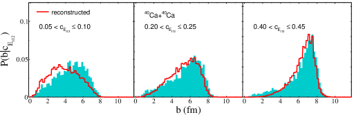
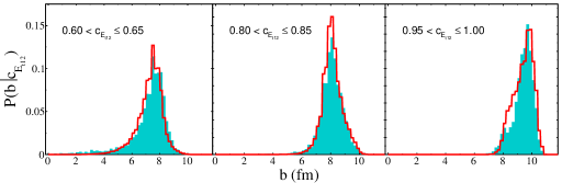
Figure 10: Model calculations: impact parameter probability distributions for various sampling of experimental centrality $c_{E_{t12}}$, returned by the fit (solid lines) and calculated directly (shaded area), for the same ⁴⁰Ca$+^{40}$Ca AMD-CC (stiff) filtered events as in Fig 9.

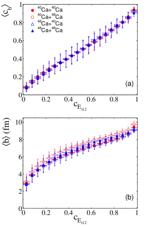
Figure 11: Model calculations: evolution of the average $b$-centrality (a) and impact parameter (b) with the applied sampling of $5\%$ in $c_{E_{t12}}$, for the AMD-CC (stiff) filtered simulations (followed by GEMINI++). The error bars correspond to the standard deviation.

We observe a reasonable agreement between the distributions for all the samplings, with similar results for all the simulated systems. Also, similarly to Frankland et al. (2021), the most central sampling ($0.05<c_{E_{12}}\leq 0.1$) presents a shift that would lead to a slight underestimation of the mean impact parameter.

Finally, we present in Fig. 11 the evolution of the mean centrality $\langle c_{b}\rangle$ and impact parameter $\langle b\rangle$ as a function of the applied sampling in $c_{E_{t12}}$, for all the considered systems. The associated standard deviation are shown as error bars. This plot allows to illustrate the performances of the method to quantitatively characterize the centrality of selected event samples, in a model-independent way (at least for $c_{b}$). We observe a linear correlation between the reconstructed $c_{b}$ and $c_{E_{t12}}$ in the $\langle c_{b}\rangle\simeq 0.05-0.95$ range, independently of the system. This evolution is not observed for the reconstructed $b$, where values present a system-dependence and increase non-linearly from $\langle b\rangle\simeq 3$ fm to $\langle b\rangle\simeq 9$ fm.

IV.2 Application to the experimental data

Following the same procedure as in the previous section, we can estimate the impact parameter distributions for the experimental data. Figure 12 shows an example of the quality of the fits to the inclusive $E_{t12}$ experimental data, achieved using Eq.3 and the gamma-distribution parametrization, similarly to Fig. 9. The fit parameters and the reduced $\chi^{2}$ values are given in Table 2 for the four systems under study.

System	$\alpha$	$\gamma$	$\theta$	$X_{min}$	$X_{max}$	$\chi^{2}$
			[MeV]	[MeV]	[MeV]
40Ca$+^{40}$Ca	0.14	0.69	10.29	4	278	1.3
40Ca$+^{48}$Ca	0.37	0.82	12.90	7	167	1.3
48Ca$+^{40}$Ca	0.17	0.71	9.11	6	257	1.1
48Ca$+^{48}$Ca	0.10	0.55	13.01	1	233	1.4

Table 2: Experimental data: results of the fits to the total transverse energy. $\chi^{2}$ is the reduced chi-square value of each fit.

The centrality and absolute impact parameter distributions for all the samples in experimental centrality $c_{E_{t12}}$ are then estimated using Eqs. 5 and 6, respectively.

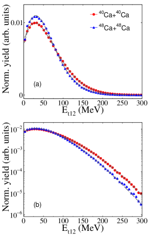
Figure 12: Experimental data: fits (dashed curves) to the inclusive distribution of $E_{t12}$ for the ⁴⁰Ca$+^{40}$Ca and ⁴⁸Ca$+^{48}$Ca reactions. Each distribution is presented in both (a) linear and (b) logarithmic $y$-axes. Statistical uncertainties are not shown when smaller than the symbols.

The evolution of the average centrality $\langle c_{b}\rangle$ and impact parameter $\langle b\rangle$ as a function of $c_{E_{t12}}$ are presented in Fig. 13(a) and (b), respectively, for the four reactions under study. For both observables we find, as expected, increasing values with increasing $c_{E_{t12}}$, even if a stronger system-dependence than the model is observed for $\langle b\rangle$. Concerning $\langle b\rangle$, we have used the inclusive impact parameter of the filtered model (after data selection criteria) as a surrogate for $P(b)$ in Eq.6, similarly to Sec. IV.1. The plots given in Fig. 13(b) are thus obtained with the inclusive impact parameter distributions extracted from the filtered AMD-CC with a stiff symmetry energy. It was verified that the same quantitative results are obtained with the soft symmetry energy (within the error bars), as the $P(b)$ distributions are almost not sensitive to the employed parametrization.

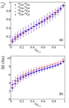
Figure 13: Experimental data: evolution of the average $b$-centrality (a) and impact parameter (b) with the applied sampling of $5\%$ in $c_{E_{t12}}$. The error bars correspond to the standard deviation.

V Isospin diffusion

This section is dedicated to the study of isospin diffusion from the quasiprojectile (QP) and its remnant (PLF), defined as the fragment measured in VAMOS. The isospin transport ratio, described in the following, is used to quantify the degree of isospin equilibration, while its evolution is followed as a function of the centrality or impact parameter, estimated using the method described in Sec.IV. In the first part, we focus on the AMD-CC model, in order to characterize the effect of the impact parameter reconstruction on the isospin equilibration measured from the QP along with the effect of sequential decays. In the continuity with our previous works Fable et al. (2022, 2023), the experimental method applied to reconstruct the primary QP fragments, including the estimation of evaporated neutrons, is also tested and compared to the result obtained from the actual QP predicted by the model. Details about the method are given in Appendix B. In the second part, the same protocol will be applied to the experimental data, allowing direct comparisons with the model.

V.1 Isospin transport ratio

The isospin transport ratio (also called imbalance ratio) was introduced by Rami et. al to deduce quantitative signals of isospin diffusion in experimental data Rami et al. (2000). It consists of combining an isospin-sensitive observable measured, under the same experimental conditions, with four systems differing in their initial neutron-to-proton ratio. It is defined as

$$R_{x}=\frac{2x^{M}-x^{NR}-x^{ND}}{x^{NR}-x^{ND}}$$ (2)

where $x$ is an isospin-sensitive observable expected to be univocally related to the $N/Z$ of the systems under study, measured for the symmetric neutron-rich (NR) and neutron-deficient (ND) reactions, while the two mixed reactions (M) reach a neutron content in between these two references. The evolution of $R_{x}$ towards $N/Z$ equilibration is thus followed as a function of a centrality parameter correlated to the dissipation of the collision. By construction, $R_{x}=\pm 1$, in the limit of fully non-equilibrated conditions (isospin transparency), while equilibration is generally signaled by both mixed reactions reaching the same value of the ratio.

V.2 Isospin diffusion in AMD-CC

We present in Fig. 14(a) and (b) the evolution of the asymmetry $\delta=(N-Z)/A$ as a function of the centrality $c_{E_{t12}}$ from AMD-CC (stiff) followed by GEMINI++ for the PLF and the reconstructed QP, respectively. The same sampling as the one used for the impact parameter estimation has been used (20 bins of $5\%$ in $c_{E_{t12}}$).

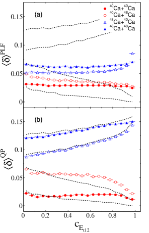
Figure 14: Model calculations: distribution of the average asymmetry $\delta$ as a function of the centrality $c_{E_{t12}}$ for (a) the PLF and (b) the reconstructed QP, for AMD-CC (stiff) filtered simulations (followed by GEMINI++). The dashed lines correspond to the QP predicted by the filtered model before GEMINI++. Statistical error bars are smaller than the symbols.

We first observe that both the PLF and the reconstructed QP exhibit the same hierarchy according to the neutron-richness of the projectile and, to a lesser extent, of the target, as observed in the experimental data Fable et al. (2023). The latter is also observed for the QP predicted by the model, represented in dashed line for each reaction. Nonetheless, the model exhibits for all systems a significant difference between the asymmetry values obtained for the QP and its residue, resulting from the effect of sequential decays Ogul et al. (2023), that seems to be restored by the QP reconstruction method for ⁴⁸Ca projectile reactions but not for ⁴⁰Ca.

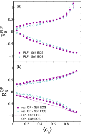
Figure 15: Model calculations: isospin transport ratio as a function of the estimated average $\langle c_{b}\rangle$ for the PLF (a) and the reconstructed QP (b), respectively, from the AMD-CC model with a stiff (full squares) and a soft (open circles) parametrization. Results with the QP predicted by the model are superimposed in dashed lines.

Using the estimated $\langle c_{b}\rangle$ and asymmetry $\delta$ for each sampling in $c_{E_{t12}}$, presented in Figs. 11(a) and 14 respectively, the corresponding isospin transport ratio can be computed from Eq.2 and plotted as a function of $\langle c_{b}\rangle$. The results are presented in Fig. 15 (a) and (b) for the PLF and the QP, respectively, for the stiff and soft parametrization. First, we observe converging values of the isospin transport ratio when moving from peripheral collisions (high $\langle c_{b}\rangle$ values) to more central collisions (low $\langle c_{b}\rangle$ values), indicating that an evolution towards isospin equilibration is predicted by the AMD-CC model. Second, we notice that for the most central collisions probed ($\langle c_{b}\rangle<0.1$) the full equilibration condition is not reached. As observed in Fig. 11(b), the average impact parameter expected to be probed in this reagion of centrality is about $\langle b\rangle\simeq 3\pm 0.5$ fm, corresponding to semi-central collisions. Third, the results indicate a weak sensitivity of the isospin transport ratio to the stiffness of the employed symmetry energy within the model, for both the PLF and the reconstructed QP. Indeed, we notice that for the stiff asymmetry term (close squares), $R_{\delta}$ exhibits systematically less isospin equilibration compared to the soft asymmetry term (open circles), for both the PLF and the reconstructed QP. This is also observed from the QP predicted by the filtered model (not reconstructed), superimposed in thin and thick dashed lines for the soft and stiff parametrization, respectively. Such behaviour has already been mentioned in Tsang et al. (2004) and Colonna, Maria et al. (2014) with BUU and SMF calculations, respectively.

In a similar way, the evolution of the isospin transport ratio as a function of the average reduced impact parameter, namely $\langle b\rangle/b_{gr}$, can be extracted from Figs. 11(b) and 14. The results are presented in Fig. 16 (a) and (b) for the PLF and the QP, respectively, for the stiff and soft parametrizations. We observe that the same conclusion as the one from Fig. 15 can be drawn, at least in the $\langle b\rangle/b_{gr}>0.3$ region. It is worth noting that the sensitivity to the stiffness of the employed symmetry energy remains weak, independently of the centrality or the QP reconstruction.

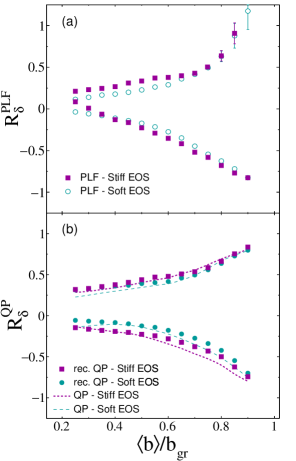
Figure 16: Model calculations: isospin transport ratio as a function of the estimated average reduced impact parameter $\langle b\rangle/b_{gr}$ for the PLF (a) and the reconstructed QP (b), respectively, from the AMD-CC model with a stiff (squares) and a soft (circles) parametrization. Error bars are not shown when smaller than the symbols. Results with the QP predicted by the model are shown in dashed lines.

V.3 Isospin diffusion in experimental data

In this Section, we apply the same protocol used with the AMD-CC model to the INDRA-VAMOS experimental data.

Concerning the evaporated neutron estimation, the mean neutron multiplicities extracted from filtered AMD-CC followed by GEMINI++ calculations were used as a surrogate. More precisely, a constant scaling factor $\langle k\rangle=0.8$ is applied to the model neutron distribution in order to take into account the overstimation of light particles observed with AMD-CC (see Sec.III.3.3). More details are given in Appendix B.

We present in Figs. 17(a) and (b) the evolution of the experimental asymmetry $\delta$ as a function of the centrality $c_{E_{t12}}$ (with a sampling of $5\%$) for the PLF and the reconstructed QP, respectively.

Concerning the PLF, we notice that the experimental data (symbols) exhibit systematically higher asymmetry values than AMD-CC (dashed lines), while the same hierarchy is obtained. This effect is even more remarkable for the ⁴⁸Ca projectile reactions, leading to the conclusion that AMD-CC (followed by GEMINI++) fails to reproduce the experimental QP remnant neutron-enrichment over the full $c_{E_{t12}}$ domain. Our results are consistent with the analysis of ^40,48Ca+⁴⁰Ca reactions performed with four blocks of FAZIA, reported in (Camaiani et al., 2021). Concerning the reconstructed QP, we observe that the applied reconstruction method leads to a better agreement between the experimental data and the model, except for the ⁴⁰Ca$+^{48}$Ca asymmetric reaction.

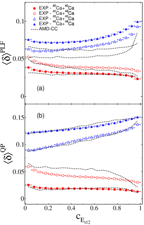
Figure 17: Experimental data : distribution of the average asymmetry $\delta$ as a function of the centrality $c_{E_{t12}}$ for (a) the PLF and (b) the reconstructed QP. The dashed lines correspond to (a) the PLF and (b) the reconstructed QP obtained from AMD-CC (stiff) filtered simulations (followed by GEMINI++). Statistical error bars are smaller than the symbols.

Based on the results presented in Figs. 13(b) and 17, the experimental isospin transport ratio was computed from Eq.2 as a function of the estimated reduced impact parameter $\langle b\rangle/b_{gr}$. For more consistency, the scaling factor $k$ used for the evaporated neutron estimation was varied from $k=0.7-0.9$, corresponding to a variation of one standard deviation of the average neutron multiplicity obtained for $\langle k\rangle=0.8$, while the results presented thereafter are averaged over this domain in $k$. The difference in average neutron multiplicity induced by the variation of $k$ is larger than the one induced by the stiffness of the symmetry energy. Thus, this average also allows to remove the dependence of the average neutron multiplicity on the employed stiffness for the experimental QP reconstruction.

The results are presented in Figs. 18 (a) and (b) for the experimental PLF and reconstructed QP (full circles), respectively. It must also be noted that similar results can be drawn from the evolution of the experimental $R_{\delta}$ with $\langle c_{b}\rangle$. For both PLF and reconstructed QP, we first observe an evolution of the isospin transport ratio towards isospin equilibration, with decreasing values from about $R_{\delta}\simeq\pm 0.75$ towards $R_{\delta}\simeq-0.1$ and $R_{\delta}\simeq 0.3$ for the neutron-deficient and neutron-rich mixed reactions, respectively, when moving from the most peripheral ($\langle b\rangle/b_{gr}\simeq 0.9$) to the most central ($\langle b\rangle/b_{gr}\simeq 0.3$) measured collisions. Furthermore, we remark a noticable difference between the slopes of the ratios obtained from the two mixed reactions, leading to experimental values closer to the AMD-CC stiff distributions for the ⁴⁸Ca$+^{40}$Ca as mixed system, while the PLF presents more equilibration than the QP at small impact parameters, consistently with the model (open symbols). It is worth noting that a similar experimental trend is obtained for the PLF with ⁴⁸Ca+⁴⁰Ca mixed reaction in (Camaiani et al., 2021), where it was concluded that the observed discrepancy can be ascribed to an overestimated probability of nucleon transfer in AMD. In our understanding, the larger model-experiment discrepancy of $R_{\delta}$ in ⁴⁰Ca$+^{48}$Ca reaction originates from the significant difference in the evolution of the asymmetry $\delta$ with centrality $c_{E_{t12}}$, as observed in Fig. 17.

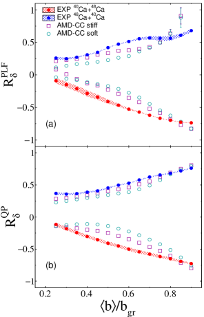
Figure 18: Experimental isospin transport ratio computed from the asymmetry $\delta$ for the average reduced impact parameter $\langle b\rangle/b_{gr}$ estimated from the method described in Sec.IV, for (a) the PLF and (b) the reconstructed QP. Open symbols represent the AMD-CC filtered simulations (followed by GEMINI++) for a stiff (open squares) and a soft (open circles) symmetry energy.

VI Summary and conclusions

In this work, we have presented an investigation of isospin diffusion in ^40,48Ca$+^{40,48}$Ca reactions at 35 MeV/nucleon, by comparing INDRA-VAMOS experimental data to the output of the filtered AMD model followed by GEMINI++ as afterburner.

Two versions of AMD, with and without cluster correlations, were employed in order to study the role of clustering in the global observables in the measured reactions. Generally, both versions reproduce the experimental topology (charge and parallel velocity correlation). Nonetheless, it was shown that the inclusion of clusters allows to better reproduce the characteristics (velocity, mass and charge distributions) of the QP remnant detected in VAMOS (PLF). Furthermore, comparisons of the average multiplicities have evidenced that clustering allows to better reproduce the experimental multiplicities while the latter is mandatory to reproduce the LCP transverse kinetic energy distributions. It is also important to note that, aside from clustering, the treatment of dissipation (collision term), nuclear stopping and excitation energy within the models plays an important role in reproducing the experimental data. We believe that reproducing the global observables outlined in this study sets a fundamental standard for the trustworthiness of dynamic models. Such standard ensures that, when comparing them to experimental data, the comparison becomes meaningful and enhances the precision in constraining the equation of state of nuclear matter.

We have applied a method for impact parameter reconstruction specifically adapted to the Fermi energy domain, allowing to infer information on the centrality (and the impact parameter) from the inclusive distribution of an experimentally measured observable. The method was adapted to INDRA-VAMOS, using the inclusive distribution of total transverse kinetic energy, and tested within the AMD-CC model, proving its relevance over the whole impact parameter domain.

The isospin diffusion phenomenon was investigated by means of the isospin transport ratio computed from the asymmetry $\delta=(N-Z)/A$ of both PLF and reconstructed QP. For the first time, we have highlighted that the employed impact parameter reconstruction method allows a more direct comparison to the experimental data for the study of isospin diffusion. Furthermore, our results show that the weak sensitivity of the isospin transport ratio to the stiffness of the employed symmetry energy, expected for the QP predicted by the model (before sequential decays), holds for both the PLF and the reconstructed QP. Nonetheless, a noticable disagreement is observed in the centrality dependence of the ratios between the experimental data and the model, more specifically for the ⁴⁰Ca$+^{48}$Ca mixed system. Such difference can be anticipated from the individual evolution of $\delta$ with centrality obtained from the PLF, that the AMD model followed by GEMINI++ fails to reproduce for all reactions. Interestingly, the reconstruction of the QP indicates a better agreement between the model and the experimental data for the neutron rich ⁴⁸Ca reactions. The evolution of the average neutron excess obtained from the filtered QP also indicates that, even if the clusters are considered, the ⁴⁸Ca reactions are mostly driven by the Evaporative Attractor Line as compared to the ⁴⁰Ca projectile reactions.

The results presented in this work constitute a further step to improve the comparison protocol employed in the study of isospin transport and of the nuclear EoS. The subsequent phase involves implementing the suggested protocol across a variety of dynamical models, including both QMD-like and BUU-like formalisms, for which we can anticipate that variations in the Mean-Field implementation will result in distinct behaviors in the isospin transport ratio. This work is currently in progress.

Appendix A Impact parameter reconstruction

A.1 Method

By definition, the inclusive distribution of an observable $X$, $P(X)$, resulting from all measured collisions with an unknown impact parameter distribution $P(b)$, is related to the conditional probability distribution of $X$ at fixed $b$, $P(X|b)$, such as

$$P(X)\equiv\int_{0}^{+\infty}P(b)P(X|b)db=\int_{0}^{1}P(X|c_{b})dc_{b}$$ (3)

The right hand side of Eq.3 is obtained by introducing the centrality $c_{b}$, defined as the cumulative distribution function of $P(b)$:

$$c_{b}\equiv\int_{0}^{b}P(b^{\prime})db^{\prime}$$ (4)

with $P(c_{b})=1$ $\forall c_{b}$. As described in Rogly et al. (2018); Frankland et al. (2021), Eq.3 can be used to determine $P(X|c_{b})$ by fitting the experimentally measured inclusive distribution $P(X)$, with a suitable probability density function (p.d.f) which encodes both the centrality dependence of the mean value $\overline{X}(c_{b})$ and the fluctuation of $X$ about this mean value.

Once $P(X|c_{b})$ is obtained by fitting the experimental $P(X)$ distribution, the centrality distribution of any experimental generic sample $\mathbb{S}$, $P(c_{b}|\mathbb{S})$, can be deduced from the Bayes’ theorem:

$$P(c_{b}|\mathbb{S})=\frac{\int P(X|c_{b})\frac{P(X|\mathbb{S})}{P(X)}dX}{\int P(X|\mathbb{S})dX}$$ (5)

where $P(X|\mathbb{S})$ is an histogram of $X$ filled with the events of the sample while the integrals are performed over the full domain of $X$.

Finally, the absolute impact parameter distribution can be deduced from the previously calculated centrality distribution, such as

$$P(b|\mathbb{S})=P(b)P(c_{b}(b)|\mathbb{S})$$ (6)

The method described above is model-independent and allows to take into account the fluctuations inherent to the relationship between any experimental observable and the impact parameter. It should nonetheless be noted that it is necessary to assume a specific form for $P(b)$ in order to use Eq.5 and calculate $c_{b}(b)$, i.e. the relation between $c_{b}$ and $b$.

A.2 Implementation for INDRA-VAMOS data

In the present analysis the impact parameter distributions are reconstructed by using the inclusive distributions in total transverse energy of the LCP, namely $P(E_{t12})$, where $E_{t12}$ is defined in Eq.1. It is worth noting that the PLF properties are largely independent of this quantity, avoiding possible trivial bias due to auto-correlation with the event sorting for the study of the isospin transport ratio Rami et al. (2000). Also, as it can be seen in Fig. 8, this quantity is relatively well reproduced by the AMD-CC filtered model while we have verified that it presents a monotonic relationship with centrality $c_{b}$ within the model.

Secondly, the data are sampled according to the experimental centrality $c_{E_{t12}}$, defined as the complementary cumulative distribution function of the $P(E_{t12})$ distribution:

$$c_{E_{t12}}\equiv\int_{E_{t12}}^{+\infty}P(\tilde{E}_{t12})\>\mathrm{d}\tilde{E}_{t12}$$ (7)

By construction, $c_{E_{t12}}$ decreases from 1 to 0 as $E_{t12}$ goes from its minimum ($\sim 0$) to its (system-dependent) maximum value. Therefore, large ($\sim 1$) $c_{E_{t12}}$ values are associated with the most peripheral collisions while smaller values ($c_{E_{t12}}\rightarrow 0$) indicate smaller average impact parameters. This choice is based on our previous work and aims to remove the system-dependence of the $E_{t12}$ distributions in the data sampling Fable et al. (2023). Indeed, since bins of fixed width of $c_{E_{t12}}$ contain the same number of events, we expect them to have the same statistical significance, whatever the centrality. Based on the aforementioned considerations, a fixed step of $5\%$ experimental centrality $c_{E_{t12}}$ have been used for the data sampling, for a total of 20 bin samples.

Thirdly, we have adopted the same specific implementation as Frankland et. al for the fluctuation kernel and the centrality dependence of $\overline{E}_{t12}$. Concerning the fluctuation kernel, since $E_{t12}$ is positive the gamma-distribution is an ideal choice Rogly et al. (2018). Accordingly, the p.d.f used to fit the inclusive distribution reads:

$$P(X|c_{b})=\frac{1}{\Gamma(k)\theta^{k}}X^{k-1}e^{-X/\theta}$$ (8)

where $k$ and $\theta$ are two positive parameters related to the mean value $\overline{X}$ and its variance, respectively. As pointed out in Rogly et al. (2018), these parameters generally depend on the centrality, while the fit to the inclusive distribution $P(X)$ using Eq.8 to extract $k(c_{b})$ and $\theta(c_{b})$ is underconstrained. In the framework of the gamma-distribution of Eq.8, the centrality dependence of $k$ must be parametrized, and it is generally assumed that the variance parameter $\theta$ is constant for all centralities. Therefore, similarly to Frankland et al. (2021), in this work $k$ is parametrized with a monotonically decreasing function of centrality, while $\theta$ is a free parameter of the fit constrained by the tail of $P(X)$. In summary, 5 free parameters $(\alpha,\gamma,\theta,X_{min},X_{max})$ are required for the fit, which are explicitly defined in Frankland et al. (2021).

Finally, we would like to stress that if the model calculations were run with a geometric impact parameter distribution, the filtered impact parameter distribution $P(b)$ can not be well-fitted by the usual approximation observed for most of the INDRA dataset (see Eq.12 in Frankland et al. (2021)). This can be seen in Fig. 2, where we clearly observe the effect of the VAMOS angular cuts that favor the detection of semi-peripheral and peripheral events, even for AMD-CC, in the $b/b_{gr}=0.6-0.9$ region. For this reason, and at the cost of losing the model independence for $P(X|\mathbb{S})$, we have used the inclusive impact parameter distribution directly obtained from the filtered model as a surrogate for $P(b)$ in Eq.6. Therefore, for more consistency the results on isospin diffusion will be presented using both Eqs.5 and 6, keeping in mind that the former is model-independent.

Appendix B Quasiprojectile reconstruction

Similarly to our previous works, the relative velocities between the reactions products measured (filtered) in INDRA and (i) the PLF detected (filtered) in VAMOS and (ii) the fragment with the largest identified charge at backward angles (supposed to be the TLF) are calculated. Numerically, cuts on the associated relative velocities, respectively $V_{rel,PLF}$ and $V_{rel,TLF}$, were applied in order to include fragments whose velocities verify $\frac{V_{rel,TLF}}{V_{rel,PLF}}>1.35$ for $Z=1$ and $\frac{V_{rel,TLF}}{V_{rel,PLF}}>1.75$ for $Z\geq 2$. The values of the cut-off thresholds were estimated from both AMD-NC and AMD-CC filtered simulations, to optimize the contribution of the actual QP to the reconstruction. Interestingly, the values of the cuts are similar for both versions of AMD, while their effect remains consistent for the models and the experiment.

The quasiprojectile atomic number $Z_{QP}$ reads

$$Z_{QP}=Z_{PLF}+\sum_{i}^{M_{I}}Z_{i}$$ (9)

where $Z_{PLF}$ is the charge of the fragment measured (filtered) in VAMOS and the sum runs over the charge $Z_{i}$ of the $M_{I}$ selected particles.

Similarly, the quasiprojectile mass number (without evaporated neutron contribution) $\tilde{A}_{QP}$ reads

$$\tilde{A}_{QP}=A_{PLF}+\sum_{i}^{M_{I}}A_{i}$$ (10)

where $A_{PLF}$ is the mass of the fragment in VAMOS and the sum runs over the mass $A_{i}$ of the $M_{I}$ selected particles.

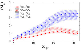
Figure 19: Average neutron multiplicities distributions used for the mass reconstruction of the experimental quasiprojectile as a function of its charge. The symbols correspond to the values obtained for $\langle k\rangle=0.8$ while the dashed areas represent a variation of $k=0.7-0.9$ (roughly one standard deviation).

As the neutrons were not measured in the INDRA-VAMOS experiment, the distributions of the neutrons evaporated by the reconstructed QP from the AMD filtered model calculations were used as a substitute. More precisely, for each event with reconstructed charge $Z_{QP}$ and mass without the neutron $\tilde{A}_{QP}$, the evaporated neutron multiplicity was estimated from a random number generator following the filtered model neutron multiplicity distribution (histogram).

The estimated evaporated neutron multiplicity is thus the following:

$$M_{n}(Z_{QP},\tilde{A}_{QP})=\lceil M_{n}^{rdm}(Z_{QP},\tilde{A}_{QP})\cdot k\rceil$$ (11)

where $M_{n}^{rdm}$ is the random neutron multiplicity extracted from the model histogram, $k$ is a correction factor and $\lceil\rceil$ is the ceiling function.

The scaling factor $k$ is intended to correct from the fact that both AMD models tends to overestimate the proton multiplicities compared to the experiment, as observed in Sec.III.3.3.

Thus, assuming that the experimental and filtered model average neutron-to-proton multiplicity ratios are equivalent, we have:

$$\langle M_{n}\rangle^{exp}=\langle M_{n}\rangle^{mod}\cdot\frac{\langle M_{p}\rangle^{exp}}{\langle M_{p}\rangle^{mod}}=\langle M_{n}\rangle^{mod}\cdot k$$ (12)

where $\langle M_{n,p}\rangle^{exp,mod}$ are the neutron and proton average multiplicities of the experiment and model, respectively.

Therefore, $k=1$ when applying the evaporated neutron correction within the model, while a constant value of $\langle k\rangle=0.8$ is applied in the case of the experiment, which corresponds to the average scaling factor over all systems and charges. The resulting experimental average neutron distributions are presented in Fig. 19, for the four systems under study. In this figure, the symbols correspond to the values obtained for $\langle k\rangle=0.8$, while the dashed areas represent a variation from $k=0.7-0.9$, corresponding to a variation of one standard deviation.

References

- Lattimer and Prakash (2016) J. M. Lattimer and M. Prakash, Physics Reports 621, 127 (2016), ISSN 0370-1573, memorial Volume in Honor of Gerald E. Brown.
- Toro et al. (2010) M. D. Toro, V. Baran, M. Colonna, and V. Greco, Journal of Physics G: Nuclear and Particle Physics 37, 083101 (2010), URL https://dx.doi.org/10.1088/0954-3899/37/8/083101.
- Tsang et al. (2012) M. B. Tsang, J. R. Stone, F. Camera, P. Danielewicz, S. Gandolfi, K. Hebeler, C. J. Horowitz, J. Lee, W. G. Lynch, Z. Kohley, et al., Phys. Rev. C 86, 015803 (2012), URL https://link.aps.org/doi/10.1103/PhysRevC.86.015803.
- Lattimer and Lim (2013) J. M. Lattimer and Y. Lim, The Astrophysical Journal 771, 51 (2013), URL https://dx.doi.org/10.1088/0004-637X/771/1/51.
- Huth et al. (2022) S. Huth, P. T. H. Pang, I. Tews, T. Dietrich, A. Le Fèvre, A. Schwenk, W. Trautmann, K. Agarwal, M. Bulla, M. W. Coughlin, et al., Nature 606, 276 (2022), ISSN 1476-4687.
- Lynch and Tsang (2022) W. Lynch and M. Tsang, Physics Letters B 830, 137098 (2022), ISSN 0370-2693, URL https://www.sciencedirect.com/science/article/pii/S0370269322002325.
- Russotto et al. (2011) P. Russotto, P. Wu, M. Zoric, M. Chartier, Y. Leifels, R. Lemmon, Q. Li, J. Łukasik, A. Pagano, P. Pawłowski, et al., Physics Letters B 697, 471 (2011), ISSN 0370-2693, URL https://www.sciencedirect.com/science/article/pii/S037026931100178X.
- Abbott et al. (2017) B. P. Abbott, R. Abbott, T. D. Abbott, F. Acernese, K. Ackley, C. Adams, T. Adams, P. Addesso, R. X. Adhikari, V. B. Adya, et al., Phys. Rev. Lett. 119, 161101 (2017).
- Typel (2013) S. Typel, Journal of Physics: Conference Series 420, 012078 (2013), URL https://dx.doi.org/10.1088/1742-6596/420/1/012078.
- Brown (2013) B. A. Brown, Phys. Rev. Lett. 111, 232502 (2013), URL https://link.aps.org/doi/10.1103/PhysRevLett.111.232502.
- Danielewicz and Lee (2014) P. Danielewicz and J. Lee, Nuclear Physics A 922, 1 (2014), ISSN 0375-9474, URL https://www.sciencedirect.com/science/article/pii/S0375947413007872.
- Russotto et al. (2016) P. Russotto, S. Gannon, S. Kupny, P. Lasko, L. Acosta, M. Adamczyk, A. Al-Ajlan, M. Al-Garawi, S. Al-Homaidhi, F. Amorini, et al., Phys. Rev. C 94, 034608 (2016), URL https://link.aps.org/doi/10.1103/PhysRevC.94.034608.
- Estee et al. (2021) J. Estee, W. G. Lynch, C. Y. Tsang, J. Barney, G. Jhang, M. B. Tsang, R. Wang, M. Kaneko, J. W. Lee, T. Isobe, et al. ( Collaboration), Phys. Rev. Lett. 126, 162701 (2021), URL https://link.aps.org/doi/10.1103/PhysRevLett.126.162701.
- Tsang et al. (2009a) M. B. Tsang, Y. Zhang, P. Danielewicz, M. Famiano, Z. Li, W. G. Lynch, and A. W. Steiner, Phys. Rev. Lett. 102, 122701 (2009a), URL https://link.aps.org/doi/10.1103/PhysRevLett.102.122701.
- Tsang et al. (2009b) M. B. Tsang, Y. Zhang, P. Danielewicz, M. Famiano, Z. Li, W. G. Lynch, and A. W. Steiner, Phys. Rev. Lett. 102, 122701 (2009b).
- Rami et al. (2000) F. Rami, Y. Leifels, B. de Schauenburg, A. Gobbi, B. Hong, J. P. Alard, A. Andronic, R. Averbeck, V. Barret, Z. Basrak, et al., Phys. Rev. Lett. 84, 1120 (2000).
- Camaiani et al. (2020) A. Camaiani, S. Piantelli, A. Ono, G. Casini, B. Borderie, R. Bougault, C. Ciampi, J. A. Dueñas, C. Frosin, J. D. Frankland, et al., Phys. Rev. C 102, 044607 (2020), URL https://link.aps.org/doi/10.1103/PhysRevC.102.044607.
- Camaiani et al. (2021) A. Camaiani, G. Casini, S. Piantelli, A. Ono, E. Bonnet, R. Alba, S. Barlini, B. Borderie, R. Bougault, C. Ciampi, et al., Phys. Rev. C 103, 014605 (2021), URL https://link.aps.org/doi/10.1103/PhysRevC.103.014605.
- Piantelli et al. (2021) S. Piantelli, G. Casini, A. Ono, G. Poggi, G. Pastore, S. Barlini, M. Bini, A. Boiano, E. Bonnet, B. Borderie, et al. (FAZIA Collaboration), Phys. Rev. C 103, 014603 (2021), URL https://link.aps.org/doi/10.1103/PhysRevC.103.014603.
- Ciampi et al. (2022) C. Ciampi, S. Piantelli, G. Casini, G. Pasquali, J. Quicray, L. Baldesi, S. Barlini, B. Borderie, R. Bougault, A. Camaiani, et al., Phys. Rev. C 106, 024603 (2022).
- Fable et al. (2023) Q. Fable, A. Chbihi, J. D. Frankland, P. Napolitani, G. Verde, E. Bonnet, B. Borderie, R. Bougault, E. Galichet, T. Génard, et al. (INDRA Collaboration), Phys. Rev. C 107, 014604 (2023), URL https://link.aps.org/doi/10.1103/PhysRevC.107.014604.
- Pouthas et al. (1995) J. Pouthas, B. Borderie, R. Dayras, E. Plagnol, M. F. Rivet, F. Saint-Laurent, J. C. Steckmeyer, G. Auger, C. O. Bacri, S. Barbey, et al., Nucl. Instr. and Meth. in Phys. Res. A 357, 418 (1995).
- Pouthas et al. (1996) J. Pouthas, A. Bertaut, B. Borderie, P. Bourgault, B. Cahan, G. Carles, D. Charlet, D. Cussol, R. Dayras, M. Engrand, et al., Nucl. Instr. and Meth. in Phys. Res. A 369, 222 (1996).
- Pullanhiotan et al. (2008) S. Pullanhiotan, M. Rejmund, A. Navin, W. Mittig, and S. Bhattacharyya, Nuclear Instruments and Methods in Physics Research Section A: Accelerators, Spectrometers, Detectors and Associated Equipment 593, 343 (2008), ISSN 0168-9002, URL https://www.sciencedirect.com/science/article/pii/S0168900208007080.
- Lemasson and Rejmund (2023) A. Lemasson and M. Rejmund, Nuclear Instruments and Methods in Physics Research Section A: Accelerators, Spectrometers, Detectors and Associated Equipment 1054, 168407 (2023), ISSN 0168-9002, URL https://www.sciencedirect.com/science/article/pii/S0168900223003972.
- Fable et al. (2022) Q. Fable, A. Chbihi, M. Boisjoli, J. D. Frankland, A. Le Fèvre, N. Le Neindre, P. Marini, G. Verde, G. Ademard, L. Bardelli, et al., Phys. Rev. C 106, 024605 (2022).
- Ono et al. (1992) A. Ono, H. Horiuchi, T. Maruyama, and A. Ohnishi, Progress of Theoretical Physics 87, 1185 (1992), ISSN 0033-068X, eprint https://academic.oup.com/ptp/article-pdf/87/5/1185/5272175/87-5-1185.pdf, URL https://doi.org/10.1143/ptp/87.5.1185.
- Kanada-En’yo et al. (2003) Y. Kanada-En’yo, M. Kimura, and H. Horiuchi, Comptes Rendus Physique 4, 497 (2003), ISSN 1631-0705, URL https://www.sciencedirect.com/science/article/pii/S1631070503000628.
- Ono (2013) A. Ono, Journal of Physics: Conference Series 420, 012103 (2013), URL https://dx.doi.org/10.1088/1742-6596/420/1/012103.
- Wolter et al. (2022) H. Wolter, M. Colonna, D. Cozma, P. Danielewicz, C. M. Ko, R. Kumar, A. Ono, M. B. Tsang, J. Xu, Y.-X. Zhang, et al., Progress in Particle and Nuclear Physics 125, 103962 (2022), ISSN 0146-6410, URL https://www.sciencedirect.com/science/article/pii/S0146641022000230.
- Frosin et al. (2023) C. Frosin, S. Piantelli, G. Casini, A. Ono, A. Camaiani, L. Baldesi, S. Barlini, B. Borderie, R. Bougault, C. Ciampi, et al. (INDRA-FAZIA Collaboration), Phys. Rev. C 107, 044614 (2023), URL https://link.aps.org/doi/10.1103/PhysRevC.107.044614.
- Piantelli et al. (2017) S. Piantelli, S. Valdré, S. Barlini, G. Casini, M. Colonna, G. Baiocco, M. Bini, M. Bruno, A. Camaiani, S. Carboni, et al., Phys. Rev. C 96, 034622 (2017), URL https://link.aps.org/doi/10.1103/PhysRevC.96.034622.
- Ono (2019) A. Ono, Progress in Particle and Nuclear Physics 105, 139 (2019), ISSN 0146-6410, URL https://www.sciencedirect.com/science/article/pii/S0146641018300863.
- Ono (1999) A. Ono, Phys. Rev. C 59, 853 (1999), URL https://link.aps.org/doi/10.1103/PhysRevC.59.853.
- Wada et al. (1998) R. Wada, K. Hagel, J. Cibor, J. Li, N. Marie, W. Shen, Y. Zhao, J. Natowitz, and A. Ono, Physics Letters B 422, 6 (1998), ISSN 0370-2693, URL https://www.sciencedirect.com/science/article/pii/S0370269398000331.
- Ono et al. (2004) A. Ono, P. Danielewicz, W. A. Friedman, W. G. Lynch, and M. B. Tsang, Phys. Rev. C 70, 041604 (2004), URL https://link.aps.org/doi/10.1103/PhysRevC.70.041604.
- Dechargé and Gogny (1980) J. Dechargé and D. Gogny, Phys. Rev. C 21, 1568 (1980), URL https://link.aps.org/doi/10.1103/PhysRevC.21.1568.
- Chabanat et al. (1997) E. Chabanat, P. Bonche, P. Haensel, J. Meyer, and R. Schaeffer, Nuclear Physics A 627, 710 (1997), ISSN 0375-9474, URL https://www.sciencedirect.com/science/article/pii/S0375947497005964.
- Lopez et al. (2014) O. Lopez, D. Durand, G. Lehaut, B. Borderie, J. D. Frankland, M. F. Rivet, R. Bougault, A. Chbihi, E. Galichet, D. Guinet, et al. (INDRA Collaboration), Phys. Rev. C 90, 064602 (2014), URL https://link.aps.org/doi/10.1103/PhysRevC.90.064602.
- Charity (2010) R. J. Charity, Phys. Rev. C 82, 014610 (2010), URL https://link.aps.org/doi/10.1103/PhysRevC.82.014610.
- Piantelli et al. (2019) S. Piantelli, A. Olmi, P. R. Maurenzig, A. Ono, M. Bini, G. Casini, G. Pasquali, A. Mangiarotti, G. Poggi, A. A. Stefanini, et al., Phys. Rev. C 99, 064616 (2019), URL https://link.aps.org/doi/10.1103/PhysRevC.99.064616.
- Frankland et al. (2023) J. Frankland, E. Bonnet, and D. Gruyer, Kaliveda: Heavy-ion collisions analysis toolkit (2023), URL http://indra.in2p3.fr/kaliveda.
- Piantelli et al. (2013) S. Piantelli, G. Casini, P. R. Maurenzig, A. Olmi, S. Barlini, M. Bini, S. Carboni, G. Pasquali, G. Poggi, A. A. Stefanini, et al. (FAZIA Collaboration), Phys. Rev. C 88, 064607 (2013), URL https://link.aps.org/doi/10.1103/PhysRevC.88.064607.
- Charity (1998) R. J. Charity, Phys. Rev. C 58, 1073 (1998), URL https://link.aps.org/doi/10.1103/PhysRevC.58.1073.
- Das et al. (2018) S. J. Das, G. Giacalone, P.-A. Monard, and J.-Y. Ollitrault, Phys. Rev. C 97, 014905 (2018), URL https://link.aps.org/doi/10.1103/PhysRevC.97.014905.
- Rogly et al. (2018) R. Rogly, G. Giacalone, and J.-Y. Ollitrault, Phys. Rev. C 98, 024902 (2018), URL https://link.aps.org/doi/10.1103/PhysRevC.98.024902.
- Frankland et al. (2021) J. D. Frankland, D. Gruyer, E. Bonnet, B. Borderie, R. Bougault, A. Chbihi, J. E. Ducret, D. Durand, Q. Fable, M. Henri, et al. (INDRA Collaboration), Phys. Rev. C 104, 034609 (2021), URL https://link.aps.org/doi/10.1103/PhysRevC.104.034609.
- Ogul et al. (2023) R. Ogul, A. S. Botvina, M. Bleicher, N. Buyukcizmeci, A. Ergun, H. Imal, Y. Leifels, and W. Trautmann, Phys. Rev. C 107, 054606 (2023), URL https://link.aps.org/doi/10.1103/PhysRevC.107.054606.
- Tsang et al. (2004) M. B. Tsang, T. X. Liu, L. Shi, P. Danielewicz, C. K. Gelbke, X. D. Liu, W. G. Lynch, W. P. Tan, G. Verde, A. Wagner, et al., Phys. Rev. Lett. 92, 062701 (2004).
- Colonna, Maria et al. (2014) Colonna, Maria, Baran, Virgil, and Di Toro, Massimo, Eur. Phys. J. A 50, 30 (2014).