Regressor-Segmenter Mutual Prompt Learning for Crowd Counting

Abstract

Crowd counting has achieved significant progress by training regressors to predict instance positions. In heavily crowded scenarios, however, regressors are challenged by uncontrollable annotation variance, which causes density map bias and context information inaccuracy. In this study, we propose mutual prompt learning (mPrompt), which leverages a regressor and a segmenter as guidance for each other, solving bias and inaccuracy caused by annotation variance while distinguishing foreground from background. In specific, mPrompt leverages point annotations to tune the segmenter and predict pseudo head masks in a way of point prompt learning. It then uses the predicted segmentation masks, which serve as spatial constraint, to rectify biased point annotations as context prompt learning. mPrompt defines a way of mutual information maximization from prompt learning, mitigating the impact of annotation variance while improving model accuracy. Experiments show that mPrompt significantly reduces the Mean Average Error (MAE), demonstrating the potential to be general framework for down-stream vision tasks. Code is enclosed in the appendix.

1 Introduction

Crowd counting, which estimates the number of people in images of crowded or cluttered backgrounds, has garnered increasing attention for its wide-ranging applications in public security [23, 43], traffic monitoring [13], and agriculture [2, 39]. Many existing methods converted crowd counting as a density map regression problem [28, 65, 3, 29], $i.e.$, generating density map targets by convolving the point annotations with the predefined Gaussian kernels and then training a model to learn from these targets.

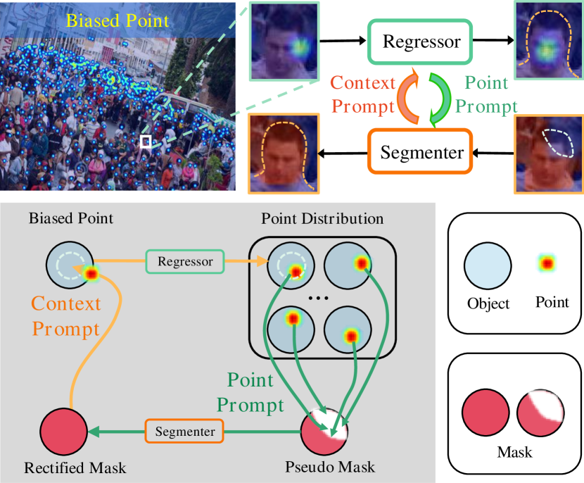
Figure 1: Upper: The biased point annotation impedes accurate model learning. mPrompt leverages context prompt and point prompt to mine spatial context and rectify biased annotation for crowd counting. Lower: Illustration of mutual prompt learning (mPrompt), which completes pseudo segmentation mask by using point prompt learning. Meanwhile, it leverages the rectified masks as spatial context information to refine biased point annotations in a way of context prompt learning. (Best viewed in color)

Unfortunately, point annotations exhibit considerable variances, termed label variance, which impedes the accurate learning of models. As shown in Fig. 1, label variance is an inherent issue, where the annotated point are coarsely placed within head regions rather than at precise center positions. To mitigate the label variance, loss relaxation approaches [41, 54, 56] modified the strict pixel-wise loss constraint via constructing probability density functions. Segmentation-based approaches [42, 67, 49] suppressed background noises by introducing an auxiliary branch to regressor networks [42].

Unfortunately, loss relaxation methods comprise point position variance, which could introduce background noises to the regressor. Segmentation-based methods manage to alleviate label variance using spatial context, but are challenged by the inaccurate context information. To obtain accurate context information while alleviating background noises in a systematic framework remains to be elaborated.

In this study, the pivotal question we seek to address is: How to obtain precise spatial context information to alleviate the impact of label variance for crowd counting? We propose a simple-yet-effective mutual prompt learning framework, Fig. 1, which leverages a regressor and a segmenter as guidance for each other. This framework comprises a head segmenter, a density map regressor, and a mutual learning module. Specifically, mPrompt leverages the point annotation to tune a segmenter and predict pseudo head masks in a way of point prompt learning. As illustration in Fig. 1, the point prompt provides statistical distribution (random and uncertain locations) of points to refine the object mask. The objective of the segmenter is to isolate head regions, so as to learn comprehensive and accurate pseudo segmentation masks. Such pseudo segmentation masks are treated as spatial context to rectify biased point annotations in a way of context prompt learning. This mutual prompt process fosters information gain between the segmenter and the density map regressor, driving them to enhance each other and ultimately reach an optimal state.

The contributions of this study are summarized as follows:

• We propose a mutual prompt learning (mPrompt) framework, which incorporates a segmenter and a regressor and maximizes their complementary for crowd counting. To our best knowledge, this is the first attempt to unify learning accurate context information and alleviating background noises using mutual prompt.

• We design feasible point prompt by unifying the predicted density map with the ground-truth one, and plausible mask prompt by unifying/intersecting the predicted density map with a segmentation mask.

• Experiments conducted on the popular crowd-counting datasets, including ShanghaiTechA/B [66], UCF-QNRF [59] and NWPU [17] demonstrate mPrompt’s effectiveness when addressing label variance. Particularly, mPrompt achieves new state-of-the-art performances on multiple benchmark datasets.

2 Related Work

Density Regression Method. Nowadays, density map regression [28] is widely used in crowd counting [66, 3, 29, 7, 35, 34, 64, 4, 53, 55, 52, 57] due to its simple and effective learning strategies. Nevertheless, many density regression approaches neglected scale variation of heads, and thereby is challenged by the inconsistency between density maps and features caused by labeling variance.

To tackle scale variance, multi-scale feature fusion layers [19, 53, 20], attention mechanisms [35, 64, 21, 32, 12], perspective information [48, 61, 63, 62], and dilated networks [4, 61] were proposed.

To mitigate the side effect of inaccurate point annotations, distribution matching [56, 31], generalized localization loss [55], and density normalized precision [52] are proposed to minimize the discrepancy between the predicted maps and point annotations. For so many approaches proposed, however, density regression remains challenged by the label variance issue, which is expected to be tackled by introducing segmentation-based context information.

Segmentation-based Method. In early years, Chan et al. [8] and Ryan et al. [47] proposed to segment foreground objects to distinct clusters, and regress the features of each cluster to determine the overall object counts. Recent studies [67, 49, 42] began to incorporate image segmentation as an auxiliary task to leverage spatial context information while mitigating the effects of false regression. These methods typically utilized the coarse “ground-truth” segmentation maps, which are simply derived from the noisy point annotation maps. As a result, they lack robust and precise spatial information, and are prone to label variability. In contrast, this study smoothly acquires precise spatial information about head positions, reducing label variance through the deployment of mutual prompt learning. The significant advantage of our approach upon conventional segmentation-based approaches lies in that it can fully explore the statistical distribution (random and uncertain locations) of points to refine the object mask in a way of point prompt learning.

Prompt Learning. In the era of large language models [11, 6], prompt learning has been shown to be a powerful tool for solving various natural language processing (NLP) tasks [36, 45, 6]. various prompt learning strategies including prompt engineering [40, 6], prompt assembling [22], and prompt tuning [44], are respectively proposed. Inspired by the success of prompt learning in NLP, vision prompt learning approaches [18, 5] are proposed. The challenge lies in how to design plausible prompts which can guide and enhance the learning of models on specific tasks.

In this study, we take a further step to mutual prompt learning, with the aim to enhance both the regression and segmentation models in a unified framework. While the term “prompt” typically refers to “guidance/hint” embedding into the pretrained large model in the forward process, our work extends its application to the realm of backward gradient propagation (via point and context prompt in this paper). We also extend our method by integrating pre-trained large-scale models, capitalizing on their extensive knowledge base. This integration enables our model to achieve robust performance while maintaining parameter efficiency during training.

\begin{overpic}[scale={0.9}]{figs/structure_last.pdf} \par\end{overpic}

Figure 2: mPrompt consists of four components: a shared backbone for feature extraction, a regressor for density map ($\hat{y}$) prediction, a segmenter for head region ($\hat{m}$) estimation, and a mutual prompt learning module.

3 The Proposed Approach

The proposed approach integrates a regressor and a segmenter for density map and segmentation mask prediction. In what follows, we first unify the segmenter with a regressor to construct a two-branch network. We then introduce mutual prompt learning to the network, which encompasses point prompts given by the regressor and context prompts provided by the segmenter.

3.1 Unifying Segmenter with Regressor

Network Architecture. As shown in Fig. 2(upper), mPrompt consists of a shared CNN backbone, a density regressor $\mathcal{R}$ and a head segmenter $\mathcal{S}$, which are trained in an end-to-end fashion. The shared backbone is derived from a HRNet by truncating layers from stage4 [58]. To seamlessly unify the segmenter with the regressor, a self-attention module applied to them to enhance features of the regressor, Fig. 2. Denoting $\mathcal{S}(x)$ and $\mathcal{R}(x)$ as the features of the regressor and the segmenter for an input image ${x}$, the self-attention operation is applied on $\mathcal{S}(x)$ and $\mathcal{R}(x)$ as $Sigmoid\big{(}\mathcal{S}(x)\big{)}\bigotimes\mathcal{R}(x)$, where $\bigotimes$ is the element-wise multiplication. With feature self-attention, the regressor preliminarily incorporates the context information provided by the segmenter.

\begin{overpic}[scale={0.22},tics=2]{figs/offline_online.pdf} \end{overpic}

Figure 3: Illustration of the generation of prompt information for the segmenter. White boxes highlight key regions for better clarity. The red-shaded areas represent the head segmentation mask, demonstrating the pseudo mask’s inaccuracy when compared to the more precise updated target mask. With offline prompt, the prompted segmenter tends to predicted more complete head regions but unfortunately introduces background noises. With online prompt, background noises are reduced. (Best viewed in color with zoom)

Figure 4: Illustration of $K$-NN algorithm, which removes background noises from the target segmentation mask.

The regressor predicts the density map $\boldsymbol{\hat{y}}$ for the input image $\boldsymbol{x}$, and the segmenter predicts the head mask $\boldsymbol{\hat{m}}$. The regressor and segmenter are designed using an identical architecture, comprising Conv-BN-ReLU blocks. Specifically, three Conv-BN-ReLU blocks are adopted to decrease the feature channel size progressively from $128$ to $64$, and eventually down to $32$ followed by a self-attention operation. A convolution layer of kernel size $1$ followed by ReLU/Sigmoid layer squeezes the features to density/segmentation maps.

Segmenter Learning. Each point annotation is expanded to a density map ($\boldsymbol{y}$) and a target mask ($\boldsymbol{m}$), which however are noisy and inaccurate. Fortunately, existing datasets, such as NWPU [59], provide point and box annotations, which can be expanded to pseudo masks for segmenter training. A point pseudo mask is derived by applying dilation to the point density map, which are converted to a segmentation mask after binarization. Following [67, 49, 42], we train the segmenter using the cross-entropy loss function $\mathcal{L}_{s}$ defined on point pseudo masks.

As elucidated by experiments, using point-based pseudo masks to train a segmenter exhibits a challenge in assimilating spatial information. This limitation primarily stems from the fact that the learning targets for both the segmenter and regressor are manually created from dot annotations, which intrinsically do not convey any spatial information. To develop an advanced segmenter, we further leverage the box annotations provided by the NWPU dataset [59]. A box pseudo mask is produced by attributing values of $1$ to locations within the heads and $0$ to the background. Accordingly, the overall loss for the regressor and segmenter is defined as $\mathcal{L}=\mathcal{L}_{den}+\lambda_{s}\mathcal{L}_{seg}$ where $\lambda_{s}$ is a parameter to balance the two losses .

3.2 Segmenter Learning with Point Prompt

As shown in Fig. 2, point prompt defines a procedure to refine the target mask $\boldsymbol{m}$ using the pseudo mask ${m}_{p}$, the ground-truth density map $\boldsymbol{y}$ and the predicted density map $\boldsymbol{\hat{y}}$. In specific, we utilize the pseudo mask $\boldsymbol{m}_{p}$ (offline obtained via a segmenter pretrained on NWPU box annotations) and ground-truth density map ($\boldsymbol{y}$) for offline prompt, and the density map $\boldsymbol{\hat{y}}$ for online prompt, which guarantees the renewal of the segmentation map via the prompt from the regressor. When training the segmenter, the binary cross entropy loss is applied.

Offline Prompt. This is performed by unifying the segmentation pseudo mask $\boldsymbol{m}_{p}$ with the binarized ground-truth density map $\boldsymbol{y}$, as

$$\boldsymbol{m}=\boldsymbol{m}_{p}\cup\mathbf{B}({\boldsymbol{y}}),$$ (1)

where $\cup$ denotes the union operation performing pixel-wise OR operation between two matrices. $\mathbf{B}(\cdot)$ defines a binarization function: the density map is binarized with a $0$ threshold to form a mask. Supervised by training targets $\boldsymbol{m}$ from all the training images, the segmenter tends to absorb the distribution (random and uncertain locations) of points. After prompt learning, the prompted segmenter tends to predict more complete head regions (the top row of Fig. 3) where the initialized segmenter fails to predict.

Online Prompt. With the offline prompt, the accuracy of the predicted density map can be improved after $\kappa$ epochs of training, so that it can be used to improve the target segmentation mask. Following the initial $\kappa$ training epochs, $\hat{y}$ should possess credibility and aid in introducing reliable distributions (Gaussian blobs randomly situated around the point annotations) of head regions. As a result, integrating $\hat{y}$ into point prompt learning further assists in predicting the comprehensive head regions. Meanwhile, the union operation defined in offline/online prompt inevitably introduce background noises from the density map to the target mask. To solve, we further leverage a $K$-NN algorithm to filter out background noises (the bottom row of Fig. 3) at the end of online prompt, which defined as interaction operation. Online prompt defines the following union and intersection operations, as

$$\boldsymbol{m}\leftarrow(\boldsymbol{m}\boldsymbol{\cup}(\mathbf{B}({\boldsymbol{\hat{y}}}))\boldsymbol{\cap}\boldsymbol{m}_{K},$$ (2)

where $m_{K}$ is a context mask defined by a spatial $K$-NN algorithm applied on the point annotations Fig. 4. In specific, for a point annotation, the spatial $K$-NN algorithm finds its $K$ nearest point annotations. The minimum circle area covering the $K$ nearest point annotations is defined as the context mask $m_{K}$.

3.3 Regressor Learning via Context Prompt

With point prompt, the segmenter absorbs distribution of the annotated points so that it produces more accurate mask predictions. Such mask predictions serve as a spatial information to improve the regressor in turn, which is termed as context prompt. In specific, the context prompt is defined as a constraint, which encourages the predicted density map $\boldsymbol{\hat{y}}$ falling the target mask $\boldsymbol{m}$. This is implemented by introducing a context prompt loss to the framework, as

$$\boldsymbol{\mathcal{L}}_{con}(\boldsymbol{\hat{y}},\boldsymbol{\hat{m}})=-\frac{\Sigma{\big{(}\mathbf{B}({\boldsymbol{\hat{y}}})}\cap\mathbf{B}({\boldsymbol{\hat{m}}})\big{)}}{\Sigma{\mathbf{B}({\boldsymbol{\hat{y}}})}},$$ (3)

where $\Sigma$ accumulates the values of all pixels. To minimize the context prompt loss, intersection term in Eq. 3 must be large, which implies the prediction $\boldsymbol{\hat{y}}$ of the regressor falling in the predicted mask area ($\boldsymbol{\hat{m}}$) of the segmenter. In other words, the segmenter serves as the context prompt of the regressor. When training the regressor, the conventional MSE constrain is defined as the density map construction loss.

3.4 Mutual Prompt Learning

Given the point prompt defined by Eq. 1 and Eq. 2, and the context prompt defined by Eq. 3, the mutual prompt learning is performed in an end-to-end fashion by optimizing the following loss function,

$$\boldsymbol{\mathcal{L}}=\lambda_{d}\mathcal{L}_{den}(\boldsymbol{\hat{y}},\boldsymbol{y})+\lambda_{s}\mathcal{L}_{seg}(\boldsymbol{\hat{m}},\boldsymbol{m})+\lambda_{c}\mathcal{L}_{con}(\boldsymbol{\hat{y}},\boldsymbol{\hat{m}}),$$ (4)

where $\lambda_{d}$, $\lambda_{s}$ and $\lambda_{c}$ are experimentally defined regularization factors.

In summary, our mPrompt comprises three components: (1) With point prompt learning, the segmenter absorbs statistical distribution (random and uncertain locations) of points to predict more accurate target masks. (2) With context prompt learning, the predicted density map is constrained to fall into the target mask regions, which in turn improve the density regression. (3) Unifying point prompt learning with context prompt learning in a framework with shared backbone and training the network parameters in an end-to-end fashion create mutual prompt learning.

3.5 Extension to Foundation Model

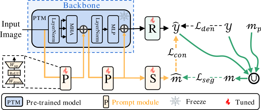
Figure 5: mPrompt with learnable prompt modules based on pre-trained model.

Our mPrompt approach can be further applied to foundation model adaptation. This involves expanding the context prompt into a feature insertion strategy, which enhances the utilization of the extensive knowledge embedded in pre-trained large models, as demonstrated in Fig. 5. In this process, the context prompt is modulated by learnable prompt modules. Such prompt modules are implemented using adapter mechanism [16]. Our primary goal is to integrate comprehensive context information into foundational models, specifically for crowd counting. This aims to make effective use of the representational knowledge in pre-trained large models by only fine-tuning a small number of parameters.

During the inference phase, the learnable prompt modules, along with the backbone and regressor, are retained, while the segmenter branch is discarded. These prompt modules function as context prompts, facilitating the insertion of features into the backbone.

3.6 Interpretive Analysis

The proposed approach is justified from the perspective of mutual information [1]. mPrompt can be generally interpreted as a procedure to maximize the mutual information $\mathcal{I}$ of a regressor ($f^{r}$) and a segmenter ($f^{s}$). The point prompt is interpreted as

$$\mathbf{H}(f^{s},f^{r})=\mathbf{H}(f^{s}|f^{r})+\mathbf{H}(f^{r})$$ (5)

where $\mathbf{H}(\cdot)$ is information entropy, the $\mathbf{H}(f^{s}|f^{r})$ is conditional and the $\mathbf{H}(f^{s},f^{r})$ is joint entropy. Denote the parameters of the model as $\theta$. To minimize $\boldsymbol{\mathcal{L}}_{con}(\boldsymbol{\hat{y}},\boldsymbol{\hat{m}})$ is equivalent to maximize $\log\frac{\Sigma{\big{(}\mathbf{B}({\boldsymbol{\hat{y}}})}\cap\mathbf{B}({\boldsymbol{\hat{m}}})\big{)}}{\Sigma{\mathbf{B}({\boldsymbol{\hat{y}}})}}$. Then the context prompt is interpreted as

$$\begin{split}\arg\max_{\theta}&\ \mathcal{I}_{\theta}(f^{r};f^{s})=\log\frac{p(f^{r}|f^{s})}{p(f^{r})},\end{split}$$ (6)

which maximizes the mutual information between the regressor $f^{r}$ and the segmenter $f^{s}$.

Method	Venue	SHA		SHB		QNRF		NWPU(V)		NWPU(T)
		MAE	RMSE	MAE	RMSE	MAE	RMSE	MAE	RMSE	MAE	RMSE
GLoss [55]	CVPR’21	61.3	95.4	7.3	11.7	84.3	147.5	-	-	79.3	346.1
UEPNet [57]	ICCV’21	54.6	91.2	6.4	10.9	81.1	131.7	-	-	-	-
P2PNet [52]	ICCV’21	52.8	85.1	6.3	9.9	85.3	154.5	77.4	362.0	83.3	553.9
DKPNet [9]	ICCV’21	55.6	91.0	6.6	10.9	81.4	147.2	61.8	438.7	74.5	327.4
SASNeT [53]	AAAI’21	53.6	88.4	6.4	9.9	85.2	147.3	-	-	-	-
ChfL [50]	CVPR’22	57.5	94.3	6.9	11.0	80.3	137.6	76.8	343.0	-	-
GauNet [10]	CVPR’22	54.8	89.1	6.2	9.9	81.6	153.7	-	-	-	-
MAN [32]	CVPR’22	56.8	90.3	-	-	77.3	131.5	76.5	323.0	-	-
S-DCNet (dcreg) [60]	ECCV’22	59.8	100.0	6.8	11.5	-	-	-	-	-	-
CLTR [30]	ECCV’22	56.9	95.2	6.5	10.6	85.8	141.3	61.9	246.3	74.3	333.8
DDC [46]	CVPR’23	52.9	85.6	6.1	9.6	65.8	126.5	-	-	-	-
PET [33]	ICCV’23	49.3	78.8	6.2	9.7	79.5	144.3	58.5	238.0	74.4	328.5
STEERER [14]	ICCV’23	54.5	86.9	5.8	8.5	74.3	128.3	54.3	238.3	63.7	309.8
mPrompt‡ (ours)	-	52.5	88.9	5.8	9.6	72.2	133.1	50.2	219.0	62.1	293.5
mPrompt‡∗ (ours)	-	53.2	85.4	6.3	9.8	76.1	133.4	58.8	240.2	66.3	308.4

Table 1: Performance comparisons. mPrompt_‡^∗ indicates that we extend the mPrompt to the pre-trained model (SAM-base). The best results are shown in bold, and the second-best results are underlined.

4 Experiment

Dataset: Experiments are carried out on four public crowd counting datasets including ShanghaiTechA/B [66], UCF-QNRF [17], and NWPU [59]. ShanghaiTech includes PartA (SHA) and PartB (SHB), totaling $1,198$ images with $330,165$ annotated heads. SHA comprises $300$ training images and $182$ testing images with crowd sizes from $33$ to $3,139$. SHB includes $400$ training images and $316$ testing images with crowd sizes ranging from $9$ to $578$. The images are captured from Shanghai street views. UCF-QNRF (QNRF) encompasses $1,535$ high-resolution images, $1.25$ million annotated heads with extreme crowd congestion, small head scales, and diverse perspectives. It is divided into $1,201$ training and $334$ testing images. NWPU dataset comprises $5,109$ images, with $2,133,375$ annotated heads and head box annotations. The images are split to a training set of $3,109$ images, an evaluation set of $500$ images, and a testing set of $1,500$ images. NWPU(V) and NWPU(T) denote the validation and testing sets, respectively.

Evaluation Metric: Mean Absolute Error (MAE) and Root Mean Squared Error (RMSE) [29, 37] are used. They are defined as $M\!A\!E=\frac{1}{N}\sum^{N}_{i=1}|\hat{C}_{i}-C_{i}|$ and $R\!M\!S\!E=\sqrt{\frac{1}{N}\sum^{N}_{i=1}|\hat{C}_{i}-C_{i}|^{2}}$, where $N$ is the number of test images. $\hat{C}_{i}$ and ${C}_{i}$ respectively denote the estimated and ground truth counts of image $x_{i}$.

Implementation Details: We resize images to a maximum length of $2,048$ pixels and a minimum of $416$ pixels, keeping the aspect ratio unchanged. Data augmentation includes random horizontal flipping, color jittering, and random cropping with a $400\times 400$ pixel patch size. Ground-truth density maps are generated using a $15\times 15$ Gaussian kernel. The network is trained using Adam [24] optimizer with learning rate of $1e^{-4}$. The batch size is $16$ and training on NWPU dataset takes about $25$ hours on four Nvidia V100 GPUs. Key parameters include $K=3$, $\lambda_{d}=1$, $\lambda_{s}=0.5$, $\lambda_{c}=0.5$ and $\kappa=50$. The network is constructed with the backbone HRNet-W40-C [58] pretrained on ImageNet [27] and random initialization of the remaining parameters. When adopting mPrompt for foundation models, we utilize SAM-base [26], chosen for its robust segmentation performance. We train both networks for 700 epochs.

In Table 1, the performance of mPrompt_‡ is compared with state-of-the-art methods across four major datasets. mPrompt_‡ consistently achieves impressive results in terms of MAE on all four datasets. mPrompt_‡ consistently ranks within the top-2 for MAE performance across the datasets, highlighting the superior effectiveness of our model.

4.1 Visualization Analysis

Fig. 6 visualizes the predicted density maps and the attention map from a test image. mPrompt_‡ generates more precise density maps compared with the baseline (mPrompt_rsg), at both dense and sparse regions. Particularly, after the context prompt learning, mPrompt_‡ indeed isolates the accurate head regions as the regressor absorbs the context information from the segmenter.

Fig. 7 visualizes the segmentation maps predicted by mPrompt_rsg and mPrompt_‡. Specifically, we identify three types of regions when comparing these two segmentation maps. Blue and yellow regions are generated by mPrompt_rsg (baseline) and mPrompt_‡, respectively. Red regions represent the intersection of these two masks. One can see that mPrompt_‡ improves head region segmentation by removing areas where the background is mistaken for a head and adding regions where the head is mistaken for background, compared to the baseline. In order to evaluate the enhancement of the segmenter, we conduct an analysis of the Intersection over Union (IoU) between the head-box regions and the predicted mask on the NWPU dataset. This investigation yields IoU scores of $46.5$ for mPrompt_‡ and $38.7$ for mPrompt_rsg, respectively, thus providing quantitative evidence of the segmenter’s improvement through mPrompt_‡. These validate the effect of point prompt learning, which finally contributes to the superior performance reported in Table 2.

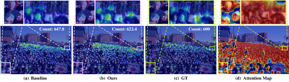
Figure 6: Comparison of the density maps with/without context prompt. (Best viewed in color with zoom)

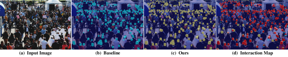
Figure 7: Comparison of segmentation masks with/without point prompt. (Best viewed in color with zoom)

4.2 Ablation Studies

Methods	Regressor	Segmenter	Point Prompt		Context	SHA	SHB	QNRF	NWPU(V)
			Offline	Online	Prompt
mPromptreg	$\checkmark$					59.4	7.8	85.5	65.7
mPromptrsg	$\checkmark$	$\checkmark$				58.4	7.1	83.2	64.3
mPromptp†	$\checkmark$	$\checkmark$	$\checkmark$			54.8	6.2	78.9	59.2
mPromptp‡	$\checkmark$	$\checkmark$	$\checkmark$	$\checkmark$		53.9	5.9	74.8	52.1
mPromptc†	$\checkmark$	$\checkmark$			$\checkmark$	55.3	6.4	79.4	62.0
mPrompt†	$\checkmark$	$\checkmark$	$\checkmark$		$\checkmark$	54.1	6.1	76.7	56.5
mPrompt‡	$\checkmark$	$\checkmark$	$\checkmark$	$\checkmark$	$\checkmark$	52.5	5.8	72.2	50.2

Table 2: Ablation study of mPrompt components about MAE.

Backbones	#Params(M)	GFLOPs	mPromptreg		mPromptrsg		mPrompt†		mPrompt‡
			MAE	RMSE	MAE	RMSE	MAE	RMSE	MAE	RMSE
CNN architecture
VGG19 [51]	12.6	19.3	64.0	112.5	62.6	106.5	61.4	100.9	60.9	106.1
HRNet [58]	33.1	62.1	59.4	96.7	58.4	95.8	54.1	92.8	52.5	88.9
Transformer architecture
Swin [38]	7.4	11.6	63.9	105.5	61.8	100.0	61.1	99.3	59.3	98.8
SAM [25]	7.7	13.5	60.4	98.3	59.5	98.8	55.2	89.5	53.2	85.4

Table 3: Comparison of backbones on the SHA dataset is paired with an analysis of learnable parameters and FLOPs for a standard input size of ($3\times 224\times 224$) when training.

No Mutual Prompt Learning
Method	Seg label		SHA	SHB	QNRF	NU(V)
	point	box
mPtrsg∗	$\checkmark$		58.8	7.5	84.3	66.8
mPtrsg		$\checkmark$	58.4	7.1	83.2	64.3
Mutual Prompt Learning
Method	$\boldsymbol{m_{p}}$		SHA	SHB	QNRF	NU(V)
	mPtrsg∗	mPtrsg
mPt‡∅	$\emptyset$		54.6	6.3	73.9	52.1
mPt‡∗	$\checkmark$		54.3	6.4	73.4	52.7
mPt‡		$\checkmark$	52.5	5.8	72.2	50.2

Table 4: Performance when adopting different pseudo masks. Due to space constraints, we use the abbreviations NU(V) and mPt to respectively refer to NWPU(V) and mPrompt.

No Prompt. The baseline mPrompt_reg consists only a regressor. By introducing the segmenter and employing pseudo mask as supervision, mPrompt_reg develops to mPrompt_rsg. In Table 2, mPrompt_reg harnesses the robust features of HRNet (truncated at stage4), achieving competitive MAE performances of $59.4$, $7.8$, $85.5$, and $65.7$ on SHA, SHB, QNRF, and NWPU(V) datasets, respectively. mPrompt_rsg surpasses mPrompt_reg, highlighting the significance of introducing the segmenter and signifying the effective utilization of spatial head information.

Point Prompt. With offline and online point prompt, mPrompt_rsg promotes to mPrompt_p† and mPrompt_p‡, respectively. mPrompt_p† achieves better performance, reaching MAEs of $54.8$, $6.2$, $78.9$, and $59.2$ on SHA, SHB, QNRF, and NWPU(V) datasets, respectively. mPrompt_p‡ further reduces the MAEs to $53.9$, $5.9$, $74.8$, and $52.1$ on these four datasets.

Context Prompt. In Table 2, when adopting $\mathcal{L}_{con}$ to mPrompt_rsg, our mPrompt_c† delivers a performance gain on these datasets, indicating the necessity of spatial information for regressing implemented in this explicit manner.

Mutual Prompt. In Table 2, both mPrompt${\dagger}$ and mPrompt${\ddagger}$ achieves satisfying performances, and our final variant mPrompt${\ddagger}$ delivers MAEs of $52.5$, $5.8$, $72.2$, and $50.2$ on SHA, SHB, QNRF, and NWPU(V) datasets, respectively. Comparing with mPrompt_reg, a significant performance gain is achieved, reducing MAE by $6.9$, $2.0$, $13.3$, and $15.5$, respectively. These ablation studies validate the efficacy of the components of mPrompt.

Pseudo masks. We use a segmenter pretrained on NWPU box annotations to obtain the offline pseudo mask $\boldsymbol{m}_{p}$. A natural question arises: Can we generate $\boldsymbol{m}_{p}$ using a segmenter pretrained only with the point annotations, or even directly set $\boldsymbol{m}_{p}$ as $\emptyset$? To explore this, we pretrain mPrompt_rsg∗ using only the point annotations of the corresponding dataset to generate the segmentation masks (i.e., point-based pseudo mask). In Table 4, mPrompt_rsg∗ underperforms mPrompt_rsg due to the inaccuracy of the segmentation label. By setting $\boldsymbol{m_{p}}$ to $\emptyset$ and utilizing pseudo masks generated from mPrompt_rsg∗ and mPrompt_rsg in mutual prompt learning, we obtain mPrompt_‡∅, mPrompt_‡∗ and mPrompt_‡, respectively. mPrompt_‡∗ performs similarly to mPrompt_‡∅, as $\boldsymbol{m}_{p}$ indeed introduces no extra spatial information when only utilizing the pseudo masks generated from mPrompt_‡∗. Even with $\boldsymbol{m}_{p}$ set to $\emptyset$, mPrompt_‡∅ still significantly outperforms mPrompt_reg∗, highlighting the effectiveness of mutual prompt learning.

Backbone Architectures. We replace HRNet-W40-C with other commonly-used backbones (VGG19 [51], Swin [38] and SAM [25]). Table 3 reveals that mPrompt_‡ continues to outperform mPrompt_reg, mPrompt_rsg, and mPrompt_†, achieving significant MAE reductions. Furthermore, we have extended the mPrompt to foundational models, such as the SAM [25] and Swin [38]. As shown in Table 3, mPrompt_‡ (SAM based) shows performance marginally below mPrompt_‡, yet with only about $\frac{1}{4}$ the training parameters and $\frac{1}{5}$ the FLOPs of the latter. For crowd counting, given the backbone is static and only the prompt module is learnable, the Swin Transformer, pretrained for classification, underperforms compared to SAM [25]. This mainly attributes to Swin’s representational knowledge is less aligned with crowd counting comparing with SAM.

Robustness to Annotation Variance. To assess the robustness of mutual prompt learning against box annotation variance, we conduct an experiment on NWPU, observing performance changes with varying box annotations. Specifically, we add uniform random noise, ranging from $0$ to $50\%$, of the box height, to the official annotated boxes. Fig. 8 reveals that our mPrompt_‡ is only mildly affected by different noise levels, while mPrompt_rsg and STEERER [14] suffer from severe performance degradation. This demonstrates the robustness of our mPrompt_‡ to annotation variance.

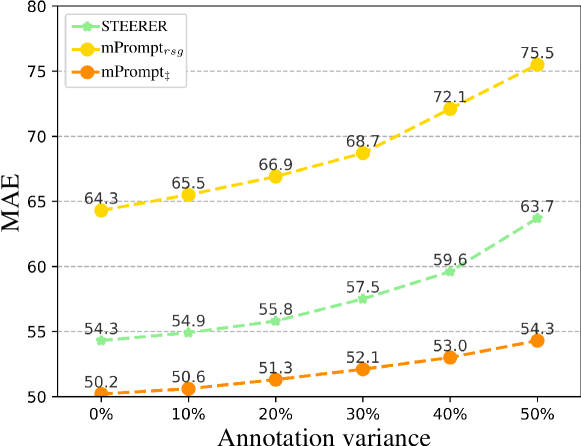
Figure 8: Performance on NWPU when training with different annotation variance.

5 Conclusions

We proposed a mutual prompt learning approach, to enhance context information while mitigating the impact of point annotation variance in crowd counting. mPrompt incorporates a shared backbone, a density map regressor for counting, a head segmenter for foreground and background distinction. The mutual prompt learning strategy maximized the mutual information gain of the segmenter and regressor. Experimental results on four public datasets affirm the efficacy and superiority of our method. While we primarily focus on crowd density maps in this study, mPrompt has potential applications in areas with scarce or noisy labeling information, such as crowd localization, object detection, and visual tracking. We aim to explore these applications in the future work.

Appendix A Details of Training a Segmenter

Training via point Annotation. For methods [67, 49, 42], they adopt point-segmentation map $P$ as the target of the segmenter, as formulated in Equation (7).

$$\mathcal{L}_{poi}=-\sum^{N}_{i=1}\sum^{(H,W)}_{(h=1,w=1)}p(h,w)\log\hat{p}(h,w),$$ (7)

where $N$ is the batch size, $H$ and $W$ are the height and width of image $x_{i}$, respectively. $p(h,w)$ represents the value of position $(h,w)$ in binarized ground-truth density map $P_{i}$, and $\hat{p}(h,w)$ is the corresponding predicted value. To this end, we build the mPrompt_poi under the loss $\mathcal{L}_{poi}$, formulated as

$$\boldsymbol{\mathcal{L}}=\mathcal{L}_{den}+\lambda_{s}\mathcal{L}_{poi},$$ (8)

where $\lambda_{s}$ is a super-parameter to balance the two losses.

As elucidated in scratch, mPrompt_poi exhibits a challenge in assimilating spatial information. This limitation primarily stems from the fact that the targets for both the segmenter and regressor are manually created from dot annotations, which intrinsically do not convey any spatial information.

Training via Box Annotation. To strengthen the segmenter’s ability in integrating spatial information, we pretrain it using head-box annotations of NWPU [59] dataset, and generate pseudo mask ($m_{p}$) of all datastes for mutual prompt learning. Concretely, suppose $B_{i,v}$ is the $v$-th box annotation in the image $x_{i}$ and its annotation is $(x_{l},y_{l},x_{r},y_{r})$ representing upper-left corner and lower-right corner. The head box region $R_{i,v}$ is defined as:

$$\begin{split}&B^{i,v}_{x_{min}}=x_{l},B^{i,v}_{y_{min}}=y_{l},B^{i,v}_{x_{max}}=x_{r},B^{i,v}_{y_{max}}=y_{r}\\ &R^{i}_{v}=\left\{(x,y)|B^{i,v}_{x_{min}}\leq x\leq B^{i,v}_{x_{max}},B^{i,v}_{y_{min}}\leq y\leq B^{i,v}_{y_{max}}\right\}\\ \end{split}$$ (9)

Then the ground-truth box-segmentation map $S_{i}$ for pretraining the head segmenter is defined as

$$S_{i}=\cup^{V_{i}}_{v=1}R^{i}_{v},$$ (10)

where $V_{i}$ denotes the number of boxes in image $x_{i}$ and $\cup$ indicates the union operator. In this case, for $s(h,w)$ which indicates the value of position $(h,w)$ in the $S_{i}$ , we have

$$s(h,w)=\mathbb{I}\left((h,w)\in S_{i}\right).$$ (11)

The function $\mathbb{I}(cond)$ is the indicator function, which is equal to $1$ only if the condition holds, and $0$ otherwise. We utilize $\mathcal{L}_{box}$ to encourage the segmenter to predict a value of $1$ for positions falling within any heads, and a value of $0$ for positions outside them. Formulately, $\mathcal{L}_{box}$ is defined as

$$\mathcal{L}_{box}=-\sum^{N}_{i=1}\sum^{(H,W)}_{(h=1,w=1)}s(h,w)\log\hat{s}(h,w),$$ (12)

where $N$ is the batch size, $H$ and $W$ are the height and width of image $x_{i}$, resp. $s(h,w)$ represents the value of position $(h,w)$ in $S_{i}$, and $\hat{s}(h,w)$ is the corresponding predicted value.

Similar to $\mathcal{L}_{poi}$ and $\mathcal{L}_{box}$, $\mathcal{L}_{seg}$ in manuscript is implemented on density map ($\hat{y}$) and the pseudo mask ($m_{p}$) generated by the pretrained segmenter. Finally, mPrompt is trained with $\mathcal{L}_{seg}$ as follows:

$${\mathcal{L}}=\mathcal{L}_{den}+\lambda_{s}\mathcal{L}_{seg}$$ (13)

where $\lambda_{s}$ balances the two losses.

Appendix B Details of Extension to Foundation Model

The broadly acknowledged foundational model SAM [25] for image segmentation functions at the pixel level, similar to crowd counting tasks based on density map method. Therefore, SAM has been selected as the foundation model for extending our mPrompt approach, aiming at modifying the hidden representations of a frozen pre-trained model.

The position of adapter. The pre-trained SAM’s image encoder, equipped with adapter modules identical to the scaled parallel adapter [15], has supplanted the backbone of our previous architecture. We fixed the parameters of the image encoder, making only a few parameters trainable, including the adapter modules, regressor and segmenter. Specifically, the image encoder is composed of 12 stacked blocks, each containing two types of sublayers: multi-head self-attention (MHA) and a fully connected feed-forward network (FFN).

Adapters are utilized to modify the outputs of MHA and FFN in the transformer blocks. The output from the last adapter module serves as the input for the segmenter. Throughout this process, the adapter modules function as a context prompt (akin to mask prompts in SAM), referred to here as learnable prompt modules.

The performance of training with adapter. To further validate the potential performance enhancement of mPrompt on foundation model, we evaluated its effectiveness on SHA under the same architecture (image encoder + adapter + regressor + segmenter), but with varied training strategies. These strategies include full fine-tuning without mutual prompt learning, adapter training without mutual prompt learning, and learnable prompt modules with mutual prompt learning. As presented in Table 5, it is evident that our method offers significant improvement opportunities when applied to foundational model.

full ft	adapter	mPrompt
54.8	56.2	53.2

Table 5: Performance on SHA about MAE, when adopting different training strategies.

Appendix C Analysis of Convergence Speed via Context Constraint

We have introduced $\mathcal{L}_{con}$ as a mechanism to guide non-zero values of the density map ($\hat{y}$) to fall within mask ($\hat{m}$), a crucial factor for achieving rapid convergence of the regressor. To validate this assertion, we conducted an experiment comparing convergence speed based on the inclusion or exclusion of $\mathcal{L}_{con}$. Figure 9 displays the Mean Absolute Errors (MAEs) and Mean Squared Errors (MSEs) of the initial 100 epochs during the training process on SHA. The green curve represents the model trained without $\mathcal{L}_{con}$ ($\lambda_{con}=0$), while the blue curve signifies the model trained with $\lambda_{con}=1$. Upon examining these results, it becomes clear that both the MAEs and MSEs of the model trained with $\lambda_{con}=1$ are consistently lower than those of the model trained without it. These findings underscore that the incorporation of $\lambda_{con}$ effectively aids in achieving faster convergence of the regressor.

\begin{overpic}[scale={0.28}]{figs/mae_mse_convergence.pdf} \par\put(26.0,1.0){\scalebox{0.9}{Epoch}} \put(76.0,1.0){\scalebox{0.9}{Epoch}} \par\put(39.0,29.5){\scalebox{0.7}{$\lambda_{con}$= 1}} \put(89.0,29.5){\scalebox{0.7}{$\lambda_{con}$= 1}} \par\put(39.0,32.5){\scalebox{0.7}{$\lambda_{con}$= 0}} \put(89.0,32.5){\scalebox{0.7}{$\lambda_{con}$= 0}} \par\end{overpic}

Figure 9: MAEs and MSEs of $\lambda_{con}=0$ and $\lambda_{con}=1$.

Appendix D Hyper-parameters

We investigate hyper-parameters including $K$ in $K$-NN, epoch $\kappa$ to begin online point prompt, and loss weights $\lambda_{d}$, $\lambda_{s}$, $\lambda_{c}$. Grid-search is infeasible due to computational constraints. Initially, we explore $K$ while fixing other settings at $\kappa=0$, $\lambda_{d}=\lambda_{s}=\lambda_{c}=1$. Fig. 10 reveals $K=3$ as optimal, yielding the lowest MAE of $55.0$. Using $K=3$, we find $\kappa=50$ reduces MAE to $53.3$. Two conclusions can be drawn: 1) An appropriate $K$ can reduce MAE by approximately a gap of $1$. For very large $K$ values ($e.g.$, $K=5$), the performance is similar to $K=0$. This occurs because a large $K$ means $m_{K}$ covers nearly the entire image, rendering $m_{K}$ almost ineffective. 2) $\kappa=50$ delivers the best MAE, indicating the learning of regressor is fast due to the deployment of $\mathcal{L}_{con}$.

In Table 10, our approach, even when applied with a basic hyper-parameter search, successfully reduces MAE to $52.5$. This is achieved with the settings $\lambda_{d}=1$, $\lambda_{s}=0.5$, and $\lambda_{c}=0.5$. We further have the following two conclusions: 1) Employing only $\mathcal{\lambda}_{d}$, the network still reduces MAE to MAE $58.4$, a marginally performance gain compared to mPrompt_reg. This affirms the rationality of incorporating the attention as implicit spatial context from segmenter to regressor. Additionally, when $\mathcal{\lambda}_{s}$ and $\mathcal{\lambda}_{c}$ are incorporated into the network learning process, we observe further performance gain, underlining the effect of these elements. 2) Upon examining the last three row in Table 10, we confirm that appropriate selection of loss weights can further help enhance performance.

\begin{overpic}[scale={0.35}]{figs/mae.pdf} \put(27.0,0.0){\scalebox{0.8}{$K$}} \put(74.0,0.0){\scalebox{0.9}{$\kappa$}} \end{overpic}

Figure 10: Evaluation of $K$ and $\kappa$ on SHA.

$\lambda_{d}$	$\lambda_{s}$	$\lambda_{c}$	MAE
1	0	0	58.4
1	1	0	55.9
1	1	1	53.3
1	0.5	1	53.7
1	1	0.5	53.5
1	0.5	0.5	52.5

Table 6: Regularization factors.

Appendix E Visualization of mPrompt on Tackling Point Annotation Variance in Highly Congested Scenarios

In this section, we delve deeper into the validation of mPrompt’s efficiency in addressing point annotation variance in highly crowded scenarios. Figure 11 exhibits the respective density maps as predicted by mPrompt_‡ and mPrompt_reg (named “baseline” in the image). In the presented graphic, we have highlighted certain regions using color-coded boxes for ease of understanding. The areas shaded in blue represent the background regions, wherein mPrompt_reg exhibits high activations, contrasting with mPrompt_‡, which does not. In the regions designated by red boxes, we demonstrate the head areas where mPrompt_reg displays inaccurate density blobs, whereas mPrompt_‡ successfully predicts accurate blobs. The white boxes highlight the head areas that mPrompt_reg failed to identify correctly, while, conversely, mPrompt_‡ delivers correct activations. Lastly, the yellow boxes underscore the head regions where mPrompt_reg exhibits activations displaced from the center of the corresponding boxes. In contrast, mPrompt_‡ generates density blobs precisely at the center of the heads. In summary, for all these four identified situations, mPrompt_‡ consistently outperforms mPrompt_reg in accurately predicting head density blobs.

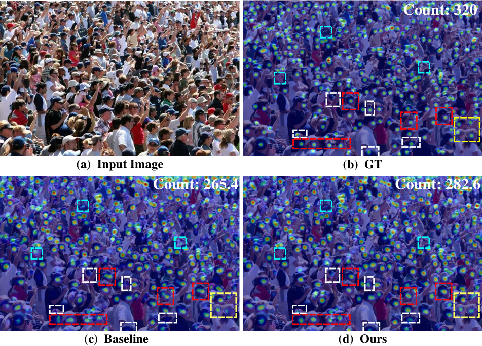
Figure 11: Visualization of density maps. (Best viewed in color)

Appendix F Visualization of mPrompt on Predicting Density Maps

In the main manuscript, we have previously illustrated a selection of examples from the ShanghaiTech Part A (SHA) dataset. We now expand on this by presenting additional visual results derived from ShanghaiTech Part A (SHA), ShanghaiTech Part B (SHB), UCF-QNRF (QNRF), and NWPU Crowd (NWPU) datasets, corresponding to their respective test samples. As can be observed in Figures 12 13 14 15, mPrompt_‡ consistently outperforms mPrompt_reg in generating superior density maps. This superiority is apparent across various regions, whether dense or sparse, in each of the SHA, SHB, QNRF, and NWPU datasets. Thus, mPrompt_‡ demonstrates marked improvement in performance across different types of crowd scenes.

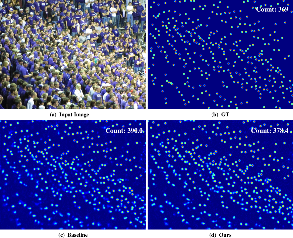
Figure 12: Visualization of predicted density maps from SHA.

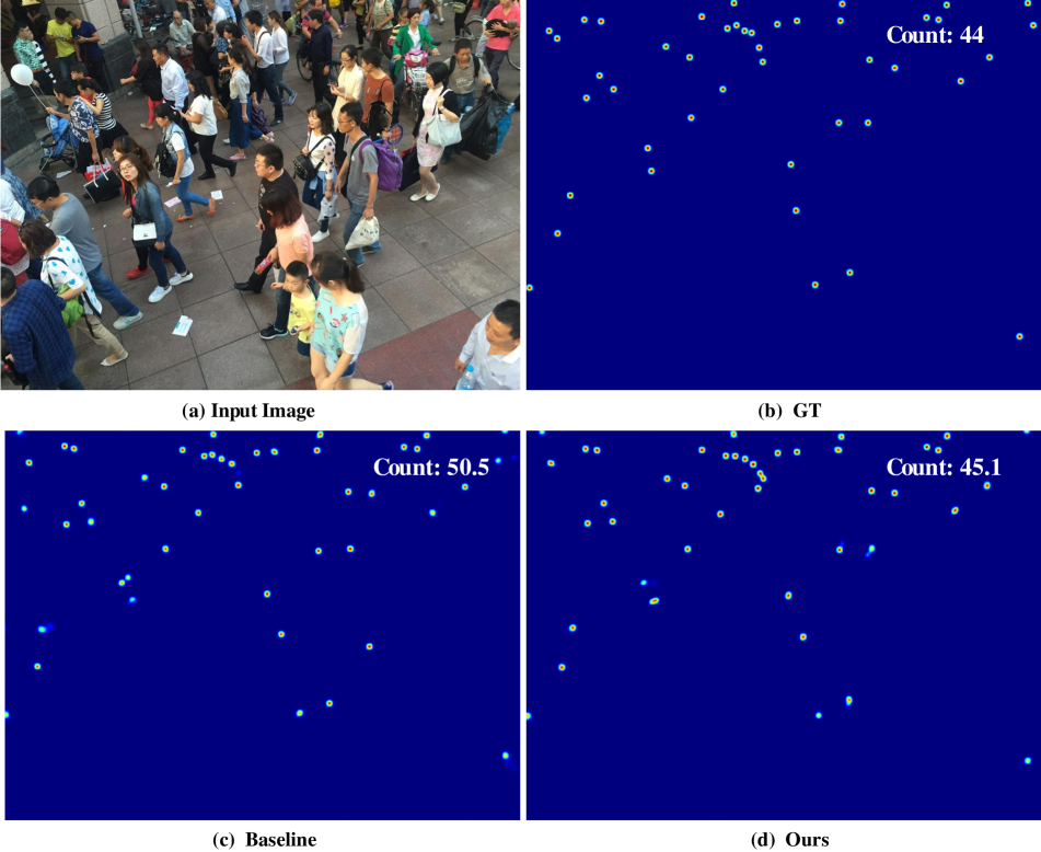
Figure 13: Visualization of predicted density maps from SHB.

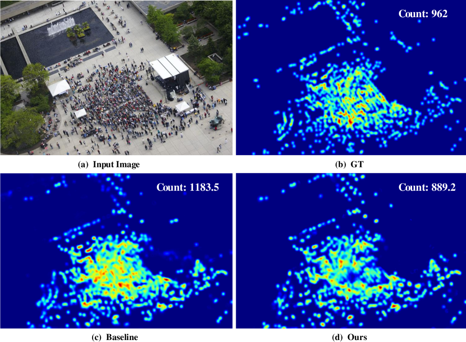
Figure 14: Visualization of predicted density maps from QNRF.

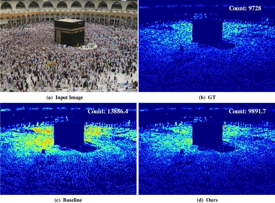
Figure 15: Visualization of predicted density maps from NWPU.

References

- Ahn et al. [2019] Sungsoo Ahn, Shell Xu Hu, Andreas Damianou, Neil D Lawrence, and Zhenwen Dai. Variational information distillation for knowledge transfer. In CVPR, 2019.
- Aich and Stavness [2017] Shubhra Aich and Ian Stavness. Leaf counting with deep convolutional and deconvolutional networks. In ICCV, 2017.
- Babu Sam et al. [2017] Deepak Babu Sam, Shiv Surya, and R Venkatesh Babu. Switching convolutional neural network for crowd counting. In CVPR, 2017.
- Bai et al. [2020] Shuai Bai, Zhiqun He, Yu Qiao, Hanzhe Hu, Wei Wu, and Junjie Yan. Adaptive dilated network with self-correction supervision for counting. In CVPR, 2020.
- Bar et al. [2022] Amir Bar, Yossi Gandelsman, Trevor Darrell, Amir Globerson, and Alexei Efros. Visual prompting via image inpainting. In NIPS, 2022.
- Brown et al. [2020] Tom Brown, Benjamin Mann, Nick Ryder, Melanie Subbiah, Jared D Kaplan, Prafulla Dhariwal, Arvind Neelakantan, Pranav Shyam, Girish Sastry, Amanda Askell, et al. Language models are few-shot learners. In NIPS, 2020.
- Cao et al. [2018] Xinkun Cao, Zhipeng Wang, Yanyun Zhao, and Fei Su. Scale aggregation network for accurate and efficient crowd counting. In ECCV, 2018.
- Chan et al. [2008] Antoni B Chan, Zhang-Sheng John Liang, and Nuno Vasconcelos. Privacy preserving crowd monitoring: Counting people without people models or tracking. In CVPR, 2008.
- Chen et al. [2021] Binghui Chen, Zhaoyi Yan, Ke Li, Pengyu Li, Biao Wang, Wangmeng Zuo, and Lei Zhang. Variational attention: Propagating domain-specific knowledge for multi-domain learning in crowd counting. In ICCV, 2021.
- Cheng et al. [2022] Zhi-Qi Cheng, Qi Dai, Hong Li, Jingkuan Song, Xiao Wu, and Alexander G Hauptmann. Rethinking spatial invariance of convolutional networks for object counting. In CVPR, 2022.
- Devlin et al. [2019] Jacob Devlin, Ming-Wei Chang, Kenton Lee, and Kristina Toutanova. Bert: Pre-training of deep bidirectional transformers for language understanding. In NAACL-HLT, 2019.
- Dong et al. [2022] Li Dong, Haijun Zhang, Jianghong Ma, Xiaofei Xu, Yimin Yang, and QM Jonathan Wu. Clrnet: A cross locality relation network for crowd counting in videos. TNNLS, 2022.
- Guerrero-Gómez-Olmedo et al. [2015] Ricardo Guerrero-Gómez-Olmedo, Beatriz Torre-Jiménez, Roberto López-Sastre, Saturnino Maldonado-Bascón, and Daniel Onoro-Rubio. Extremely overlapping vehicle counting. In IbPRIA, 2015.
- Han et al. [2023] Tao Han, Lei Bai, Lingbo Liu, and Wanli Ouyang. Steerer: Resolving scale variations for counting and localization via selective inheritance learning. In ICCV, 2023.
- He et al. [2021] Junxian He, Chunting Zhou, Xuezhe Ma, Taylor Berg-Kirkpatrick, and Graham Neubig. Towards a unified view of parameter-efficient transfer learning. arXiv preprint arXiv:2110.04366, 2021.
- Houlsby et al. [2019] Neil Houlsby, Andrei Giurgiu, Stanislaw Jastrzebski, Bruna Morrone, Quentin de Laroussilhe, Andrea Gesmundo, Mona Attariyan, and Sylvain Gelly. Parameter-efficient transfer learning for NLP. In ICML, 2019.
- Idrees et al. [2018] Haroon Idrees, Muhmmad Tayyab, Kishan Athrey, Dong Zhang, Somaya Al-Maadeed, Nasir Rajpoot, and Mubarak Shah. Composition loss for counting, density map estimation and localization in dense crowds. In ECCV, 2018.
- Jia et al. [2022] Menglin Jia, Luming Tang, Bor-Chun Chen, Claire Cardie, Serge Belongie, Bharath Hariharan, and Ser-Nam Lim. Visual prompt tuning. In ECCV, 2022.
- Jiang et al. [2019a] Xiaolong Jiang, Zehao Xiao, Baochang Zhang, Xiantong Zhen, Xianbin Cao, David Doermann, and Ling Shao. Crowd counting and density estimation by trellis encoder-decoder networks. In CVPR, 2019a.
- Jiang et al. [2019b] Xiaoheng Jiang, Li Zhang, Pei Lv, Yibo Guo, Ruijie Zhu, Yafei Li, Yanwei Pang, Xi Li, Bing Zhou, and Mingliang Xu. Learning multi-level density maps for crowd counting. TNNLS, 2019b.
- Jiang et al. [2020a] Xiaoheng Jiang, Li Zhang, Mingliang Xu, Tianzhu Zhang, Pei Lv, Bing Zhou, Xin Yang, and Yanwei Pang. Attention scaling for crowd counting. In CVPR, 2020a.
- Jiang et al. [2020b] Zhengbao Jiang, Frank F Xu, Jun Araki, and Graham Neubig. How can we know what language models know? TACL, 2020b.
- Kang et al. [2018] Di Kang, Zheng Ma, and Antoni B Chan. Beyond counting: Comparisons of density maps for crowd analysis tasks—counting, detection, and tracking. TCSVT, 2018.
- Kingma and Ba [2014] Diederik P Kingma and Jimmy Ba. Adam: A method for stochastic optimization. arXiv preprint, 2014.
- Kirillov et al. [2023a] Alexander Kirillov, Eric Mintun, Nikhila Ravi, Hanzi Mao, Chloe Rolland, Laura Gustafson, Tete Xiao, Spencer Whitehead, Alexander C. Berg, Wan-Yen Lo, Piotr Dollár, and Ross Girshick. Segment anything. arXiv:2304.02643, 2023a.
- Kirillov et al. [2023b] Alexander Kirillov, Eric Mintun, Nikhila Ravi, Hanzi Mao, Chloe Rolland, Laura Gustafson, Tete Xiao, Spencer Whitehead, Alexander C Berg, Wan-Yen Lo, et al. Segment anything. arXiv preprint arXiv:2304.02643, 2023b.
- Krizhevsky et al. [2012] Alex Krizhevsky, Ilya Sutskever, and Geoffrey E Hinton. Imagenet classification with deep convolutional neural networks. Advances in neural information processing systems, 25, 2012.
- Lempitsky and Zisserman [2010] Victor Lempitsky and Andrew Zisserman. Learning to count objects in images. In NIPS, 2010.
- Li et al. [2018] Yuhong Li, Xiaofan Zhang, and Deming Chen. Csrnet: Dilated convolutional neural networks for understanding the highly congested scenes. In CVPR, 2018.
- Liang et al. [2022] Dingkang Liang, Wei Xu, and Xiang Bai. An end-to-end transformer model for crowd localization. In ECCV, 2022.
- Lin et al. [2021] Hui Lin, Xiaopeng Hong, Zhiheng Ma, Xing Wei, Yunfeng Qiu, Yaowei Wang, and Yihong Gong. Direct measure matching for crowd counting. IJCAI, 2021.
- Lin et al. [2022] Hui Lin, Zhiheng Ma, Rongrong Ji, Yaowei Wang, and Xiaopeng Hong. Boosting crowd counting via multifaceted attention. In CVPR, 2022.
- Liu et al. [2023] Chengxin Liu, Hao Lu, Zhiguo Cao, and Tongliang Liu. Point-query quadtree for crowd counting, localization, and more. In ICCV, 2023.
- Liu et al. [2019a] Lingbo Liu, Zhilin Qiu, Guanbin Li, Shufan Liu, Wanli Ouyang, and Liang Lin. Crowd counting with deep structured scale integration network. In ICCV, 2019a.
- Liu et al. [2019b] Ning Liu, Yongchao Long, Changqing Zou, Qun Niu, Li Pan, and Hefeng Wu. Adcrowdnet: An attention-injective deformable convolutional network for crowd understanding. In CVPR, 2019b.
- Liu et al. [2022] Pengfei Liu, Weizhe Yuan, Jinlan Fu, Zhengbao Jiang, Hiroaki Hayashi, and Graham Neubig. Pre-train, prompt, and predict: A systematic survey of prompting methods in natural language processing. ACM Computing Surveys, 2022.
- Liu et al. [2019c] Weizhe Liu, Mathieu Salzmann, and Pascal Fua. Context-aware crowd counting. In CVPR, 2019c.
- Liu et al. [2021] Ze Liu, Yutong Lin, Yue Cao, Han Hu, Yixuan Wei, Zheng Zhang, Stephen Lin, and Baining Guo. Swin transformer: Hierarchical vision transformer using shifted windows. In ICCV, 2021.
- Lu et al. [2017] Hao Lu, Zhiguo Cao, Yang Xiao, Bohan Zhuang, and Chunhua Shen. Tasselnet: counting maize tassels in the wild via local counts regression network. Plant methods, 2017.
- Lu et al. [2021] Yao Lu, Max Bartolo, Alastair Moore, Sebastian Riedel, and Pontus Stenetorp. Fantastically ordered prompts and where to find them: Overcoming few-shot prompt order sensitivity. arXiv preprint, 2021.
- Ma et al. [2019] Zhiheng Ma, Xing Wei, Xiaopeng Hong, and Yihong Gong. Bayesian loss for crowd count estimation with point supervision. In ICCV, 2019.
- Modolo et al. [2021] Davide Modolo, Bing Shuai, Rahul Rama Varior, and Joseph Tighe. Understanding the impact of mistakes on background regions in crowd counting. In WCACV, 2021.
- Onoro-Rubio and López-Sastre [2016] Daniel Onoro-Rubio and Roberto J López-Sastre. Towards perspective-free object counting with deep learning. In ECCV, 2016.
- Ouyang et al. [2022] Long Ouyang, Jeffrey Wu, Xu Jiang, Diogo Almeida, Carroll Wainwright, Pamela Mishkin, Chong Zhang, Sandhini Agarwal, Katarina Slama, Alex Ray, et al. Training language models to follow instructions with human feedback. In NIPS, 2022.
- Radford et al. [2019] Alec Radford, Jeffrey Wu, Rewon Child, David Luan, Dario Amodei, Ilya Sutskever, et al. Language models are unsupervised multitask learners. OpenAI blog, 2019.
- Ranasinghe et al. [2023] Yasiru Ranasinghe, Nithin Gopalakrishnan Nair, Wele Gedara Chaminda Bandara, and Vishal M Patel. Diffuse-denoise-count: Accurate crowd-counting with diffusion models. arXiv preprint, 2023.
- Ryan et al. [2009] David Ryan, Simon Denman, Clinton Fookes, and Sridha Sridharan. Crowd counting using multiple local features. In Digital Image Computing: Techniques and Applications, 2009.
- Shi et al. [2019a] Miaojing Shi, Zhaohui Yang, Chao Xu, and Qijun Chen. Revisiting perspective information for efficient crowd counting. In CVPR, 2019a.
- Shi et al. [2019b] Zenglin Shi, Pascal Mettes, and Cees GM Snoek. Counting with focus for free. In ICCV, 2019b.
- Shu et al. [2022] Weibo Shu, Jia Wan, Kay Chen Tan, Sam Kwong, and Antoni B Chan. Crowd counting in the frequency domain. In CVPR, 2022.
- Simonyan and Zisserman [2014] Karen Simonyan and Andrew Zisserman. Very deep convolutional networks for large-scale image recognition. arXiv preprint, 2014.
- Song et al. [2021a] Qingyu Song, Changan Wang, Zhengkai Jiang, Yabiao Wang, Ying Tai, Chengjie Wang, Jilin Li, Feiyue Huang, and Yang Wu. Rethinking counting and localization in crowds: A purely point-based framework. In ICCV, 2021a.
- Song et al. [2021b] Qingyu Song, Changan Wang, Yabiao Wang, Ying Tai, Chengjie Wang, Jilin Li, Jian Wu, and Jiayi Ma. To choose or to fuse? scale selection for crowd counting. In AAAI, 2021b.
- Wan and Chan [2020] Jia Wan and Antoni Chan. Modeling noisy annotations for crowd counting. In NIPS, 2020.
- Wan et al. [2021] Jia Wan, Ziquan Liu, and Antoni B Chan. A generalized loss function for crowd counting and localization. In CVPR, 2021.
- Wang et al. [2020a] Boyu Wang, Huidong Liu, Dimitris Samaras, and Minh Hoai. Distribution matching for crowd counting. In NIPS, 2020a.
- Wang et al. [2021] Changan Wang, Qingyu Song, Boshen Zhang, Yabiao Wang, Ying Tai, Xuyi Hu, Chengjie Wang, Jilin Li, Jiayi Ma, and Yang Wu. Uniformity in heterogeneity: Diving deep into count interval partition for crowd counting. In ICCV, 2021.
- Wang et al. [2020b] Jingdong Wang, Ke Sun, Tianheng Cheng, Borui Jiang, Chaorui Deng, Yang Zhao, Dong Liu, Yadong Mu, Mingkui Tan, Xinggang Wang, et al. Deep high-resolution representation learning for visual recognition. TPAMI, 2020b.
- Wang et al. [2020c] Qi Wang, Junyu Gao, Wei Lin, and Xuelong Li. Nwpu-crowd: A large-scale benchmark for crowd counting and localization. TPAMI, 2020c.
- Xiong and Yao [2022] Haipeng Xiong and Angela Yao. Discrete-constrained regression for local counting models. arXiv preprint, 2022.
- Yan et al. [2019] Zhaoyi Yan, Yuchen Yuan, Wangmeng Zuo, Xiao Tan, Yezhen Wang, Shilei Wen, and Errui Ding. Perspective-guided convolution networks for crowd counting. In ICCV, 2019.
- Yan et al. [2021] Zhaoyi Yan, Ruimao Zhang, Hongzhi Zhang, Qingfu Zhang, and Wangmeng Zuo. Crowd counting via perspective-guided fractional-dilation convolution. IEEE Transactions on Multimedia, 2021.
- Yang et al. [2020] Yifan Yang, Guorong Li, Zhe Wu, Li Su, Qingming Huang, and Nicu Sebe. Reverse perspective network for perspective-aware object counting. In CVPR, 2020.
- Zhang et al. [2019] Anran Zhang, Jiayi Shen, Zehao Xiao, Fan Zhu, Xiantong Zhen, Xianbin Cao, and Ling Shao. Relational attention network for crowd counting. In ICCV, 2019.
- Zhang et al. [2015] Cong Zhang, Hongsheng Li, Xiaogang Wang, and Xiaokang Yang. Cross-scene crowd counting via deep convolutional neural networks. In CVPR, 2015.
- Zhang et al. [2016] Yingying Zhang, Desen Zhou, Siqin Chen, Shenghua Gao, and Yi Ma. Single-image crowd counting via multi-column convolutional neural network. In CVPR, 2016.
- Zhao et al. [2019] Muming Zhao, Jian Zhang, Chongyang Zhang, and Wenjun Zhang. Leveraging heterogeneous auxiliary tasks to assist crowd counting. In CVPR, 2019.