Optimal dividend payout with path-dependent drawdown constraint

Abstract

This paper studies an optimal dividend payout problem with drawdown constraint in a Brownian motion model, where the dividend payout rate must be no less than a fixed proportion of its historical running maximum. It is a stochastic control problem, where the admissible control depends on its past values, thus is path-dependent. The related Hamilton-Jacobi-Bellman equation turns out to be a new type of two-dimensional variational inequality with gradient constraint, which has only been studied by viscosity solution technique in the literature. In this paper, we use delicate PDE methods to obtain a strong solution. Different from the viscosity solution, based on our solution, we succeed in deriving an optimal feedback payout strategy, which is expressed in terms of two free boundaries and the running maximum surplus process. Furthermore, we have obtained many properties of the value function and the free boundaries such as the boundedness, continuity etc. Numerical examples are presented as well to verify our theoretical results and give some new but not proved financial insights.

Keywords. Optimal dividend payout; drawdown constraint; path-dependent constraint; free boundary problem; gradient constraint;

2010 Mathematics Subject Classification. 35R35; 35Q93; 91G10; 91G30; 93E20.

1 Introduction

There is no denial the fact that dividend payout policy plays a fundament role in every company’s operation of risk management. The policy of dividend payout will not only influence the actability of a company to its shareholders but also crucially affect the financial health when preparing for future adverse events. Dated back to De Finetti [13] and Gerber [19], the way to optimally payout dividends from a dynamic surplus process receives considerable investigation and remains its popularity in the areas of actuarial science and financial mathematics. The formulation of the optimal dividend payout problem considers the surplus process as the free capital to invest in an insurance portfolio and the insurer decides the optimal policy to maximize the expected totalization of future discounted dividend payouts before ruin time (i.e. the surplus process goes null or negative). It essentially reveals the fundamental balance between a good dividend compensation to the shareholders and a carefully managed surplus process to secure the position so as to avoid or delay future bankruptcy (ruin). There are miscellaneous variants in the literature on this problem concerning different modeling of the underlying surplus process (e.g., compound Poisson model in Gerber and Shiu [21], Albrecher et al. [1]; Brownian motion model in Asmussen and Taksar [7], Gerber and Shiu [20], Azcue and Muler [9]; jump-diffusion model in Delhaj [10]; stochastic profitability model in Reppen, Rochet and Soner [26]) and various types of constraint on the dividend policy (e.g. Keppo, Reppen and Soner [24] considered capital injections; one could refer to Avanzi [8] for an overview).

In this paper, we focus on an optimal dividend problem with drawdown constraint where the manager seeks for an optimal payout policy by maintaining the dividend payout rate no less than a fixed proportion of its historical running maximum. Generally speaking, a drawdown constraint is a particular type of habit-formation on the policies where the habit is formatted by setting up the reference benchmark as the running maximum of the policy history. This type of habit-formation has been extensively investigated among mathematical finance literature. For instance, Dybvig [15] first set up a infinite horizon life-time portfolio selection model with consumption ratcheting constraint where no decline is allowed in the standard living of the agent. Similar problems with ratcheting constraint over the wealth has been studied by Roche [27] and Elie and Touzi [16]. Considering the optimal consumption problem within an expected utility framework, Arun [6], Angoshtari et al. [4] and Deng et al. [14] extended the model in Dybvig [15] with drawdown constraint to allow the consumption to decrease while being no less than a fixed rate of its running maximum. Jeon et al. [23] and Albrecher et al. [2] discussed the horizon effect for the similar optimal consumption problems with either consumption ratcheting or drawdown constraint by imposing a finite time investment cycle. Recently, Angoshtari et al. [5] considered the same problem but taking the habit-formation as the exponentially weighted average of the past consumption rate. For the dividend payout problem, under both Brownian and compound Poisson types of surplus process, Albrecher et al. [1] and [2] concretely studied the optimal dividend problem with ratcheting constraint by defining the admissibility of dividend policies as non-decreasing and right continuous process. But they have only obtained viscosity solutions, so no optimal dividend payout policies were derived. Guan and Xu [22] studied the optimal dividend problem with ratcheting constraint by a PDE argument, and succeeded in deriving an optimal feedback payout strategy. Reppen et al. [26] considered the optimal dividend problem in a stochastic profitability model. They adopted the viscosity solution approach to study the problem. More recently, by adopting the viscosity solution approach Angoshtari et al. [3] imposed the drawdown constraint in the dividend payout which is similar to the setting of this paper and provided sufficient conditions on the optimality of so called “two-curve” strategies.

Technically, involving drawdown constraint into the optimal dividend problem shall lead to two-dimensional optimal control problem. Unlike classical variational inequality with function constraint (American option pricing is a typical example), the resulting Hamilton-Jacobi-Bellman (HJB) equation forms a new type of variational inequality of which a gradient constraint on the value function against the running maximum of the past dividend payout rate would be inevitably incorporated. Unlike those HJB equations with gradient constraints in portfolio selection (such as transection cost models in Dai and Yi [12], Dai et al. [11]), the operator in our HJB equation does not involve the derivatives of the value function against the running maximum of the past dividend payouts, therefore one cannot reduce the HJB equation to a one-dimensional variational inequality. This also leads to the failure of the well-known methods such as penalty method to study our HJB equation. To the authors’ knowledge, there seems no universal way to deal with such type of stochastic control problems. Albrecher et al. [2] considered the optimal dividend payout problem with ratcheting constraint and derived the HJB equations which is of the type of variational inequality we mentioned above. By discretizing the admissible set of the dividend policies into finite number of strategies, they proved for each fixed policy (dividend rate) the resulting value function is the viscosity solution to the corresponding HJB equation and the convergence of the optimal value function on the finite ratcheting strategies to the continuous case can be guaranteed in the sense of viscosity solutions. In this paper, we maintain the assumption that the underlying surplus process follows the Brownian motion model in Albrecher et al. [2] while considering the drawdown constraint which allow the dividend payout to decline over time but no less that a certain proportion of highest past dividend payout. In contrast to the viscosity solution techniques, following Guan and Xu [22], we have explored a new and more general PDE method to study the problem. Following the similar idea of discretization in Albrecher et al. [2], we disperse the parameter(running maximum of historical dividend payout) equidistantly such that a regime switching system of $n$-states variational inequalities could be obtained. The new system of equations are a sequence of ordinary differential equations (ODEs) whose solvability can be easily resolved. Then the problem with continuous parameter can be approximated by making $n$ approach to infinity and taking the limit. By classical PDE theories, the existence and uniqueness of $W_{p}^{2}$ strong solution and its continuity with respect to the parameter can be obtained by making the uniform norm estimation on the solution of the regime switching system. Different from the linear operator in Guan and Xu [22], the operator in our HJB equation becomes non-linear, therefore many existing arguments in [22] do not work here. Compared with the viscosity solution, our solution has the advantage that, based on our solution, we can succeed in deriving an optimal feedback payout strategy, which is expressed in terms of two free boundaries arising from the HJB equation and the running maximum surplus process. Furthermore, the properties of the value function and free boundaries such as the boundedness, continuity are obtained as well.

The remainder of the paper is organized as follows. In Section 2, we formulate an optimal dividend payout problem with path-dependent drawdown constraint. Sections 3 and 4 provide explicit solutions to the boundary case and the simple case, respectively. Section 5 is devoted to the study of the complicated case. We first use delicate PDE techniques to solve the HJB equation in a proper space and then provide a complete answer the problem by a verification argument. The properties of two free boundaries are throughoutly investigated. Also, numerical examples are presented to verify our theoretical results and give some new financial insights that are not proved.

2 Model formulation

Throughout this paper, we fix a probability space $(\Omega,\mathcal{F},{\mathbb{P}})$ satisfying the usual assumptions, along with a standard one-dimensional Brownian motion $\{W_{t}\}_{t\geqslant 0}$. Let $\{{\cal F}_{t}\}_{t\geqslant 0}$ denote the filtration generated by the Brownian motion, argumented with all ${\mathbb{P}}$-null sets. Let ${\mathbb{R}}^{+}=[0,\infty)$ denote the set of nonnegative real numbers and ${\mathbb{N}}=\{1,2,\cdots\}$ the set of natural numbers. We use $|Z|$ to denote $\sqrt{\mathrm{trace}(ZZ^{\prime})}$ for any (column) vector or maxtrix $Z$.

We consider a representative insurer (He) and model its surplus process by a diffusion model. Then the surplus process $\{X_{t}\}_{t\geqslant 0}$ after paying dividends follows

$${\rm d}X_{t}=(\mu-\mathcal{C}_{t}){\rm d}t+\sigma{\rm d}W_{t},\;\;t\geqslant 0,$$ (1)

where $\mu$ and $\sigma>0$ are constants, standing respectively for the return rate and volatility rate of the surplus process, $\mathcal{C}_{t}$ is the dividend payout rate of the insurer at time $t$, which of course is an $\{{\cal F}_{t}\}_{t\geqslant 0}$ adapted process. As usual, we define the ruin time of the insurer as

$$\tau:=\inf\big{\{}t\geqslant 0\;\Big{|}\;X_{t}\leqslant 0\big{\}},$$

with the convention that $\inf\emptyset=+\infty$. We emphasis that the ruin time $\tau$ always depends on the insurer’s dividend payout strategy $\{\mathcal{C}_{t}\}_{t\geqslant 0}$ throughout the paper.

Given a (dividend payout) strategy $\{\mathcal{C}_{t}\}_{t\geqslant 0}$, we define the corresponding running/historical maximum payout process $\{\mathcal{M}_{t}\}_{t\geqslant 0}$ as

$$\mathcal{M}_{t}=\sup\limits_{0\leqslant s\leqslant t}\mathcal{C}_{s}.$$

Clearly it is irrational to payout dividend at a faster rate than its return rate, so we put a maximum allowed dividend payout rate $\overline{c}$ such that

$$\overline{c}\in(0,\mu].$$ (2)

We also fix a maximum allowed drawdown proportion $b\in[0,1]$. A dividend payout strategy $\{\mathcal{C}_{t}\}_{t\geqslant 0}$ is called admissible if it is right-continuous with left-limit and satisfies

$$b\mathcal{M}_{t}\leqslant\mathcal{C}_{t}\leqslant\overline{c},~{}~{}0\leqslant t\leqslant\tau.$$ (3)

Given an initial value $\mathcal{M}_{0}=c\in[0,\overline{c}]$, let $\Pi_{[c,\overline{c}]}$ denote the set of all the corresponding admissible dividend payout strategies.

In this paper, we consider an optimal dividend payout problem for the insurer whose objective is to find an admissible dividend payout strategy $\mathcal{C}^{*}=\{\mathcal{C}^{*}_{t}\}_{t\geqslant 0}\in\Pi_{[c,\overline{c}]}$ to maximize the discounted cumulated dividend until the ruin time. Mathematically, his aim is to determine

$$V(x,c)=\sup\limits_{\mathcal{C}\in\Pi_{[c,\overline{c}]}}{\mathbb{E}}\bigg{[}\int_{0}^{\tau}e^{-rt}\mathcal{C}_{t}{\rm d}t\;\bigg{|}\;X_{0}=x,~{}\mathcal{M}_{0}=c\bigg{]},~{}~{}(x,c)\in{\cal Q}:={\mathbb{R}}^{+}\times[0,\overline{c}],$$ (4)

where $r>0$ is a constant discount factor. Since $0\leqslant\mathcal{C}_{t}\leqslant\overline{c}$ and $0\leqslant\tau\leqslant\infty$, the value function $V$ is clearly nonnegative and upper bounded by $\overline{c}r^{-1}$. On the other hand, if the initial surplus is $X_{0}=0$, then the ruin time $\tau$ is 0, so we have $V(0,c)=0$ for all $c\in[0,\overline{c}]$.

When $b=0$, the problem (4) can be easily solved by dynamic programming. Whereas when $b=1$, the admissible dividend payout strategies must be non-decreasing over time, and the problem (4) becomes the so-called dividend ratcheting problem, which has been studied in Albrecher et al. [1] and [2] for different surplus models by viscosity solution technique and eventually completely solved by Guan and Xu [22] by PDE method.

Clearly, the major difficulty in solving the dividend payout problem (4) comes from the dividend payout constraint (3). Except for $b=0$, the constraint is path-dependent, that is, the current and future admissible strategies depend on the whole past values. There seems no uniform way to deal with this type of stochastic control problems in the literature. In this paper, following [22], we adopt a PDE argument plus stochastic analysis method to tackle the problem (4).

3 The boundary case: $V(x,\overline{c})$

Before solving the general case, we first need to determine the boundary value $V(x,\overline{c})$ since it is needed to write out the HJB equation for the problem (4). We emphasis that, for a usual optimal control or stopping problem, the boundary condition is usually trivial to obtain from the problem formulation. For instance, the value function on the boundary is usually nothing but the payoff function of an American option in an option pricing problem. But for our problem this is not the case; we cannot determine $V(x,\overline{c})$ from the problem formulation immediately. Indeed, the problem itself is a stochastic control problem. This is very different from Guan and Xu [22] where the boundary value is almost trivial to obtain.

Although it is not immediately to know the optimal value $V(x,\overline{c})$, the boundary case is still relatively easy to solve, because the path-dependent constraint (3) in this case becomes path-independent. We are not only be able to give the optimal value in this case but also able to provide an explicit optimal dividend payout strategy for the problem (4).

Indeed, in the boundary case, it is easy to see that a strategy $\{\mathcal{C}_{t}\}_{t\geqslant 0}$ is an admissible strategy in $\Pi_{[\overline{c},\overline{c}]}$ if and only if it satisfies $b\overline{c}\leqslant\mathcal{C}_{t}\leqslant\overline{c}$ for all $t\geqslant 0$. This is because all admissible strategies are upper bounded by $\overline{c}$, and consequently the running maximum payout process remains to be a constant, i.e. $\mathcal{M}_{t}\equiv\overline{c}$, from the beginning, so the constraint set becomes time invariant. Mathematically speaking,

$$V(x,\overline{c}) =\sup\limits_{\mathcal{C}\in\Pi_{[\overline{c},\overline{c}]}}{\mathbb{E}}\bigg{[}\int_{0}^{\tau}e^{-rt}\mathcal{C}_{t}{\rm d}t\;\bigg{|}\;X_{0}=x,~{}\mathcal{M}_{0}=\overline{c}\bigg{]}$$

$$=\sup\limits_{b\overline{c}\leqslant\mathcal{C}_{t}\leqslant\overline{c}}{\mathbb{E}}\bigg{[}\int_{0}^{\tau}e^{-rt}\mathcal{C}_{t}{\rm d}t\;\bigg{|}\;X_{0}=x\bigg{]},~{}~{}x\in{\mathbb{R}}^{+}.$$ (5)

Since the above problem (3) only depends on the initial state $x$, its HJB equation must be an ODE, therefore, one would expect to solve it completely. By contrast, in the general case, the HJB equation to (4) has an additional argument representing the running maximum, so it seems too ambitious to get an explicit value function or optimal dividend payout strategy.

3.1 Verification result for the boundary case

To get an explicit value function of the boundary problem (3), we start from the following verification result, which shows that if a function is sufficiently good (i.e., satisfying the hypothesis of Proposition (3.1)), then it is the value function of (3). We also provides an optimal dividend payout strategy for the problem (3).

The following two operators ${\cal L}$ and ${\cal T}$ will be used throughout this paper:

$${\cal L}v:=\frac{1}{2}\sigma^{2}v_{xx}+\mu v_{x}-rv,~{}~{}{\cal T}v:=\max_{b\leqslant d\leqslant 1}d(1-v_{x})=b(1-v_{x})+(1-b)(1-v_{x})^{+}.$$

Note that, unless $b=1$, ${\cal T}$ in general is a nonlinear operator. This is the critical difference between our problem and that in [22] where $b=1$ so that ${\cal T}$ is a linear operator. The nonlinearity of ${\cal T}$ not only brings tremendous difficulties to our mathematical analysis, but also change the fundamental structure of the optimal strategy. We will face two free boundaries whereas there is only one in [22].

Proposition 3.1 (Verification for the boundary case)

Suppose $g\in C^{2}({\mathbb{R}}^{+})$ satisfies the following ODE:

$$\begin{cases}-{\cal L}g-\overline{c}{\cal T}g=0,&x\in{\mathbb{R}}^{+},\\[8.53581pt] g(0)=0.\end{cases}$$ (6)

If both $g$ and $g^{\prime}$ are bounded, then $g$ is the value function of the problem (3), i.e.,

$$V(x,\overline{c})=g(x),~{}~{}x\in{\mathbb{R}}^{+}.$$

Moreover, an optimal dividend payout strategy is given by $\{\mathcal{C}^{*}_{t}\}_{t\geqslant 0}$, where

$$\mathcal{C}^{*}_{t}=\begin{cases}\overline{c}&\hbox{\; if\; $g^{\prime}(X_{t})\leqslant 1$};\\ b\overline{c}&\hbox{\; otherwise.\;}\end{cases}$$ (7)

Proof: Suppose $g$ fulfills the hypothesis of the proposition. Then for any admissible strategy $\{\mathcal{C}_{t}\}_{t\geqslant 0}$ in $\Pi_{[c,\overline{c}]}$, we have

$${\cal L}g(X_{t})-g^{\prime}(X_{t})\mathcal{C}_{t}+\mathcal{C}_{t} \leqslant{\cal L}g(X_{t})+\sup\limits_{b\overline{c}\leqslant d\leqslant\overline{c}}d(1-g^{\prime}(X_{t}))$$

$$={\cal L}g(X_{t})+\overline{c}{\cal T}g(X_{t})=0.$$ (8)

This together with Itô’s formula gives

$${\rm d}(e^{-rt}g(X_{t})) =e^{-rt}({\cal L}g(X_{t})-g^{\prime}(X_{t})\mathcal{C}_{t}){\rm d}t+e^{-rt}g^{\prime}(X_{t})\sigma{\rm d}W_{t}$$

$$\leqslant-e^{-rt}\mathcal{C}_{t}{\rm d}t+e^{-rt}g^{\prime}(X_{t})\sigma{\rm d}W_{t}.$$

Since $g^{\prime}$ is bounded, after integrating on $[0,\tau]$ and taking expectation, it follows

$$g(x)\geqslant{\mathbb{E}}\bigg{[}e^{-r\tau}g(X_{\tau})+\int_{0}^{\tau}e^{-rt}\mathcal{C}_{t}{\rm d}t\;\bigg{|}\;X_{0}=x\bigg{]}.$$

Because $r>0$ and $g$ is bounded, it follows

$$e^{-r\tau}g(X_{\tau})1_{\tau=+\infty}=0;$$

and since $g(0)=0$, it gives

$$e^{-r\tau}g(X_{\tau})1_{\tau<\infty}=e^{-r\tau}g(0)1_{\tau<\infty}=0.$$

So

$$g(x)\geqslant{\mathbb{E}}\bigg{[}\int_{0}^{\tau}e^{-rt}\mathcal{C}_{t}{\rm d}t\;\bigg{|}\;X_{0}=x\bigg{]}.$$

This shows that $g$ is an upper bound for the value of the problem (3), namely $g\geqslant V$.

If we choose the feedback dividend payout strategy $\mathcal{C}^{*}_{t}$ as in (7), then

$$\mathcal{C}^{*}_{t}=\mathop{\rm argmax}\limits\limits_{b\overline{c}\leqslant d\leqslant\overline{c}}d(1-g^{\prime}(X_{t})).$$

Also, all the above inequalities become equations, so

$$g(x)={\mathbb{E}}\bigg{[}\int_{0}^{\tau}e^{-rt}\mathcal{C}^{*}_{t}{\rm d}t\;\bigg{|}\;X_{0}=x\bigg{]}.$$

This together with $g\geqslant V$ shows that $\{\mathcal{C}^{*}_{t}\}_{t\geqslant 0}$ is an optimal strategy for the problem (3), and $g$ is the value function. $\Box$

By the above result, we need to find a solution $g$ to (6). We provide an explict one in the next section.

Remark 3.2

The condition that $g^{\prime}$ is bounded can be removed from the above proposition by a standard localizing argument.

3.2 Explicit optimal value and optimal strategy

We use the following parameters throughout this paper:

$$\gamma =\frac{\sqrt{(\mu-\overline{c})^{2}+2\sigma^{2}r}+(\mu-\overline{c})}{\sigma^{2}}, \lambda_{1,2} =\frac{\sqrt{(\mu-b\overline{c})^{2}+2\sigma^{2}r}\mp(\mu-b\overline{c})}{\sigma^{2}},$$

$$k_{1} =\frac{1}{\lambda_{1}+\lambda_{2}}\left[1+\lambda_{2}\left(\frac{(1-b)\overline{c}}{r}-\frac{1}{\gamma}\right)\right], k_{2} =\frac{1}{\lambda_{1}+\lambda_{2}}\left[1-\lambda_{1}\left(\frac{(1-b)\overline{c}}{r}-\frac{1}{\gamma}\right)\right].$$

Indeed, $\gamma$, $\lambda_{1}$ and $\lambda_{2}$ are, respectively, the unique positive roots for the quadratic equations:

$$-\frac{1}{2}\sigma^{2}\gamma^{2}+(\mu-\overline{c})\gamma+r =0,$$

$$-\frac{1}{2}\sigma^{2}\lambda_{1}^{2}-(\mu-b\overline{c})\lambda_{1}+r =0,$$

$$-\frac{1}{2}\sigma^{2}\lambda_{2}^{2}+(\mu-b\overline{c})\lambda_{2}+r =0.$$

We will use the simple fact that $\gamma,\lambda_{1},\lambda_{2}>0$ and $\lambda_{1}k_{1}+\lambda_{2}k_{2}=1$ frequently in our subsequent argument without claim.

Lemma 3.3

The inequality $\overline{c}\gamma\leqslant r$ holds if and only if $2\mu\overline{c}\leqslant\sigma^{2}r$.

Proof: Note that the quadratic function $f(y)=-\frac{1}{2}\sigma^{2}y^{2}+(\mu-\overline{c})y+r$ satisfies $f(y)>0$ when $y\in(0,\gamma)$ and $f(y)\leqslant 0$ when $y\geqslant\gamma$, so $\overline{c}\gamma\leqslant r$ is equivalent to $f(r/\overline{c})\leqslant 0$, i.e. $2\mu\overline{c}\leqslant\sigma^{2}r$. $\Box$

Lemma 3.4

If $2\mu\overline{c}\leqslant\sigma^{2}r$, we then define

$$g(x)=\frac{\overline{c}}{r}(1-e^{-\gamma x}),~{}~{}x\geqslant 0.$$

If $2\mu\overline{c}>\sigma^{2}r$, then there is a unique positive number $y_{0}$ such that

$$k_{1}e^{-\lambda_{1}y_{0}}-k_{2}e^{\lambda_{2}y_{0}}+\frac{b\overline{c}}{r}=0,$$

and we define

$$g(x)=\begin{cases}\displaystyle k_{1}e^{\lambda_{1}(x-y_{0})}-k_{2}e^{-\lambda_{2}(x-y_{0})}+\frac{b\overline{c}}{r},&0\leqslant x\leqslant y_{0};\vskip 12.0pt plus 4.0pt minus 4.0pt\\ \displaystyle-\frac{1}{\gamma}e^{-\gamma(x-y_{0})}+\frac{\overline{c}}{r},&x>y_{0}.\vskip 3.0pt plus 1.0pt minus 1.0pt\end{cases}$$

Then $g\in C^{2}({\mathbb{R}}^{+})$ satisfies (6), $0\leqslant g\leqslant\overline{c}/r$, $0\leqslant g^{\prime}\leqslant g^{\prime}(0)<\infty$ and $g^{\prime}$ is strictly decreasing (thus $g$ is strictly concave) on ${\mathbb{R}}^{+}$. Moreover, $g^{\prime}(y_{0})=1$ in the second case.

We will use $g$ and $y_{0}$ defined above throughout the paper.

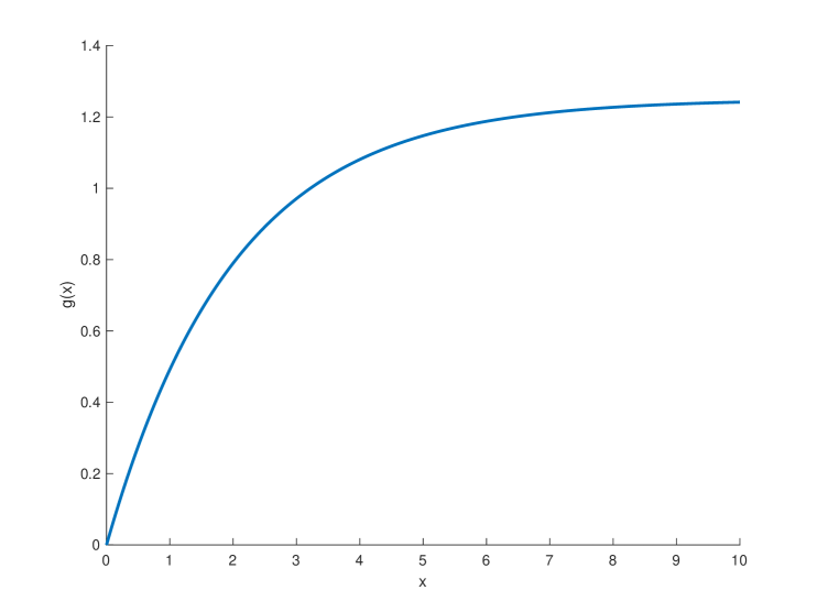
Figure 1: $-\bar{c}\gamma_{2}/r<1$, $\mu=0.1$, $r=0.08$, $\sigma=0.8$ and $\bar{c}=0.1$

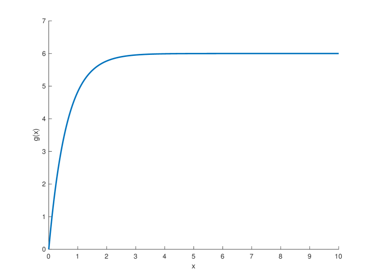
Figure 2: $-\bar{c}\gamma_{2}/r>1$, $\mu=0.4$, $r=0.05$, $\sigma=0.4$ and $\bar{c}=0.3$ and $b=1$

Proof: The estimates $0\leqslant g\leqslant\overline{c}/r$ and $0\leqslant g^{\prime}\leqslant g^{\prime}(0)<\infty$ can be easily deduced from the strictly monotonicity of $g$ and $g^{\prime}$ on ${\mathbb{R}}^{+}$. So we only need to establish the latter and $g\in C^{2}({\mathbb{R}}^{+})$ satisfies (6).

Suppose $2\mu\overline{c}\leqslant\sigma^{2}r$. Then $\overline{c}\gamma\leqslant r$, and evidently $g\in C^{2}({\mathbb{R}}^{+})$ and $g^{\prime}$ is strictly decreasing on ${\mathbb{R}}^{+}$. Since $\gamma>0$, we have

$$g^{\prime}(x)=\frac{\overline{c}\gamma}{r}e^{-\gamma x}<1,~{}~{}x>0.$$

It thus yields

$${\cal T}g=b(1-g^{\prime})+(1-b)(1-g^{\prime})^{+}=1-g^{\prime},$$

and

$$-{\cal L}g-\overline{c}{\cal T}g=-\frac{1}{2}\sigma^{2}g^{\prime\prime}-\mu g^{\prime}+rg-\overline{c}(1-g^{\prime})=0,$$

where the last equation is due to that $\gamma$ is a root for the equation

$$-\frac{1}{2}\sigma^{2}\gamma^{2}+(\mu-\overline{c})\gamma+r=0.$$

So $g$ satisfies (6). This completes the proof for the first case $\overline{c}\gamma\leqslant r$.

In the rest of the proof, we assume $2\mu\overline{c}>\sigma^{2}r$ so that $\overline{c}\gamma>r$.

We first prove that

$$\lambda_{2}k_{2}\geqslant\frac{\lambda_{1}}{\lambda_{1}+\lambda_{2}},$$ (9)

which in particular implies $k_{2}>0$. In fact, from the trivial inequality

$$\mu-\overline{c}\geqslant-\sqrt{(\mu-\overline{c})^{2}+2\sigma^{2}r}$$

we get

$$\frac{\mu-b\overline{c}}{r}\geqslant\frac{(\mu-\overline{c})-\sqrt{(\mu-\overline{c})^{2}+2\sigma^{2}r}}{2r}+\frac{(1-b)\overline{c}}{r}=\frac{(1-b)\overline{c}}{r}-\frac{1}{\gamma}.$$

Since $\lambda_{1}$ and $-\lambda_{2}$ are the two roots for the equations

$$-\frac{1}{2}\sigma^{2}\lambda^{2}-(\mu-b\overline{c})\lambda+r=0,$$

we get from the Viete theorem that

$$\frac{\lambda_{1}+(-\lambda_{2})}{\lambda_{1}(-\lambda_{2})}=\frac{\mu-b\overline{c}}{r}\geqslant\frac{(1-b)\overline{c}}{r}-\frac{1}{\gamma}.$$

This together with $\lambda_{1},\lambda_{2}>0$ gives

$$\frac{\lambda_{2}}{\lambda_{1}+\lambda_{2}}\left[1-\lambda_{1}\left(\frac{(1-b)\overline{c}}{r}-\frac{1}{\gamma}\right)\right]\geqslant\frac{\lambda_{2}}{\lambda_{1}+\lambda_{2}}\left[1-\lambda_{1}\frac{\lambda_{1}+(-\lambda_{2})}{\lambda_{1}(-\lambda_{2})}\right]=\frac{\lambda_{1}}{\lambda_{1}+\lambda_{2}},$$

which gives the desired inequality (9).

We next prove the existence of $y_{0}$. Write

$$f(y)=k_{1}e^{-\lambda_{1}y}-k_{2}e^{\lambda_{2}y}+\frac{b\overline{c}}{r}.$$ (10)

Since $\lambda_{1},\lambda_{2},k_{2}>0$ and $\lambda_{1}k_{1}+\lambda_{2}k_{2}=1$, it follows

$$f^{\prime}(y) =-\lambda_{1}k_{1}e^{-\lambda_{1}y}-\lambda_{2}k_{2}e^{\lambda_{2}y}\leqslant-\lambda_{1}k_{1}e^{-\lambda_{1}y}-\lambda_{2}k_{2}e^{-\lambda_{1}y}=-e^{-\lambda_{1}y}<0,~{}~{}y\geqslant 0.$$

Thanks to $\lambda_{1},\lambda_{2},k_{2}>0$, we have $f(+\infty)=-\infty$; and thanks to $\overline{c}\gamma>r$,

$$f(0) =k_{1}-k_{2}+\frac{b\overline{c}}{r}=\frac{\overline{c}}{r}-\frac{1}{\gamma}>0.$$

Hence, $f$ admits unique positive root $y_{0}$ in ${\mathbb{R}}^{+}$.

By the definitions of $y_{0}$ and $g$, we have $g(0)=0.$ Because

$$k_{1}-k_{2}+\frac{b\overline{c}}{r}=\frac{\overline{c}}{r}-\frac{1}{\gamma},\quad\lambda_{1}k_{1}+\lambda_{2}k_{2}=1,$$

we see that $g$ and $g^{\prime}$ are continuous at $y_{0}$, and so are on ${\mathbb{R}}^{+}$. In particular, $g^{\prime}(y_{0})=1$.

Using the same argument for the previous case, one can show that $g$ satisfies (6) on $[y_{0},\infty)$ and clearly $g^{\prime}$ is strictly decreasing there. We now show that the same properties hold on $(0,y_{0})$ too. Using the fact that $\lambda_{1}$ and $-\lambda_{2}$ are the roots for the equations

$$-\frac{1}{2}\sigma^{2}\lambda^{2}-(\mu-b\overline{c})\lambda+r=0,$$

one can show that

$$-\frac{1}{2}\sigma^{2}g^{\prime\prime}-\mu g^{\prime}+rg-b\overline{c}(1-g^{\prime})=0,~{}~{}x\in[0,y_{0}].$$ (11)

We now suppose that $g^{\prime}$ is strictly decreasing on $(0,y_{0})$, then since $g^{\prime}(y_{0})=1$, we have $g^{\prime}\geqslant 1$ on $[0,y_{0}]$, which together with (11) implies that $g$ satisfies (6).

To show that $g^{\prime}$ is strictly decreasing on $(0,y_{0})$, we fix arbitrary $x$ and $y$ such that $0<x<y<y_{0}$. Then $e^{-\lambda_{2}t}>1>e^{\lambda_{1}t}$ for any $t\in(x-y_{0},y-y_{0})$, so

$$\frac{e^{-\lambda_{2}(x-y_{0})}-e^{-\lambda_{2}(y-y_{0})}}{\lambda_{2}}=\int_{x-y_{0}}^{y-y_{0}}e^{-\lambda_{2}t}{\rm d}t>\int_{x-y_{0}}^{y-y_{0}}e^{\lambda_{1}t}{\rm d}t=\frac{e^{\lambda_{1}(y-y_{0})}-e^{\lambda_{1}(x-y_{0})}}{\lambda_{1}}.$$

After rearrangement it reads

$$\frac{\lambda_{1}}{\lambda_{2}}>\frac{e^{\lambda_{1}(y-y_{0})}-e^{\lambda_{1}(x-y_{0})}}{e^{-\lambda_{2}(x-y_{0})}-e^{-\lambda_{2}(y-y_{0})}},$$

which yields

$$\frac{\lambda_{1}}{\lambda_{1}+\lambda_{2}}>\frac{e^{\lambda_{1}(y-y_{0})}-e^{\lambda_{1}(x-y_{0})}}{e^{-\lambda_{2}(x-y_{0})}-e^{-\lambda_{2}(y-y_{0})}+e^{\lambda_{1}(y-y_{0})}-e^{\lambda_{1}(x-y_{0})}}.$$

Recalling the inequality (9), we deduce

$$\lambda_{2}k_{2}>\frac{e^{\lambda_{1}(y-y_{0})}-e^{\lambda_{1}(x-y_{0})}}{e^{-\lambda_{2}(x-y_{0})}-e^{-\lambda_{2}(y-y_{0})}+e^{\lambda_{1}(y-y_{0})}-e^{\lambda_{1}(x-y_{0})}}.$$

This can also be rewritten as

$$(1-\lambda_{2}k_{2})(e^{\lambda_{1}(x-y_{0})}-e^{\lambda_{1}(y-y_{0})})+\lambda_{2}k_{2}(e^{-\lambda_{2}(x-y_{0})}-e^{-\lambda_{2}(y-y_{0})})>0.$$

Since $\lambda_{1}k_{1}+\lambda_{2}k_{2}=1$, it follows

$$\lambda_{1}k_{1}(e^{\lambda_{1}(x-y_{0})}-e^{\lambda_{1}(y-y_{0})})+\lambda_{2}k_{2}(e^{-\lambda_{2}(x-y_{0})}-e^{-\lambda_{2}(y-y_{0})})>0,$$

leading to

$$g^{\prime}(x)=\lambda_{1}k_{1}e^{\lambda_{1}(x-y_{0})}+\lambda_{2}k_{2}e^{-\lambda_{2}(x-y_{0})}>\lambda_{1}k_{1}e^{\lambda_{1}(y-y_{0})}+\lambda_{2}k_{2}e^{-\lambda_{2}(y-y_{0})}=g^{\prime}(y).$$

This confirms that $g^{\prime}$ is strictly decreasing on $(0,y_{0})$.

Finally, since $g$ and $g^{\prime}$ are continuous and $g$ satisfies (6) on ${\mathbb{R}}^{+}$, we conclude that $g\in C^{2}({\mathbb{R}}^{+})$. This completes the proof. $\Box$

Combining Proposition 3.1 and Lemma 3.4, we conclude the following.

Theorem 3.5 (Optimal value and optimal strategy in the boundary case)

The optimal value to the problem (3) is $g$ defined in Lemma 3.4, i.e.,

$$V(x,\overline{c})=g(x),~{}~{}x\in{\mathbb{R}}^{+}.$$

which, in particular, implies that $V(x,\overline{c})$ is concave in $x$. Moreover, an optimal dividend payout strategy is given by $\{\mathcal{C}^{*}_{t}\}_{t\geqslant 0}$, where $\mathcal{C}^{*}_{t}\equiv\overline{c}$ if $2\mu\overline{c}\leqslant\sigma^{2}r$; and otherwise,

$$\mathcal{C}^{*}_{t}=\begin{cases}\overline{c}&\hbox{\; if\; $X_{t}\geqslant y_{0}$};\\ b\overline{c}&\hbox{\; otherwise.\;}\end{cases}$$ (12)

Economically speaking, since one cannot increase the value of the running maximum in the boundary case, so it is fixed. In this case, one should pay dividends at the maximum rate if the market risk is relative high (i.e., $2\mu\overline{c}/r\leqslant\sigma^{2}$) or equivalent the maximum rate is relatively small (i.e., $\overline{c}\leqslant\sigma^{2}r/(2\mu)$). The optimal strategy does not relay on the surplus level. On the other hand, if the market risk is low (i.e., $2\mu\overline{c}/r>\sigma^{2}$) or equivalent the maximum rate is relatively big (i.e., $\overline{c}>\sigma^{2}r/(2\mu)$), then the optimal strategy depends on the surplus level. One should pay dividends either at the maximum rate $\overline{c}$ if the surplus level is relative high (i.e., $X_{t}\geqslant y_{0}$), or at the minimum possible rate $b\overline{c}$ if the surplus level is relative low (i.e., $X_{t}<y_{0}$).

We now turn to the general case, which is divided into a simple case: $2\mu\overline{c}\leqslant\sigma^{2}r$, and the reminder complicated case: $2\mu\overline{c}>\sigma^{2}r$. In the former case, we will give an explicit optimal value and optimal strategy. In the latter case, the problem becomes complicated and no explicit solution or strategy is available.

4 The simple case: $2\mu\overline{c}\leqslant\sigma^{2}r$

We first solve the simple case: $2\mu\overline{c}\leqslant\sigma^{2}r$. Similar to the boundary case, we can deduce the following explicit optimal value and optimal strategy.

Theorem 4.1 (Explicit optimal value and optimal strategy in the simple case)

Suppose $2\mu\overline{c}\leqslant\sigma^{2}r$. Then the optimal value to the problem (4) is

$$V(x,c)=\frac{\overline{c}}{r}(1-e^{-\gamma x}),~{}~{}(x,c)\in{\cal Q},$$

and an optimal dividend payout strategy is given by $\{\mathcal{C}^{*}_{t}\}_{t\geqslant 0}$, where $\mathcal{C}^{*}_{t}\equiv\overline{c}$.

Proof: If $2\mu\overline{c}\leqslant\sigma^{2}r$, then $\overline{c}\gamma\leqslant r$ and $g^{\prime}\leqslant 1$ by Lemma 3.3. Therefore, for any strategy $\{\mathcal{C}_{t}\}_{t\geqslant 0}\in\Pi_{[c,\overline{c}]}$, we have

$${\cal L}g(X_{t})-g^{\prime}(X_{t})\mathcal{C}_{t}+\mathcal{C}_{t} \leqslant{\cal L}g(X_{t})+\sup\limits_{0\leqslant\mathcal{C}\leqslant\overline{c}}\mathcal{C}(1-g^{\prime}(X_{t}))$$

$$={\cal L}g(X_{t})+\overline{c}(1-g^{\prime}(X_{t}))={\cal L}g(X_{t})+\overline{c}{\cal T}g(X_{t})=0.$$

Repeating the proof of Proposition 3.1 with (8) replaced by the above inequality, one can prove the claim. $\Box$
Note that the value function in the simple case is invariant with respect $c$, i.e., $V(x,c)=V(x,\overline{c})$ for all $(x,c)\in{\cal Q}$.

In the rest of the paper, we deal with the more complicated case: $2\mu\overline{c}>\sigma^{2}r$.

5 The complicated case: $2\mu\overline{c}>\sigma^{2}r$

From now on we study the complicated case: $2\mu\overline{c}>\sigma^{2}r$, which is henceforth assumed. We will adopt a novel PDE argument plus stochastic analysis method to tackle the problem.

Our analysis consists of several parts. We start with introducing the HJB equation for the problem (4). The second step is the key of approach, where we introduce and study a regime switching system, a sequence of ODEs (where are indeed single-obstacle problems), whose solvability can be established easily by standard PDE theory. In the next step, we establish a lot of estimates for the solution of the regime switching system and construct a solution to the HJB equation of the original problem (4) from the solution of the regime switching system. Also, we propose an optimal dividend payout strategy depending on some free boundaries arising from the HJB equation. The last step is to verify that the constructed solution to the HJB equation is the value function and the proposed strategy is optimal.

We introduce the following variational inequality on $v(x,c)$:

$$\begin{cases}\min\{-{\cal L}v-c{\cal T}v,\;-v_{c}\}=0,&\hbox{in }\;{\cal Q},\\[8.53581pt] v(0,c)=0,&c\in[0,\overline{c}],\\[8.53581pt] v(x,\overline{c})=g(x),&x\in{\mathbb{R}}^{+},\end{cases}$$ (13)

It is indeed the HJB equation for our problem (4). We will show its solution is the value function of (4). The exact meaning of its solution is given as follows.

Denote ${\cal Q}_{0}={\mathbb{R}}^{+}\times[0,\overline{c})$ and

$${\cal A}=\Big{\{}v:{\cal Q}\mapsto{\mathbb{R}}\;\Big{|}\; v\in C({\cal Q}),~{}\mbox{$v$ is non-increasing w.r.t. $c$,}\;$$

$$v(\cdot,c)\in W^{2}_{p,\rm loc}({\mathbb{R}}^{+})\cap L^{\infty}({\mathbb{R}}^{+})~{}\mbox{for each}~{}c\in[0,\overline{c}]\Big{\}}.$$

Definition 5.1

We call $v$ is a solution to (13) if the follows hold:

1. $v\in{\cal A}$;

2. $v$ satisfies the boundary conditions in (13);

3. for each $c\in[0,\overline{c}]$,

   $$-{\cal L}v(\cdot,c)-c{\cal T}v(\cdot,c)\geqslant 0~{}\hbox{a.e. in}~{}{\mathbb{R}}^{+};$$ (14)

4. if there is some $(x,c)\in{\cal Q}_{0}$ such that $v(x,c)>v(x,s)$ holds for all $s\in(c,\overline{c}]$, then

   $$-{\cal L}v(y,c)-c{\cal T}v(y,c)=0~{}\hbox{for all}~{}y\in[0,x].$$ (15)

Theorem 5.2 and Theorem 5.7 will provide a complete answer to the problem (4) in the complicated case. The former resolves the solvability issue of the HJB equation (13) and establishes some properties of its solution. The latter gives the optimal value and optimal strategy for the problem.

Theorem 5.2

The equation (13) admits a unique solution $v$ in the sense of Definition 5.1. Furthermore, we have $v_{x}$ is continuous in ${\cal Q}$ and $v$ is Lipschitz continuous w.r.t. $c$, also given any $p>1$ and $\alpha=1-1/p$, there is a constant $K>0$ such that

$$0\leqslant-v_{c}\leqslant K~{}\mbox{a.e.},$$ (16)

$$0\leqslant v\leqslant\frac{\overline{c}}{r},$$ (17)

$$0\leqslant v_{x}\leqslant K,$$ (18)

and for any $(x,c)\in{\cal Q}$ and $N\in{\mathbb{N}}$,

$$v_{x}(y,c)\leqslant\max\{v_{x}(x,c),1\},~{}~{}\forall\;y\geqslant x,$$ (19)

and

$$|v(\cdot,c)|_{W^{2}_{p}[N-1,N]}+|v(\cdot,c)|_{C^{1+\alpha}({\mathbb{R}}^{+})}\leqslant K.$$ (20)

This result will be proved in Section 5.3. In the rest part of this section, we let $v$ denote the unique solution to (13), given in Theorem 5.2.

To derive the optimal strategy, our initiative thinking is as follows. On one hand, we hope to pay dividend as much as possible to increase the objective in (4), the total discounted dividend payouts. But this may lead to two unfavorable results: first, it may increase the running maximum so that shrinking the set of admissible strategies given by (3) in the future and decreasing the value function; second, the ruin time may come earlier. To avoid these negative impacts, our strategy is to increase the running maximum to some higher level only when the value functions coincide at these two levels. This motives us to define the following switching region

$$\SS=\Big{\{}(x,c)\in{\cal Q}_{0}\;\Big{|}\;v(x,c)=v(x,s)\text{ for some $s\in(c,\overline{c}]$}\Big{\}}.$$

In this region, if we increase the running maximum from $c$ to $s$, the value function will not change. Since $v$ is non-increasing in $c$, the complement of $\SS$ in ${\cal Q}_{0}$, called the non-switching region, is given by

$${\cal NS}=\Big{\{}(x,c)\in{\cal Q}_{0}\;\Big{|}\;v(x,c)>v(x,s)\text{ for all $s\in(c,\overline{c}]$}\Big{\}}.$$

In this region, increasing the running maximum is harmful, so one should not do that; in other words, one should not pay dividends exceeding the running maximum. In particular, we have (15) holds if $(x,c)\in{\cal NS}.$

It is nature to conjecture that one shall increase the running maximum only when his wealth is high enough. This motives us to define the switching boundary as follows:

$$\mathscr{X}(c)=\inf\Big{\{}x\in{\mathbb{R}}^{+}\;\Big{|}\;(x,c)\in\SS\Big{\}},~{}~{}c\in[0,\overline{c}),$$ (21)

with the convention that $\inf\emptyset=+\infty$. Clearly it holds that $\mathscr{X}(c)\leqslant x$ if $(x,c)\in\SS$. The following result shows that the reverse statement is almost true.

Proposition 5.3

The switching boundary $\mathscr{X}(\cdot)$ is positive, bounded and continuous on $[0,\overline{c})$. The limit $\mathscr{X}(\overline{c}):=\lim_{c\to\overline{c}-}\mathscr{X}(c)$ exits and is finite. Also, if $(x,c)\in\SS$, then $(y,c)\in\SS$ for any $y\geqslant x$. As a consequence, the switching and non-switching regions $\SS$ and ${\cal NS}$ are separated by $\mathscr{X}(\cdot)$:

$$\Big{\{}(x,c)\in{\cal Q}_{0}\;\Big{|}\;x>\mathscr{X}(c)\Big{\}}\subseteq\SS\subseteq\Big{\{}(x,c)\in{\cal Q}_{0}\;\Big{|}\;x\geqslant\mathscr{X}(c)\Big{\}},$$

$$\Big{\{}(x,c)\in{\cal Q}_{0}\;\Big{|}\;x<\mathscr{X}(c)\Big{\}}\subseteq{\cal NS}\subseteq\Big{\{}(x,c)\in{\cal Q}_{0}\;\Big{|}\;x\leqslant\mathscr{X}(c)\Big{\}}.$$

These properties will be proved in Section 5.4.

Remark 5.4

We do not know whether $\big{\{}(x,c)\in{\cal Q}_{0}\;\big{|}\;x=\mathscr{X}(c)\big{\}}$ belongs to $\SS$ or ${\cal NS}$. But we have the following equivalencies:

• $\mathscr{X}(\cdot)$ is non-decreasing if and only if $\big{\{}(x,c)\in{\cal Q}_{0}\;\big{|}\;x=\mathscr{X}(c)\big{\}}\in{\cal NS}$.

• $\mathscr{X}(\cdot)$ is non-increasing if and only if $\big{\{}(x,c)\in{\cal Q}_{0}\;\big{|}\;x=\mathscr{X}(c)\big{\}}\in\SS$.

Indeed, we conjecture that $\mathscr{X}(\cdot)$ is non-decreasing, which is consistent with numerical examples. Unfortunately, we cannot confirm this in theory unless $b=1$ which is proved in [22].

In order to find the optimal strategy, we define the equivalent maximum rate as

$$\mathfrak{M}(x,c)=\max\Big{\{}s\in[0,\overline{c}]\;\Big{|}\;v(x,s)=v(x,c)\Big{\}}\in[c,\overline{c}],~{}~{}(x,c)\in{\cal Q},$$

and the equivalent minimum rate as

$$\mathfrak{m}(x,c)=\min\Big{\{}s\in[0,\overline{c}]\;\Big{|}\;v(x,s)=v(x,c)\Big{\}}\in[0,c],~{}~{}(x,c)\in{\cal Q}.$$

For $(x,c)\in{\cal Q}_{0}$, the following facts can be easily verified:

• $\mathfrak{m}(x,c)\leqslant c\leqslant\mathfrak{M}(x,c)$;

• If $s\in[\mathfrak{m}(x,c),\mathfrak{M}(x,c)]$, then $v(x,s)=v(x,c)$, $\mathfrak{m}(x,s)=\mathfrak{m}(x,c)$, $\mathfrak{M}(x,s)=\mathfrak{M}(x,c)$;

• If $\mathfrak{m}(x,c)<\mathfrak{M}(x,c)$, then $(x,s)\in\SS$ for $s\in[\mathfrak{m}(x,c),\mathfrak{M}(x,c))$;

• If $\mathfrak{m}(x,c)=\mathfrak{M}(x,c)$, then $(x,c)\in{\cal NS}$;

• If $\mathfrak{M}(x,c)<\overline{c}$, then $(x,\mathfrak{M}(x,c))\in{\cal NS}$;

• $(x,c)\in\SS$ if and only if $\mathfrak{M}(x,c)>c$;

• $(x,c)\in{\cal NS}$ if and only if $\mathfrak{M}(x,c)=c$.

Given a wealth level $x$, we can increase the running maximum dividend rate $c$ to its equivalent maximum rate $\mathfrak{M}(x,c)$, which is the maximum dividend rate that will not reduce the optimal value. In particular, if $\mathfrak{M}(x,c)=c$, then one should not increase the running maximum dividend rate at this wealth level $x$. Also if $\mathfrak{M}(x,c)=\overline{c}$, then the optimal value of the problem (4) is known since $v(x,c)=v(x,\overline{c})=g(x)$.

The following result, which characterizes the equivalent maximum rate, will play a critical role in finding an optimal strategy for the problem (4).

Proposition 5.5

For each $c\in[0,\overline{c})$, $x\mapsto\mathfrak{M}(x,c)$ is non-decreasing and $x\mapsto\mathfrak{m}(x,c)$ is non-increasing on ${\mathbb{R}}^{+}$. Also, for $(x,c)\in{\cal Q}_{0}$, it holds that

$$\mathscr{X}\big{(}\mathfrak{M}(x,c)\big{)} =x \mathfrak{m}(x,c)<\mathfrak{M}(x,c)<\overline{c}$$ if ; (22)

$$-{\cal L}v\big{(}y,\mathfrak{M}(x,c)\big{)}-\mathfrak{M}(x,c){\cal T}v\big{(}y,\mathfrak{M}(x,c)\big{)} =0 \hbox{if }\;0\leqslant y\leqslant x;\vskip 3.0pt plus 1.0pt minus 1.0pt$$ (23)

$$-{\cal L}v\big{(}y,\mathfrak{m}(x,c)\big{)}-\mathfrak{m}(x,c){\cal T}v\big{(}y,\mathfrak{m}(x,c)\big{)} =0 \hbox{if }\;0\leqslant y\leqslant x\mbox{ and }\mathfrak{m}(x,c)>0;\vskip 3.0pt plus 1.0pt minus 1.0pt$$ (24)

$$\lim\limits_{y\to x+}\mathfrak{M}(y,c) =\mathfrak{M}(x,c);\vskip 3.0pt plus 1.0pt minus 1.0pt$$ (25)

$$\lim\limits_{y\to x+}\mathfrak{m}(y,c) =\mathfrak{m}(x,c);$$ (26)

$$v_{c}(x,s) =0 \hbox{if }\mathfrak{m}(x,c)<s\leqslant\mathfrak{M}(x,c)<\overline{c}.$$ (27)

Also,

$$\SS=\Big{\{}(x,s)\;\Big{|}\;\mathfrak{m}(x,c)\leqslant s<\mathfrak{M}(x,c),~{}(x,c)\in{\cal Q}_{0}\Big{\}}.$$

These properties will be proved in Section 5.5. Below is an demonstration figure.

Figure 3: The value functions $c\mapsto v(x_{i},c)$ are in solid curve, from below to top corresponding to $x_{1}<x_{2}<x_{3}<x_{4}$. The dashed curve is $\mathscr{X}(\cdot)$. Its blue parts stand for $\mathfrak{m}(x,c_{1})$ and $\mathfrak{m}(x,c_{2})$ at all different levels of $x$, whereas the red parts stand for $\mathfrak{M}(x,c_{1})$ and $\mathfrak{M}(x,c_{2})$. If a point belongs to $\SS$ (resp. ${\cal NS}$), then so does any point above (resp. below) it. Hence, all points above (resp. below) dashed curve belong to $\SS$ (resp. ${\cal NS}$). The blue (resp. red) parts of the dashed curve belong to $\SS$ (resp. ${\cal NS}$). Therefore, the blue parts are expending as $x$ gets bigger and eventually the whole curve becomes blue above certain threshold (which is indeed $\sup_{c\in[0,\overline{c})}\mathscr{X}(c)$). Although the dashed curve in above demonstration figure is $W$-shaped, we believe it should be increasing as $c$ gets bigger. Unfortunately, we cannot prove this, but numerical examples in Section 5.1 strongly support our conjecture.

On the other hand, the objective is linear in the dividend payout, so one may expect a bang-bang dividend payout strategy: paying dividend at the maximum possible rate if the surplus is relatively high; at the minimum rate otherwise. If the marginal utility is bigger than one, then one should keep the surplus as high as possible to wait for a better future, so one should save money and pay dividend at the minimum possible rate; otherwise, at the maximum rate. The above thinking motives us to define the following minimum dividend payout region

$${\cal D}_{\min}=\Big{\{}(x,c)\in{\cal Q}\;\Big{|}\;v_{x}(x,c)>1\Big{\}},$$

and the maximum dividend payout region

$${\cal D}_{\max}=\Big{\{}(x,c)\in{\cal Q}\;\Big{|}\;v_{x}(x,c)\leqslant 1\Big{\}}.$$

These two regions will be separated by the following converting boundary

$$\mathscr{Y}(c)=\inf\Big{\{}x\in{\mathbb{R}}^{+}\;\Big{|}\;v_{x}(x,c)\leqslant 1\Big{\}},~{}~{}c\in[0,\overline{c}].$$ (28)

The following result characterizes the converting boundary.

Proposition 5.6

The converting boundary $\mathscr{Y}(\cdot)$ is continuous on $[0,\overline{c}]$, and satisfies $\mathscr{Y}(\overline{c})=y_{0}$, $v_{x}(\mathscr{Y}(c),c)=1$, and

$$0<\mathscr{Y}(c)<\mathscr{X}(c),~{}~{}c\in[0,\overline{c}].$$ (29)

Also, it separates the minimum and the maximum dividend payout regions ${\cal D}_{\min}$ and ${\cal D}_{\max}$:

$${\cal D}_{\min} =\Big{\{}(x,c)\in{\cal Q}\;\Big{|}\;x<\mathscr{Y}(c)\Big{\}},~{}~{}{\cal D}_{\max}=\Big{\{}(x,c)\in{\cal Q}\;\Big{|}\;x\geqslant\mathscr{Y}(c)\Big{\}}.$$

Using the above results, we now give the optimal value and the optimal strategy for the problem (4) in the complicated case as follows.

Theorem 5.7 (Optimal value and optimal strategy in the complicated case.)

Let $v$ be the unique solution to (13), given in Theorem 5.2. Then it coincides with the optimal value to the problem (4). Moreover, $\{\mathcal{C}^{*}_{t}\}_{t\geqslant 0}$ is an optimal strategy for the problem (4) with $(x,c)\in{\cal Q}_{0}$, where the triple $(X^{*}_{t},\mathcal{M}^{*}_{t},\mathcal{C}^{*}_{t})$ is determined by

$$\begin{cases}\displaystyle{X^{*}_{t}=x+\int_{0}^{t}(\mu-\mathcal{C}^{*}_{s}){\rm d}s+\int_{0}^{t}\sigma{\rm d}W_{s},}\\[14.22636pt] \mathcal{M}^{*}_{t}=\mathfrak{M}\Big{(}\max\limits_{s\in[0,t]}X^{*}_{s},c\Big{)},\\[14.22636pt] \mathcal{C}^{*}_{t}=\Big{(}b+(1-b)1_{\{X^{*}_{t}\geqslant\mathscr{Y}(\mathcal{M}^{*}_{t})\}}\Big{)}\mathcal{M}^{*}_{t}.\end{cases}$$

Proof: Suppose $V(x,c)$ is the value function defined in (4) and $v(x,c)$ is the solution to (13). We come to prove $v(x,c)=V(x,c)$.

For any $(x,c)\in{\cal Q}_{0}$, any admissible dividend payout strategy $\{\mathcal{C}_{t}\}_{t\geqslant 0}\in\Pi_{[c,\overline{c}]}$ and any constant $T>0$, through a change of measure argument, one can show that $X_{t}$ is a Brownian motion under some equivalent probability measure, so $\int_{0}^{T}{\mathbb{P}}(X_{t}\in K){\rm d}t=0$ for any subset $K$ of ${\mathbb{R}}$ with zero Lebesgue measure.

Applying Itô’s formula (see [25] Theorem 33 on page 81) to $e^{-rt}v(X_{t},\mathcal{M}_{t})$ and then taking expectation lead to

$$v(x,c) ={\mathbb{E}}\Bigg{[}e^{-r(\tau\wedge T)}v(X_{\tau\wedge T},\mathcal{M}_{\tau\wedge T})+\int_{0}^{\tau\wedge T}e^{-rt}\Big{(}-{\cal L}v(X_{t},\mathcal{M}_{t})+v_{x}(X_{t},\mathcal{M}_{t})\mathcal{C}_{t}\Big{)}{\rm d}t$$

$$\qquad\quad-\sum_{0\leqslant t\leqslant\tau\wedge T}e^{-rt}\Big{(}v(X_{t},\mathcal{M}_{t})-v(X_{t},\mathcal{M}_{t-})\Big{)}-\int_{0}^{\tau\wedge T}e^{-rt}v_{c}(X_{t},\mathcal{M}_{t}){\rm d}\mathcal{M}^{c}_{t}$$

$$\qquad\quad-\int_{0}^{\tau\wedge T}e^{-rt}\sigma v_{x}(X_{t},\mathcal{M}_{t}){\rm d}W_{t}\;\Bigg{|}\;X_{0}=x,~{}\mathcal{M}_{0}=c\Bigg{]},$$

where $\mathcal{M}_{t}^{c}$ is the continuous part of $\mathcal{M}_{t}$. The mean of the stochastic integral is zero since the integrand is bounded. Applying (13), we get

$$-{\cal L}v(X_{t},\mathcal{M}_{t})+v_{x}(X_{t},\mathcal{M}_{t})\mathcal{C}_{t}-\mathcal{C}_{t}\geqslant -{\cal L}v(X_{t},\mathcal{M}_{t})-\sup\limits_{b\mathcal{M}_{t}\leqslant\mathcal{C}\leqslant\mathcal{M}_{t}}\mathcal{C}(1-v_{x}(X_{t},\mathcal{M}_{t}))$$

$$= -{\cal L}v(X_{t},\mathcal{M}_{t})-\mathcal{M}_{t}{\cal T}v(X_{t},\mathcal{M}_{t})\geqslant 0.$$

Together with

$$-v_{c}\geqslant 0,\quad M_{t}\geqslant M_{t-},\quad{\rm d}\mathcal{M}^{c}_{t}\geqslant 0,$$

we have

$$v(x,c)\geqslant{\mathbb{E}}\Bigg{[}e^{-r(\tau\wedge T)}v(X_{\tau\wedge T},\mathcal{M}_{\tau\wedge T})+\int_{0}^{\tau\wedge T}e^{-rt}\mathcal{C}_{t}{\rm d}t\;\Bigg{|}\;X_{0}=x,~{}\mathcal{M}_{0}=c\Bigg{]}.$$ (30)

Because $v$, $\mathcal{C}_{t}\geqslant 0$, dropping the first term in the expectation and sending $T\to+\infty$ in above, the monotone convergence theorem gives

$$v(x,c)\geqslant{\mathbb{E}}\Bigg{[}\int_{0}^{\tau}e^{-rt}\mathcal{C}_{t}{\rm d}t\;\Bigg{|}\;X_{0}=x,~{}\mathcal{M}_{0}=c\Bigg{]}.$$

Since $\{\mathcal{C}_{t}\}_{t\geqslant 0}\in\Pi_{[c,\overline{c}]}$ is arbitrary selected, we obtain $v(x,c)\geqslant V(x,c)$.

We now prove the opposite inequality $v(x,c)\leqslant V(x,c),$ and show that $\{\mathcal{C}^{*}_{t}\}_{t\geqslant 0}$ is an optimal strategy. Thanks to the continuity of $X^{*}$ and $\mathscr{Y}(\cdot)$, the right-continuity of $\mathcal{M}^{*}$ given by (25), it is not hard to verify $\{\mathcal{C}^{*}_{t}\}_{t\geqslant 0}\in\Pi_{[c,\overline{c}]}$ is an admissible strategy.

We now assume $t\in[0,\zeta_{1})$, where $\zeta_{1}$ is a stopping time given by

$$\zeta_{1}=\sup\big{\{}t\geqslant 0\;\big{|}\;\mathcal{M}^{*}_{t}\leqslant c\big{\}}.$$

Since $\mathcal{M}^{*}_{0}=c$, we have $\mathcal{M}^{*}_{t}=c$. It follows

$$\mathfrak{M}\Big{(}\max\limits_{s\in[0,t]}X^{*}_{s},c\Big{)}=\mathcal{M}^{*}_{t}=c,$$

and

$$\Big{(}\max\limits_{s\in[0,t]}X^{*}_{s},c\Big{)}\in{\cal NS}.$$

It follows from (15) that

$$-{\cal L}v(y,c)-c{\cal T}v(y,c)=0~{}\hbox{for all }\;y\in\Big{[}0,\max\limits_{s\in[0,t]}X^{*}_{s}\Big{]},$$ (31)

which, in particular, yields

$$-{\cal L}v(X^{*}_{t},\mathcal{M}^{*}_{t})-\mathcal{M}^{*}_{t}{\cal T}v(X^{*}_{t},\mathcal{M}^{*}_{t}) =-{\cal L}v(X^{*}_{t},c)-c{\cal T}v(X^{*}_{t},c)=0.$$

By the construction of $\mathcal{C}^{*}_{t}$, it gives

$$-{\cal L}v(X^{*}_{t},\mathcal{M}^{*}_{t})+\mathcal{C}^{*}_{t}v_{x}(X^{*}_{t},\mathcal{M}^{*}_{t})-\mathcal{C}^{*}_{t} =-{\cal L}v(X^{*}_{t},\mathcal{M}^{*}_{t})-\mathcal{M}^{*}_{t}{\cal T}v(X^{*}_{t},\mathcal{M}^{*}_{t})=0.$$

Now applying Itô’s formula to $e^{-rt}v(X^{*}_{t},c)$ on $[0,\zeta_{1}\wedge\tau\wedge T)$ gives

$$v(x,c) ={\mathbb{E}}\Bigg{[}e^{-r(\zeta_{1}\wedge\tau\wedge T)}v(X^{*}_{\zeta_{1}\wedge\tau\wedge T},c)+\int_{0}^{\zeta_{1}\wedge\tau\wedge T}e^{-rt}\Big{(}-{\cal L}v(X^{*}_{t},c)+\mathcal{C}^{*}_{t}v_{x}(X^{*}_{t},c)\Big{)}{\rm d}t$$

$$\qquad\quad-\int_{0}^{\zeta_{1}\wedge\tau\wedge T}e^{-rt}\sigma v_{x}(X^{*}_{t},c){\rm d}W_{t}\;\Bigg{|}\;X_{0}=x,~{}\mathcal{M}_{0}=c\Bigg{]}$$

$$={\mathbb{E}}\Bigg{[}e^{-r(\zeta_{1}\wedge\tau\wedge T)}v\big{(}X^{*}_{\zeta_{1}\wedge\tau\wedge T},\mathcal{M}^{*}_{(\zeta_{1}-)\wedge\tau\wedge T}\big{)}$$

$$\qquad\quad+\int_{0}^{\zeta_{1}\wedge\tau\wedge T}e^{-rt}\Big{(}-{\cal L}v(X^{*}_{t},\mathcal{M}^{*}_{t})+\mathcal{C}^{*}_{t}v_{x}(X^{*}_{t},\mathcal{M}^{*}_{t})\Big{)}{\rm d}t\;\Bigg{|}\;X_{0}=x,~{}\mathcal{M}_{0}=c\Bigg{]}\vskip 3.0pt plus 1.0pt minus 1.0pt$$

$$={\mathbb{E}}\Bigg{[}e^{-r(\zeta_{1}\wedge\tau\wedge T)}v\big{(}X^{*}_{\zeta_{1}\wedge\tau\wedge T},\mathcal{M}^{*}_{(\zeta_{1}-)\wedge\tau\wedge T}\big{)}+\int_{0}^{\zeta_{1}\wedge\tau\wedge T}e^{-rt}\mathcal{C}^{*}_{t}{\rm d}t\;\Bigg{|}\;X_{0}=x,~{}\mathcal{M}_{0}=c\Bigg{]}.$$ (32)

Now let us consider the case $t\in[\zeta_{1},\zeta_{2})$, where $\zeta_{2}$ is a stopping time defined by

$$\zeta_{2}=\inf\big{\{}t\geqslant\zeta_{1}\;\big{|}\;\mathcal{M}^{*}_{t}=\overline{c}\big{\}}.$$

We first assume $\mathcal{M}^{*}_{\zeta_{1}}>c$. Then $c<\mathcal{M}^{*}_{t}<\overline{c}$. So, by the construction of $\mathcal{C}^{*}_{t}$ and (23),

$$\quad-{\cal L}v(X^{*}_{t},\mathcal{M}^{*}_{t})+\mathcal{C}^{*}_{t}v_{x}(X^{*}_{t},\mathcal{M}^{*}_{t})-\mathcal{C}^{*}_{t}\vskip 3.0pt plus 1.0pt minus 1.0pt$$

$$=-{\cal L}v(X^{*}_{t},\mathcal{M}^{*}_{t})-\mathcal{M}^{*}_{t}{\cal T}v(X^{*}_{t},\mathcal{M}^{*}_{t})$$

$$=-{\cal L}v\Big{(}X^{*}_{t},\mathfrak{M}\Big{(}\max\limits_{s\in[0,t]}X^{*}_{s},c\Big{)}\Big{)}-\mathfrak{M}\Big{(}\max\limits_{s\in[0,t]}X^{*}_{s},c\Big{)}{\cal T}v\Big{(}X^{*}_{t},\mathfrak{M}\Big{(}\max\limits_{s\in[0,t]}X^{*}_{s},c\Big{)}\Big{)}$$

$$=0.$$

By virtue of (22),

$$\mathscr{X}(\mathcal{M}^{*}_{t})=\mathscr{X}\Big{(}\mathfrak{M}\Big{(}\max\limits_{s\in[0,t]}X^{*}_{s},c\Big{)}\Big{)}=\max\limits_{s\in[0,t]}X^{*}_{s},$$

implying

$$X^{*}_{t}\leqslant\mathscr{X}(\mathcal{M}^{*}_{t}).$$

If $X^{*}_{t}=\mathscr{X}(\mathcal{M}^{*}_{t})$, then thanks to (27), we have $v_{c}(X^{*}_{t},\mathcal{M}^{*}_{t})=0$, so

$$-v_{c}(X^{*}_{t},\mathcal{M}^{*}_{t}){\rm d}(\mathcal{M}^{*})^{c}_{t}=0.$$

If $X^{*}_{t}<\mathscr{X}(\mathcal{M}^{*}_{t})$, then ${\rm d}(\mathcal{M}^{*})^{c}_{t}=0$, so the above equation also holds. Also, if $\mathcal{M}^{*}_{t}>\mathcal{M}^{*}_{t-}$, then $X^{*}_{t}=\max\limits_{s\in[0,t]}X^{*}_{s}$, and thus

$$\mathcal{M}^{*}_{t}=\mathfrak{M}\Big{(}\max\limits_{s\in[0,t]}X^{*}_{s},c\Big{)}=\mathfrak{M}(X^{*}_{t},c).$$

Because $c\leqslant\mathcal{M}^{*}_{t-}\leqslant\mathcal{M}^{*}_{t}=\mathfrak{M}(X^{*}_{t},c)$ and $v\big{(}x,\mathfrak{M}(x,c)\big{)}=v(x,s)$ for any $s\in[c,\mathfrak{M}(x,c)]$, we get

$$v(X^{*}_{t},\mathcal{M}^{*}_{t})=v(X^{*}_{t},\mathfrak{M}(X^{*}_{t},c))=v(X^{*}_{t},\mathcal{M}^{*}_{t-}).$$

Now suppose $\mathcal{M}^{*}_{\zeta_{1}}=c$, then $\mathcal{M}^{*}_{\zeta_{1}}=c=\mathcal{M}^{*}_{\zeta_{1}-}$. It implies $\mathcal{M}^{*}_{(\zeta_{1}-)\wedge\tau\wedge T}=\mathcal{M}^{*}_{\zeta_{1}\wedge\tau\wedge T}$; and hence

$$v(X^{*}_{\zeta_{1}\wedge\tau\wedge T},\mathcal{M}^{*}_{\zeta_{1}\wedge\tau\wedge T})=v(X^{*}_{\zeta_{1}\wedge\tau\wedge T},\mathcal{M}^{*}_{(\zeta_{1}-)\wedge\tau\wedge T}).$$

Now applying Itô’s formula to $e^{-rt}v(X^{*}_{t},\mathcal{M}^{*}_{t})$ on $((\zeta_{1}-)\wedge\tau\wedge T,\zeta_{2}\wedge\tau\wedge T]$ gives

$$\quad\;{\mathbb{E}}\Big{[}e^{-r(\zeta_{1}\wedge\tau\wedge T)}v\big{(}X^{*}_{\zeta_{1}\wedge\tau\wedge T},\mathcal{M}^{*}_{(\zeta_{1}-)\wedge\tau\wedge T}\big{)}\;\Big{|}\;X_{0}=x,~{}\mathcal{M}_{0}=c\Big{]}\vskip 3.0pt plus 1.0pt minus 1.0pt$$

$$={\mathbb{E}}\Bigg{[}e^{-r(\zeta_{2}\wedge\tau\wedge T)}v\big{(}X^{*}_{\zeta_{2}\wedge\tau\wedge T},\mathcal{M}^{*}_{\zeta_{2}\wedge\tau\wedge T}\big{)}+\int_{\zeta_{1}\wedge\tau\wedge T}^{\zeta_{2}\wedge\tau\wedge T}e^{-rt}\Big{(}-{\cal L}v(X^{*}_{t},\mathcal{M}^{*}_{t})+v_{x}(X^{*}_{t},\mathcal{M}^{*}_{t})\mathcal{C}^{*}_{t}\Big{)}{\rm d}t$$

$$\qquad\quad-\sum_{\zeta_{1}\wedge\tau\wedge T\leqslant t\leqslant\zeta_{2}\wedge\tau\wedge T}e^{-rt}\Big{(}v(X^{*}_{t},\mathcal{M}^{*}_{t})-v(X^{*}_{t},\mathcal{M}^{*}_{t-})\Big{)}-\int_{\zeta_{1}\wedge\tau\wedge T}^{\zeta_{2}\wedge\tau\wedge T}e^{-rt}v_{c}(X^{*}_{t},\mathcal{M}^{*}_{t}){\rm d}(\mathcal{M}^{*})^{c}_{t}$$

$$\qquad\quad-\int_{\zeta_{1}\wedge\tau\wedge T}^{\zeta_{2}\wedge\tau\wedge T}e^{-rt}\sigma v_{x}(X^{*}_{t},\mathcal{M}^{*}_{t}){\rm d}W_{t}\;\Bigg{|}\;X_{0}=x,~{}\mathcal{M}_{0}=c\Bigg{]}\vskip 3.0pt plus 1.0pt minus 1.0pt$$

$$={\mathbb{E}}\Bigg{[}e^{-r(\zeta_{2}\wedge\tau\wedge T)}v\big{(}X^{*}_{\zeta_{2}\wedge\tau\wedge T},\mathcal{M}^{*}_{\zeta_{2}\wedge\tau\wedge T}\big{)}+\int_{\zeta_{1}\wedge\tau\wedge T}^{\zeta_{2}\wedge\tau\wedge T}e^{-rt}\mathcal{C}^{*}_{t}{\rm d}t\;\Bigg{|}\;X_{0}=x,~{}\mathcal{M}_{0}=c\Bigg{]}.$$ (33)

Finally, we assume $t\in[\zeta_{2},\tau)$, then $\mathcal{M}^{*}_{t}=\overline{c}$. We can deduce similarly to the case $t\in[0,\zeta_{1})$ to get

$$\quad\;{\mathbb{E}}\Big{[}e^{-r(\zeta_{2}\wedge\tau\wedge T)}v\big{(}X^{*}_{\zeta_{2}\wedge\tau\wedge T},\mathcal{M}^{*}_{\zeta_{2}\wedge\tau\wedge T}\big{)}\;\Big{|}\;X_{0}=x,~{}\mathcal{M}_{0}=c\Big{]}\vskip 3.0pt plus 1.0pt minus 1.0pt$$

$$={\mathbb{E}}\Bigg{[}e^{-r(\tau\wedge T)}v\big{(}X^{*}_{\tau\wedge T},\mathcal{M}^{*}_{\tau\wedge T}\big{)}+\int_{\zeta_{2}\wedge\tau\wedge T}^{\tau\wedge T}e^{-rt}\mathcal{C}^{*}_{t}{\rm d}t\;\Bigg{|}\;X_{0}=x,~{}\mathcal{M}_{0}=c\Bigg{]}.$$

Combining (32), (33) and above, we obtain

$$v(x,c) ={\mathbb{E}}\Bigg{[}e^{-r(\tau\wedge T)}v\big{(}X^{*}_{\tau\wedge T},\mathcal{M}^{*}_{\tau\wedge T}\big{)}+\int_{0}^{\tau\wedge T}e^{-rt}\mathcal{C}^{*}_{t}{\rm d}t\;\Bigg{|}\;X_{0}=x,~{}\mathcal{M}_{0}=c\Bigg{]}.$$ (34)

Because $v$ is bounded and $r>0$, it yields

$$\lim_{T\to+\infty}e^{-r(\tau\wedge T)}v\big{(}X^{*}_{\tau\wedge T},\mathcal{M}^{*}_{\tau\wedge T}\big{)}1_{\tau=+\infty}=\lim_{T\to+\infty}e^{-rT}v(X^{*}_{T},\mathcal{M}^{*}_{T})1_{\tau=+\infty}=0;$$

whereas, by virtue of $X^{*}_{\tau}1_{\tau<+\infty}=0$ and $v(0,c)=0$, it follows

$$\lim_{T\to+\infty}e^{-r(\tau\wedge T)}v\big{(}X^{*}_{\tau\wedge T},\mathcal{M}^{*}_{\tau\wedge T}\big{)}1_{\tau<+\infty}=e^{-r\tau}v(X^{*}_{\tau},\mathcal{M}^{*}_{\tau})1_{\tau<+\infty}=e^{-r\tau}v(0,\mathcal{M}^{*}_{\tau})1_{\tau<+\infty}=0.$$

Therefore, by sending $T\to+\infty$ in (34) and using the dominated and monotone convergence theorems, we obtain

$$v(x,c)={\mathbb{E}}\Bigg{[}\int_{0}^{\tau}e^{-rt}\mathcal{C}^{*}_{t}{\rm d}t\;\Bigg{|}\;X_{0}=x,~{}\mathcal{M}_{0}=c\Bigg{]}.$$

In view of the definition of $V(x,c)$, we conclude that $v(x,c)\leqslant V(x,c)$, and consequently, that $\{\mathcal{C}^{*}_{t}\}_{t\geqslant 0}$ is an optimal dividend payout strategy. $\Box$

It is left to prove Theorem 5.2, Proposition 5.3, Proposition 5.5 and Proposition 5.6. This will be a long technical journey. Before doing that, we first present our numerical study.

5.1 Numerical examples

We provide here some numerical examples with parameter values $\mu=0.3$, $r=0.05$, $\sigma=0.3$, $\bar{c}=0.3$.

We study the impact of different values of $b$ in Figures 4-7. In each figure, the switching boundary $\mathscr{X}(\cdot)$ and the converting boundary $\mathscr{Y}(\cdot)$ are shown in the left panel; whereas the corresponding value function is shown in the right panel. These figures are calculated by solving (35) in the next section.

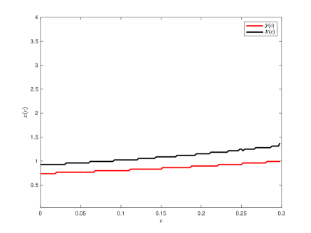
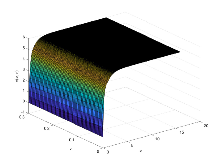
Figure 4: $b=0.4$. The free boundaries $\mathscr{X}(\cdot)$ and $\mathscr{Y}(\cdot)$ and the value function $v$

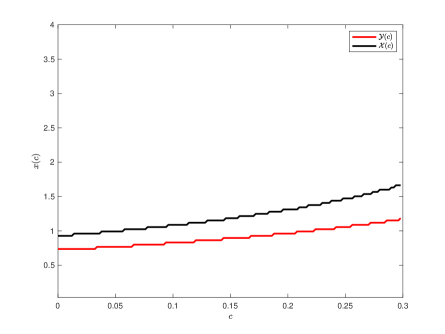
Figure 5: $b=0.6$. The free boundaries $\mathscr{X}(\cdot)$ and $\mathscr{Y}(\cdot)$ and the value function $v$

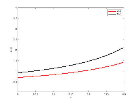
Figure 6: $b=0.8$. The free boundaries $\mathscr{X}(\cdot)$ and $\mathscr{Y}(\cdot)$ and the value function $v$

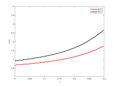
Figure 7: $b=1$. The free boundaries $\mathscr{X}(\cdot)$ and $\mathscr{Y}(\cdot)$ and the value function $v$

We can observe from Figures 4-7 that the bigger the value of $b$, the bigger the slopes of $\mathscr{X}(\cdot)$ and $\mathscr{Y}(\cdot)$. Financially speaking, a stricter drawdown constraint makes its harder to increase the maximum dividend payout rate. This is consistent with our intuition.

Figure 8 compares $\mathscr{X}(\cdot)$ and $\mathscr{Y}(\cdot)$ at difference values of $b$.

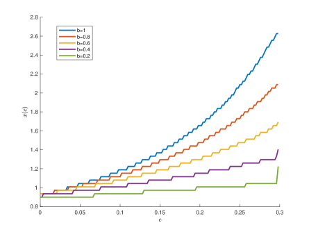
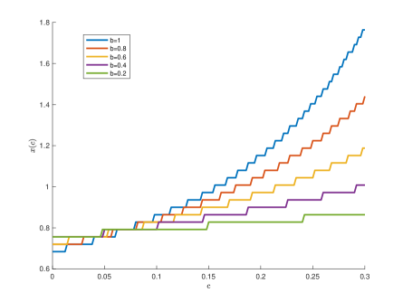
Figure 8: The free boundaries $\mathscr{X}(\cdot)$ on the left and $\mathscr{Y}(\cdot)$ on the right with various values of $b$

The left panel in Figure 8 shows that the bigger the value of $b$, the bigger the value of $\mathscr{X}(\cdot)$. It means, when the drawdown constraint becomes stricter, in order to increase the maximum dividend payout rate, one has to achieve a higher surplus level. By contrast, we see from the right panel in Figure 8 that the value of $\mathscr{Y}(\cdot)$ is not always monotonic increasing w.r.t. $b$.

Unfortunately, we cannot prove these phenomenons observed in above.

The rest of this paper is devoted to establishing Theorem 5.2, Proposition 5.3, Proposition 5.5 and Proposition 5.6.

5.2 An approximation regime switching problem

We notice that (13) is a PDE, which is generally harder to deal with than ODEs of the same order. Following Albrecher et al. [2], we reduce it to the study of a sequence of ODEs. We use a pure differential equation methods to study it, so that a better solution will be given.

Let us explain our approach in details as follows. Since $\mathcal{C}_{t}$ is increasing, the admissible strategy set is shrinking as the increasing of $\mathcal{C}_{t}$. If there are only finite discrete values for $\mathcal{C}_{t}$, one can treat the cases one by one backwardly: from a lager value to a smaller one. We have already done the first step where $\mathcal{C}_{t}$ achieves its maximum $\overline{c}$ that is the boundary case studied in Section 3. We can deal with the case where $\mathcal{C}_{t}$ is fixed as a smaller value than $\overline{c}$. Since the running maximum is fixed, the HJB equation reduces to an ODE, which can be treated similarly to the boundary case studied in Section 3. By mathematical induction, we can solve the discrete value case. Once this is done, we will take a limit argument to derive the desired solution to the original HJB equation (13).

We now realize the above idea. Suppose the dividend payout rate can only take the following discrete values

$$c_{i}=\overline{c}-i\Delta c,~{}~{}i=0,1,2,\cdots,n,$$

with $\Delta c=\overline{c}/n>0$. Let $v_{-1}=0$, we consider the following regime switching ODE system:

$$\begin{cases}\min\{-{\cal L}v_{i}-c_{i}{\cal T}v_{i},\;v_{i}-v_{i-1}\}=0,&x>0,~{}~{}i=0,1,2,\cdots,n,\\[8.53581pt] v_{i}(0)=0,&i=0,1,2,\cdots,n,\end{cases}$$ (35)

under bounded growth condition. Here, we can think of $v_{i}(x)$ as an approximation of $v(x,c_{i})$.

Clearly, the system (35) can be solved recursively: for each $i$, it is a single-obstacle ODE problem if $v_{i-1}$ is known. One could easily construct a numerical scheme (such as the standard penalty method in [17]) to generate the solution $v_{i}(x)$ to (35) given $v_{i-1}$ is known. The free boundaries $\mathscr{X}(\cdot)$ and $\mathscr{Y}(\cdot)$ can thereby be connected for all $i=1,2,...,n$ as shown in the previous section.

Lemma 5.8

The system (35) has a solution $v_{i}\in W^{2}_{p,\rm loc}({\mathbb{R}}^{+})\cap C^{1+\alpha}({\mathbb{R}}^{+}),\;i=0,1,2,\cdots,n$ for any $p>1$ and $\alpha=1-1/p,$ which satisfies

$$0\leqslant v_{i}\leqslant\frac{\overline{c}}{r},$$ (36)

$$v_{i}^{\prime}\geqslant 0,$$ (37)

and

$$v_{i}^{\prime}(y)\leqslant\max\{v_{i}^{\prime}(x),1\},\quad\forall\;0\leqslant x\leqslant y.$$ (38)

Moreover, for each $i=1,2,\cdots,n,$ there is a free boundary point $x_{i}>0$ such that $v_{i}(x)=v_{i-1}(x)$ if $x\geqslant x_{i}$ and $v_{i}(x)>v_{i-1}(x)$ if $x<x_{i}$. Also, $v^{\prime}_{i}(x)\leqslant 1$ if $x\geqslant x_{i}$.

Proof: It follows from (6), $c_{0}=\overline{c}$ and $g\geqslant 0=v_{-1}$ that

$$\begin{cases}\min\{-{\cal L}g-c_{0}{\cal T}g,\;g-v_{-1}\}=0,&x>0,\\ g(0)=0.&\end{cases}$$

Therefore, the solution to (35) if $i=0$ is $v_{0}=g$.

By the standard penalty method and $L_{p}$ theorem, we can prove

$$v_{i}\in W^{2}_{p,\rm loc}({\mathbb{R}}^{+})$$

step by step from $i=1,2,\cdots,n$. By the Sobolev embedding theorem, we also have

$$v_{i}\in C^{1+\alpha}({\mathbb{R}}^{+}),$$

since the process is standard (see, e.g., [18]), we omit the details.

From (35), we have

$$v_{i}\geqslant v_{i-1}\geqslant\cdots\geqslant v_{0}\geqslant 0,$$ (39)

so the lower bound in (36) holds. Furthermore, since $v_{i}(x)-v_{i}(0)\geqslant v_{0}(x)-v_{0}(0)=g(x)-g(0)$ for $i\geqslant 0$, it follows that $v^{\prime}_{i}(0)\geqslant g^{\prime}(0)>g^{\prime}(y_{0})=1$ by recalling that $\overline{c}\gamma>r$ and Lemma 3.4.

We now prove the remaining claims by mathematical induction. By Lemma 3.4, we have $v_{0}(x)=g(x)$ satisfies (36)-(38). Suppose all the desired results of the lemma hold for some $i=j-1$ ($1\leqslant j<n$), we are going to prove they also hold if $i=j$.

By the induction hypothesis, we have $v_{j-1}\leqslant\overline{c}/r$. It is clearly that the constant function $\overline{c}/r$ is a super solution to (35) for $v_{j}$, so $v_{j}$ also satisfies the upper bound in (36).

We now prove the set

$$E_{j}:=\{x>0\;|\;v_{j}(x)=v_{j-1}(x)\}$$

is not empty. Suppose, on the contrary it was empty, then by (35) we would have $-{\cal L}v_{j}-c_{j}{\cal T}v_{j}=0$ on ${\mathbb{R}}^{+}$. Applying the comparison principle we can prove that $v_{j}\leqslant c_{j}/r$ under the bounded growth condition and $v_{j}(0)=0$, which would lead to $v_{j}(+\infty)\leqslant c_{j}/r<\overline{c}/r=v_{0}(+\infty)$, contradicting to the order (39). Therefore, $E_{j}$ is not empty, and consequently,

$$x_{j}:=\inf E_{j}<\infty.$$

We next prove that

there is no $$x>0 v_{j}(x)=v_{j-1}(x) v_{j-1}^{\prime}(x)>1$$ such that and . (40)

Suppose, on the contrary, there is some $x>0$ such that $v_{j}(x)=v_{j-1}(x)$ and $\max\{v_{j-1}^{\prime}(x),v_{j}^{\prime}(x)\}>1$. There are two cases: either there is $1\leqslant k\leqslant j-1$ such that

$$v_{j}(x)=v_{j-1}(x)=\cdots=v_{j-k}(x)>v_{j-k-1}(x);$$

or $v_{j}(x)=v_{j-1}(x)=\cdots=v_{0}(x)$. In the former case, since $v_{j-k}$ and $v_{j-k-1}$ are continuous, there is a neighborhood $I_{\varepsilon}=(x-\varepsilon,x+\varepsilon)$ such that $v_{j-k}>v_{j-k-1}$ in $I_{\varepsilon},$ so that

$$-{\cal L}v_{j-k}-c_{j-k}{\cal T}v_{j-k}=0~{}\hbox{a.e. in }I_{\varepsilon}.$$ (41)

Whereas in the latter case, we set $k=j$ and the above equation still holds since $v_{j-k}\equiv v_{0}$.

Combining (35) and (41) yields

$$\frac{\sigma^{2}}{2}(v_{j}-v_{j-k})^{\prime\prime}\leqslant-\mu(v_{j}^{\prime}-v_{j-k}^{\prime})+r(v_{j}-v_{j-k})-c_{j}({\cal T}v_{j}-{\cal T}v_{j-k})+k\Delta c{\cal T}v_{j-k}~{}\hbox{a.e. in }I_{\varepsilon}.$$ (42)

Note that both functions $v_{j}-v_{j-k}$ and $v_{j-1}-v_{j-k}$ attain their minimum value $0$ at $x$, so

$$v_{j}(x)=v_{j-k}(x),~{}~{}v_{j}^{\prime}(x)=v_{j-k}^{\prime}(x)=v_{j-1}^{\prime}(x)>1.$$

It implies the right hand side (RHS) of (42) is negative at $x$. Since the RHS of (42) is continuous in $x$, we have $(v_{j}-v_{j-k})^{\prime\prime}<0$ a.e. in $I_{\varepsilon}$ if $\varepsilon$ is sufficiently small. It follows that $v_{j}-v_{j-k}$ is strictly concave in $I_{\varepsilon}$, which contradicts that $v_{j}-v_{j-k}$ attains its minimum value at $x$. Hence we have (40).

By definition, we have $v_{j}(x_{j})=v_{j-1}(x_{j})$, so (40) leads to $v_{j-1}^{\prime}(x_{j})\leqslant 1$. By the induction hypothesis, (38) holds at $i=j-1$, so $v_{j-1}^{\prime}(x)\leqslant\max\{v_{j-1}^{\prime}(x_{j}),1\}$ for any $x\geqslant x_{j}$. Combining these estimates we conclude

$$v_{j-1}^{\prime}(x)\leqslant 1,~{}x\geqslant x_{j}.$$ (43)

We next prove

$$v_{j}(x)=v_{j-1}(x),~{}~{}\forall x\geqslant x_{j}.$$ (44)

Note that the function $\nu(x)=v_{j}(x),\;x\geqslant x_{j}$ satisfies

$$\begin{cases}\min\{-{\cal L}\nu-c_{j}{\cal T}\nu,\;\nu-v_{j-1}\}=0,&x>x_{j},\\[8.53581pt] \nu(x_{j})=v_{j-1}(x_{j}).\end{cases}$$ (45)

Notice (43) implies ${\cal T}v_{j-1}(x)\geqslant 0$ for $x\geqslant x_{j}$. It thus follows

$$-{\cal L}v_{j-1}(x)-c_{j}{\cal T}v_{j-1}(x)\geqslant-{\cal L}v_{j-1}(x)-c_{j-1}{\cal T}v_{j-1}(x)\geqslant 0,~{}~{}x>x_{j},$$

so $\nu(x)=v_{j-1}(x)$ is another solution to (45). By the uniqueness of solution to (45), we conclude (44). Therefore, $x_{j}$ is the unique free boundary point for $v_{j}$.

We come to prove $v_{j}^{\prime}\geqslant 0$. Since $v_{j}=v_{j-1}$ in $[x_{j},+\infty)$ and $v_{j-1}^{\prime}\geqslant 0$ by the induction hypothesis, we only need to prove

$$v_{j}^{\prime}\geqslant 0~{}\hbox{in}\;[0,x_{j}].$$ (46)

Differentiating the equation in (35) yields

$$-{\cal L}(v_{j}^{\prime})+c_{j}\big{(}b+(1-b)h\big{)}v_{j}^{\prime\prime}=0~{}\hbox{in}\;(0,x_{j}),$$ (47)

where $h=1_{\{v_{j}^{\prime}\leqslant 1\}}.$ Becasue $v_{j}^{\prime}(0)\geqslant 0$ and $v_{j}^{\prime}(x_{j})=v_{j-1}^{\prime}(x_{j})\geqslant 0$, the comparison principle leads to (46).

Finally, we prove (38) when $i=j$. By (43), we know (38) also holds for $y\in[x_{j},+\infty)$. Fix any $0<x<x_{j}$. Applying (43), it is easy to check that the constant function $\max\{v_{j}^{\prime}(x),1\}$ is a super solution of (47) in $[x,x_{j}]$, so (38) also holds for $y\in[x,x_{j}]$. $\Box$

Lemma 5.9

The solution $v_{i}$ to (35) satisfies

$$0\leqslant v_{i}^{\prime}\leqslant K,~{}~{}i=0,1,\cdots,n,$$ (48)

where $K>0$ is a constant independent of $n$ and $i$.

Proof: The lower bound comes from (37). By Lemma 3.4, we also have $v^{\prime}_{0}=g^{\prime}\leqslant g^{\prime}(0)<\infty$.

The following variational inequality

$$\begin{cases}\min\{-{\cal L}\overline{v},\;\overline{v}^{\prime}-1\}=0,&x>0,\\[8.53581pt] \overline{v}(0)=0,\end{cases}$$

admits a unique solution (see [28])

$$\overline{v}(x)=\begin{cases}K_{1}({\rm e}^{\theta_{2}x}-{\rm e}^{-\theta_{1}x}),&0\leqslant x<x_{\infty};\\[8.53581pt] K_{2}+x,&x\geqslant x_{\infty},\end{cases}$$

where

$$x_{\infty}=\frac{2}{\theta_{2}+\theta_{1}}\ln\frac{\theta_{1}}{\theta_{2}},\\$$

where $\theta_{1},\theta_{2}>0$ satisfy

$$-\frac{1}{2}\sigma^{2}\theta_{1}^{2}+\mu\theta_{1}+r=0,\quad-\frac{1}{2}\sigma^{2}\theta_{2}^{2}-\mu\theta_{2}+r=0,$$

and

$$K_{1}=(\theta_{2}e^{\theta_{2}x_{\infty}}+\theta_{1}e^{-\theta_{1}x_{\infty}})^{-1},~{}~{}K_{2}=K_{1}({\rm e}^{-\theta_{1}x_{\infty}}-{\rm e}^{\theta_{2}x_{\infty}})-x_{\infty}.$$

Note that $\overline{v}^{\prime}\geqslant 1$, so ${\cal T}\overline{v}\leqslant 0$. It follows, for $i=1,2,\cdots,n$,

$$-{\cal L}\overline{v}-c_{i}{\cal T}\overline{v}\geqslant-{\cal L}\overline{v}\geqslant 0,$$

which means $\overline{v}$ is a super solution to (35). Since $v_{i}(0)=\overline{v}(0)=0$, we have

$$v_{i}^{\prime}(0)\leqslant\overline{v}^{\prime}(0)<\infty.$$

By (38), we conclude $v_{i}^{\prime}\leqslant K=\max\{\overline{v}^{\prime}(0),\;1\}$. $\Box$

Lemma 5.10

For each $p>1$, we have

$$|v_{i}|_{W^{2}_{p}[N-1,N]}\leqslant K,\quad i=0,1,\cdots,n,$$ (49)

where $K>0$ is a constant independent of $n$, $i$ and $N\in{\mathbb{N}}$.

Proof: We can rewrite (35) as

$$-{\cal L}v_{i}=\Big{(}\sum\limits_{j=1}^{i}c_{j}1_{\{v_{j-1}<v_{i}\leqslant v_{j}\}}+\overline{c}1_{\{v_{i}=v_{0}\}}\Big{)}{\cal T}v_{i}.$$

From (48), we know the RHS is uniformly bounded, so the $L_{p}$ estimation together with (36) and (48) gives (49). $\Box$

The Sobolev embedding theorem and Lemma 5.10 imply the following.

Corollary 5.11

For each $0<\alpha<1$, we have

$$|v_{i}|_{C^{1+\alpha}({\mathbb{R}}^{+})}\leqslant K,\quad i=0,1,\cdots,n,$$ (50)

where $K>0$ is a constant independent of $n$ and $i$.

Since we will take a limit argument to constract a solution to (13) from that of (35), we first derive more properties of the solution to (35).

Define

$$u_{i}:=\frac{v_{i}-v_{i-1}}{\Delta c},~{}~{}i=1,2,\cdots,n.$$

Lemma 5.12

We have

$$0\leqslant u_{i}\leqslant K,~{}~{}i=1,\cdots,n,$$ (51)

where $K>0$ is a constant independent of $n$ and $i$.

Proof: The lower bound comes from (35). Let $K$ be given in Lemma 5.9. Thanks to (48), we have

$${\cal T}v_{i-1}\geqslant b(1-v^{\prime}_{i-1})\geqslant b(1-K).$$

Let $\overline{v}_{i}=v_{i-1}+\frac{b(K-1)}{r}\Delta c$, then

$$-{\cal L}\overline{v}_{i}-c_{i}{\cal T}\overline{v}_{i}= -{\cal L}v_{i-1}-c_{i}{\cal T}v_{i-1}+b(K-1)\Delta c$$

$$= -{\cal L}v_{i-1}-c_{i-1}{\cal T}v_{i-1}+(b(K-1)+{\cal T}v_{i-1})\Delta c\geqslant 0,$$

namely, $\overline{v}_{i}$ is a super solution to (35), so $v_{i}\leqslant\overline{v}_{i}=v_{i-1}+\frac{b(K-1)}{r}\Delta c$. The claim thus follows by redefining $K$. $\Box$

We use the following function in the rest of this paper:

$$H(x,y)=-\frac{(1-x)^{+}-(1-y)^{+}}{x-y}1_{\{x\neq y\}},~{}~{}x,\ y\in{\mathbb{R}}.$$ (52)

It is clear that $0\leqslant H\leqslant 1$.

Lemma 5.13

We have

$$|u_{i}^{\prime}|\leqslant K\quad\mbox{ in }\;[0,x_{i-1}],\quad i=1,\cdots,n,$$ (53)

where $K>0$ is a constant independent of $n$ and $i$.

Proof: Since $u_{i}^{\prime}=0$ in $[x_{i},+\infty)$, we only need to prove (53) holds in $[0,x_{i}]\cap[0,x_{i-1}].$ Denote $\widehat{x}_{i}=\min\{x_{i},x_{i-1}\}$. The difference of the equations of $v_{i}$ and $v_{i-1}$ in $[0,\widehat{x}_{i}]$ leads to

$$-{\cal L}u_{i}+c_{i-1}[b+(1-b)h_{i}]u_{i}^{\prime}=-{\cal T}v_{i}~{}\hbox{in}\;[0,\widehat{x}_{i}],$$

where $h_{i}=H(v_{i}^{\prime},v_{i-1}^{\prime})\in[0,1]$. Corollary 5.11 and Lemma 5.12 imply that $|{\cal T}v_{i}|$ and $|u_{i}|$ are uniformly bounded independent of $n$ and $i$, so applying the $L_{p}$ estimation, we obtain $|u_{i}|_{W^{2}_{p}[0,\widehat{x}_{i}]}$ is bounded by some constant independent of $n$ and $i$. Then the Sobolev embedding theorem shows that $|u_{i}|_{C^{1+\alpha}[0,\widehat{x}_{i}]}$ is also bounded and independent of $n$ and $i$. The claim then follows. $\Box$

Lemma 5.14

We have

$$u_{i-1}\leqslant u_{i}+B\Delta c,\quad i=2,\cdots,n,$$ (54)

where $B>0$ is a constant independent of $n$ and $i$.

Proof: Since $u_{i-1}=0$ by Lemma 5.8 and $u_{i}\geqslant 0$ in $[x_{i-1},\infty)$, we only need to prove that (54) holds in $[0,x_{i-1}]$. By the equation of $v_{i-1}$ we know

$$-{\cal L}v_{i-1}-c_{i-1}[b+(1-b)h](1-v_{i-1}^{\prime})=0~{}\hbox{in}\;[0,x_{i-1}],$$

where $h=1_{\{v_{i-1}^{\prime}\leqslant 1\}}.$ On the other hand, by the equation of $v_{i}$ in (35) and noting that $(1-v_{i}^{\prime})^{+}\geqslant(1-v_{i}^{\prime})h$, we have

$$-{\cal L}v_{i}-c_{i}[b+(1-b)h](1-v_{i}^{\prime})\geqslant 0.$$

Dividing the difference of the above two estimates by $\Delta c$ gives

$$-{\cal L}u_{i}+c_{i-1}[b+(1-b)h]u_{i}^{\prime}+[b+(1-b)h](1-v_{i}^{\prime})\geqslant 0~{}\hbox{in}\;[0,x_{i-1}].$$

Similarly, we can deduce

$$-{\cal L}u_{i-1}+c_{i-2}[b+(1-b)h]u_{i-1}^{\prime}+[b+(1-b)h](1-v_{i-1}^{\prime})\leqslant 0~{}\hbox{in}\;[0,x_{i-1}].$$

So $w_{i}:=(u_{i}-u_{i-1})/\Delta c$ satisfies

$$-{\cal L}w_{i}+c_{i-2}[b+(1-b)h]w_{i}^{\prime}\geqslant 2[b+(1-b)h]u_{i}^{\prime}\geqslant-2K,~{}~{}\hbox{in}\;[0,x_{i-1}],$$

where the last inequality is due to (53). Moreover, because $w_{i}(0)=0$ and $w_{i}(x_{i-1})=u_{i}(x_{i-1})/\Delta c\geqslant 0$, by the comparison principle, we have $w_{i}\geqslant-2K/r$ in $[0,x_{i-1}]$, which gives (54) with $B=2K/r$. $\Box$

5.3 Proof of Theorem 5.2

Now we are ready to prove Theorem 5.2. Fix any $p>1$. Then $\alpha=1-1/p\in(0,1)$.

For each $n\in{\mathbb{N}}$, rewrite $v_{i}(x)$ as $v^{n}_{i}(x)$ if $\Delta c=\overline{c}/n$. Let $v^{n}(x,c)$ be the linear interpolation function of $v^{n}_{i}(x)$. Lemma 5.9 and Lemma 5.12 imply $v^{n}$ is uniform Lipschitz continuous in ${\cal Q}$. Apply the Arzela-Ascoli theorem, there is $v\in C({\cal Q})$, and a subsequence $v^{n_{k}}$ such that, for each $L>0$,

$$v^{n_{k}}\longrightarrow v~{}\hbox{in}\;C([0,L]\times[0,\overline{c}]).$$

Lemma 5.10 implies

$$v(\cdot,c)\in W^{2}_{p,\rm loc}({\mathbb{R}}^{+})$$

for any $c\in[0,\overline{c}]$; the estimate (36) implies that $v$ is bounded in ${\cal Q}$; (51) implies that $v$ is non-increasing in $c$. The above shows $v\in{\cal A}$.

Furthermore, the estimate (16) comes from (51). The estimates (17)-(19) follow from (36)-(38) and (48). The estimate (20) is a consequence of (49)-(51).

We come to prove that $v$ satisfies (13). The boundary conditions are trivially satisfied. We now show

$$-{\cal L}v-c{\cal T}v\geqslant 0.$$

For each $(x,c)\in{\cal Q}$, by the construction of $v$, there is $c^{k}=i_{k}\overline{c}/n_{k}$ such that $c^{k}\to c,$ $v^{n_{k}}_{i_{k}}(x)\to v(x,c).$ Moreover, from Lemma 5.10 and Corollary 5.11 we also have $v^{n_{k}}_{i_{k}}(\cdot)$(or its subsequence)$\to v(\cdot,c)$ weakly in $W^{2}_{p}[N-1,N]$ and uniformly in $C^{1+\alpha}[N-1,N]$ for each $N\in{\mathbb{N}}$. Let $k\to\infty$ in the inequality

$$-{\cal L}v^{n_{k}}_{i_{k}}(x)-c^{k}{\cal T}v^{n_{k}}_{i_{k}}(x)\geqslant 0$$

we get

$$-{\cal L}v(x,c)-c{\cal T}v(x,c)\geqslant 0.$$

It is only left to show the last requirement (15) in Definition 5.1. Suppose $v(x,c)>v(x,s)$ for all $s\in(c,\overline{c}]$. For each fixed $s\in(c,\overline{c}]$, there is a sequence $s^{k}=j_{k}\overline{c}/n_{k}$ such that $s^{k}\to s$ and $v^{n_{k}}_{j_{k}}(x)\to v(x,s)$. So for $k$ large enough, $v^{n_{k}}_{i_{k}}(x)>v^{n_{k}}_{j_{k}}(x)$. Since $i_{k}\overline{c}/n_{k}\to c>s\leftarrow j_{k}\overline{c}/n_{k}$, we have $i_{k}>j_{k}$. There must exist some integer $l_{k}\in(j_{k},i_{k}]$ such that $v^{n_{k}}_{l_{k}}(x)>v^{n_{k}}_{l_{k}-1}(x)$. Thanks to Lemma 5.8, we have

$$v^{n_{k}}_{l_{k}}(y)>v^{n_{k}}_{l_{k}-1}(y),~{}~{}y\leqslant x.$$

It then follows from (35) that

$$v^{n_{k}}_{l_{k}}(y)-t^{k}{\cal T}v^{n_{k}}_{l_{k}}(y)=0,~{}~{}y\leqslant x,$$

where $t^{k}=l_{k}\overline{c}/n_{k}$. The sequence $t^{k}$ has a subsequence converging to some $t\in[c,s]$, so that

$$-{\cal L}v(y,t)-t{\cal T}v(y,t)=0,~{}~{}y\leqslant x.$$

Let $s\to c$, we have

$$-{\cal L}v(y,c)-c{\cal T}v(y,c)=0,~{}~{}y\leqslant x.$$

So we conclude that $v$ is a solution to (13).

We now prove the uniqueness. Suppose $v,\;w\in{\cal A}$ are two solutions to the problem (13). Let $\phi(x)=e^{\eta x},$ where $\eta>0$ is a small constant such that

$$-{\cal L}\phi=\Big{(}-\frac{\sigma^{2}}{2}\eta^{2}-\mu\eta+r\Big{)}e^{\eta x}\geqslant 0.$$ (55)

We come to prove

$$v\leqslant w+\varepsilon\phi$$ (56)

for any $\varepsilon>0.$ Suppose it is not true, then

$$M=\sup\limits_{(x,c)\in{\cal Q}}(v-w-\varepsilon\phi)(x,c)>0.$$

Because $v$ and $w$ are bounded, $v-w-\varepsilon\phi$ tends to $-\infty$ uniformly for all $c\in[0,\overline{c}]$ if $x\to+\infty$. Hence, $v-w-\varepsilon\phi$ must attain its maximum value at a point $(x^{*},c^{*})$ by continuity. Without loss of generality, we may assume $c^{*}$ is the largest $c\in[0,\overline{c}]$ such that

$$(v-w-\varepsilon\phi)(x^{*},c)=M.$$

Similarly, because $(v-w-\varepsilon\phi)(x^{*},\overline{c})=-\varepsilon\phi(x^{*},\overline{c})<0$, we have $c^{*}<\overline{c}$, and consequently,

$$(v-w-\varepsilon\phi)(x^{*},c)<M=(v-w-\varepsilon\phi)(x^{*},c^{*}),\quad c\in(c^{*},\overline{c}].$$

Since $w$ is non-increasing w.r.t. $c$, the above implies

$$v(x^{*},c^{*})>v(x^{*},c),~{}~{}c\in(c^{*},\overline{c}].$$

which by the definition of the solution to (13) implies

$$-{\cal L}v(x^{*},c^{*})-c^{*}{\cal T}v(x^{*},c^{*})=0.$$ (57)

On the other hand, because $(v-w-\varepsilon\phi)(0,c^{*})=-\varepsilon\phi(0,c^{*})<0<M$, we see $x^{*}>0$ so that $x^{*}$ is an interior maximizer. Hence, we have

$${\partial}_{x}(v-w-\varepsilon\phi)(x^{*},c^{*})=0,~{}~{}{\partial}_{xx}(v-w-\varepsilon\phi)(x^{*},c^{*})\leqslant 0,$$

which implies

$$-{\cal L}(v-w-\varepsilon\phi)(x^{*},c^{*})\geqslant rM>0,~{}~{}-{\cal T}v(x^{*},c^{*})=-{\cal T}(w+\varepsilon\phi)(x^{*},c^{*})\geqslant-{\cal T}w(x^{*},c^{*}),$$

where the last inequality is due to $\phi^{\prime}\geqslant 0$. Combining with (55) we have

$$-{\cal L}v(x^{*},c^{*})-c^{*}{\cal T}v(x^{*},c^{*})> -{\cal L}(w+\varepsilon\phi)(x^{*},c^{*})-c^{*}{\cal T}w(x^{*},c^{*})$$

$$\geqslant -{\cal L}w(x^{*},c^{*})-c^{*}{\cal T}w(x^{*},c^{*})\geqslant 0,$$

contradicting (57). So we have (56), which gives $v\leqslant w$ by sending $\varepsilon\to 0$. The same argument gives $w\leqslant v.$ Therefore, the solution to (13) is unique.

From now on, we let $v$ be the unique solution to the HJB equation (13) defined above. We next show $v_{x}$ is continuous in ${\cal Q}$, which will complete the proof of Theorem 5.2.

By (20), there is a constant $K>0$ such that

$$|v_{x}(x,c)-v_{x}(y,c)|\leqslant K|x-y|^{\alpha},~{}~{}\forall\;x,y\in{\mathbb{R}}^{+},\ c\in[0,\overline{c}].$$ (58)

Now we come to prove there is another constant $K^{\prime}>0$, such that

$$|v_{x}(x,c)-v_{x}(x,s)|\leqslant K^{\prime}|c-s|,~{}~{}\forall\;x\in{\mathbb{R}}^{+},\ c,s\in[0,\overline{c}].$$ (59)

Since $v_{xc}=0$ in $\SS$, we only need to prove (59) holds for $(x,c),\;(x,s)\in{\cal NS}.$

Let

$$u(x)=\frac{v(x,s)-v(x,c)}{c-s},$$

then

$$-{\cal L}u+s[b+(1-b)h]u_{x}=-{\cal T}v(\cdot,c)~{}\hbox{in}\;[0,x],$$

where

$$h=H(v_{x}(x,c),v_{x}(x,s))\in[0,1].$$

Note that (20) implies $u$ is bounded, apply the $L_{p}$ estimation we have $u$ is bounded in $W^{2}_{p}[N-1,N]$ for each $N\in{\mathbb{N}}$, then apply the embedding theorem, we know $u_{x}$ is bounded, which gives (59). Combining (58) and (59), we conclude that $v_{x}$ is continuous in ${\cal Q}$, completing the proof of Theorem 5.2.

5.4 Properties of the switching boundary and proof of Proposition 5.3

In this section, we establish Proposition 5.3. It will be a consequence of the below Lemmas 5.15 $-$ 5.19.

Recall that

$$\SS =\Big{\{}(x,c)\in{\cal Q}_{0}\;\Big{|}\;v(x,c)=v(x,s)\text{ for some $s\in(c,\overline{c}]$}\Big{\}};$$

$$\mathscr{X}(c) =\inf\Big{\{}x\in{\mathbb{R}}^{+}\;\Big{|}\;(x,c)\in\SS\Big{\}}, c\in[0,\overline{c});$$

$$\mathfrak{M}(x,c) =\max\Big{\{}s\in[0,\overline{c}]\;\Big{|}\;v(x,s)=v(x,c)\Big{\}}\in[c,\overline{c}], (x,c)\in{\cal Q}_{0};$$

$$\mathfrak{m}(x,c) =\min\Big{\{}s\in[0,\overline{c}]\;\Big{|}\;v(x,s)=v(x,c)\Big{\}}\in[0,c], (x,c)\in{\cal Q}_{0}.$$

Lemma 5.15

If $(x,c)\in\SS$, then

$$v_{x}(x,c)\leqslant 1$$ (60)

and $v(y,s)=v(y,c)$ for all $(y,s)\in[x,+\infty)\times[\mathfrak{m}(x,c),\mathfrak{M}(x,c)].$ As a consequence, we have

$$v_{x}(\mathscr{X}(c),c)\leqslant 1,~{}c\in[0,\overline{c}),$$ (61)

and

$$\Big{\{}(x,c)\in{\cal Q}_{0}\;\Big{|}\;x>\mathscr{X}(c)\Big{\}}\subseteq\SS\subseteq\Big{\{}(x,c)\in{\cal Q}_{0}\;\Big{|}\;x\geqslant\mathscr{X}(c)\Big{\}},$$

$$\Big{\{}(x,c)\in{\cal Q}_{0}\;\Big{|}\;x<\mathscr{X}(c)\Big{\}}\subseteq{\cal NS}\subseteq\Big{\{}(x,c)\in{\cal Q}_{0}\;\Big{|}\;x\leqslant\mathscr{X}(c)\Big{\}}.$$

Proof: Since $(x,c)\in\SS$, we have $\overline{s}:=\mathfrak{M}(x,c)>c$. If $\overline{s}<\overline{c}$, then $(x,\overline{s})\in{\cal NS}$ and thanks to (15),

$$-{\cal L}v(\cdot,\overline{s})-\overline{s}{\cal T}v(\cdot,\overline{s})=0~{}\hbox{in }[0,x].$$

If $\overline{s}=\overline{c}$, then $v(\cdot,\overline{s})=g(\cdot)$ and $g$ satisfies (6), so the above equation also holds. So by (13),

$$\frac{\sigma^{2}}{2}(v_{xx}(\cdot,c)-v_{xx}(\cdot,\overline{s})) \leqslant-\mu(v_{x}(\cdot,\overline{s})-v_{x}(\cdot,\overline{s}))+r(v(\cdot,c)-v(\cdot,\overline{s}))$$

$$\quad\;-\overline{s}({\cal T}v(\cdot,c)-{\cal T}v(\cdot,\overline{s}))-(c-\overline{s}){\cal T}v(\cdot,\overline{s})~{}\hbox{in }[0,x].$$ (62)

Since $v(\cdot,c)-v(\cdot,\overline{s})$ attains its minimum value 0 at $x$, it gives

$$v(x,c)=v(x,\overline{s}),~{}~{}v_{x}(x,c)=v_{x}(x,\overline{s}).$$

Suppose $v_{x}(x,c)>1$. Then the RHS of (5.4) is negative at $x$. Since it is continuous in $x$, we have $v_{xx}(\cdot,c)-v_{xx}(\cdot,\overline{s})<0$ in $[x-\varepsilon,x]$ for some small $\varepsilon>0$. It then follows $v_{x}(\cdot,c)-v_{x}(\cdot,\overline{s})>0$ in $[x-\varepsilon,x)$, which together with $v(x,c)=v(x,\overline{s})$ yields $v(\cdot,c)<v(\cdot,\overline{s})$ in $[x-\varepsilon,x)$, contradicting that $v$ is non-increasing in $c$. Therefore, we conclude (60).

By (19) and (60) we have $v_{x}(y,\overline{s})\leqslant 1$ if $y\geqslant x$ and thus ${\cal T}v(y,\overline{s})\geqslant 0$ if $y\geqslant x.$ Therefore, the function $\nu$, defined by

$$\nu(y,s):=v(y,\overline{s}),~{}~{}(y,s)\in[x,+\infty)\times[\mathfrak{m}(x,c),\overline{s}],$$

satisfies

$$-{\cal L}\nu(y,s)-s{\cal T}\nu(y,s)\geqslant-{\cal L}v(y,\overline{s})-\overline{s}{\cal T}v(y,\overline{s})\geqslant 0.$$

Since $\nu_{s}=0$, we have

$$\begin{cases}\min\{-{\cal L}\nu-s{\cal T}\nu,\;-\nu_{s}\}=0,&(y,s)\in[x,+\infty)\times[\mathfrak{m}(x,c),\overline{s}],\vskip 3.0pt plus 1.0pt minus 1.0pt\\ \nu(x,s)=v(x,s),&s\in[\mathfrak{m}(x,c),\overline{s}],\vskip 3.0pt plus 1.0pt minus 1.0pt\\ \nu(y,\overline{s})=v(y,\overline{s}),&y\geqslant x.\end{cases}$$

Since the solution of the above problem is unique, so we have $\nu=v$ in $[x,+\infty)\times[\mathfrak{m}(x,c),\overline{s}]$.

The estimate (61) is a consequence of (60) and the continuity of $v_{x}$. The last two claims come from the fact that $(x,c)\in\SS$ implies $(y,c)\in\SS$ for any $y\geqslant x$. $\Box$

Lemma 5.16

We have

$$\mathscr{X}(c)>0,~{}~{}\forall c\in[0,\overline{c}).$$ (63)

Proof: For $x>0$ and $c\in[0,\overline{c})$, by monotonicity and $v(0,c)=g(0)=0$, we have

$$v(x,c)-v(0,c)=v(x,c)-g(0)\geqslant v(x,\overline{c})-g(0)=g(x)-g(0).$$

It hence follows

$$v_{x}(0,c)\geqslant g^{\prime}(0)>g^{\prime}(y_{0})=1$$ (64)

by recalling that $\overline{c}\gamma>r$. Comparing to (61), we conclude that $\mathscr{X}(c)>0$. $\Box$

To prove the continuity of $\mathscr{X}(\cdot)$, we need the following estimate.

Lemma 5.17

If $0\leqslant c_{*}<c_{*}+\Delta c_{*}\leqslant c^{*}-\Delta c^{*}<c^{*}\leqslant\overline{c}$, then

$$\frac{v(x,c^{*}-\Delta c^{*})-v(x,c^{*})}{\Delta c^{*}}\leqslant\frac{v(x,c_{*})-v(x,c_{*}+\Delta c_{*})}{\Delta c_{*}}+B(c^{*}-c_{*}).$$ (65)

where $B>0$ is the constant given in Lemma 5.14.

Proof: Denote

$$u^{n}_{i}=\frac{v^{n}_{i}-v^{n}_{i-1}}{\Delta c^{n}},\quad i=1,\cdots,n,$$

where $v^{n}_{i}(x)$ is constructed in Lemma 5.8 with $\Delta c^{n}=\overline{c}/n$ and $c^{n}_{i}=\overline{c}-i\Delta c^{n}$. Suppose

$$c_{*}\in[c^{n}_{i+j+M+1},c^{n}_{i+j+M}],\;c_{*}+\Delta c_{*}\in[c^{n}_{i+j},c^{n}_{i+j-1}],\;c^{*}-\Delta c^{*}\in[c^{n}_{i},c^{n}_{i-1}],\;c^{*}\in[c^{n}_{i-N+1},c^{n}_{i-N}],$$

for some $i,j,M,N>0$. Then by Lemma 5.14,

$$u^{n}_{i-k}\leqslant u^{n}_{i+j+l+1}+(k+j+l+1)B\Delta c^{n}$$

for $k,l\geqslant 0$, so

$$\frac{1}{N}\sum_{k=0}^{N-1}u^{n}_{i-k}\leqslant\frac{1}{M}\sum_{l=0}^{M-1}u^{n}_{i+j+l+1}+(N+M+j+1)B\Delta c^{n},$$

i.e.

$$\frac{v^{n}_{i}-v^{n}_{i-N}}{N\Delta c^{n}}\leqslant\frac{v^{n}_{i+j+M}-v^{n}_{i+j}}{M\Delta c^{n}}+(N+M+j+1)B\Delta c^{n},.$$

Since $v^{n}(x,c)$ is non-increasing w.r.t. $c$, we have

$$\frac{v^{n}(x,c^{*}-\Delta c^{*})-v^{n}(x,c^{*})}{\Delta c^{*}}\leqslant \frac{v^{n}(x,c^{n}_{i})-v^{n}(x,c^{n}_{i-N})}{(N-2)\Delta c^{n}}$$

$$\leqslant \frac{N}{N-2}\frac{v^{n}(x,c^{n}_{i+j+M})-v^{n}(x,c^{n}_{i+j})}{M\Delta c^{n}}+(N+M+j+1)B\Delta c^{n}$$

$$\leqslant \frac{N(M+2)}{(N-2)M}\frac{v^{n}(x,c_{*})-v^{n}(x,c_{*}+\Delta c_{*})}{\Delta c_{*}}+B(c^{*}-c_{*}).$$

Let $n\to\infty$ we obtain (65). $\Box$

Lemma 5.18

The switching boundary $\mathscr{X}(\cdot)$ is continuous in $[0,\overline{c})$.

Proof: We first prove the right limit exits at any point $c\in[0,\overline{c})$, namely

$$\liminf\limits_{s\to c+}\mathscr{X}(s)=\limsup\limits_{s\to c+}\mathscr{X}(s).$$ (66)

Suppose, on the contrary, there are $c\in[0,\overline{c})$, $x_{*}$ and $x^{*}$ such that

$$\liminf\limits_{s\to c+}\mathscr{X}(s)<x_{*}<x^{*}<\limsup\limits_{s\to c+}\mathscr{X}(s).$$

Then by definition, there are two sequences $c_{n}\to c+$ and $\Delta c_{n}\to 0+$ such that

$$v(x,c_{n}+\Delta c_{n})=v(x,c_{n}),~{}~{}x\geqslant x_{*},$$ (67)

and a decreasing sequence $s_{1}>s_{2}>\cdots>s_{n}\to c$ such that

$$-{\cal L}v(x,s_{n})-s_{n}{\cal T}v(x,s_{n})=0,~{}~{}x<x^{*}.$$

Let

$$u^{n}(x)=\frac{v(x,s_{n})-v(x,s_{n-1})}{s_{n-1}-s_{n}}\geqslant 0,$$

then it satisfies

$$-{\cal L}u^{n}+s_{n-1}[b+(1-b)h_{n}]u^{n}_{x}=-{\cal T}v(\cdot,s_{n}),~{}~{}x<x^{*},$$ (68)

where

$$h_{n}=H(v_{x}(x,s_{n}),v_{x}(x,s_{n-1}))\in[0,1].$$

Due to (20) and (16), ${\cal T}v(\cdot,s_{n})$ and $u^{n}$ are bounded independent of $n$, by the $L_{p}$ estimation we know $u^{n}$ is uniformly bounded in $W^{2}_{p}[0,x^{*}]$. On the other hand, using Lemma 5.17 and (67) we have

$$0\leqslant u^{n}(x)\leqslant B(s_{n}-c)\longrightarrow 0,~{}~{}x>x_{*}.$$

so it has a subsequence converges to $0$ weekly in $W^{2}_{p}[0,x^{*}]$ and uniformly in $C^{1+\alpha}[0,x^{*}]$. Moreover, note that $v(\cdot,s_{n})$ is bounded in $W^{2}_{p}[0,x^{*}]$ and converges to $v(\cdot,c)$ in $C[0,x^{*}]$, so it has a subsequence converges to $v(\cdot,c)$ in $C^{1+\alpha}[0,x^{*}]$.

Letting $n\to\infty$ in (68), we have ${\cal T}v(\cdot,c)=0$ in $(x_{*},x^{*}),$ i.e. $v_{x}(\cdot,c)=1$ in $(x_{*},x^{*}).$ However, substituting $v_{x}(\cdot,c)=1$ into $-{\cal L}v(x,c)-c{\cal T}v(x,c)=0$ we conclude $v(\cdot,c)=\mu/r$ and thus $v_{x}(\cdot,c)=0$ in $(x_{*},x^{*}),$ leading to a contradiction.

In a similar way, we can prove $\liminf\limits_{s\to c-}\mathscr{X}(s)=\limsup\limits_{s\to c-}\mathscr{X}(s)$ and $\liminf\limits_{s\to c-}\mathscr{X}(s)\geqslant\limsup\limits_{s\to c+}\mathscr{X}(s)$ so that

$$\lim\limits_{s\to c-}\mathscr{X}(s)\geqslant\lim\limits_{s\to c+}\mathscr{X}(s).$$

We come to prove

$$\lim\limits_{s\to c-}\mathscr{X}(s)\leqslant\lim\limits_{s\to c+}\mathscr{X}(s).$$

Suppose, on the contrary, there are $x_{*}$ and $x^{*}$ such that

$$\lim\limits_{s\to c+}\mathscr{X}(s)<x_{*}<x^{*}<\lim\limits_{s\to c-}\mathscr{X}(s).$$

Then there is $\varepsilon>0$ such that $v(\cdot,c+\varepsilon)=v(\cdot,c)$ in $(x_{*},x^{*}),$ note that by (60) we have ${\cal T}v(\cdot,c)\geqslant 0$ in $(x_{*},x^{*})$, so

$$0\leqslant-{\cal L}v(\cdot,c+\varepsilon)-(c+\varepsilon){\cal T}v(\cdot,c+\varepsilon)\leqslant-{\cal L}v(\cdot,c)-c{\cal T}v(\cdot,c)=0,$$

then we have ${\cal T}v(\cdot,c)=0$ i.e. $v_{x}(\cdot,c)=1$ in $(x_{*},x^{*}).$ Similar to above, it will lead to a contradiction.

It is left to prove

$$\lim\limits_{s\to c}\mathscr{X}(s)=\mathscr{X}(c).$$

For each $x>\mathscr{X}(c),$ by the definition of $\mathscr{X}(c)$ and Lemma 5.15, there is $\overline{s}>c$ such that $v(y,s)=v(y,c)$, for all $(y,s)\in[x,+\infty)\times[c,\overline{s}],$ i.e. $[x,+\infty)\times[c,\overline{s})\subseteq\SS$, then we have $\mathscr{X}(s)\leqslant x$ for all $s\in[c,\overline{s})$. So $\lim\limits_{s\to c+}\mathscr{X}(s)\leqslant x$, which implies $\lim\limits_{s\to c+}\mathscr{X}(s)\leqslant\mathscr{X}(c)$.

On the other hand, for each $x>\lim\limits_{s\to c+}\mathscr{X}(s),$ there is $\overline{s}>c$ such that $x>\mathscr{X}(s)$ for all $s\in(c,\overline{s}],$ i.e. $[x,+\infty)\times(c,\overline{s}]\subseteq\SS$, so $v(x,s)=v(x,\overline{s})$ for all $s\in(c,\overline{s}]$. By the continuity of $v$, we have $v(x,c)=v(x,\overline{s}),$ which implies $\mathscr{X}(c)\leqslant x,$ and thus, $\mathscr{X}(c)\leqslant\lim\limits_{s\to c+}\mathscr{X}(s).$ $\Box$

Lemma 5.19

The switching boundary $\mathscr{X}(\cdot)$ is bounded in $[0,\overline{c})$.

Proof: Suppose, on the contrary, there is a convergence sequence $c_{n}\in[0,\overline{c})$ such that $\mathscr{X}(c_{n})\to+\infty$. Because $\mathscr{X}(\cdot)$ is continuous in $[0,\overline{c})$, we have $c_{n}\to\overline{c}$. Let

$$u^{n}(x)=\frac{v(x,c_{n})-v(x,\overline{c})}{\overline{c}-c_{n}}\geqslant 0.$$

Because $u^{n}(0)=0$ and (16), we conclude that $u^{n}$ is bounded independent of $n$. Notice,

$$-{\cal L}u^{n}+c_{n}[b+(1-b)h_{n}]u^{n}_{x}=-{\cal T}v(\cdot,\overline{c})=-{\cal T}g(\cdot)~{}\hbox{in}\;[0,\mathscr{X}(c_{n})],$$

where

$$h_{n}=H(v_{x}(x,\overline{c}),v_{x}(x,c_{n}))=H(g^{\prime}(x),v_{x}(x,c_{n}))\in[0,1].$$

By the $L_{p}$ estimation and $\mathscr{X}(c_{n})\to+\infty$, we know $u^{n}$ is bounded in $W^{2}_{p}[0,L]$ for any $L>0$, so it has a subsequence converges to some $u\in W^{2}_{p}[0,L]$ weekly in $W^{2}_{p}[0,L]$ and uniformly in $C^{1+\alpha}[0,L]$. Noting that

$$h_{n}(x)\to h(x):=1_{\{g^{\prime}(x)\leqslant 1\}}~{}\hbox{if}\;g^{\prime}(x)\neq 1,$$

so $u(x)$ satisfies

$$-{\cal L}u+\overline{c}[b+(1-b)h]u_{x}=-{\cal T}g(\cdot)~{}\hbox{a.e. in}\;{\mathbb{R}}^{+}.$$

Since $\lim\limits_{x\to+\infty}g^{\prime}(x)=0,$ we have $\lim\limits_{x\to+\infty}{\cal T}g(x)=1$. Thus, there is $x^{*}>0$ large enough such that ${\cal T}v(x,\overline{c})={\cal T}g(x)\geqslant 2/3$ for $x\geqslant x^{*}$. Let

$$\Phi(x)=Ae^{-\varepsilon(x-x^{*})}-\frac{1}{2r},~{}~{}x\geqslant x^{*},$$

where $A=|u(x^{*})|+\frac{1}{2r}$ and $\varepsilon>0$ is sufficiently small such that

$$-\varepsilon^{2}+\big{(}\mu-\overline{c}[b+(1-b)h]\big{)}\varepsilon+r\geqslant 0.$$

Then

$$-{\cal L}\Phi+\overline{c}[b+(1-b)h]\Phi_{x}= A\Big{(}-\varepsilon^{2}+\big{(}\mu-\overline{c}[b+(1-b)h]\big{)}\varepsilon+r\Big{)}e^{-\varepsilon(x-x^{*})}-\frac{1}{2}$$

$$\geqslant -\frac{1}{2}>-{\cal T}v(x,\overline{c}),~{}~{}x\geqslant x^{*}.$$

Since $\Phi(x^{*})\geqslant u(x^{*}),$ applying the comparison principle yields $\Phi(x)\geqslant u(x)$ for $x\geqslant x^{*}$. It thus follows that $u(+\infty)\leqslant\Phi(+\infty)=-1/(2r).$ However, since $u^{n}\geqslant 0$, $u\geqslant 0$, leading to a contradiction. $\Box$

Similar to the prove of Lemma 5.18 we can prove

$$\liminf\limits_{c\to\overline{c}-}\mathscr{X}(c)=\limsup\limits_{c\to\overline{c}-}\mathscr{X}(c).$$

So we can define $\mathscr{X}(\overline{c})=\lim\limits_{c\to\overline{c}-}\mathscr{X}(c),$ and consequently, $\mathscr{X}(\cdot)\in C[0,\overline{c}].$

Now Proposition 5.3 is a consequence of Lemmas 5.15 $-$ 5.19.

5.5 Proof of Proposition 5.5

We now prove Proposition 5.5 in this section.

First, the monotonicity of $x\mapsto\mathfrak{M}(x,c)$ and $x\mapsto\mathfrak{m}(x,c)$ follows from Lemma 5.15 immediately.

To prove (22), we first assume $\mathfrak{m}(x,c)\leqslant c<\mathfrak{M}(x,c)<\overline{c}$.

• If $\mathscr{X}\big{(}\mathfrak{M}(x,c)\big{)}<x$, then by Proposition 5.3, $\big{(}x,\mathfrak{M}(x,c)\big{)}\in\SS$. On the other hand, it follows from definition that $\big{(}x,\mathfrak{M}(x,c)\big{)}\in{\cal NS}$, leading to a contradiction.

• If $\mathscr{X}\big{(}\mathfrak{M}(x,c)\big{)}>x$, then by the continuity of $\mathscr{X}(\cdot)$, we have $\mathscr{X}(s)>x$ for any $s\in(\mathfrak{M}(x,c)-\varepsilon,\mathfrak{M}(x,c))$, where $\varepsilon$ is a sufficiently small positive constant. Consequently, by Proposition 5.3, $(x,s)\in{\cal NS}$. On the other hand, since $\mathfrak{m}(x,c)<\mathfrak{M}(x,c)$, we have $v(x,s)=v\big{(}x,\mathfrak{M}(x,c)\big{)}$ for any $s\in(\mathfrak{m}(x,c),\mathfrak{M}(x,c))$, so $(x,s)\in\SS$, leading to a contradiction.

Therefore, we have $\mathscr{X}\big{(}\mathfrak{M}(x,c)\big{)}=x$, namely (22) holds. Now suppose $\mathfrak{m}(x,c)<c=\mathfrak{M}(x,c)<\overline{c}$. For any $s\in(\mathfrak{m}(x,c),\mathfrak{M}(x,c))$, we have $s<\mathfrak{M}(x,c)=\mathfrak{M}(x,s)<\overline{c}$. The above result shows $\mathscr{X}\big{(}\mathfrak{M}(x,s)\big{)}=x$, which implies (22) since $\mathfrak{M}(x,c)=\mathfrak{M}(x,s)$.

We now establish (23). If $\mathfrak{M}(x,c)=\overline{c}$, then $v\big{(}\cdot,\mathfrak{M}(x,c)\big{)}=g(\cdot)$, so (23) follows from (6). If $\mathfrak{M}(x,c)<\overline{c}$, then $\big{(}x,\mathfrak{M}(x,c)\big{)}\in{\cal NS}$, so the equation (23) follows from (15).

To prove (24), we suppose $s:=\mathfrak{m}(x,c)>0$ and let $a_{n}\to s-$. If $s\leqslant\mathfrak{M}(x,a_{n})$ for some $n$, then $s\in(a_{n},\mathfrak{M}(x,a_{n})]\subseteq(\mathfrak{m}(x,a_{n}),\mathfrak{M}(x,a_{n})]$, so that $v(x,s)=v(x,a_{n})$, which implies $\mathfrak{m}(x,s)\leqslant a_{n}<s$. But this contradicts that $s=\mathfrak{m}(x,c)=\mathfrak{m}(x,s)$. Hence, $a_{n}\leqslant\mathfrak{M}(x,a_{n})<s$, which implies $\mathfrak{M}(x,a_{n})\to s$. Since $\big{(}x,\mathfrak{M}(x,a_{n})\big{)}\in{\cal NS}$, we obtain from (15) that

$$-{\cal L}v(y,\mathfrak{M}(x,a_{n}))-\mathfrak{M}(x,a_{n}){\cal T}v(y,\mathfrak{M}(x,a_{n}))=0~{}\hbox{for all}~{}y\in[0,x].$$

Thanks to the continuity of $v_{x}$, sending $n\to\infty$ in above gives the desired equation (24).

To show the right-continuity property (25), since $\mathfrak{M}(x,c)$ is non-decreasing w.r.t. $x$, it suffices to prove

$$\mathfrak{M}(x,c)\geqslant c^{*}:=\limsup\limits_{y\to x+}\mathfrak{M}(y,c).$$

Let $y_{n}$ be a sequence such that $y_{n}\to x+$ and $\mathfrak{M}(y_{n},c)\to c^{*}$. By definition, we have $v(y_{n},\mathfrak{M}(y_{n},c))=v(y_{n},c)$, so it follows from the continuity of $v$ that $v(x,c^{*})=v(x,c)$ which by definition implies $\mathfrak{M}(x,c)\geqslant c^{*},$ completing the proof of (25). Similarly, one can prove (26).

We now prove (27). Since $v(x,s)=v(x,c)$ for all $s\in(\mathfrak{m}(x,c),\mathfrak{M}(x,c))$, we have $v_{c}(x,s)=0$. Now suppose $\mathfrak{m}(x,c)<s:=\mathfrak{M}(x,c)<\overline{c}$. Thanks to the monotonicity of $v$ and Lemma 5.17, we have

$$0\leqslant\frac{v(x,s)-v(x,s+\Delta s)}{\Delta s}\leqslant\frac{v(x,s-\Delta s)-v(x,s)}{\Delta s}+2B\Delta s$$

for $0<\Delta s<\min\{s-\mathfrak{m}(x,c),\overline{c}-s\}.$ Since $v(x,\xi)=v(x,c)$ for all $\xi\in[\mathfrak{m}(x,c),\mathfrak{M}(x,c)]$, we see the right hand side in the above estimate is $2B\Delta s$. By sending $\Delta s\to 0+$, we get $v_{c}(x,s)=0$, completing the proof of (27).

The proof of Proposition 5.5 is complete.

5.6 Properties of the converting boundary

We next study the properties of the converting boundary, which is defined as

$$\mathscr{Y}(c)=\inf\Big{\{}x\in{\mathbb{R}}^{+}\;\Big{|}\;v_{x}(x,c)\leqslant 1\Big{\}},~{}~{}c\in[0,\overline{c}].$$

From the above definition we know $v_{x}(x,c)>1$ when $x<\mathscr{Y}(c)$. By the continuity of $v_{x}$ and (19), we have $v_{x}(x,c)\leqslant 1$ when $x\geqslant\mathscr{Y}(c)$, so $\mathscr{Y}(c)$ is the free boundary separating the two regions $\{v_{x}>1\}$ and $\{v_{x}\leqslant 1\}$:

$$\{v_{x}>1\}=\{x<\mathscr{Y}(c)\},~{}~{}\{v_{x}\leqslant 1\}=\{x\geqslant\mathscr{Y}(c)\}.$$

Lemma 5.20

The converting boundary $\mathscr{Y}(\cdot)$ is continuous and positive in $[0,\overline{c}]$ with $\mathscr{Y}(\overline{c})=y_{0}$.

Proof:

For any $c\in[0,\overline{c}]$, let $y_{*}=\liminf\limits_{s\to c}\mathscr{Y}(s)$ and $y^{*}=\limsup\limits_{s\to c}\mathscr{Y}(s)$. Then by the continuity of $v_{x}$ we have $v_{x}(y_{*},c)=v_{x}(y^{*},c)=1$. Note $v_{x}(y,s)>1$ when $y<\mathscr{Y}(s)$, so by (19) we have $y\mapsto v_{x}(y,s)$ is non-increasing when $y<\mathscr{Y}(s)$. Then the continuity of $v_{x}$ implies $y\mapsto v_{x}(y,c)$ is non-increasing in $[0,y^{*}]$, so $v_{x}(\cdot,c)=1$ in $(y_{*},y^{*}).$ However, substituting $v_{x}(\cdot,c)=1$ into $-{\cal L}v-c{\cal T}v=0$ we conclude $v(\cdot,c)=\mu/r$ and thus $v_{x}(\cdot,c)=0$ in $(y_{*},y^{*}),$ leading to a contradiction. Now we established the continuity of $\mathscr{Y}(\cdot)$.

Since $1=v_{x}(\mathscr{Y}(\overline{c}),\overline{c})=g^{\prime}(\mathscr{Y}(\overline{c}))$, we obtain $\mathscr{Y}(\overline{c})=y_{0}>0$. If $\mathscr{Y}(c)=0$ for some $c\in[0,\overline{c})$, then $v_{x}(0,c)\leqslant 1<v_{x}(0,\overline{c})$, which together with $v(0,c)=v(0,\overline{c})=0$ implies $v(\varepsilon,c)<v(\varepsilon,\overline{c})$ for sufficiently small $\varepsilon>0$. But this contradicts the non-increasing property of $v$ w.r.t. $c$. The proof is complete. $\Box$

The definition of $\mathscr{Y}(\cdot)$ and (61) imply that $\mathscr{Y}(c)\leqslant\mathscr{X}(c)$ for any $c\in[0,\overline{c}]$. Since $v_{x}$ is continuous, we have $v_{x}(\mathscr{Y}(c),c)=1$. The next result Lemma 5.21, which gives a better estimate than (61), implies $\mathscr{Y}(c)\neq\mathscr{X}(c)$. As a consequence, $\mathscr{Y}(c)<\mathscr{X}(c)$, which implies Proposition 5.6.

Lemma 5.21

We have

$$v_{x}(\mathscr{X}(c),c)<1,~{}c\in[0,\overline{c}].$$ (69)

The rest of the paper is devoted to the proof of Lemma 5.21. To this end, we first proof three technical lemmas.

Lemma 5.22

If $v_{x}(\mathscr{X}(c),c)=1$ for some $c\in[0,\overline{c}]$, then we have

$$v_{x}(x,c)>1,\;\forall x<\mathscr{X}(c).$$

Proof: If $v_{x}(\mathscr{X}(\overline{c}),\overline{c})=1$, then by Lemma 3.4, $v_{x}(x,\overline{c})=g^{\prime}(x)$ which is strictly decreasing, so we have $v_{x}(x,\overline{c})>v_{x}(\mathscr{X}(\overline{c}),\overline{c})=1$ for $x<\mathscr{X}(\overline{c})$.

We now prove the other case $c<\overline{c}$ by contradiction. Suppose the conclusion is not true for some $c\in[0,\overline{c})$ such that $v_{x}(\mathscr{X}(c),c)=1$. Then

$$x^{*}:=\inf\big{\{}x\in[0,\mathscr{X}(c)]\mid v_{x}(x,c)\leqslant 1\big{\}}<\mathscr{X}(c).$$

Due to (64) and the continuity of $v_{x}$, we have $x^{*}>0$ and $v_{x}(x^{*},c)=1$. By (19) we conclude $v_{x}(x,c)\leqslant 1$ for all $x\geqslant x^{*}$, so the equation of $v(\cdot,c)$ in $(x^{*},\mathscr{X}(c))$ becomes

$$-{\cal L}v(\cdot,c)-c(1-v_{x}(\cdot,c))=0~{}\hbox{in }(x^{*},\mathscr{X}(c)).$$ (70)

Then $v_{xx}(\cdot,c)$ satisfies

$$-{\cal L}v_{xx}(\cdot,c)+c{\partial}_{x}v_{xx}(\cdot,c)=0~{}\hbox{in }(x^{*},\mathscr{X}(c)).$$

Moreover, $v_{x}(x^{*},c)=1$ and $v_{x}(x,c)\leqslant 1$ for all $x\geqslant x^{*}$ imply $v_{xx}(x^{*},c)\leqslant 0$. Meanwhile, combining $v_{x}(\mathscr{X}(c),c)=1$, (17), (70) and (2) gives

$$\frac{\sigma^{2}}{2}v_{xx}(\mathscr{X}(c)-,c)=-c{\cal T}v(\mathscr{X}(c),c)-\mu v_{x}(\mathscr{X}(c),c)+rv(\mathscr{X}(c),c)=-\mu+rv(\mathscr{X}(c),c)\leqslant 0,$$

Then applying the maximum principle yields $v_{xx}(x,c)\leqslant 0$ for all $x\in(x^{*},\mathscr{X}(c)).$ So we have $v_{x}(x,c)\geqslant v_{x}(\mathscr{X}(c),c)=1$ for all $x\in(x^{*},\mathscr{X}(c))$. But we just proved $v_{x}(x,c)\leqslant 1$ for all $x\geqslant x^{*}$, so $v_{x}(x,c)=1$ for all $x\in(x^{*},\mathscr{X}(c))$. Taking this into (70) yields that $v=\mu/r$, which contradicts that $v_{x}=1$ on $(x^{*},\mathscr{X}(c))$. $\Box$

In order to cover the case $c=0$, we extend the lower bound 0 to a negative number $\underline{c}$. We denote by $v(x,c;\underline{c},\overline{c})$ the corresponding value function when the range of $c$ is limited to $[\underline{c},\overline{c}]$. Then from the discussion above we know all of the above conclusions still apply to $v(x,c;\underline{c},\overline{c})$ for all $\underline{c}\in(-\infty,\overline{c})$ and $v(x,c;\underline{c}_{1},\overline{c})=v(x,c;\underline{c}_{2},\overline{c})$ when $\max\{\underline{c}_{1},\underline{c}_{2}\}\leqslant c\leqslant\overline{c}$, so we can extend the domain of $v$ to ${\mathbb{R}}^{+}\times[\underline{c},\overline{c}]$ for any $\underline{c}<0$ without changing its value.

Lemma 5.23

Suppose $v_{x}(\mathscr{X}(c),c)=1$ for some $c\in[0,\overline{c}]$. Suppose, in addition, $c=\mathfrak{M}(\mathscr{X}(c),c)$ if $c<\overline{c}$. Then there is no $s<c$ such that $v(\mathscr{X}(c),c)=v(\mathscr{X}(c),s)$.

Proof: Suppose, on the contrary, there are $s<c\leqslant\overline{c}$ such that $v(\mathscr{X}(c),c)=v(\mathscr{X}(c),s)$. If $c<\overline{c}$, then since $c=\mathfrak{M}(\mathscr{X}(c),c)$, we have $(\mathscr{X}(c),c)\in{\cal NS}$ and hence,

$$-{\cal L}v(x,c)-c{\cal T}v(x,c)=0\leqslant-{\cal L}v(x,s)-s{\cal T}v(x,s),~{}~{}x\in[0,\mathscr{X}(c)].$$

If $c=\overline{c}$, then the above holds as well since $v(\cdot,c)=g(\cdot)$.

Let

$$u(x):=\frac{v(x,s)-v(x,c)}{c-s}\geqslant 0.$$

Then the above inequality leads to

$$-{\cal L}u+s[b+(1-b)h]u_{x}\geqslant-{\cal T}v(\cdot,c)~{}\hbox{in}\;[0,\mathscr{X}(c)],$$

where

$$h=H(v_{x}(x,s),v_{x}(x,c))\in[0,1].$$

By Lemma 5.22, we have $v_{x}(\cdot,c)\geqslant 1$ in $[0,\mathscr{X}(c)]$ so that ${\cal T}v(\cdot,c)\leqslant 0$ in $[0,\mathscr{X}(c)]$. Combining $u\geqslant 0$ and $u(\mathscr{X}(c))=0$ and applying the strong maximum principle and the Hopf lemma, we have $u_{x}(\mathscr{X}(c))<0$. However, we also have $u(x)=0$ for all $x\geqslant\mathscr{X}(c)$, so the continuity of $u_{x}$ gives $u_{x}(\mathscr{X}(c))=0$, leading to a contradiction. $\Box$

Lemma 5.24

Suppose $v_{x}(\mathscr{X}(c),c)=1$ for some $c\in[0,\overline{c}]$. Suppose, in addition, $c=\mathfrak{M}(\mathscr{X}(c),c)$ if $c<\overline{c}$. Then there must exist $s<c$ such that $v(\mathscr{X}(c),c)=v(\mathscr{X}(c),s)$.

Proof: Suppose, on the contrary, there is no $s<c$ such that $v(\mathscr{X}(c),c)=v(\mathscr{X}(c),s)$ for some fixed $c\in[0,\overline{c}]$ that fulfills the assumptions.

For all $n\geqslant 1$, let $a_{n}=(1-e^{-n})c$,

$$y_{n}=\mathscr{X}(a_{n})+1/n,~{}\overline{s}_{n}=\mathfrak{M}(y_{n},a_{n}),~{}\overline{s}=\limsup\limits_{n\to\infty}\overline{s}_{n},~{}\underline{s}_{n}=\mathfrak{m}(y_{n},a_{n}),~{}\underline{s}=\liminf\limits_{n\to\infty}\underline{s}_{n}.$$

Then $\overline{s}_{n}\geqslant a_{n}\geqslant\underline{s}_{n}$, so $\overline{s}\geqslant c\geqslant\underline{s}$.

Notice $v(y_{n},\mathfrak{M}(y_{n},a_{n}))=v(y_{n},\mathfrak{m}(y_{n},a_{n}))=v(y_{n},a_{n})$, so by the continuity of $v$ and $\mathscr{X}(\cdot)$, we have $v(\mathscr{X}(c),\overline{s})=v(\mathscr{X}(c),\underline{s})=v(\mathscr{X}(c),c)$. If $\overline{s}>c$, then $c<\overline{c}$ and it contradicts the assumption $c=\mathfrak{M}(\mathscr{X}(c),c)$. If $\underline{s}<c$, then it contradicts the assumption that there is no $s<c$ such that $v(\mathscr{X}(c),c)=v(\mathscr{X}(c),s)$. So we must have $\overline{s}=\underline{s}=c$ and both the sequences $\overline{s}_{n}$ and $\underline{s}_{n}$ converge to $c$.

Because $(y_{n},a_{n})\in{\cal Q}_{0}$ and $y_{n}>\mathscr{X}(a_{n})$, by Lemma 5.15, we have $(y_{n},a_{n})\in\SS$ so that $\underline{s}_{n}=\mathfrak{m}(y_{n},a_{n})<\mathfrak{M}(y_{n},a_{n})=\overline{s}_{n}$. Hence we can define

$$u^{n}(x)=\frac{v(x,\underline{s}_{n})-v(x,\overline{s}_{n})}{\overline{s}_{n}-\underline{s}_{n}}.$$

Thanks to the monotonicity of $v$ w.r.t. $c$, we have $u^{n}\geqslant 0$. By (23) and (24) we have

$$-{\cal L}v(x,\overline{s}_{n})-\overline{s}_{n}{\cal T}v(x,\overline{s}_{n})=0,~{}~{}x\in[0,y_{n}],$$

and

$$-{\cal L}v(x,\underline{s}_{n})-\underline{s}_{n}{\cal T}v(x,\underline{s}_{n})=0,~{}~{}x\in[0,y_{n}].$$

So

$$-{\cal L}u^{n}+c[b+(1-b)h_{n}]u^{n}_{x}=-{\cal T}v(\cdot,\overline{s}_{n})~{}\hbox{in}\;[0,y_{n}],$$

where

$$h_{n}=H(v_{x}(x,\overline{s}_{n}),v_{x}(x,\underline{s}_{n}))\in[0,1].$$

Thanks to (20), we may assume $v(\cdot,\overline{s}_{n})$, $v(\cdot,\underline{s}_{n})$ converges to $v(\cdot,c)$ uniformly in $C^{1+\alpha}[0,\mathscr{X}(c)]$. Moreover, from Lemma 5.22 we know $v_{x}(\cdot,c)>1$ in $[0,\mathscr{X}(c))$, which implies the sequence $h_{n}$ converges to $0$ in $[0,\mathscr{X}(c)).$ On the other hand, since ${\cal T}v(\cdot,\overline{s}_{n})$, ${\cal T}v(\cdot,\underline{s}_{n})$ and $u^{n}$ are bounded independent of $n$, by the $L_{p}$ estimation we know $u^{n}$ is bounded in $W^{2}_{p}[0,\mathscr{X}(c)]$. So it has a subsequence converges to a $u\in W^{2}_{p}[0,\mathscr{X}(c)]$ weekly in $W^{2}_{p}[0,\mathscr{X}(c)]$ and uniformly in $C^{1+\alpha}[0,\mathscr{X}(c)]$. Hence $u$ satisfies

$$-{\cal L}u+cbu_{x}=-{\cal T}v(\cdot,c)\geqslant 0~{}\hbox{in}\;[0,\mathscr{X}(c)].$$

Notice

$$u^{n}(y_{n})=\frac{v(y_{n},\mathfrak{m}(y_{n},a_{n}))-v(y_{n},\mathfrak{M}(y_{n},a_{n}))}{\overline{s}_{n}-\underline{s}_{n}}=0,$$

so by taking limit, it yields $u(\mathscr{X}(c))=0$, which together with $u\geqslant 0$ further implies $u_{x}(\mathscr{X}(c))=0$. By the strong maximum principle and the Hopf lemma, we have $u_{x}(\mathscr{X}(c))<0$, leading to a contradiction. $\Box$

Proof of Lemma 5.21:
From Lemma 5.23, Lemma 5.24, and (61), we deduce that $v_{x}(\mathscr{X}(\overline{c}),\overline{c})<1$ and $v_{x}(\mathscr{X}(c),c)<1$ for any $c\in[0,\overline{c})$ such that $c=\mathfrak{M}(\mathscr{X}(c),c)$. To complete the proof of Lemma 5.21, it suffices to show that $v_{x}(\mathscr{X}(c),c)<1$ for any $c\in[0,\overline{c})$ such that $s:=\mathfrak{M}(\mathscr{X}(c),c)>c$.

Since $v(x,c)=v(x,s)$ for all $x\geqslant\mathscr{X}(c)$, we get $v_{x}(\mathscr{X}(c),c)=v_{x}(\mathscr{X}(c),s)$. There are only two cases.

Case $s<\overline{c}$.

Using (22), we get $\mathscr{X}(s)=\mathscr{X}(\mathfrak{M}(\mathscr{X}(c),c))=\mathscr{X}(c).$ Clearly $s=\mathfrak{M}(\mathscr{X}(c),s)$, it hence follows $s=\mathfrak{M}(\mathscr{X}(s),s)$. By the proved result, we have $v_{x}(\mathscr{X}(s),s)<1$. Consequently, $v_{x}(\mathscr{X}(c),c)=v_{x}(\mathscr{X}(c),s)=v_{x}(\mathscr{X}(s),s)<1.$

Case $s=\overline{c}$.

Since $v(x,c)=v(x,s)$ for any $x\geqslant\mathscr{X}(c)$, we have $\mathscr{X}(s)\leqslant\mathscr{X}(c)$ by defintion. Since $v_{x}(\cdot,s)=v_{x}(\cdot,\overline{c})=g^{\prime}(\cdot)$ which is decreasing, it follows

$$v_{x}(\mathscr{X}(c),c)=v_{x}(\mathscr{X}(c),s)\leqslant v_{x}(\mathscr{X}(s),s)=v_{x}(\mathscr{X}(\overline{c}),\overline{c})<1.$$

The proof is complete.

References

- [1] Hansjorg Albrecher, Pablo Azcue, and Nora Muler. Optimal ratcheting of dividends in insurance. SIAM Journal on Control and Optimization, 58(4):1822–1845, 2020.
- [2] Hansjorg Albrecher, Pablo Azcue, and Nora Muler. Optimal ratcheting of dividends in a Brownian risk model. SIAM Journal on Financial Mathematics, 13(3):657–701, 2022.
- [3] Hansjorg Albrecher, Pablo Azcue, and Nora Muler. Optimal dividends under a drawdown constraint and a curious square-root rule. Finance and Stochastics, 27(2):341–400, 2023.
- [4] Bahman Angoshtari, Erhan Bayraktar, and Virginia R Young. Optimal dividend distribution under drawdown and ratcheting constraints on dividend rates. SIAM Journal on Financial Mathematics, 10(2):547–577, 2019.
- [5] Bahman Angoshtari, Erhan Bayraktar, and Virginia R Young. Optimal investment and consumption under a habit-formation constraint. SIAM Journal on Financial Mathematics, 13(1):321–352, 2022.
- [6] T Arun. The merton problem with a drawdown constraint on consumption. arXiv preprint arXiv:1210.5205, 2012.
- [7] Søren Asmussen and Michael Taksar. Controlled diffusion models for optimal dividend pay-out. Insurance: Mathematics and Economics, 20(1):1–15, 1997.
- [8] Benjamin Avanzi. Strategies for dividend distribution: A review. North American Actuarial Journal, 13(2):217–251, 2009.
- [9] Pablo Azcue and Nora Muler. Optimal reinsurance and dividend distribution policies in the Cramér-Lundberg model. Mathematical Finance, 15(2):261–308, 2005.
- [10] Mohamed Belhaj. Optimal dividend payments when cash reserves follow a jump-diffusion process. Mathematical Finance: An International Journal of Mathematics, Statistics and Financial Economics, 20(2):313–325, 2010.
- [11] Min Dai, Zuo Quan Xu, Xun Yu Zhou. Continuous-time Markowitz’s model with transaction costs. SIAM Journal on Financial Mathematics, 1 (2010), 96-125.
- [12] Min Dai and F. H. Yi. Finite-horizon optimal investment with transaction costs: A parabolic double obstacle problem. J. Differential Equations, 246 (2009), 1445-1469.
- [13] Bruno De Finetti. Su un’impostazione alternativa della teoria collettiva del rischio. In Transactions of the XVth international congress of Actuaries, volume 2, pages 433–443. New York, 1957.
- [14] Shuoqing Deng, Xun Li, Huyên Pham, and Xiang Yu. Optimal consumption with reference to past spending maximum. Finance and Stochastics, 26(2):217–266, 2022.
- [15] Philip H Dybvig. Dusenberry’s ratcheting of consumption: optimal dynamic consumption and investment given intolerance for any decline in standard of living. The Review of Economic Studies, 62(2):287–313, 1995.
- [16] Romuald Elie and Nizar Touzi. Optimal lifetime consumption and investment under a drawdown constraint. Finance and Stochastics, 12:299–330, 2008.
- [17] Peter A Forsyth, and Vetzal, Kenneth R Quadratic convergence for valuing American options using a penalty method. SIAM Journal on Scientific Computing, 23(6): 2095–2122, 2002.
- [18] Avner Friedman. Parabolic variational inequalities in one space dimension and smoothness of the free boundary. Journal of Functional Analysis, 18(2):151–176, 1975.
- [19] Hans U Gerber. Entscheidungskriterien für den zusammengesetzten Poisson-Prozess. PhD thesis, ETH Zurich, 1969.
- [20] Hans U Gerber and Elias SW Shiu. Optimal dividends: analysis with brownian motion. North American Actuarial Journal, 8(1):1–20, 2004.
- [21] Hans U Gerber and Elias SW Shiu. On optimal dividend strategies in the compound poisson model. North American Actuarial Journal, 10(2):76–93, 2006.
- [22] Chonghu Guan and Zuo Quan Xu. Optimal ratcheting of dividend payout under brownian motion surplus. arXiv preprint arXiv:2308.15048, 2023.
- [23] Junkee Jeon, Hyeng Keun Koo, and Yong Hyun Shin. Portfolio selection with consumption ratcheting. Journal of Economic Dynamics and Control, 92:153–182, 2018.
- [24] Jussi Keppo, A Max Reppen, and H Mete Soner. Discrete dividend payments in continuous time. Mathematics of Operations Research, 46, 3, 895-911, 2021.
- [25] Philip E Protter. Stochastic differential equations. Springer, 2005.
- [26] A Max Reppen, Jean-Charles Rochet, and H Mete Soner. Optimal dividend policies with random profitability. Mathematical Finance, 30(1):228–259, 2020.
- [27] Hervé Roche. Optimal consumption and investment strategies under wealth ratcheting. preprint, 2006.
- [28] Michael I Taksar. Optimal risk and dividend distribution control models for an insurance company. Mathematical methods of operations research, 51:1–42, 2000.