Smoothing Accelerated Proximal Gradient Method with Fast Convergence Rate for Nonsmooth Multi-objective Optimization

Abstract

This paper introduces a novel approach to nonsmooth multiobjective optimization through the proposal of a Smoothing Accelerated Proximal Gradient Method with Extrapolation Term (SAPGM). Leveraging the foundation of smoothing methods and the accelerated algorithm for multiobjective optimization by Tanabe et al., our method exhibits a refined convergence rate. Specifically, we establish that the convergence rate of our proposed method can be enhanced from $O(1/k^{2})$ to $o(1/k^{2})$ by incorporating a distinct extrapolation term $\frac{k-1}{k+\alpha-1}$ with $\alpha>3$.Moreover, we prove that the iterates sequence is convergent to an optimal solution of the problem. Furthermore, we present an effective strategy for solving the subproblem through its dual representation, validating the efficacy of the proposed method through a series of numerical experiments.

1 Introduction

The composite minimization problem, a widely recognized optimization model addressing diverse convex problems within scientific and engineering contexts, has garnered substantial attention. This paper focuses predominantly on its multiobjective manifestation, expressed as:

$$\min_{x\in\mathbb{R}^{n}}F(x)$$ (1)

with $F:\mathbb{R}^{n}\to(\mathbb{R}\cup\{\infty\})^{m}$ and $F:=(F_{1},\dotsb,F_{m})^{T}$ taking the form

$$F_{i}(x):=c_{i}(x)+g_{i}(x),i=1,2,\dotsb,m$$ (2)

where, $c_{i}:\mathbb{R}^{n}\to\mathbb{R}$ represents a convex and continuously differentiable function, and $c_{i}:\mathbb{R}^{n}\to\mathbb{R}$ is a closed, proper, and convex function. The gradients $\nabla f_{i}(x)$ of $f_{i}(x)$ are assumed to be Lipschitz continuous with $L_{i}>0$ , and define

$$L:=\max_{i=1,\dotsb,m}L_{i}$$

Multiobjective optimization involves the simultaneous minimization (or maximization) of multiple objective functions while considering relevant constraints. The concept of Pareto optimality becomes crucial, as finding a single point that minimizes all objective functions concurrently is challenging. A point is deemed Pareto optimal if there exists no other point with the same or smaller objective function values and at least one strictly smaller objective function value. Applications of multiobjective optimization are pervasive, spanning economics, engineering, mechanics, statistics, internet routing, and location problems.

Scalarization is a fundamental approach to solve multiobjective optimization problems, transforming them into single-objective ones. Various procedures, such as optimizing one objective while treating others as constraints, or aggregating all objectives, are commonly applied. Evolution algorithms provide another avenue, but proving their convergence rate poses challenges. Consequently, traditional methods for solving the problem directly are also employed.

In response to limitations, descent methods for multiobjective optimization problems have gained significant attention. These algorithms, which reduce all objective functions at each iteration, offer advantages such as not requiring prior parameter selection and providing convergence guarantees under reasonable assumptions. Noteworthy methods include the steepest descent, projected gradient, proximal point, Newton, trust region, and conjugate gradient methods for solving $g(x)=0$. Among these, first-order methods, utilizing only the first-order derivatives of the objective functions, are distinguished, such as the steepest descent, projected gradient, and proximal gradient methods. The latter, applicable to composite problems, converges to Pareto solutions with a rate of O(1/k).

To enhance the convergence efficiency of the proximal gradient method, numerous scholars have endeavored to introduce acceleration techniques into single-objective first-order methodologies. Originating from the seminal work of Nesterov nesterov1983method , these efforts have resulted in the development of diverse accelerated schemes. Notably, the Fast Iterative Shrinkage-Thresholding Algorithm (FISTA) beck2009fast , an accelerated variant of the proximal gradient method, has made substantial contributions across various research domains, encompassing image and signal processing. While these methods may exhibit increments in objective function values during certain iterations, they are widely acknowledged for their expedited convergence compared to the original descent methods, validated both theoretically and experimentally. Furthermore, Chambolle and Dossal chambolle2015convergence introduced a modified version of FISTA, establishing the convergence sequence of the proposed algorithm. Additionally, Attouch and Peypouquet attouch2016rate introduced the extrapolation term $\frac{k-1}{k+\alpha-1}$, where $\alpha>3$, into the proximal gradient method for solving (1).

The application of acceleration algorithms in single-objective scenarios has prompted a significant surge in interest in exploring their efficacy in the realm of multi-objective optimization problems. A recent noteworthy development by Tanabe et al. tanabe2023accelerated involves the extension of the highly regarded Fast Iterative Shrinkage-Thresholding Algorithm (FISTA) to the multi-objective context. The ensuing convergence rate, denoted as $O(1/k^{2})$ and characterized by a merit function tanabe2023new , represents a substantial improvement over the proximal gradient method for Multi-Objective Problems (MOP) tanabe2019proximal . Moreover, Nishimura et al. nishimura2022monotonicity have established a monotonicity version of the multiobjective FISTA, adding to the methodological advancements in this domain. Furthermore, Tanabe et al. tanabe2022globally have expanded the applicability of the multiobjective FISTA by introducing hyperparameters, offering a generalization applicable even in single-objective scenarios. Importantly, this extended framework preserves the commendable convergence rate of $O(1/k^{2})$ observed in the multiobjective FISTA. Additionally, empirical evidence substantiates the convergence of the iterative sequences.

Inspired by the impact of the extrapolation parameters in single-objective caseattouch2016rate , we introduce the extrapolation parameter $\frac{k-1}{k+\alpha-1}$with $\alpha>3$ into the multiobjective proximal gradient algorithm. The convergence rate described by the merit function achives $o(1/k^{2})$ which improves the Multiobjective FISTA.Along with we get the sequence convergence of the iterations.

Moreover, with practical computational efficiency in mind, we derive a convex and differentiable dual of the subproblem, simplifying its solution, particularly when the number of objective functions is fewer than the decision variable dimension. The entire algorithm is implemented using this dual problem, and its effectiveness is confirmed through numerical experiments.

The structure of this paper unfolds as follows: Section 2 introduces notations and concepts, Section 3 presents the smoothing accelerated proximal gradient method with extrapolation for nonsmooth multiobjective optimization, and Section 4 analyzes its $o(1/k^{2})$ convergence rate. Section 5 outlines an efficient method to solve the subproblem through its dual form, and Section 6 reports numerical results for test problems.

2 Preliminary Results

Throughout this exposition, for any natural number $n$, the symbol $\mathbb{R}^{n}$ denotes the $n$-dimensional real space. The notation $\mathbb{R}^{n}_{+}\subseteq\mathbb{R}^{n}$ is employed to signify the non-negative orthant of $\mathbb{R}^{n}$, denoted as $\mathbb{R}^{n}_{+}:=\{v\in\mathbb{R}^{n}|v_{i}\geq 0,i=1,2,\dotsb,n\}$. Additionally, $\Delta^{n}$ represents the standard simplex in $\mathbb{R}^{n}$ and is defined as

$$\Delta^{n}:=\{\lambda\in\mathbb{R}^{n}_{+}|\lambda_{i}\geq 0,\sum_{i=1}^{n}\lambda_{i}=1\}.$$

Subsequently, the partial orders induced by $\mathbb{R}^{n}_{+}$ are considered, where for any $v^{1},v^{2}\in\mathbb{R}^{n}$, $v^{1}\leq v^{2}$ (alternatively, $v^{1}\geq v^{2}$) holds if $v^{2}-v^{1}\in\mathbb{R}^{n}_{+}$, and $v^{1}<v^{2}$ (alternatively, $v^{1}>v^{2}$) if $v^{2}-v^{1}\in\text{int}\,\mathbb{R}^{n}_{+}$. Moreover, let $\left\langle\cdot,\cdot\right\rangle$ denote the Euclidean inner product in $\mathbb{R}^{n}$, specifically defined as $\left\langle u,v\right\rangle:=\sum_{i=1}^{n}u_{i}v_{i}$. The Euclidean norm $\left\|\cdot\right\|$ is introduced as $\left\|u\right\|:=\sqrt{\left\langle u,u\right\rangle}$. Furthermore, the $\ell_{1}$-norm and the $\ell_{\infty}$-norm are defined by $\left\|u\right\|_{1}:=\sum_{i=1}^{n}|u_{i}|$ and $\left\|u\right\|_{\infty}:=\max_{i=1,\dotsb,n}|u_{i}|$, respectively.

For a closed , proper and convex function $h:\mathbb{R}^{n}\to\mathbb{R}\cup\{\infty\}$,the Moreau envelope of $h$ defined by

$$\mathcal{M}_{h}(x):=\min_{y\in R^{n}}\{h(y)+\frac{1}{2}\left\|x-y\right\|^{2}\}$$

The unique solution of the above problem is called the proximal operator of $h$ and write it as

$$prox_{h}(x):=\arg\min_{y\in R^{n}}\{h(y)+\frac{1}{2}\left\|x-y\right\|^{2}\}$$

Lemma 1

If $h$ is a proper closed and convex function, the Moreau envelope $\mathcal{M}_{h}$ is lipschitz continuous and takes the following form,

$$\nabla\mathcal{M}_{h}(x):=x-prox_{h}(x)$$

As explicated in the Introduction section, the principal challenge in addressing the optimization problem denoted as (1) through the Proximal Gradient (PG) and Accelerated Proximal Gradient (APG) methods arises from the nonsmooth nature of the objective function $c$. Specifically, when $c$ is nonsmooth or its gradient $\nabla c$ lacks global Lipschitz continuity, a straightforward approach involves resorting to the smoothing method, a pivotal aspect in our analytical framework. In the context of this study, we introduce an algorithm utilizing the smoothing function delineated in chen2012smoothing . This smoothing function serves the purpose of approximating the nonsmooth convex function $c$ by a set of smooth convex functions, thereby facilitating the application of gradient-based optimization techniques.

Definition 1

For convex function $c$ in (1), we call $\tilde{c}:\mathbb{R}^{n}\times\mathbb{R}_{+}\to\mathbb{R}$ a smoothing function of $c$, if $\tilde{c}$ satisfies the following conditions:

(i) for any fixed $\mu>0$,$\tilde{c}(\cdot,\mu)$ is continuously differentiable on $\mathbb{R}^{n}$;

(ii) $\lim_{z\to x,\mu\downarrow 0}\tilde{c}(z,\mu)=c(x),\forall x\in\mathbb{R}^{n}$;

(iii) (gradient consistence) $\{\lim_{z\to x,\mu\downarrow 0}\tilde{c}(z,\mu)\}\subseteq\partial c(x),\forall x\in\mathbb{R}^{n}$ ;

(iv) for any fixed $\mu>0$, $\tilde{c}(z,\mu)$ is convex on $\mathbb{R}^{n}$;

(v) there exists a $k>0$ such that

$$|\tilde{c}(x,\mu_{2})-\tilde{c}(x,\mu_{1})|\leq k|\mu_{1}-\mu_{2}|,\forall x\in\mathbb{R}^{n},\mu_{1},\mu_{2}\in\mathbb{R}_{++};$$

(vi) there exists an $L>0$ such that $\nabla_{x}\tilde{c}(\cdot,\mu)$ is Lipschitz continuous on $\mathbb{R}^{n}$ with factor $L\mu^{-1}$ for any fixed $\mu\in\mathbb{R}_{++}$.

Combining properties (ii) and (v) in Definition (1), we have

$$|\tilde{c}(x,\mu)-c(x)|\leq k\mu,\forall x\in\mathbb{R}^{n},\mu\in\mathbb{R}_{++}.$$

The exploration of smooth approximations for diverse specialized nonsmooth functions has a venerable lineage, yielding a wealth of theoretical insights chen2012smoothing , facchinei2003finite , nesterov2005smooth , rockafellar1998variational , hiriart1996convex . The foundational conditions (i)–(iii) articulated herein are integral elements in the characterization of a smoothing function, as delineated in chen2012smoothing . These conditions are imperative for ensuring the efficacy of smoothing methods when applied to the resolution of corresponding nonsmooth problems. Condition (iv) stipulates that the smoothing function $\tilde{c}(\cdot,\mu)$ preserves the convexity of $c$ for any fixed $\mu\in\mathbb{R}_{++}$. Conditions (v) and (vi) serve to guarantee the global Lipschitz continuity of $\tilde{c}(x,\cdot)$ for any fixed $x\in\mathbb{R}^{n}$ and the global Lipschitz continuity of $\nabla_{x}\tilde{c}(\cdot,\mu)$ for any fixed $\mu\in\mathbb{R}_{++}$, respectively. These conditions collectively establish a foundation for the utility and effectiveness of the smoothing function in the context of nonsmooth optimization problems.

We now revisit the optimality criteria for the multiobjective optimization problem denoted as (1). An element $x^{*}\in\mathbb{R}^{n}$ is deemed weakly Pareto optimal if there does not exist $x\in\mathbb{R}^{n}$ such that $F(x)<F(x^{*})$, where $F:\mathbb{R}^{n}\to\mathbb{R}^{m}$ represents the vector-valued objective function. The ensemble of weakly Pareto optimal solutions is denoted as $X^{*}$. The merit function $u_{0}:\mathbb{R}^{n}\to\mathbb{R}\cup\{\infty\}$, as introduced in tanabe2023new , is expressed in the following manner:

$$u_{0}(x):=\sup_{z\in\mathbb{R}^{n}}\min_{i=1,\dotsb,m}[F_{i}(x)-F_{i}(z)]$$ (3)

and proves that $u_{0}$ is a merit function in the Pareto sense.

Lemma 2

Let $u_{0}$ be given as (3), then $u_{0}(x)\geq 0,x\in\mathbb{R}^{n}$, and $x$ is the weakly Pareto optimal for (1) if and only if $u_{0}(x)=0$.

3 The Smoothing Accelerated Proximal Gradient Method with Extrapolation term for Non-smooth Multi-objective Optimization

This section introduces an accelerated variant of the proximal gradient method tailored for multiobjective optimization. Drawing inspiration from the achievements reported in attouch2016rate , we incorporate extrapolation techniques with parameters $\beta_{k}=\frac{k-1}{k+\alpha-1}$, where $\alpha>3$. Leveraging the smoothing function $c$ as defined in Definition (1), we formulate an accelerated proximal gradient algorithm designed to address the multiobjective optimization problem denoted as (1). The algorithm is accompanied by a comprehensive global convergence analysis, encompassing both the swift convergence rate concerning objective function values and the convergence behavior of the iterates.

Subsequently, we present the methodology employed to address the optimization problem denoted as (1). Analogous to the exposition in tanabe2023accelerated , a subproblem is delineated and resolved in each iteration. To be more precise, the proposed approach tackles the ensuing subproblem for prescribed values of $x\in\text{dom}(F)$, $y\in\mathbb{R}^{n}$, and $\ell\geq L$:

$$\min_{z\in\mathbb{R}^{n}}\varphi_{\ell}(z;x,y,\mu)$$ (4)

where

$$\varphi_{l}(z;x,y,\mu):=\max_{i=1,\dotsb,m}\left[\left\langle\nabla\tilde{c}_{i}(y,\mu),z-y\right\rangle+g_{i}(z)+\tilde{c}_{i}(y,\mu)-\tilde{F}_{i}(x,\mu)\right]+\frac{\ell{\mu}^{-1}}{2}\left\|z-y\right\|^{2}\\$$ (5)

Since $g_{i}$ is convex for all $i=1,\dotsb,m,z\mapsto\varphi_{\ell}(z;x,y,\mu)$ is strongly convex.Thus,the subproblem (4) has a unique optimal solution $p_{\ell}(x,y,\mu)$ and attain the optimal function value $\theta_{\ell}(x,y,\mu)$,i.e.,

$$p_{\ell}(x,y,\mu):=\arg\min_{z\in\mathbb{R}^{n}}\varphi_{\ell}(z,x,y,\mu)\ \text{and}\ \theta_{\ell}:=\min_{z\in\mathbb{R}^{n}}\varphi_{\ell}(z,x,y,\mu)$$ (6)

Furthermore, the optimality condition associated with the optimization problem denoted as (4) implies that, for all $x\in\text{dom}\,F$ and $y\in\mathbb{R}^{n}$, there exists $\eta(x,y,\mu)\in\partial(p_{\ell}(x,y,\mu))$ and a Lagrange multiplier $\lambda(x,y)\in\mathbb{R}^{m}$ such that

$$\sum_{i=1}^{m}\lambda_{i}(x,y)[\nabla\tilde{c}_{i}(y,\mu)+\eta_{i}(x,y,\mu)]=-\ell[p_{\ell}(x,y)-y]$$ (7)

$$\lambda(x,y)\in\Delta^{m},\quad\lambda_{j}(x,y)=0\quad\forall j\notin\mathcal{I}(x,y),$$ (8)

where $\Delta^{m}$ denotes the standard simplex and

$$\mathcal{I}(x,y):=\arg\max_{i=1,\dotsb,m}[\left\langle\nabla\tilde{c}_{i}(y,\mu),p_{\ell}(x,y,\mu)-y\right\rangle+g_{i}(p_{\ell}(x,y,\mu))+\tilde{c}_{i}(y,\mu)-\tilde{F}_{i}(x,\mu)]$$ (9)

We now characterize weak Pareto optimality in terms of the mappings $p_{\ell}$ and $\theta_{\ell}$,similarly to Proposition 4.1 in tanabe2023accelerated .

Lemma 3

Suppose $p_{\ell}(x,y)$ is defined as in (6), then $y\in\mathbb{R}^{n}$ is the weakly Pareto optimal for (1) if and only if $p_{\ell}(x,y)=y$ for $x\in\mathbb{R}^{n}$

The reulst implies that it is allowable to use $\left\|p_{\ell}(x,y)-y\right\|_{\infty}$ as the stopping criterion of the corresponding fast proximal gradient algorithm for MOP. Before we present the algorithm framework, we first give the following assumption.

Assumption 3.1

Suppose $X^{*}$ is set of the weakly Pareto optimal points and $\mathcal{L}_{\tilde{F}}(c):=\{x\in\mathbb{R}^{n}|\tilde{F}(x)\leq c\}$, then for any $x\in\mathcal{L}_{\tilde{F}}(\tilde{F}(x^{0}))$, then there exists $x\in X^{*}$such that $\tilde{F}(x^{*})\leq\tilde{F}(x)$and

$$R:=\sup_{\tilde{F}^{*}\in\tilde{F}(X^{*}\cap\mathcal{L}_{\tilde{F}}(\tilde{F}(x^{0})))}\inf_{z\in\tilde{F}^{-1}(\{\tilde{F}^{*}\})}\left\|z-x^{0}\right\|^{2}<+\infty$$

For easy of reference and corresponding to its structure, we call the proposed algorithm the smoothing accelerated proximal gradient method with extrapolation term for nonsmooth multiobjective optimization(SAPGM) in this paper.

Algorithm 1 The Smoothing Accelerated Proximal Gradient Method with Extrapolation term for Non-smooth Multi-objective Optimization

0:  Take initial point $x^{-1}=x^{0}\in\text{dom}F$, $y^{0}=x^{0}$, $l\geq\tilde{L}$, $\varepsilon>0$, $\mu_{0}\in R_{++}$, $\gamma_{0}\in R_{++}$. Choose parameters $\eta\in(0,1)$, $\alpha>3$, $\sigma\in(\frac{1}{2},1]$. Set $k=0$.

1:  loop

2:     Compute

$$y^{k}=x^{k}+\frac{k-1}{k+\alpha-1}(x^{k}-x^{k-1})$$

$$\mu_{k+1}=\frac{\mu_{0}}{(k+\alpha-1)\ln^{\sigma}(k+\alpha-1)}$$

3:     

$$\hat{x}^{k+1}=\text{prox}_{\frac{\mu_{k+1}}{l}\sum_{i=1}^{m}\lambda^{*}_{i}g_{i}}(y^{k}-\frac{\mu_{k+1}}{l}\sum_{i=1}^{m}\lambda^{*}_{i}\nabla c_{i}(y^{k}))$$

4:     if $\left\|\hat{x}^{k+1}-y^{k}\right\|<\varepsilon$ then

5:        

$$x^{k+1}=\hat{x}^{k+1}$$

6:     end if

7:  end loop

7:  $x^{*}$: A weakly Pareto optimal point

4 The convergence rate analysis of SAPGM

4.1 Some Basic Estimation

This section show that SAPGM has a faster convergence rate than $O(1/k^{2})$ under the Assumption (3.1).For the convenience of the complexity analysis,we use some functions defined in tanabe2023accelerated .For $k\geq 0$,let $W_{k}:\mathbb{R}^{n}\to\mathbb{R}\cup\{-\infty\}$ and $u_{k}:\mathbb{R}^{n}\to\mathbb{R}$ be defined by

$$W_{k}(z,\mu_{k}) :=\min_{i=1,\dotsb,m}[\tilde{F}_{i}(x^{k},\mu_{k})-\tilde{F}_{i}(z,\mu_{k})],$$ (10)

$$u_{k} :=\frac{k+\alpha-1}{\alpha-1}x^{k+1}-\frac{k}{\alpha-1}x^{k}$$

Given a fixed weakly pareto solution $x^{*}\in\mathbb{R}^{n}$,define the auxiliary sequence

$$\mathscr{E}_{k+1}:=\frac{2\mu_{k}}{\ell(\alpha-1)}(k+\alpha-1)^{2}W_{k}+(\alpha-1)\left\|u^{k}-x^{*}\right\|^{2}+(\frac{4k\mu_{0}}{\ell(2\sigma-1)})\mu_{k}(k+\alpha-2)\ln^{1-\sigma}(k+\alpha-2)$$ (11)

where $W_{k}:=W_{k}(x^{*},\mu^{*})$.

Lemma 4 (tanabe2023accelerated ,Lemma 5.1)

Suppose $\{x^{k}\}$and$\{y^{k}\}$ are the sequences generated by SAPGM,it holds that

$$W_{k+1}(z,\mu_{k+1})\leq\frac{-\ell}{2}\{2\left\langle x^{k+1}-y^{k+1},y^{k+1}-z\right\rangle+\left\|x^{k+1}-y^{k+1}\right\|^{2}\}-\frac{\ell-L}{2}\left\|x^{k+1}-y^{k+1}\right\|,$$ (12)

and

$$W_{k}(z,\mu_{k})-W_{k+1}(z,\mu_{k+1})\geq\frac{\ell}{2}\{2\left\langle x^{k+1}-y^{k+1},y^{k+1}-x^{k}\right\rangle+\left\|x^{k+1}-y^{k+1}\right\|^{2}\}+\frac{\ell-L}{2}\left\|x^{k+1}-y^{k+1}\right\|,$$ (13)

Following the properties outlined in wu2023smoothing , we present the following properties regarding the sequence $\{\mathscr{E}_{k}\}$.

Proposition 1

Let $\mathscr{E}_{k}$ the sequence defined in (11). Then, for any $k\geq 1$, we have

$${\mathscr{E}}_{k+1}+\frac{2(\alpha-3)\mu_{k+1}}{\ell(\alpha-1)}(k+\alpha-1)\>W_{k}\leq{\mathscr{E}}_{k}.$$ (14)

Moreover,

(i) the sequence $\mathscr{E}_{k}$ is non-increasing for all $k\geq 1,\text{and}\ \lim_{k\to\infty}\mathscr{E}_{k}\ exists;$

(ii) for every $k\geq 1$

$$\mathscr{E}_{k}\leq(\alpha-1)\|z-x^{0}\|^{2}+\frac{4(\alpha-1)\kappa\mu_{0}^{2}}{\ell}+\frac{4\kappa\mu_{0}^{2}}{\ell(2\sigma-1)}(\alpha-1)\ln^{1-\sigma}(\alpha-1).$$

Proof

From inequality (12) and (13),and Definition(1) (ii) (iv) ,by appropriate shrinkage,we have the following two inequalities:

$$W_{k+1}\leq W_{k}+(\frac{\mu_{k+1}}{\ell})^{-1}\langle y^{k}-x^{k+1},y^{k}-x^{k}\rangle-\frac{1}{2}(\gamma_{k+1}\mu_{k+1})^{-1}\|x^{k+1}-y^{k}\|^{2}$$ (15)

and

$$W_{k+1}\leq(\frac{\mu_{k+1}}{\ell})^{-1}\langle y^{k}-x^{k+1},y^{k}-z\rangle-\frac{1}{2}(\frac{\mu_{k+1}}{\ell})^{-1}\|x^{k+1}-y^{k}\|^{2}+2\kappa\mu_{k+1}.$$ (16)

Multiplying (15) by $\frac{k}{k+\alpha-1}$, and (16) by $\frac{\alpha-1}{k+\alpha-1}$, then adding them together, we obtain that

$$W_{k+1} \leq\frac{k}{k+\alpha-1}W_{k}+\frac{2\kappa(\alpha-1)}{k+\alpha-1}\mu_{k+1}-\frac{1}{2}(\frac{\mu_{k+1}}{\ell})^{-1}\|x^{k+1}-y^{k}\|^{2}$$ (17)

$$+\left(\frac{\mu_{k+1}}{\ell}\right)^{-1}\left\langle y^{k}-x^{k+1},y^{k}-\frac{k}{k+\alpha-1}x^{k}-\frac{\alpha-1}{k+\alpha-1}z\right\rangle.$$

By using the algebraic inequality

$$-\left\|a-b\right\|^{2}+2\langle b-a,b-c\rangle=-\left\|a-c\right\|^{2}+\left\|b-c\right\|^{2}$$ (18)

with $a=x^{k+1},b=y^{k}$ and $c=\frac{k}{k+\alpha-1}x^{k}+\frac{\alpha-1}{k+\alpha-1}z,$ we observe that

$$-\|x^{k+1}-y^{k}\|^{2}+2\left\langle y^{k}-x^{k+1},y^{k}-\frac{k}{k+\alpha-1}x^{k}-\frac{\alpha-1}{k+\alpha-1}x^{*}\right\rangle$$ (19)

$$= -\left\|x^{k+1}-\frac{k}{k+\alpha-1}x^{k}-\frac{\alpha-1}{k+\alpha-1}z\right\|^{2}+\left\|y^{k}-\frac{k}{k+\alpha-1}x^{k}-\frac{\alpha-1}{k+\alpha-1}z\right\|^{2}$$

$$= -\left(\frac{\alpha-1}{k+\alpha-1}\right)^{2}\left(\left\|u^{k+1}-z\right\|^{2}-\left\|u^{k}-z\right\|^{2}\right)$$

where the last equality uses the expression of $y^{k}$ in SAPGM. Substituting (19) into (17) and by simple algebraic manipulations, we have

$$W_{k+1} \leq\frac{k}{k+\alpha-1}W_{k}+\frac{2\kappa(\alpha-1)}{k+\alpha-1}\mu_{k+1}$$ (20)

$$-\frac{1}{2}(\frac{\mu_{k+1}}{\ell})^{-1}\left(\frac{\alpha-1}{k+\alpha-1}\right)^{2}\left(\|u^{k+1}-z\|^{2}-\|u^{k}-z\|^{2}\right).$$

Multiplying the above inequality by $\frac{2\mu_{k+1}}{\ell(\alpha-1)}(k+\alpha-1)^{2}$, we obtain

$$\frac{2\mu_{k+1}}{\ell(\alpha-1)}(k+\alpha-1)^{2}W_{k+1} \leq\frac{2\mu_{k+1}}{\ell(\alpha-1)}k(k+\alpha-1)W_{k}+\frac{4\kappa(k+\alpha-1)\mu_{k+1}^{2}}{\ell}$$ (21)

$$-(\alpha-1)\left(\|u^{k+1}-z\|^{2}-\|u^{k}-z\|^{2}\right).$$

Since $\alpha>3$, we infer that

$$k(k+\alpha-1) =(k+\alpha-2)^{2}-(\alpha-3)(k+\alpha-1)-1$$

$$<(k+\alpha-2)^{2}-(\alpha-3)(k+\alpha-1).$$

Then, reformulating (20) by (21) yields

$$\frac{2\mu_{k+1}}{\ell(\alpha-1)}(k+\alpha-1)^{2}W_{k+1}+(\alpha-1)\|u^{k+1}-z\|^{2}+\frac{2(\alpha-3)\mu_{k+1}}{\ell(\alpha-1)}(k+\alpha-1)W_{k}$$ (22)

$$\leq \frac{2\mu_{k+1}}{\ell(\alpha-1)}(k+\alpha-2)^{2}W_{k}+(\alpha-1)\|u^{k}-z\|^{2}+\frac{4\kappa(k+\alpha-1)\mu_{k+1}^{2}}{\ell}$$

$$\leq \frac{2\mu_{k+1}}{\ell(\alpha-1)}(k+\alpha-2)^{2}W_{k}+(\alpha-1)\|u^{k}-z\|^{2}+\frac{4\kappa(k+\alpha-1)}{\ell}\mu_{k+1}^{2},$$

where the last inequality uses the non-increasing property of and$\{\mu_{k}\}$. Together with the definition of $\mathscr{E}_{k}$, we have

$$\mathscr{E}_{k+1}-\mathscr{E}_{k} \leq\frac{4\kappa}{\ell}(k+\alpha-1)\mu_{k+1}^{2}-\frac{2(\alpha-3)\mu_{k+1}}{\ell(\alpha-1)}(k+\alpha-1)W_{k}$$ (23)

$$+\frac{4\kappa\mu_{0}}{\ell(2\sigma-1)}\mu_{k+1}(k+\alpha-1)\ln^{1-\alpha}(k+\alpha-1)$$

$$-\frac{4\kappa\mu_{0}}{\ell(2\sigma-1)}\mu_{k}(k+\alpha-2)\ln^{1-\alpha}(k+\alpha-2).$$

Then by the definition of $\mu_{k}$ , we observe that

$$\mu_{0}\mu_{k}(k+\alpha-2)\ln^{1-\sigma}(k+\alpha-2)-\mu_{0}\mu_{k+1}(k+\alpha-1)\ln^{1-\sigma}(k+\alpha-1)$$ (24)

$$= \mu_{0}^{2}\left(\ln^{1-2\sigma}(k+\alpha-2)-\ln^{1-2\sigma}(k+\alpha-1)\right)$$

$$= \frac{\mu_{0}^{2}}{\ln^{2\sigma-1}(k+\alpha-1)}\left(\frac{\ln^{2\sigma-1}(k+\alpha-1)}{\ln^{2\sigma-1}(k+\alpha-2)}-1\right)$$

$$\geq (2\sigma-1)(k+\alpha-1)\mu_{k+1}^{2}\frac{\ln^{2\sigma-1}(k+\alpha-1)}{\ln^{2\sigma-1}(k+\alpha-2)}$$

$$\geq (2\sigma-1)(k+\alpha-1)\mu_{k+1}^{2},$$

where the third inequality follows from

$$\ln^{2\sigma-1}(k+\alpha-1)\geq\ln^{2\sigma-1}(k+\alpha-2)+(2\sigma-1)\frac{\ln^{2\sigma-2}(k+\alpha-1)}{(k+\alpha-1)},\quad\forall\sigma\in\left(\frac{1}{2},1\right].$$

Combining (23) with (24), it holds that

$${\mathscr{E}}_{k+1}-{\mathscr{E}}_{k} \leq\frac{4\kappa(k+\alpha-1)}{\ell}\mu_{k+1}^{2}-\frac{2(\alpha-3)\mu_{k+1}}{\ell(\alpha-1)}(k+\alpha-1)W_{k}$$

$$-\frac{4\kappa}{\ell(2\sigma-1)}\cdot(2\sigma-1)(k+\alpha-1)\mu_{k+1}^{2}$$

$$=-\frac{2(\alpha-3)\mu_{k+1}}{\ell(\alpha-1)}(k+\alpha-1)\>W_{k},$$

and we finish the proof for the estimation in (14).

By definition of $W_{k}$ and $x^{k}\in\mathbb{R}^{n},$we get

$$W_{k}=\min_{i=1,\dotsb,m}(\tilde{F}_{i}(x^{k})-\tilde{F}_{i}(z))\geq 0,$$ (25)

which means that $\{\mathscr{E}_{k}\}$ is non-increasing for $k\geq 1,\mathrm{i.e.,~{}}\mathscr{E}_{k}\leq\mathscr{E}_{1}.$ From (25) and the definition of $\{\mathscr{E}_{k}\}$, we obtain that $\{\mathscr{E}_{k}\}$ is lower-bounded by 0, which implies the existence of $\lim_{k\to\infty}\{\mathscr{E}_{k}\}$.

(ii) According to the non-increasing of sequence $\{\mathscr{E}_{k}\}$, then, all that remains is to estimate the upper bound of

$$\mathscr{E}_{1}=2\frac{\mu_{1}}{\ell}(\alpha-1)\>W_{1}+(\alpha-1)\|u^{1}-z\|^{2}+\frac{4\kappa\mu_{0}}{\ell(2\sigma-1)}\mu_{1}(\alpha-1)\ln^{1-\sigma}(\alpha-1).$$ (26)

Returning to (16) with $k=0$, and using (18), we deduce that

$$W_{1} \leq(\frac{\mu_{1}}{\ell})^{-1}(y^{0}-x^{1},y^{0}-z)-\frac{1}{2}(\frac{\mu_{1}}{\ell})^{-1}\|x^{1}-y^{0}\|^{2}+2\kappa\mu_{1}$$ (27)

$$=\frac{1}{2}(\frac{\mu_{1}}{\ell})^{-1}\|z-y^{0}\|^{2}-\frac{1}{2}(\frac{\mu_{1}}{\ell})^{-1}\|z-x^{1}\|^{2}+2\kappa\mu_{1},$$

which implies

$$2\frac{\mu_{1}}{\ell}W_{1}+\|z-x^{1}\|^{2}\leq\|z-y^{0}\|^{2}+4\kappa\frac{\mu_{1}^{2}}{\ell}.$$ (28)

Recalling the definition of $u^{1}$ , we see that $u^{1}=x^{1}.$ Combining this with (26)(27), $,y^{0}=x^{0},\mu_{1}<\mu_{0}$ , we find that

$$\mathscr{E}_{k}\leq\mathscr{E}_{1}\leq(\alpha-1)\|z-x^{0}\|^{2}+\frac{4(\alpha-1)\kappa\mu_{0}^{2}}{\ell}+\frac{4\kappa\mu_{0}^{2}}{\ell(2\sigma-1)}(\alpha-1)\ln^{1-\sigma}(\alpha-1).$$ (29)

Hence, we establish the evaluation in item (ii).

As a result of Proposition (1),we obtain some important properties of $W_{k}$ as shown below,where we need introduce an important lemma on sequence convergence.

Lemma 5

Let $\{a_{k}\}$ be a sequence of nonnegative numbers, and satisfy

$$\sum_{k=1}^{\infty}(a_{k+1}-a_{k})_{+}<\infty.$$

Then, $\lim_{k\to\infty}a_{k}$ exists.

Theorem 4.1

Suppose$\left\{x^{k}\right\}and\left\{y^{k}\right\}$be the sequences generated by SAPGM, for any $z\in\mathbb{R}^{n}\>and\>\alpha>3$,it holds that

(i) $\sum_{k=1}^{\infty}\frac{\mu_{k}}{\ell}(k+\alpha-2)W_{k}<\infty$

(ii)$\lim\limits_{k\to\infty}[(k-1)^{2}\left\|x^{k}-x^{k-1}\right\|^{2}+\frac{2\mu_{k}}{\ell}(k+\alpha-2)^{2}W_{k}]$ exists;

(iii)$\sum_{k=1}^{\infty}(k-1)\left\|x^{k}-x^{k-1}\right\|^{2}<\infty$

(iv)$u_{0}(x^{k})=o(1/k^{2})\ \mathrm{and}\ \|x^{k+1}-x^{k}\|=o(1/k).$

Proof

(i) By summing up inequality (14) from $k=1$ to $K$, we see that

$$\delta_{K+1}+\frac{2(\alpha-3)}{\alpha-1}\sum_{k=1}^{K}\gamma_{k+1}\mu_{k+1}(k+\alpha-1)W_{k}\leq{\mathcal{E}}_{1}.$$

After letting $K$ tend to infinity in the above inequality and using (29), since $\alpha>3$ and $\mathscr{E}_{k}\geq 0$ for all $k\geq 0$, we infer that

$$\sum_{k=1}^{\infty}\frac{\mu_{k+1}}{\ell}(k+\alpha-1)W_{k}\>\leq\>\frac{(\alpha-1)\mathscr{E}_{1}}{2(\alpha-3)}\><\>\infty.$$ (30)

Since, for all $k\geq 1$,it holds that

$$\frac{\mu_{k+1}}{\ell}(k+\alpha-1)=\frac{\mu_{0}}{\ell\ln^{\sigma}(k+\alpha-1)} \geq\mu_{k}\frac{(k+\alpha-2)\ln^{\sigma}(k+\alpha-2)}{\ell\ln^{\sigma}(k+\alpha-1)}$$

$$\geq\frac{\ln^{\sigma}(\alpha-1)}{\ln^{\sigma}\alpha}\frac{\mu_{k}}{\ell}(k+\alpha-2),$$

which uses the increasing of $\frac{\ln^{\alpha}(k+\alpha-2)}{\ln^{\alpha}(k+\alpha-1)}$ fon all $k\geq 1$, then (30) implies $\sum_{k=1}^{\infty}\frac{\mu_{k}}{\ell}(k+\alpha-2)W_{k}<\infty.$

(ii) Returning to (15) and using (18) with $a=x^{k+1},b=y^{k}$ and $c=x^{k},$ we deduce that

$$W_{k+1}\leq W_{k}-\frac{1}{2}(\frac{\mu_{k+1}}{\ell})^{-1}\|x^{k+1}-x^{k}\|^{2}+\frac{1}{2}(\frac{\mu_{k+1}}{\ell})^{-1}\|y^{k}-x^{k}\|^{2}.$$

In view of the definition of y^k in SAPGM, multiplying the above inequality by $\frac{2\mu_{k+1}}{\ell}(k+\alpha-1)^{2}$, we have

$$\frac{2\mu_{k+1}}{\ell}(k+\alpha-1)^{2}W_{k+1}+(k+\alpha-1)^{2}\|x^{k+1}-x^{k}\|^{2}\leq\frac{2\mu_{k+1}}{\ell}(k+\alpha-1)^{2}W_{k}+(k-1)^{2}\|x^{k}-x^{k-1}\|^{2}.$$ (31)

By $k+\alpha-1\geq k$ and upon rearranging terms of the above inequality, it suffices to observe that

$$0\geq k^{2}\|x^{k+1}-x^{k}\|^{2}-(k-1)^{2}\|x^{k}-x^{k-1}\|^{2}+\frac{2\mu_{k+1}}{\ell}(k+\alpha-1)^{2}(W_{k+1}-W_{k}).$$ (32)

Notice that

$$\mu_{k+1}\left(k+\alpha-1\right)^{2}-\mu_{k}(k+\alpha-2)^{2}$$

$$= \mu_{k+1}(k+\alpha-1)\left(k+\alpha-1-\frac{(k+\alpha-2)\ln^{\sigma}(k+\alpha-1)}{\ln^{\sigma}(k+\alpha-2)}\right)$$

$$\leq \mu_{k+1}(k+\alpha-1),$$

then

$$\mu_{k+1}(k+\alpha-1)^{2}W_{k+1}-\mu_{k}(k+\alpha-2)^{2}W_{k}$$ (33)

$$= \mu_{k+1}(k+\alpha-1)^{2}\left(W_{k+1}-W_{k}\right)+\left(\mu_{k+1}(k+\alpha-1)^{2}-\mu_{k}(k+\alpha-2)^{2}\right)W_{k}$$

$$\leq \mu_{k+1}(k+\alpha-1)^{2}\left(W_{k+1}-W_{k}\right)+\mu_{k+1}(k+\alpha-1)W_{k}.$$

For simplicity of notation, denote

$$\zeta_{k}:=(k-1)^{2}\|x^{k}-x^{k-1}\|^{2}+\frac{2\mu_{k+1}}{\ell}(k+\alpha-1)^{2}W_{k}.$$ (34)

Substituting (33) into (32), upon rearranging the terms. we deduce that

$$\zeta_{k+1}-\zeta_{k}\leq 2\gamma_{k+1}\mu_{k+1}(k+\alpha-1)W_{k}.$$ (35)

Taking the positive part of the left-hand side and thanks to (30), we find

$$\sum_{k=1}^{\infty}(\zeta_{k+1}-\zeta_{k})_{+}<\infty.$$

Since $\zeta_{k}\geq 0$, by Lemma(5), we infer that $\lim_{k\to\infty}\zeta_{k}$ exists.

(iii) In view of $\alpha>3$, we observe that

$$(k+\alpha-1)^{2}\|x^{k+1}-x^{k}\|^{2}-(k-1)^{2}\|x^{k}-x^{k-1}\|^{2}$$

$$\geq (k+2)^{2}\|x^{k+1}-x^{k}\|^{2}-(k-1)^{2}\|x^{k}-x^{k-1}\|^{2}$$

$$\geq k^{2}\|x^{k+1}-x^{k}\|^{2}-(k-1)^{2}\|x^{k}-x^{k-1}\|^{2}+4k\|x^{k+1}-x^{k}\|^{2},$$

combining which with (35), then we obtain

$$k^{2} \|x^{k+1}-x^{k}\|^{2}-(k-1)^{2}\|x^{k}-x^{k-1}\|^{2}+4k\|x^{k+1}-x^{k}\|^{2}$$

$$\leq\frac{2\mu_{k+1}}{\ell}(k+\alpha-1)^{2}W_{k}-\frac{2\mu_{k+1}}{\ell}(k+\alpha-1)^{2}W_{k+1}+\frac{2\mu_{k+1}}{\ell}(k+\alpha-1)W_{k}.$$

Summing up the above inequality for $k=1,2,\ldots,K$ ,we obtain

$$K^{2}\|x^{K+1}-x^{K}\|^{2}+4\sum_{k=1}^{K}k\|x^{k+1}-x^{k}\|^{2}$$ (36)

$$\leq 2\frac{\mu_{1}}{\ell}(\alpha-1)^{2}W_{1}+2\sum_{k=1}^{K}\frac{\mu_{k+1}}{\ell}(k+\alpha-1)W_{k}.$$

Since $W_{1}\leq\mathscr{E}_{1}$, letting $K$ tend to infinity in the above inequality, by (30) and (36), we have

$$\sum_{k=1}^{\infty}k\|x^{k+1}-x^{k}\|^{2}<\infty.$$

(iv)from(ii) and (5)we can easily get (iv).

4.2 Sequential Convergence

In this subsection, we are ready to analyze the convergence of the iterates generated by the SAPGM. In this context, we articulate the discrete manifestation of Opial’s lemma, laying the groundwork for a rigorous examination of the convergence properties inherent in the sequence $\{x^{k}\}.$

Lemma 6

Let $S$ be a nonempty subset of $\mathbb{R}^{n}$ and $\{z_{k}\}$ be a sequence of $\mathbb{R}^{n}.$

Assume that

(i) $\lim_{k\to\infty}\|z_{k}-z\|$ exists for every $z\in S;$

(ii) every sequential limit point of sequence $\{z_{k}\}$as$k\to\infty$ belongs to S.

Then,as $k\to\infty$,$\{z_{k}\}$converge to a point in $S$.

To prove the sequential convergence, we also need recall the following inequality on nonnegative sequences, which will be used in the forthcoming sequential convergence result.

Lemma 7

Assume $\alpha\geq 3$.Let $\{a_{k}\}$ and $\{\omega_{k}\}$ be two sequences of nonnegative numbers such that

$$a_{k+1}\leq{\frac{k-1}{k+\alpha-1}}a_{k}+\omega_{k}$$

for all $k\geq 1$.If $\sum_{k=1}^{\infty}k\omega_{k}<\infty$,then $\sum_{k=1}^{\infty}a_{k}<\infty.$

Theorem 4.2

Suppose $\{x^{k}\}$ is $the$ sequence generated by SAPGM, under the Assumption(3.1), then the sequence gerenrated by the SAPGM is weakly Pareto optimal for problem(1).

$Proof$. Based on the Lemma(3) and Theorem(4.1), we just need to prove that the sequence $\{x^{k}\}$ generated by the SAPGM convergences. Since $\sigma_{k+1}(x^{*})\geq 0$, $x^{*}\in X^{*},$ from (12) , we get

$$2\langle y^{k+1}-x^{k+1},y^{k+1}-x^{*}\rangle-\|x^{k+1}-y^{k+1}\|^{2}\geq 0$$

that is

$$\|y^{k+1}-x^{*}\|^{2}-\|x^{k+1}-x^{*}\|^{2}\geq 0.$$

Then

$$\|x^{k+1}-x^{*}\|^{2}$$

$$\leq \|y^{k+1}-x^{*}\|^{2}$$

$$= \|x^{k}-x^{*}\|^{2}+({\frac{k-1}{k+\alpha-1}})^{2}\|x^{k}-x^{k-1}\|^{2}+2({\frac{k-1}{k+\alpha-1}})\langle x^{k}-x^{*},x^{k}-x^{k-1}\rangle$$

$$= \|x^{k}-x^{*}\|^{2}+((\frac{k-1}{k+\alpha-1})^{2}+\frac{k-1}{k+\alpha-1})\|x^{k}-x^{k-1}\|^{2}$$

$$+\frac{k-1}{k+\alpha-1}(\|x^{k}-x^{*}\|^{2}-\|x^{k-1}-x^{*}\|^{2})$$

$$\leq \|x^{k}-x^{*}\|^{2}+2\|x^{k}-x^{k-1}\|^{2}++\frac{k-1}{k+\alpha-1}(\|x^{k}-x^{*}\|^{2}-\|x^{k-1}-x^{*}\|^{2})$$

Let $h_{k}:=\|x^{k}-x^{*}\|^{2},$then

$$(h_{k+1}-h_{k})_{+}\leq(\frac{k-1}{k+\alpha-1})(h_{k}-h_{k-1})_{+}+2\|x^{k}-x^{k-1}\|^{2},$$

According to Theorem (4.1(iii)) and Lemma(7), we get $\sum_{k=1}^{\infty}(h_{k+1}-h_{k})_{+}<\infty$,and further we have $\lim_{k\to\infty}h_{k}$ exists by the nonegative of $\{h_{k}\}.$

5 Efficient computation of the subproblem via its dual

In the previous section, we proved global convergence and complexity results of SAPGM. Subsequently, our focus shifts to an empirical assessment of the method’s practical efficacy. Specifically, we elucidate a methodology for computing the subproblem. To commence, let us introduce a formal definition.

$$\psi_{i}(z;x,y,\mu):=\left\langle\nabla\tilde{c}_{i}(y,\mu),z-y\right\rangle+g_{i}(z)+\tilde{c}_{i}(y,\mu)-\tilde{F}_{i}(x,\mu)+\frac{\ell}{2\mu}\left\|z-y\right\|^{2}$$ (37)

for all $i=1,\dotsb,m$. Then, fixing some $\ell\geq L$, we can rewrite the objective function $\varphi_{\ell}(z;x,y)$as

$$\varphi_{\ell}(z;x,y,\mu)=\max_{i=1,\dotsb,m}\psi_{i}(z;x,y,\mu).$$

Remember that $\Delta^{m}\subseteq R^{m}$ represents the standard simplex . Because $\max_{i=1,\dotsb,m}q_{i}=\max_{\lambda\in\Delta^{m}}\sum_{i=1}^{m}\lambda_{i}q_{i}$ for all $q\in R^{m}$,we get

$$\varphi_{\ell}(z;x,y,\mu)=\max_{\lambda\in\Delta^{m}}\sum_{i=1}^{m}\lambda_{i}\psi_{i}(z;x,y,\mu).$$

Subsequently, the subproblem is reformulated as the ensuing minimax optimization problem:

$$\min_{z\in\mathbb{R}^{n}}\max_{\lambda\in\Delta^{m}}\sum_{i=1}^{m}\lambda_{i}\psi_{i}(z;x,y,\mu).$$ (38)

It is evident that the set $\mathbb{R}^{n}$ possesses convexity, while $\Delta^{m}$ is both compact and convex. Furthermore, the expression $\sum_{i=1}^{m}\lambda_{i}\psi_{i}(z;x,y,\mu)$ exhibits convexity with respect to the variable $z$ and concavity with respect to the vector $\lambda$. Consequently, by invoking Sion’s minimax theorem sion1958general , it can be established that the aforementioned problem is equivalent to

$$\max_{\lambda\in\Delta^{m}}\min_{z\in\mathbb{R}^{n}}\sum_{i=1}^{m}\lambda_{i}\psi_{i}(z;x,y,\mu).$$ (39)

The definition (37) of $\psi_{i}$ yields

$$\min_{z\in R^{n}} \sum_{i=1}^{m}\lambda_{i}\psi_{i}(z;x,y,\mu)$$ (40)

$$=\min_{z\in R^{n}}\left[\sum_{i=1}^{m}\lambda_{i}g_{i}(z)+\sum_{i=1}^{m}\lambda_{i}\left\langle\nabla f_{i}(y),z-y\right\rangle+\sum_{i=1}^{m}\frac{\ell}{2\mu}\left\|z-y\right\|^{2}\right]+\sum_{i=1}^{m}\lambda_{i}\tilde{c}_{i}(y,\mu)-\sum_{i=1}^{m}\tilde{F}_{i}(x,\mu)$$

$$=\min_{z\in R^{n}}\left[\sum_{i=1}^{m}\lambda_{i}g_{i}(z)+\sum_{i=1}^{m}\frac{\ell}{2\mu}\left\|z-y\right\|^{2}+\sum_{i=1}^{m}\lambda_{i}\left\langle\nabla\tilde{c}_{i}(y,\mu),z-y\right\rangle+\frac{\mu}{2\ell}\left\|\sum_{i=1}^{m}\lambda_{i}\nabla\tilde{c}_{i}(y,\mu)\right\|^{2}\right]$$

$$\quad-\frac{\mu}{2\ell}\left\|\sum_{i=1}^{m}\lambda_{i}\nabla\tilde{c}_{i}(y,\mu)\right\|^{2}+\sum_{i=1}^{m}\lambda_{i}\tilde{c}_{i}(y,\mu)-\sum_{i=1}^{m}\lambda_{i}\tilde{F}_{i}(x,\mu)$$

$$=\min_{z\in R^{n}}\left[\sum_{i=1}^{m}\lambda_{i}g_{i}(z)+\frac{\ell}{2\mu}\left\|z-y+\frac{\mu}{\ell}\sum_{i=1}^{m}\lambda_{i}\nabla\tilde{c}_{i}(y,\mu)\right\|^{2}\right]$$

$$\quad-\frac{\mu}{2\ell}\left\|\sum_{i=1}^{m}\lambda_{i}\nabla\tilde{c}_{i}(y,\mu)\right\|^{2}+\sum_{i=1}^{m}\lambda_{i}\{\tilde{c}_{i}(y,\mu)-\tilde{F}_{i}(x,\mu)\}$$

$$=\frac{\ell}{\mu}{\mathcal{M}_{\frac{\mu}{\ell}\sum_{i=1}^{m}\lambda_{i}g_{i}}}\left(y-\frac{\mu}{\ell}\sum_{i=1}^{m}\lambda_{i}\nabla\tilde{c}_{i}(y)\right)$$

$$\quad-\frac{\mu}{2\ell}\left\|\sum_{i=1}^{m}\lambda_{i}\nabla\tilde{c}_{i}(y,\mu)\right\|^{2}+\sum_{i=1}^{m}\lambda_{i}\{\tilde{c}_{i}(\mu)-\tilde{F}_{i}(x,\mu)\}$$

where $\mathcal{M}$ is the Moreau envelope . Based on the discussion above, we obtain the dual problem as follows:

$$\max_{\lambda\in\mathbb{R}^{m}} \quad\omega(\lambda)$$ (41)

$$\mathrm{s.t.} \quad\lambda\geq 0\quad\mathrm{and}\quad\sum_{i=1}^{m}\lambda_{i}=1,$$

where

$$\omega(\lambda) :=\frac{\ell}{\mu}{\mathcal{M}_{\frac{\mu}{\ell}\sum_{i=1}^{m}\lambda_{i}g_{i}}}\left(y-\frac{\mu}{\ell}\sum_{i=1}^{m}\lambda_{i}\nabla\tilde{c}_{i}(y)\right)$$ (42)

$$\quad-\frac{\mu}{2\ell}\left\|\sum_{i=1}^{m}\lambda_{i}\nabla\tilde{c}_{i}(y,\mu)\right\|^{2}+\sum_{i=1}^{m}\lambda_{i}\{\tilde{c}_{i}(\mu)-\tilde{F}_{i}(x,\mu)\}$$

Given the identification of the global optimal solution $\lambda^{*}$ for the dual problem (41), it becomes feasible to construct the optimal solution $z^{*}$ for the original subproblem as follows:

$$z^{*}=\mathbf{prox}_{\frac{mu}{\ell}}\sum_{i=1}^{m}\lambda_{i}^{*}g_{i}\left(y-\frac{\mu}{\ell}\sum_{i=1}^{m}\lambda_{i}^{*}\nabla\tilde{c}_{i}(y,\mu)\right),$$ (43)

where prox denotes the proximal operator . This is because the equivalence between (38) and (39) induces

$$\sum_{i=1}^{m}\lambda_{i}^{*}\psi_{i}(z^{*};x,y,\mu)=\max_{\lambda\in\Delta^{n}}\min_{z\in\mathbb{R}^{n}}\sum_{i=1}^{m}\lambda_{i}\psi_{i}(z;x,y,\mu)=\min_{z\in\mathbb{R}^{n}}\max_{\lambda\in\Delta^{n}}\sum_{i=1}^{m}\lambda_{i}\psi_{i}(z;x,y,\mu),$$

This implies that the optimal solution $z^{*}$ achieves the minimum in the optimization problem denoted as (38). Given the concave nature of the expression $\sum_{i=1}^{m}\lambda_{i}\psi_{i}(z;x,y,\mu)$ with respect to $\lambda$, it is evident that the function $\omega(\lambda)=\min_{z\in\mathbb{R}^{n}}\lambda_{i}\psi_{i}(z;x,y,\mu)$ is itself concave. Additionally, $\omega$ is differentiable, as the following theorem shows.

Theorem 5.1

The function $\omega:\mathbb{R}^{m}\to\mathbb{R}$ defined by$\left(31\right)$ is continaously differentiahle at every $\lambda\in\mathbb{R}^{m}$ and

$$\nabla\omega(\lambda)= g\left(\textbf{prox}_{\frac{\mu}{\ell}\sum\limits_{i=1}^{m}\lambda_{i}g_{i}}\left(y-\frac{\mu}{\ell}\sum\limits_{i=1}^{m}\lambda_{i}\nabla\tilde{c}_{i}(y,\mu)\right)\right)$$

$$+ J_{f}(y)\left(\textbf{prox}_{\frac{\mu}{\ell}\sum\limits_{i=1}^{m}\lambda_{i}g_{i}}\left(y-\frac{\mu}{\ell}\sum\limits_{i=1}^{m}\lambda_{i}\nabla\tilde{c}_{i}(y,\mu)\right)-y\right)+\tilde{c}(y,\mu)-\tilde{F}(x,\mu),$$

where prox is the proximal operator, and $J_{\tilde{c}}(y)$ is the Jacobian matrix at $y$ given by

$$J_{\tilde{c}}(y):=\left(\nabla\tilde{c}_{1}(y,\mu),\ldots,\nabla\tilde{c}_{m}(y,\mu)\right)^{\top}.$$

Proof

Define

$$h(z,\lambda,\mu):=\sum_{i=1}^{m}\lambda_{i}g_{i}(z)+\frac{\ell}{2\mu}\left\|z-y+\frac{\mu}{\ell}\sum_{i=1}^{m}\lambda_{i}\nabla\tilde{c}_{i}(y,\mu)\right\|^{2}.$$

Clearly, h is continuous on $\mathbb{R}^{n}\times\mathbb{R}^{m}$. Moreover, $h_{z}(\cdot):=h(z,\cdot,\mu)$ is continuously differentiable and

$$\nabla_{\lambda}h_{z}(\lambda)=g(z)+J_{\tilde{c}}(y)\big{(}z-y+\frac{\mu}{\ell}\sum_{i=1}^{m}\lambda_{i}\nabla\tilde{c}_{i}(y,\mu)\big{)}.$$

Furthermore,

$$\mathbf{prox}_{\frac{\mu}{\ell}\sum\limits_{i=1}^{m}\lambda_{i}g_{i}}\left(y-\frac{\mu}{\ell}\sum\limits_{i=1}^{m}\lambda_{i}\nabla\tilde{c}_{i}(y,\mu)\right)=\operatorname*{argmin}_{z\in\mathbb{R}^{n}}h(z,\lambda)$$

is also continuous at every $\lambda\in\mathbb{R}^{m}$ Therefore, the well-known result in first order differentiability analysis of the optimal value function $[6,$Theorem $4.13]$ gives

$$\nabla_{\lambda}\left[\frac{\mu}{\ell}\mathcal{M}_{{\frac{\mu}{\ell}}\sum_{i=1}^{m}\lambda_{i}g_{i}}\left(y-{\frac{\mu}{\ell}}\sum_{i=1}^{m}\lambda_{i}\nabla\tilde{c}_{i}(y,\mu)\right)\right]$$

$$=g\left(\mathbf{prox}_{\frac{\mu}{\ell}}\sum_{i=1}^{m}\lambda_{i}g_{i}\left(y-\frac{\mu}{\ell}\sum_{i=1}^{m}\lambda_{i}\nabla\tilde{c}_{i}(y,\mu)\right)\right)$$

$$+J_{\tilde{c}}(y)\left(\mathbf{prox}_{\frac{\mu}{\ell}\sum_{i=1}^{m}\lambda_{i}g_{i}}\left(y-\frac{\mu}{\ell}\sum_{i=1}^{m}\lambda_{i}\nabla\tilde{c}_{i}(y,\mu)\right)-y+\frac{\mu}{\ell}\sum_{i=1}^{m}\lambda_{i}\nabla\tilde{c}_{i}(y,\mu)\right).$$

On the other hand, we have

$$\nabla_{\lambda} \left[-\frac{\mu}{2\ell}\left\|\sum_{i=1}^{m}\lambda_{i}\nabla\tilde{c}_{i}(y,\mu)\right\|^{2}+\sum_{i=1}^{m}\lambda_{i}\left\{\tilde{c}_{i}(y,\mu)-\tilde{F}_{i}(x,\mu)\right\}\right]$$

$$=-\frac{\mu}{\ell}J_{f}(y)\sum_{i=1}^{m}\lambda_{i}\nabla\tilde{c}_{i}(y,\mu)+\tilde{c}(y,\mu)-\tilde{F}(x,\mu).$$

Adding the above two equalities, we get the desired result.

This theorem establishes that the dual problem denoted as (41) constitutes an $m$-dimensional differentiable convex optimization problem. Consequently, the effective computation of the proximal operator for the summation $\sum_{i=1}^{m}\lambda_{i}g_{i}$ in a rapid manner would enable the resolution of (41) through the application of convex optimization techniques.

6 Numerical experiments

In this section,we present numerical results to show the good performance of the SAPGM algorithm for solving (1).The numerical experiments are performed in Python 3.10 on a 64-bit Lenovo PC with an 12th Gen Intel(R) Core(TM) i7-12700H CPU @ 2.70 GHz and 16GB RAM.In order to show the advantage of the SAPGM,we use the results of MSGDB in montonen2018multiple and MPB in makela2003multiobjective to compare the results on the same test problems.Some of the test problems are from lukvsan2000test ,both of the first-order and second-order examples.For simplicity,we use Iteration to represent the number of iterations.

For the convenience,we introduce some smoothing function as follow:

Definition 2

For the maximum function $\max(z,0)$,we define its smoothing function as follow:

$$\tilde{\phi}(z,\mu)=\begin{cases}\max\{z,0\}\quad if\ |z|>\mu,\\ \frac{(z+\mu)^{2}}{4\mu}\quad\quad\ if\ |z|\leq\mu,\end{cases}$$

For the maximum function $\max(z_{1},\dotsb,z_{n})$,we define its smoothing function as follow:

$$\tilde{\psi}(z,\mu)=\mu\ln\sum_{i=1}^{n}\exp^{z_{i}/\mu},\quad if\ \mu>0,$$ (44)

For the $\ell_{1}$ -norm function $\left\|z\right\|_{1}$,we define its smoothing function as follow:

$$\tilde{\theta}(z,\mu)=\begin{cases}|z|\quad\quad\quad if\ |z|>\mu,\\ \frac{z^{2}}{2\mu}+\frac{\mu}{2}\quad if\ |z|\leq\mu,\end{cases}$$

Example 1

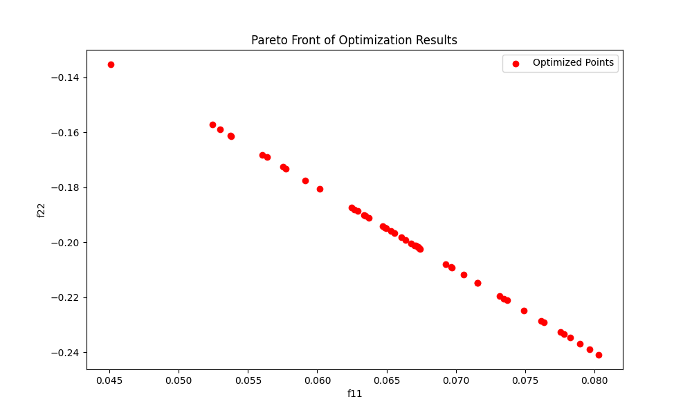
We select the $\ell_{1}$ penalized regression problem and the exact penalty model as the objective functions to construct a nonsmooth multiobjective problem as follow:

$$\min_{\bf{0}\leq x\leq\bf{1}} \left\|\max\{Ax,0\}-b\right\|_{1}+0.01\left\|x\right\|_{1}$$ (45)

$$\min_{\bf{-1}\leq x\leq\bf{1}} -\max\{\left\|Ax-b\right\|_{1}-\hat{\epsilon},0\}-0.03\left\|x\right\|_{1},$$

For a given group of (m,n,Spar),the data in this example is generated as follow:

A = np.random.randn(100,200);  s = Spar * 200;  x = np.random.uniform(0,1,(200,1));  x[:200 - int(s)] = 0;  np.random.shuffle(x);  $x[x>1]=1$; bb = A.dot(x); b = np.maximum(bb, np.zeros(bb.shape)).

Set $\sigma=0.75,\alpha=4,\mu_{0}=0.5,\hat{\epsilon}=0.001$.We use the smoothing function defined in definition(2) for the objective functions.We randomly choose 50 initial points for the experiment,and the Pareto front of the results was drawn in the Figure.1.

Figure 1: the Pareto front of the $\ell_{1}$ penalized regression problem and the exact penalty model

Example 2

In numerical experiments, we have used single-objective convex test problems CB3, DEM, QL,LQ, Mifflin1 and Wolfe described in lukvsan2000test and combined these functions in order to obtain 11 multiobjective problems. The combinations used are described in Table 1. All our test problems are nonsmooth and convex. The dimension of all the test problems is two.

Table 1: Test problems

Problem	Objectives	Initial point
1	CB3&DEM	(2,2)
2	CB3&LQ	(2,2)
3	CB3&Mifflin1	(2,2)
4	CB3&Wolfe	(2,2)
5	DEM&QL	(2,4)
6	DEM&LQ	(1,1)
7	QL&LQ	(2,4)
8	QL&Mifflin1	(2,4)
9	QL&Wolfe	(2,2)
10	LQ&Mifflin1	(-0.5,-0.5)
11	LQ&Wolfe	(-2,-2)

We have used the implementation of MPB described in makela2003multiobjective where the two-point line search algorithm makela1992nonsmooth is employed,and MSGDB described in montonen2018multiple which is based on Armijo type rule armijo1966minimization due to its simplicity.The results of these two methods are from paper 2. We compare the results obtained by SAPGM algorithm on the same test problem with them, and draw the comparison results in Table 2 and Table 3.

Table 2: Results of numerical tests

Problem	SAPGM	Iteration	MSGDB	Iteration
1	(2.00000002,6.00000003)	1	(2.00280000,6.00960000)	8
2	(2.13229985,-1.06297233)	2	(2.00670000,-1.00330000)	7
3	(2.01978289,18.61116085)	2	(2.00710000,18.85670000)	7
4	(2.00625527,24.95787791)	2	(2.00900000,24.91500000)	8
5	(14.22223503,8.88889254)	2	(16.72460000,7.20190000)	5
6	(3.03469534,-1.00359315)	2	(4.24270000,-1.41420000)	3
7	(7.20687088,2.59835124)	2	(7.20390000,2.57610000)	7
8	(7.20000194,122.79998782)	3	(7.20010000,122.79550000)	3
9	(11.1836738,46.42857107)	2	(12.36690000,47.95620000)	2
10	(-0.50697636,-0.76882743)	5	(-1.01150000,-0.99980000)	6
11	(0.06689207,1.07027301)	2	(1.02140000,-7.44960000)	13
average		2.27		6.27

Table 3: Results of numerical tests

Problem	SAPGM	Iteration	MPB	Iteration
1	(2.00000002,6.00000003)	1	(3.56010000,3.78250000)	7
2	(2.13229985,-1.06297233)	2	(4.38790000,17.84860000)	12
3	(2.01978289,18.61116085)	2	(2.05030000,18.01510000)	17
4	(2.00625527,24.95787791)	2	(2.00650000,24.90590000)	8
5	(14.22223503,8.88889254)	2	(16.80000000,7.20000000)	7
6	(3.03469534,-1.00359315)	2	(4.11560000,-1.41290000)	5
7	(7.20687088,2.59835124)	2	(7.39080000,2.51450000)	6
8	(7.20000194,122.79998782)	3	(11.18260000,99.14890000)	12
9	(11.1836738,46.42857107)	2	(7.40910000,48.78910000)	11
10	(-0.50697636,-0.76882743)	5	(-1.06820000,-0.99750000)	13
11	(0.06689207,1.07027301)	2	(-1.03920000,12.47060000)	19
average		2.27		10.64

Let us take a closer look at the test problem number 2. In that problem, the objective functions are combined from test problems CB3 and LQ lukvsan2000test . Thus, objective functions of the problem (17) are now:

$$f_{1}(x) =\max\{x_{1}^{4}+x_{2}^{2},(2-x_{1})^{2}+(2-x_{2})^{2},2e^{x_{2}-x_{1}}\}$$ (46)

$$f_{2}(x) =\max\{-x_{1}-x_{2},-x_{1}-x_{2}+x_{1}^{2}+x_{2}^{2}-1\}.$$

The starting point is chosen to be $x_{0}=(2,2)^{T}$. The performance of MSGDB is described in Table 4 where current points and the function values at those points are listed at every iteration. As we see, the value of both objective functions decreases at every iterations.

Table 4: The performance of the SAPGM algorithm with test problem 2

Iteration	$x$	$f(x)$
0	(2,2)	(20.00000000,3.00000000)
1	(0.96745704,0.96745704)	(2.13228991,-1.06296782)
2	(0.96745519,0.96745408)	(2.13229985,-1.06297233)

Figure 2: The solutions obtained in objective space for test problem 2 with 10 random starting points.

In Fig.2,we show the Pareto front of the test problem 2,From Fig.2, we can observe that the solution obtained is quite sensitive for the selection of the starting point. With different starting points we can generate different (weakly) Pareto optimal solutions and obtain an approximation of the Pareto optimal set.

From results in Table 2 and Table 3, we can conclude that the number of iterations are approximately the same order, since according to the results, the average iterations needed for SAPGM is 2.27 and for MSGDB is 6.27 and for MPB is 10.64.Additionally, we observe that the methods produce mainly different weakly Pareto optimal solutions since the median relative distance of solutions in the objective space is 1.1409 varying in the interval from 0.0003 to 89.1013. This aspect is important, since instead finding only one solution efficiently, we are often interested to find several different weakly Pareto optimal solutions to approximate the Pareto frontier.

In the aforementioned test scenarios, it is noted that despite SAPGM requiring significantly fewer iterations than both MPB and MSGDB, the solutions obtained in a minority of cases did not exhibit a substantial superiority over those generated by MSGDB. Furthermore, it is observed that the iteration count of SAPGM is highly sensitive to the selection of parameters, specifically alpha and the ratio l/mu. Manual tuning of these parameters is imperative for achieving optimal outcomes in practical applications.

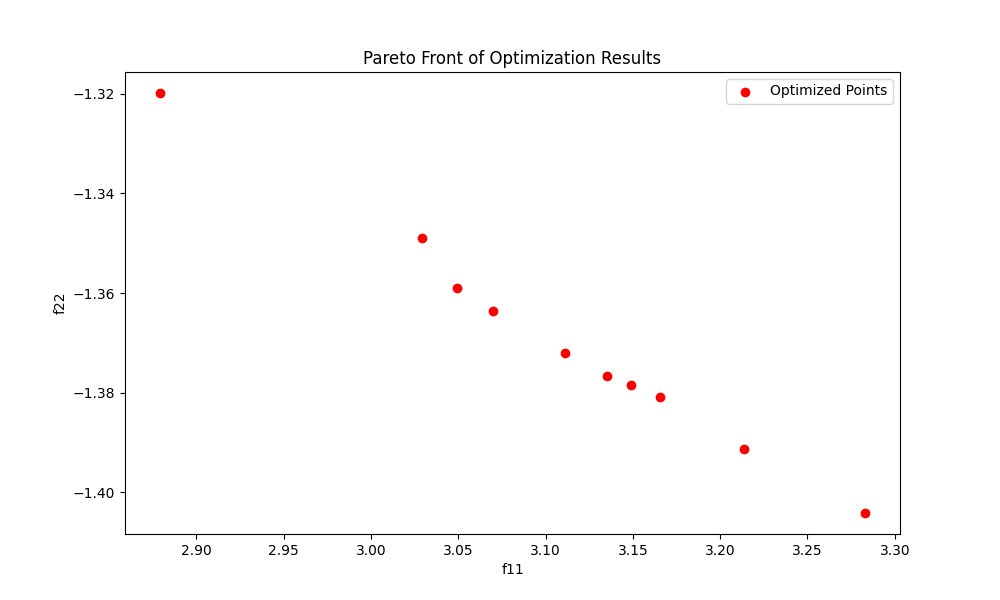
Example 3

For the universality assessment of the algorithmic results, we formulated a second-order test problem in the form of $f+g$.The test problem in the form of $f+g$ is as follow:

$$\min_{x} 200\max(|x_{1}|-x_{2},0)+0.5|x_{1}-1|$$ (47)

$$\min_{x} x_{1}^{4}+x_{2}^{2}+0.3\left\|x\right\|_{1}$$

Subsequently, we conducted testing and depicted its Pareto front in Fig.3.It can be seen from the image that the algorithm is still effective for second-order test problems, indicating that the algorithm has a wide range of application, and is not limited to first-order test problems.

Figure 3: The solutions obtained in objective space for second-order test problem with 10 random starting points.

7 Conclusions

In conclusion, this paper introduces a novel and efficient Smoothing Accelerated Proximal Gradient (SAPG) algorithm designed for the resolution of nonsmooth convex multiobjective optimization problems, as formulated in equation (1), where the objective function is the summation of two continuous convex functions. Emphasis is placed on the crucial role of the update method for the smoothing parameter in determining the convergence properties of the proposed algorithm. Each iteration involves employing the accelerated proximal gradient with an extrapolation coefficient of $\frac{k-1}{k+\alpha-1}$ to minimize the problem (1) with a fixed smoothing parameter, followed by an update to the smoothing parameter. The paper establishes that our proposed method achieves an enhanced convergence rate, improving from $O(1/k^{2})$ to $o(1/k^{2})$. Additionally, theoretical proofs affirm that the iterates sequence converges to an optimal solution of the problem. An effective strategy for solving the subproblem is presented through its dual representation. The results of numerical experiments underscore the superior performance of the SAPG algorithm and underscore the importance of extrapolation in achieving faster convergence rates.