Quantum Kernels for Symbolic Sequences Classification

Quantum Time Series Similarity Measures and Quantum Temporal Kernels

Abstract

This article presents a quantum computing approach to the design of similarity measures and kernels for classification of stochastic symbol time series. The similarity is estimated through a quantum generative model of the time series. We consider classification tasks where the class of each sequence depends on its future evolution. In this case a stochastic generative model provides natural notions of equivalence and distance between the sequences. The kernel functions are derived from the generative model, exploiting its information about the sequences evolution.We assume that the stochastic process generating the sequences is Markovian and model it by a Quantum Hidden Markov Model (QHMM). The model defines the generation of each sequence through a path of mixed quantum states in its Hilbert space. The observed symbols are emitted by application of measurement operators at each state. The generative model defines the feature space for the kernel. The kernel maps each sequence to the final state of its generation path. The Markovian assumption about the process and the fact that the quantum operations are contractive, guarantee that the similarity of the states implies (probabilistic) similarity of the distributions defined by the states and the processes originating from these states. This is the heuristic we use in order to propose this class of kernels for classification of sequences, based on their future behavior. The proposed approach is applied for classification of high frequency symbolic time series in the financial industry.

1 Introduction

Many machine learning algorithms for time series use various measures of similarity between examples to solve a wide range of problems, including classification, regression, density estimation, and clustering. The measures of similarity are critical part of the k-NN algorithms, feature-based algorithms, and kernel methods. Different similarity measures are intended to account for different types of similarity of the time series. One group of similarities are estimated directly in the original time series space. When the exact timing and synchronization of the data points are crucial the time series are compared synchronously, in lock-step, using an one-to-one alignment of the corresponding data points. Some common lock-step time series similarity measures include Euclidean Distance, Linear Time Warping (LTW)[1], Pearson Correlation Coefficient [2], Spearman Rank Correlation [3]. The synchronous methods are not applicable for series with different length and are unable to capture the local dependencies among adjacent positions within time series data. These problems can be resolved by using non-linear mappings between the time series which allow comparison of one to many points. This approach provides some degree of flexibility or ”warping” when aligning two time series. This flexibility makes it possible to find the optimal alignment between time series that may have variations in timing, speed, or phase. Examples of elastic similarity measures are the Longest Common Sub-sequence (LCSS) [4], Dynamic Time Warping (DTW) [5], Edit Distance [6], Move-Split-Merge (MSM) Distance [7], Piecewise Linear Approximation (PLA) Distance [8], Symbolic Aggregate Approximation (SAX) Distance [9], Elastic Ensemble Distance (EED) [10]. The synchronous and elastic similarities are estimated over the full time series and they are referred to as ”global similarities”. Other approaches measure the similarity with respect to local but representative patterns or ”shapelets” [11] within time series. For each time series, the similarity between the time series and each shapelet is calculated, and these values become distance features. Distance features can be defined by the global similarities measures as well. Any similarity measure creates a space - ”dissimilarity” feature spaces - where each time series is represented by its distance vector to the other time series.

Another group of very successful, similarity based methods - the kernel methods [12] - use a function which maps pairs of input series to the dot product of corresponding vectors in a high dimensional Hilbert space. The classical kernel functions calculate the dot product directly in the input space, without explicitly construction of vectors in the Hilbert space. If these functions are properly designed their outputs are measure of similarity between the input time series and between their high dimensional representations as well. The intention of the method is the high dimensional representations of the inputs to be linearly separated in the Hilbert space with respect to their class labels [13]. The kernel functions are possible due to the properties of the inner product structure within the Hilbert space [14]. Mercer’s theorem defines the necessary and sufficient conditions for a function to be a valid kernel function [13]. The kernel functions allow construction of linear discriminative algorithms for learning domains with non-linear decision boundaries. Examples of such algorithms are Support Vector Machines [15], Kernel Logistic and Ridge Regression [16], Kernel Discriminant Analysis [17], and many others. Kernel methods are used in unsupervised learning algorithms as well to capture non-linear structures in data: Kernel Principal Component Analysis [18, 19, 20], Non-linear Independent Component Analysis [21, 22], Kernel K-Means Clustering [23], Kernel Spectral Clustering [24], Kernel Density Estimation [25]. Numerous kernel functions have been introduced for input variables represented as fixed-length real vectors, including polynomial, inhomogeneous polynomial, Gaussian radial basis function, sigmoid kernel, and hyperbolic tangent kernels[12]. These kernels are not suitable in scenarios where the input variables consist of time series data with varying lengths. One simple solution to this problem is to align each vector to a common length. This can be accomplished by application of Linear Time Warping. A more sophisticated approach to the global alignment of sequences relies on optimized alignment and dynamic programming. The Dynamic Time Warping for example, optimally aligns two sequences by warping one to minimize dissimilarity between corresponding points. It computes local distances, constructs a distance matrix, and employs dynamic programming to find the optimal alignment, which is used to calculate the distance between the sequences. The distance is used to define the DTW kernel. If the goal is to estimate the significant local similarities then the method of local alignment score [26] could be used. The method uses dynamic programming and a scoring system to compute an optimal local alignment score, highlighting regions of strong similarity within the sequences. This score has been combined in [27] with a convolution kernel [28] to derive a local alignment kernel. For time series classification tasks with symbolic, noisy, or high dimensional data it is appropriate to use a kernel based on the Symbolic Aggregate Approximation (SAX) similarity measure [9].

The choice of a kernel type for particular machine learning task depends on the goal of the task and the specific characteristic of the process we are targeting. It would be valuable to have a systematic way to define the kernel class and parameters for a particular classification, regression or clustering task. Since a kernel function reflects an assumption about the metric relations between the time series, a possible approach is these metric relations to be defined from a probabilistic generative model which assigns likelihood to each time series. The underlying model’s distribution defines a feature space where the original data can be represented. The time series can be mapped to feature spaces of generation paths, likelihoods, likelihoods parameters, or likelihood gradients with respect to parameters. Generative model-based kernels provide a general way to measure similarity between data samples, especially when their underlying distribution is important. The method combines the power of generative models to capture data distributions with the flexibility of kernel methods for various machine learning tasks.

There are multiple ways for implementing of generative model-based kernels. The P-kernels [23, 29] estimate the similarity or distance between two time series based on the joint probability of their inference over common generation paths of states. These kernels assume the existence of a probabilistic generative model, such as a Hidden Markov Model or Gaussian Mixture Model, which defines the probability distribution of the sequences. This distribution serves as a reproducing kernel space. In this approach, each time series is transformed into a feature vector of probabilities over all possible inference paths— sequences of states or sets of mixture components. The similarity of two series is then computed by taking the dot product of their respective feature vectors, with each component weighted by the probability of the corresponding inference path. Due to the feature vector containing probabilities for all possible inference paths, these kernels are also known as marginalisation kernels. In another generative approach, known as probability product kernel [30], each time series is mapped to a distribution within a parameterized class of distributions. The probabilistic models for the individual time series are identified using maximum likelihood estimation. The probability product kernel is defined as standard inner product between densities. If the inner product in the product kernel is replaced by the Kullback-Leibler divergence of the densities, the resulting kernel is the Kullback-Leibler kernel [31].

Since the vectors in the feature space are probability distributions, the distance between them can be estimated using common divergence measures like the Kullback-Leibler divergence, Jensen-Shannon divergence, or other statistical distance measures [31, 32]

Another method for exploiting the knowledge captured by a probabilistic model to define a similarity metrics is to embed the time series in the gradient space of the generative model. This approach is known as Fisher Kernel [33]. The gradient vector of a series log-likelihood with respect to a model parameter describes how that parameter contributes to the generative process. These parameters can encompass transition and emission probabilities in the case of hidden Markov models, expectations, and variances in the context of Gaussian mixtures, and more. The gradient vector is known as Fisher score [34]. If two series have similar gradient vectors, it indicates the model generates them in a similar manner. Consequently, we consider the series being close to each other in terms of their generative processes. The Fisher kernel is defined as the inner product of the gradient vectors of any two time series.

In many discriminative learning tasks the class of a sequence depends on the distribution over its future evolutions. For example, the language models infer the most likely continuations of a sentence, the financial models estimate the probability a variable to be in a range in a future time, etc. In this article we study quantum models of discrete stochastic processes.

2 Preliminaries

2.1 Stochastic Process Languages

We consider a class of observable, discrete-time stationary stochastic processes denoted by

$$\{y_{t}:t\in\mathbb{N},y_{t}\in\Sigma\},$$ (1)

where $\Sigma=\{a_{1},\ldots,a_{m}\}$ is a finite set of symbols, called an alphabet.

The set of all finite sequences over the alphabet $\Sigma$, including the empty sequence $\epsilon$, is denoted by ${\Sigma}^{*}$. The set of all sequences with length exactly $t$ is denoted by ${\Sigma}^{t}$.

Any subset of ${\Sigma}^{*}$ is a language ${L}$ over the alphabet. The sequences belonging to a language are referred to as words.

The set of sequences originated by observations or measurements of the evolution of a discrete-time process is called the process language. It is easy to verify that if a word results from the observation of a process, then every one of its subwords has also been observed. Therefore, the process languages are subword-closed.

A stochastic process language $L$ is a process language together with a set

$$D^{L}=\bigl{\{}D_{t}^{L}:t\geq 0\bigr{\}}$$ (2)

of finite dimensional probability distributions $D_{t}^{L}$, each of which is defined on the sequences with length exactly $t$:

$$D_{t}^{L}=\bigl{\{}P[\textbf{y}]:\textbf{y}\in{\Sigma}^{t},\sum_{\textbf{y}\in{\Sigma}^{t}}P[\textbf{y}]=1\bigr{\}}$$ (3)

2.2 Probabilistic Generative Models

We will consider probabilistic generative models of stochastic process languages. These models assign probability to each sequence from $\Sigma^{*}$. Examples of such models are Variational Autoencoders (VAEs), Gaussian Mixture Models (GMMs), Hidden Markov Models (HMMs), Latent Dirichlet Allocation (LDA), Bayesian Networks, Boltzmann Machines, etc.

A generative model of stochastic language can be defined assuming that each observation $Y_{t}$ depends on the state of a non-observable or hidden finite-state process

$$\{x_{t}:t\in\mathbb{N},x_{t}\in S\},$$ (4)

where $S=\{s_{1}\ldots s_{n}\}$. The joint process

$$\{y_{t},x_{t}:t\in\mathbb{N},\,y_{t}\in{\Sigma},\,x_{t}\in S\}$$ (5)

is stationary and can be described by a linear model

$$\begin{array}[]{lcl}x_{t+1}=Ax_{t}\\ y_{t}=Bx_{t},\end{array}$$ (6)

where at any moment in time $t$, the model is in a superposition (stochastic mixture) of its hidden states, described by a stochastic vector $x_{t}\in\mathbb{R}^{n}$. The component $x_{t}^{i}$ represents the probability of being in state $x_{t}=s_{i}$. The distribution of observable symbols at time at time $t$ is defined by the stochastic vector $y_{t}\in\mathbb{R}^{m}$ as the probability to observe $y_{t}=a_{i}$ is $y_{t}^{i}$. This model is known as (classical) hidden Markov model (HMM).

For every HMM $\mathbf{M}$ we can define a set of observable operators T as

$$\textbf{T}=\{T_{a}:T_{a}=AB_{a},a\in\Sigma\}$$ (7)

where $B_{a}=\operatorname{diag}(B[a,i]),i\in 1..n$ are diagonal matrices defining symbol observation probabilities for each state $s_{i}$ [35, 36].

Every component $T_{a}[i,j]$ of an observable operator $T_{a}$ defines the conditional probability to observe symbol $a$ when the state process evolves from state $s_{i}$ to $s_{j}$.

$$T_{a}[i,j]=P[s_{j}\mid s_{i},a].$$

Let $\textbf{a}={a_{1}}\ldots{a_{t}}$ be any sequence. We define an observable operator corresponding to a as follows:

$$T_{\textbf{a}}=T_{a_{l}}\ldots T_{a_{1}}.$$

A Hidden Markov Model (HMM) $\mathbf{M}$ defines the probability of every finite observable sequence $\mathbf{a}=a_{1}\ldots a_{t}$ as:

$$P[\textbf{a}|\mathbf{M}]=\textbf{1}T_{a_{t}}\ldots T_{a_{1}}\textbf{x}_{0}=\textbf{1}T_{\textbf{a}}\textbf{x}_{0},$$ (8)

where 1 is the unit row vector with dimension $n$, and $\textbf{x}_{0}$ is an initial states distribution.

With every model $\mathbf{M}$ we associate a sequence function $f^{\mathbf{M}}:{\Sigma}^{*}\rightarrow\left[0,1\right]$ defined as:

$${f^{\mathbf{M}}}(\textbf{a})=P(\textbf{a}|\mathbf{M}),\forall\textbf{a}\in{\Sigma}^{*}.$$ (9)

Through the function $f^{\mathbf{M}}$ the model defines a stochastic process language $L_{M}$ (3):

$$D^{\mathbf{M}}_{t}=\{{f^{\mathbf{M}}}(\textbf{a}):\textbf{a}\in{\Sigma}^{t}\}$$ (10)

2.3 Classification Problem for Stochastic Languages

We consider symbolic sequences classification problem for a stochastic process language $L$ and a finite set of class labels $C=\bigl{\{}c_{1},\cdots,c_{k}\bigr{\}}$. It is assumed that there exists an unknown probabilistic classification map $\mathcal{P}:L\rightarrow P[C]$ assigning to each sequence $\mathbf{y}\in L$ a distribution over the class labels. A convenient way to define the classification map is to use a mapping function

$$p(\mathbf{y},c)=P[c|\mathbf{y}],\mathbf{y}\in L,c\in C$$ (11)

that estimates the probability of each class label $c$ for a given data instance $\mathbf{y}$.

A training data sample is defined as follows:

$$S=\bigl{\{}(\mathbf{y}_{i},c_{i}):\mathbf{y}_{i}\in Y,c_{i}\in C,i\in\left[1,l\right]\bigr{\}},$$

where $Y=\bigl{\{}\mathbf{y}_{i}:\mathbf{y}_{i}\sim D^{L}_{|\mathbf{y}_{i}|},i\in\left[1,l\right]\bigr{\}}$ is a set of finite length sequences sampled from the distributions $D^{L}$ of $L$.

The goal of the classification problem is to learn an approximation $\mathcal{\hat{P}}$ of the unknown probabilistic classification map.

The performance of the approximated mapping function $\hat{p}(\mathbf{y},c)$ is typically evaluated using probabilistic metrics such as log-likelihood, Brier score, or other probabilistic measures [???]. These metrics assess the model’s ability to predict the probability distribution over class labels and quantify the quality of the stochastic classification results.

2.4 Kernel Functions

A common approach to the solution of the classification problem is to define a similarity measure for pairs of sequences that is consistent with their classes: the sequences belonging to the same class to be closer according to this measure compared to sequences from different classes. A method to formalize the similarity measure is to define a kernel function from the original sequence space to a high dimensional feature space. The intention is the kernel function to linearize the relationships between input and output variables in the feature space. The kernel function approach is a standard which allows the expansion of conventional linear algorithms for classification, regression, and other learning tasks to effectively address nonlinear scenarios.

By contrast, a kernel-based discriminative approach like a support vector classifier starts by properly choosing a kernel, or equivalently a feature map $\phi:X\rightarrow F$, conceptually embeds the data in F and uses the training data to find a linear discriminant in the feature space. Of course, the overall performance will depend strongly on the choice of the kernel: this choice should reflect the prior knowledge about how the data was generated. Lately, there have been many approaches to automatically learn the kernel from data (for instance, [37]). But even in those there is always a prior step where at least a suitable family of kernels must be chosen. Generative kernels try to combine the advantages of both generative and discriminative approaches by introducing generative models on data and use them to devise a kernel. This can be done in many ways: (i) mapping data to points in a probability space and devising a kernel between probability distributions, (ii) considering a fixed probability distribution and study how does it “fit” each data point, (iii) assuming that there is some hidden model that governs the data generation and marginalizing with respect to this model, etc. W

Following the kernel construction approach, we map the input sequences $\mathbf{x}\in X$ to a high-dimensional quantum Hilbert space $H$. The purpose of this mapping, denoted as $\phi:X\rightarrow H$, is to make the output variables linearly separable with respect to their classes. We will use the quantum generator () to define a quantum kernel function $\kappa:X\times X\rightarrow\mathbb{R}$ to compute the inner product in $H$ without the need to explicitly construct its vectors:

$$\kappa(x_{1},x_{2})=\langle\phi(x_{1}),\phi(x_{2})\rangle$$

The existence of such functions $\kappa$, referred to as kernel functions, is a result of the properties of the inner product structure within a Hilbert space. Mercer’s theorem defines the necessary and sufficient conditions for a function to be a valid kernel function. The kernel functions allow construction of classification and regression learning algorithms that are nonlinear in the input space $X$ while having linear counterparts within the Hilbert space $H$.

2.5 Quantum Hidden Markov Models

We will consider stochastic process languages defined by quantized HMMs known as Quantum Hidden Markov Models (QHMMs) [38]. A QHMM is a complete positive quantum operation [39] or quantum channel, describing how a composite quantum system evolves according to its internal dynamics and simultaneously parts of it are observed by measurement. The model combines unitary hidden states evolution with the emission of observations correlated with the hidden states. The QHMM is a quantum stochastic generator, formally defined as follows:

Definition 1 (Quantum Hidden Markov Model [38]).

A quantum HMM (QHMM) $\mathbf{Q}$ over an $N$-dimensional Hilbert space $\mathcal{H}$ is a 4-tuple:

$$\mathbf{Q}=\{\Sigma,\,\mathcal{H},\,\mathcal{T}=\{T_{a}\}_{a\in\Sigma},\,\rho_{0}\},$$ (12)

where

• $\Sigma$ is a finite alphabet of observable symbols.

• $\mathcal{H}$ is an $N$-dimensional Hilbert space with space of density operators $D(\mathcal{H})$.

• $\mathcal{T}$ is a CPTP map (quantum channel) $\mathcal{T}:D(\mathcal{H})\rightarrow D(\mathcal{H})$.

• $\{T_{a}\}_{a\in\Sigma},\sum_{a\in\Sigma}T_{a}^{\dagger}T_{a}=I_{N}$ is an operator-sum representation of $\mathcal{T}$ in terms of a complete set of Kraus operators.

• $\rho_{0}$ is an initial state, $\rho_{0}\in D(\mathcal{H})$, where $D(\mathcal{H})$ is the space of density operators defined in $\mathcal{H}$.

When the operation $\mathcal{T}=\{T_{a}\}_{a\in\Sigma}$ is applied to a state $\rho\in D(\mathcal{H})$, the model $\mathbf{Q}$ defines measurement outcome $a\in\Sigma$ with probability:

$$P\bigl{[}a|\rho\bigr{]}=\operatorname{tr}(T_{a}\rho)$$ (13)

and the system’s state after the measurement becomes:

$$\rho_{a}=\frac{T_{a}\rho}{P\bigl{[}a|\rho\bigr{]}}.$$ (14)

The completeness of the set of Kraus operators $\{T_{a}\}_{a\in\Sigma}$ guarantees that the measurement probabilities in each state define a distribution:

$$D^{\mathbf{Q}}_{\rho}=\{P\bigl{[}a|\rho\bigr{]}:a\in\Sigma\}$$ (15)

If the operation $\mathcal{T}$ is applied $t$ times starting at the initial state a time series $\mathbf{a}=a_{1}\ldots a_{t}$ will be observed with probability

$$P\bigl{[}\mathbf{a}|\rho_{0}\bigr{]}=\operatorname{tr}(T_{\mathbf{a}}\rho_{0}).$$ (16)

and the final state will be

$$\rho_{\mathbf{a}}=\frac{T_{\mathbf{a}}\rho_{0}}{P\bigl{[}\mathbf{a}|\rho_{0}\bigr{]}}.$$ (17)

where

$$T_{\mathbf{a}}=T_{a_{t}}\ldots T_{a_{1}}$$

For each QHMM $\mathbf{Q}$ the equation (16) defines a sequence function $f^{\mathbf{Q}}$ as follows:

$$f^{\mathbf{Q}}(\mathbf{a})=P\bigl{[}\mathbf{a}|\rho_{0}\bigr{]},\forall\mathbf{a}\in\Sigma^{*},$$ (18)

The sequence function (18) defines a distribution $D^{\mathbf{Q}}_{t}$ over the sequences of length $t$ for $\forall t>0$, since the quantum operation $\mathcal{T}$ is completely positive:

$$D^{\mathbf{Q}}_{t}=\bigl{\{}{f^{\mathbf{Q}}}(\textbf{a}):\textbf{a}\in{\Sigma}^{t}\bigr{\}}$$ (19)

Therefore every QHMM $\mathbf{Q}$ defines a stochastic process language $L^{\mathbf{Q}}$ (2) over the set of finite sequences $\Sigma^{*}$.

The Definition 1 of a QHMM is based on the concept of a POVM operation acting on a quantum state. The emission of the observable symbols is encoded in the operational elements (Kraus operators) of the quantum operation. This framework provides a convenient way to view QHMMs as channels for quantum information processing. It allows for the analysis of their informational complexity, expressive capacity, and establishes connections to stochastic process languages and the corresponding automata. However, this approach cannot be directly used for implementation of the QHMMs on quantum computing hardware. A critical result in quantum information theory - the Stinespring’s representation theorem  [40] - provides approach to the physical implementation of quantum channels and correspondingly of QHMMs. According to the theorem any quantum channel can be realized as a unitary transformation on a larger system (the combined hidden state and observable systems) followed by a partial trace operation that discards the observable system. An immediate consequence of this result is the following definition of QHMMs in the unitary circuits model of computation:

Definition 2 (Unitary Quantum Hidden Markov Model).

A Unitary Quantum HMM $\mathbf{Q}$ over a finite alphabet of observable symbols $\Sigma$ and finite $N$-dimensional Hilbert space is a 6-tuple:

$$\mathbf{Q}=\bigl{\{}\Sigma,\mathcal{H}_{S},\mathcal{H}_{E},U,\mathcal{M},R_{0}\bigr{\}}$$

where

• $\Sigma$ is a finite set of $m$ observable symbols.

• $\mathcal{H}_{S}$ is the Hilbert space of the hidden state system of dimension $N$.

• $\mathcal{H}_{E}$ is the Hilbert space of an auxiliary emission system with dimension $m\leq M\leq N^{2}$ and orthonormal basis $E=\{\ket{e_{i}}\}^{M-1}_{i=0}$.

• $U$ is a unitary operator defined on the bipartite Hilbert space $\mathcal{H}_{S}\otimes\mathcal{H}_{E}$.

• $\mathcal{M}$ is a bijective map $\mathcal{P}_{m}^{E}\rightarrow\Sigma$, where $\mathcal{P}_{m}^{E}$ is an $m$-element partition of $E$.

• $R_{0}=\rho_{0}\otimes\ket{e_{0}}\bra{e_{0}}$ is an initial state.

The equivalence of the Definition 1 of a QHMM as quantum channel and the unitary representation Definition 2 is defined by the operator-sum representation [39] of the quantum operation $\mathcal{T}$ as follows:

$$\mathcal{T}\cdot=\sum_{e\in\{\ket{e_{i}}\}^{M-1}_{i=0}}T_{e}\cdot T_{e}^{\dagger}.$$ (20)

where the Kraus operators $\{T_{e}\}$ act on the hidden system states and are defined as follows:

$$T_{e}=\left(I^{N}\otimes\bra{e}\right)U\left(I^{N}\otimes\ket{e_{0}}\right).$$ (21)

The Kraus operators depend on the unitary $U$, and the arbitrary selected orthonormal basis $\{\ket{e}\}$ of the emission system.

3 Quantum Generative Kernels

In this section, we introduce measures of similarity for sequences sampled from a stochastic process language. We assume that a generative model of the language (12) is given and define the similarity through this model.

3.1 Predictive Generative Kernels

The first measure estimates the similarity by evaluating the stochastic distance between the expected future evolutions of the sequences. Since the evolution of a Markovian process depends only of its initial state, it is easy to verify that if two sequences $\mathbf{y}$ and $\mathbf{z}$ define the same quantum sate $\rho$ of the model:

$$\rho=\frac{T_{\mathbf{y}}\rho_{0}}{P\bigl{[}{\mathbf{y}|\rho_{0}\bigr{]}}}=\frac{T_{\mathbf{z}}\rho_{0}}{P\bigl{[}{\mathbf{z}|\rho_{0}\bigr{]}}},$$

then the sequences $\mathbf{y}$ and $\mathbf{z}$ are equivalent in sense, that they define the same future distributions of the observables.The following proposition generalizes this idea by proving that if two states are close in trace norm, the corresponding forward distributions of the sequences are close in total variation distance.

Proposition 1.

For any two states $\rho_{1}$ and $\rho_{2}$ of a QHMM $\mathbf{Q}$ the total variation distance of the observable distributions $P\bigl{[}\mathbf{a}|\rho_{1}\bigr{]}$ and $P\bigl{[}\mathbf{a}|\rho_{2}\bigr{]}$ for $\mathbf{a}\in\Sigma^{l},l>0$ is bounded by the trace distance between the states $\rho_{1}$ and $\rho_{2}$.

Proof.

The similarity between the quantum states $\rho_{1}$ and $\rho_{2}$ can be estimated by their trace distance:

$$\mathcal{D}(\rho_{1},\rho_{2})=\frac{1}{2}\text{tr}|\rho_{1}-\rho_{2}|,$$ (22)

where

$$|\rho_{i}|\equiv\sqrt{\rho_{i}^{\dagger}\rho_{i}},i=1,2$$

The probabilities the same sequence $\mathbf{a}\in\Sigma^{l}$ to be observed at states $\rho_{1}$ and $\rho_{2}$ respectively are (16)

$$P\bigl{[}\mathbf{a}|\rho_{1}\bigr{]}=\operatorname{tr}(T_{\mathbf{a}}\rho_{1})$$ (23)

and

$$P\bigl{[}\mathbf{a}|\rho_{2}\bigr{]}=\operatorname{tr}(T_{\mathbf{a}}\rho_{2})$$ (24)

The difference between these probabilities is defined as follows:

$$P\bigl{[}\mathbf{a}|\rho_{1}\bigr{]}-P\bigl{[}\mathbf{a}|\rho_{2}\bigr{]}=\operatorname{tr}(T_{\mathbf{a}}(\rho_{1}-\rho_{2}))$$ (25)

Since the operation $T_{a}$ is trace non-increasing we have:

$$P\bigl{[}\mathbf{a}|\rho_{1}\bigr{]}-P\bigl{[}\mathbf{a}|\rho_{2}\bigr{]}\leq\operatorname{tr}(\rho_{1}-\rho_{2}).$$ (26)

If we assume that $P\bigl{[}\mathbf{a}|\rho_{1}\bigr{]}\geq P\bigl{[}\mathbf{a}|\rho_{2}\bigr{]}$ then

$$\bigl{|}P\bigl{[}\mathbf{a}|\rho_{1}\bigr{]}-P\bigl{[}\mathbf{a}|\rho_{2}\bigr{]}\bigr{|}\leq 2\mathcal{D}(\rho_{1},\rho_{2}).$$ (27)

The total variation distance between the distributions $P_{1}(\mathbf{a})=P\bigl{[}\mathbf{a}|\rho_{1}\bigr{]}$ and $P_{2}(\mathbf{a})=P\bigl{[}\mathbf{a}|\rho_{2}\bigr{]}$ is

$$\delta(P_{1},P_{2})=\sup_{\mathbf{a}\in\Sigma^{l}}\bigl{|}P_{1}(\mathbf{a})-P_{2}(\mathbf{a})\bigr{|}$$ (28)

$$\delta(P_{1},P_{2})\leq 2\mathcal{D}(\rho_{1},\rho_{2})$$ (29)

∎

This proposition implies that when, at a specific time $t=t_{0}$, two hidden states of the model are close in trace norm, the distributions of the observable processes originated from these states will be close in total variation distance for $t>t_{0}$.

To understand the importance of this fact in the context of kernels for discriminative tasks, let’s consider a specific classification problem. In this problem, each observed sequence $\mathbf{y}\in L^{Q}$ is classified based on its $k$-step future evolution. More formally, if at time $t_{0}$ we have observed the sequence $\mathbf{y}$ and at time $t_{0}+k$ we have observed the sequence $\mathbf{ya}$, then the class of $\mathbf{y}$ depends only of some feature of the sequence $\mathbf{a}$. We assume that the class can be computed by a function $f:\Sigma^{k}\rightarrow C$. As the sequence $\mathbf{y}$ is sampled from the stochastic language $L^{Q}$ described by the generative model $Q$ (12), the mapping function (11) can be defined as follows :

$$p(\mathbf{y},c)=\sum_{\mathbf{a}\in\Sigma^{k}}P\bigl{[}\mathbf{a}|\mathbf{y}\bigr{]}\cdot I_{f({\mathbf{a})=c}},$$ (30)

where

$$P\bigl{[}\mathbf{a}|\mathbf{y}\bigr{]}=P\bigl{[}\mathbf{a}|\rho_{\mathbf{y}}\bigr{]},$$

and from (14)

$$\rho_{\mathbf{y}}=\frac{T_{\mathbf{y}}\rho_{0}}{P\bigl{[}{\mathbf{y}|\rho_{0}\bigr{]}}},$$

The mapping function (30) defines a distribution over the class labels:

$$CP_{\mathbf{y}}(c)=\bigl{\{}p(\mathbf{y},c):c\in C\bigr{\}}$$

Any other sequence $\mathbf{z}\in L^{Q}$ defines distribution $CP_{\mathbf{z}}$ at total variation distance w.r.t $CP_{\mathbf{y}}$:

$$\delta(CP_{\mathbf{y}},CP_{\mathbf{z}})=\sup_{c\in C}\bigl{|}CP_{\mathbf{y}}(c)-CP_{\mathbf{z}}(c)\bigr{|}$$ (31)

$$\delta(CP_{\mathbf{y}},CP_{\mathbf{z}})=\sup_{c\in C}\sum_{\mathbf{a}\in\Sigma^{k}}\bigl{|}P\bigl{[}\mathbf{a}|\mathbf{y}\bigr{]}-P\bigl{[}\mathbf{a}|\mathbf{z}\bigr{]}\bigr{|}\cdot I_{f({\mathbf{a})=c}}$$ (32)

From Proposition 1:

$$\delta(CP_{\mathbf{y}},CP_{\mathbf{z}})\leq 2\mathcal{D}(\rho_{\mathbf{y}},\rho_{\mathbf{z}})\cdot\sup_{c\in C}\sum_{\mathbf{a}\in\Sigma^{k}}I_{f({\mathbf{a})=c}}$$ (33)

$$\delta(CP_{\mathbf{y}},CP_{\mathbf{z}})\leq C\cdot\mathcal{D}(\rho_{\mathbf{y}},\rho_{\mathbf{z}}),$$ (34)

where

$$C=2\sup_{c\in C}\sum_{\mathbf{a}\in\Sigma^{k}}I_{f(\mathbf{a})=c}$$

is a constant depending on the structure of the classification task.

This result demonstrates that the variation distance between the classification distributions of two sequences is bounded by the trace distance between the corresponding quantum states. This motivates us to define the similarity between every pair of time series $\mathbf{t}_{1}$ and $\mathbf{t}_{2}$ by mapping them to the quantum states $\rho_{1}$ and $\rho_{2}$ of the model (1), and calculating the trace distance between these states. It is important to emphasize that this measure of similarity pertains to the future evolution of the time series. We define the predictive generative kernel as follows:

$$\kappa(\mathbf{y},\mathbf{z})=\mathcal{D}\bigl{(}\phi(\mathbf{y}),\phi(\mathbf{z})\bigr{)},\mathbf{y},\mathbf{z}\in L^{Q}$$ (35)

where the mapping $\phi(\mathbf{y})$ of a sequence $\mathbf{y}$ to quantum state $\rho_{\mathbf{y}}$ is defined as:

$$\phi(\mathbf{y})=\frac{T_{\mathbf{y}}\rho_{0}}{P\bigl{[}{\mathbf{y}|\rho_{0}\bigr{]}}},\mathbf{y}\in L^{Q},$$

and $\mathcal{D}(\rho_{\mathbf{y}},\rho_{\mathbf{z}})$ is the trace distance of the quantum states (22). Since the trace distance is a symmetric, positive semi-definite function the equation (35) defines a valid kernel.

Another predictive quantum kernel can be defined by the Bures metric between two quantum states defined as

$$\mathcal{B}(\rho_{\mathbf{y}},\rho_{\mathbf{z}})=2-2\sqrt{F(\rho_{\mathbf{y}},\rho_{\mathbf{z}})},$$

where the quantum fidelity $F(\rho_{\mathbf{y}},\rho_{\mathbf{z}})$ is defined as:

$$F(\rho_{\mathbf{y}},\rho_{\mathbf{z}})=\left(\text{Tr}\left(\sqrt{\sqrt{\rho_{\mathbf{y}}}\rho_{\mathbf{z}}\sqrt{\rho_{\mathbf{y}}}}\right)\right)^{2}.$$

Since the Bures metric is symmetric and positive semi-definite it defines a valid kernel:

$$\kappa(\mathbf{y},\mathbf{z})=\mathcal{B}\bigl{(}\phi(\mathbf{y}),\phi(\mathbf{z})\bigr{)},\mathbf{y},\mathbf{z}\in L^{Q}.$$ (36)

3.2 Structural Generative Kernels

The key idea is these kernels to estimate the similarity between time series by matching of their substructures. The structure of each time series is defined by the evolution of its hidden quantum state. Therefore it is reasonable to estimate the structural similarity by the divergence of appropriate statistics of their generative processes. The other intuition supporting the idea to compare the generative statistics is that the observable sequences depend on causal latent factors, represented by the hidden states. We can assume that the semantics of each sequence is defined by the level of participation of each of the hidden states. Therefore the structural similarity can be measured by the divergence of the expectations of the hidden states.

To formalize these ideas, let’s consider the process of generation of a sequence $\mathbf{y}\in L^{Q},\mathbf{y}=y_{1}y_{2}\cdots y_{n},y_{i}\in\Sigma,i\in[1,n]$. Initially the model is in state $\rho_{0}$. After the generation of the first symbol $y_{1}$ the system is state $\rho_{1}$ defined as follows:

$$\rho_{1}=\frac{T_{y_{1}}\rho_{0}}{tr(T_{y_{1}}\rho_{0})}$$

The state after the generation of the second symbol $y_{2}$ is defined as:

$$\rho_{2}=\frac{T_{y_{2}}\rho_{1}}{tr(T_{y_{2}}\rho_{1})}$$

Finally, the end state is

$$\rho_{n}=\frac{T_{y_{n}}\rho_{n-1}}{tr(T_{y_{n}}\rho_{n-1})}$$

We propose to map the sequence of symbols $\mathbf{y}=y_{1}y_{2}\cdots y_{n}$ to the expected state of the its generative sequence of states $\rho_{1}\rho_{2}\cdots\rho_{n}$ as follows:

$$\phi_{s}(\mathbf{y})=\hat{\rho}_{\mathbf{y}}=\frac{1}{n}\sum_{i\in[1,n]}\rho_{i}$$

It is easy to demonstrate, that the average of a set of density matrices is a density matrix. Therefore, the expectation $\hat{\rho}$ is a quantum state and we can define a valid structural quantum kernel using the trace distance as follows:

$$\kappa_{s}(\mathbf{y},\mathbf{z})=\mathcal{D}\bigl{(}\phi_{s}(\mathbf{y}),\phi_{s}(\mathbf{z})\bigr{)},\mathbf{y},\mathbf{z}\in L^{Q}$$ (37)

A valid structural kernel can be defined using Bures metric as well:

$$\kappa_{s}(\mathbf{y},\mathbf{z})=\mathcal{B}\bigl{(}\phi_{s}(\mathbf{y}),\phi_{s}(\mathbf{z})\bigr{)},\mathbf{y},\mathbf{z}\in L^{Q}$$ (38)

4 Quantum Kernels in Quantum Circuits Computing Model

For each sequence $\textbf{a}\in{\Sigma}^{*}$ a quantum generative model $Q$ (12) defines a probability $P\bigl{[}\textbf{a}|G\bigr{]}$, and hence $G$ defines distribution on all continuations $\textbf{b},|\textbf{b}|=t$ of the sequence:

$$D_{t}^{\textbf{a}}=\bigl{\{}P\bigl{[}\textbf{b}|\textbf{a},G\bigr{]}=P\bigl{[}\textbf{a}\textbf{b}|G\bigr{]}:\textbf{b}\in\Sigma^{t}\bigr{\}}$$

In many cases the class of a sequence depends on the current state and the probability of its continuations. For example, in a financial time series of price movements the class of a sequence can be 1 if the next movement is expected to be ”UP”. In an English sentence the class of a phrase is ”subject” if the expected next word is a verb. In these cases we classify the sequence by the distributions of their continuations. Therefore it is natural to assume that if the induced future distributions of two sequences are close, the similarity of these sequences is high. Let’s formalize this intuitive explanation. Let $\mathbf{a}=a_{1}\ldots a_{k}$ and $\mathbf{b}=b_{1}\ldots b_{l}$ are the sequences we want to compare. The model $Q$ defines the following end states for each of them:

$$\rho_{\mathbf{a}}=T_{a_{k}}\ldots T_{a_{1}}\rho_{0}$$

$$\rho_{\mathbf{b}}=T_{b_{l}}\ldots T_{b_{1}}\rho_{0}$$

.

The use of quantum computing for non-linear mapping into a higher-dimensional vector space for non-linear classification was discussed for almost a decade in different sources, e.g. [41, 42, 43, 44, 45].

In the field of quantum machine learning a quantum kernel is often defined as the inner product between two data-encoding feature vectors $\rho_{\mathbf{a}}$, $\rho_{\mathbf{b}}$ [46]:

$$k_{1,2}=Tr\{\rho_{\mathbf{a}}\rho_{\mathbf{b}}\}$$

This definition works well, when feature maps are implemented by unitary operations on quantum circuits. In quantum computing there is a vital need to verify and characterize quantum states, where the fidelity is an important and useful similarity measure. There are a number of proposals for estimating the mixed state fidelity on a quantum computer, which overcome hardness limitations of classical algorithms. One proposal is a variational quantum algorithm for low-rank fidelity estimation [47]. Another proposal with exponential speedup [48] relies on state purifications being supplied by an oracle. Other variational algorithms have been proposed for the fidelity and trace distance [49]. A number of quantum measures of distinguishability are discussed in [50]. Special consideration should be given to working with mixed states. Classical fidelity measure was introduced by Richard Jozsa [51]. [52] gives most recent review of mixed states fidelity measures.

In the case of more general feature maps producing mixed states we define a kernel function $\kappa$ as follows:

$$\kappa(\mathbf{a},\mathbf{b})=1-\mathcal{D}(\rho_{\mathbf{a}},\rho_{\mathbf{b}}),$$

where $\mathcal{D}$ is a distance between two general quantum states, represented by their density matrices.

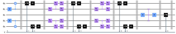
Figure 1: Implementation of SWAP test for market QHMM

X basis $\ket{\psi}$ & [wires=1]H

Y basis $\ket{\psi}$ & [wires=1]S^† [wires=1]H

Z basis $\ket{\psi}$ &

Figure 2: Measurements of the single qubit state in X, Y and Z bases

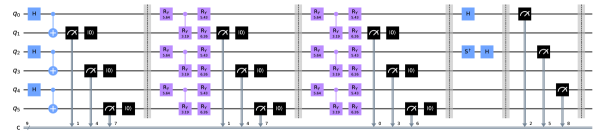
Figure 3: Implementation of projective kernel for market QHMM circuit

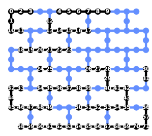
Figure 4: Initial qubit layout on ibm_nazca device for projected kernel approach

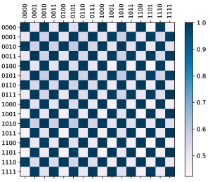
Figure 5: Color bar plot of the kernel matrix estimated on (ibm_nazca) device using projected kernels approach

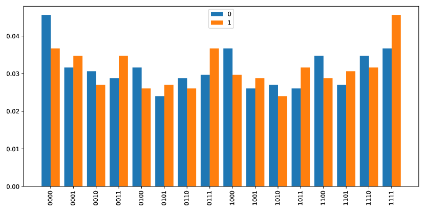
Figure 6: Next Symbol Distributions for $4$-symbol Sequences

5 Examples: The Limit Order Book

5.1 Artificial market example with four hidden states

In our previous paper [53] we have discussed the artificial $4$ states market example with binary observable, where the distribution of sequences was defined through classical hidden Markov model with defined state transitions and symbol emissions probability matrices. We showed that $\mathcal{H}_{S}$ (state system) and $\mathcal{H}_{E}$ (emission) are Hilbert spaces with dimension $2$, so the combined space $\mathcal{H}_{E}\otimes\mathcal{H}_{S}$ circuit required only two qubits. QHMM defining market distribution was trained with evolutionary algorithm.

In this section we will construct a kernel matrix for all pairs of sequences. One possible approach to implement this on the hardware is to use SWAP test [54] as shown on FIG 1. Qubits $q_{0}$, $q_{1}$ and $q_{3}$, $q_{4}$ on FIG 1 implement two QHMMs, $q_{2}$ is used for fidelity calculation. Maximally mixed states are prepared for both QHMMs leveraging classical registers $1$ and $3$. Then the circuit implements two steps of QHMM generator. Classical registers $1$ and $0$ capture the symbols of the first sequence, registers $3$ and $2$ of the second. Finally, the probability of measuring $0$ on qubit $q_{2}$ captured on classical register $4$ can be converted to the squared fidelity [54] as

$$|\langle{\phi}|\psi\rangle|^{2}=2\times(-0.5+\#\{(0)\}_{q_{2}}\times R^{-1})$$

where $\phi$ and $\psi$ are statevectors of respective state systems of both QHMMs, $\#\{(0)\}_{q_{2}}$ is the number of observed $(0)$ on qubit $q_{2}$ and $R$ is the number of shots. The number of shots required is usually estimated as $O(n)$, where $n$ is the number of states. In our case, $n=2^{2t+1}$, where $t$ is the length of the sequence. Unfortunately, for sequences of length 7-8 this requires about 1 million shots or more. Another downside is that this approach assumes calculating kernel element for pure states. In general, we can be working with mixed states. A better approach is to use projective kernels [55]. It is well-known [39, 56] that a density matrix of a single qubit can be written as

$$\rho=\frac{1}{2}\left[1+\sum_{k}{r_{k}\sigma_{k}}\right]$$

where $\sigma_{k}$ are the Pauli matrices and $r_{k}$ is a real, three component vector. $\rho$ can be reconstructed from the three measurements results

$$r_{k}=\left\langle\sigma_{k}\right\rangle=tr(\rho\sigma_{k})$$

.

The circuit implementation [56] is shown on FIG 2. We can implement projective kernel for the market QHMM circuit as shown on FIG 3. Finally, the kernel element is constructed from two density matrices as $k_{1,2}=e^{-\gamma\lVert\rho_{1}-\rho_{2}\rVert^{2}}$, where $\lVert\rVert$ is a Frobenius norm and $\gamma$ is a hyperparameter (for now, we set $\gamma=1$). In order to boost the effective number of shots we propose to run multiple circuits simultaneously in parallel on a single chip by combining them on a single circuit (multi-programming [57, 58, 59]). With this in mind, the initial qubit layout on IBM Nazca device is shown on FIG 4, where we effectively use $72$ qubits. Color bar plot of the kernel matrix is shown on FIG 5. We see a perfect separation between classes. In this case the main system required only $1$ qubit. In case, we have systems of many qubits we can use 1-reduced density matrix (1-RDM) or N-RDM approximations.

The checkerboard pattern is not surprising. Let’s plot $5$-symbol sequences on a histogram and split counts for the fifth symbol between two bars, one for $0$ and one for $1$ (see FIG 6). This way we can see, which is the most likely suffix for $4$-symbol prefix. $0$ and $1$ alternate as we go from $0000$ to $1111$.

6 Conclusions and Outlook

Discussed quantum computing approach to the design of similarity measures and kernels for classification of stochastic symbol time series. Similarity of the states implies (probabilistic) similarity of the distributions defined by the states and the processes originating from these states. This is the heuristic we use in order to propose this class of kernels for classification of sequences, based on their future behavior. The proposed approach can be applied for classification of high frequency symbolic time series in the financial industry. We have shown two different approaches to calculating temporal quantum kernels on quantum computers and suggested multi-programming approach to increase utilization of quantum resources. We have shown that our approach leads to good separation between classes.

7 Acknowledgements

The authors thank Amol Deshmukh for fruitful discussions about this work.

The views expressed in this article are those of the authors and do not represent the views of Wells Fargo. This article is for informational purposes only. Nothing contained in this article should be construed as investment advice. Wells Fargo makes no express or implied warranties and expressly disclaims all legal, tax, and accounting implications related to this article.

References

- [1] H. Shimodaira, K.-i. Noma, M. Nakai, and S. Sagayama, “Dynamic time-alignment kernel in support vector machine,” in Advances in Neural Information Processing Systems (T. Dietterich, S. Becker, and Z. Ghahramani, eds.), vol. 14, MIT Press, 2001.
- [2] Y. Zheng, Q. Liu, E. Chen, Y. Ge, and J. L. Zhao, “Time series classification using multi-channels deep convolutional neural networks,” in Web-Age Information Management (F. Li, G. Li, S.-w. Hwang, B. Yao, and Z. Zhang, eds.), (Cham), pp. 298–310, Springer International Publishing, 2014.
- [3] J. Ye, C. Xiao, R. M. Esteves, and C. Rong, “Time series similarity evaluation based on spearman’s correlation coefficients and distance measures,” in Cloud Computing and Big Data (W. Qiang, X. Zheng, and C.-H. Hsu, eds.), (Cham), pp. 319–331, Springer International Publishing, 2015.
- [4] S. Aghabozorgi, A. Seyed Shirkhorshidi, and T. Ying Wah, “Time-series clustering – a decade review,” Information Systems, vol. 53, pp. 16–38, 2015.
- [5] H. Shimodaira, K.-i. Noma, M. Nakai, and S. Sagayama, “Dynamic time-alignment kernel in support vector machine,” in Advances in Neural Information Processing Systems (T. Dietterich, S. Becker, and Z. Ghahramani, eds.), vol. 14, MIT Press, 2001.
- [6] L. Chen and R. Ng, “- on the marriage of lp-norms and edit distance,” in Proceedings 2004 VLDB Conference (M. A. Nascimento, M. T. Özsu, D. Kossmann, R. J. Miller, J. A. Blakeley, and B. Schiefer, eds.), pp. 792–803, St Louis: Morgan Kaufmann, 2004.
- [7] A. Stefan, V. Athitsos, and G. Das, “The move-split-merge metric for time series,” IEEE Transactions on Knowledge and Data Engineering, vol. 25, no. 6, pp. 1425–1438, 2013.
- [8] H. Li, C. Guo, and W. Qiu, “Similarity measure based on piecewise linear approximation and derivative dynamic time warping for time series mining,” Expert Systems with Applications, vol. 38, no. 12, pp. 14732–14743, 2011.
- [9] J. Lin, E. Keogh, S. Lonardi, and B. Chiu, “A symbolic representation of time series, with implications for streaming algorithms,” in Proceedings of the 8th ACM SIGMOD Workshop on Research Issues in Data Mining and Knowledge Discovery, DMKD ’03, pp. 2–11, 06 2003.
- [10] J. Lines and A. Bagnall, “Time series classification with ensembles of elastic distance measures,” Data Mining and Knowledge Discovery, vol. 29, pp. 565–592, 2015.
- [11] L. Ye and E. Keogh, “Time series shapelets: a novel technique that allows accurate, interpretable and fast classification,” Data Mining and Knowledge Discovery, vol. 22, pp. 149–182, 2011.
- [12] B. Schölkopf and A. J. Smola, Learning with Kernels: Support Vector Machines, Regularization, Optimization, and Beyond. MIT press Cambridge, 2001.
- [13] V. N. Vapnik, Statistical Learning Theory. John Wiley & Sons, Inc, 1998.
- [14] C. Cortes and V. N. Vapnik, “Support-vector networks,” Machine Learning, vol. 20, pp. 273–297, 1995.
- [15] B. Boser, I. Guyon, and V. Vapnik, “A training algorithm for optimal margin classifiers,” in Proceedings of the Fifth Annual Workshop on Computational Learning Theory, (Pittsburgh), 1992.
- [16] K. P. Murphy, Machine Learning: A Probabilistic Perspective. The MIT Press, 2012.
- [17] E. Pȩkalska and B. Haasdonk, “Kernel discriminant analysis for positive definite and indefinite kernels,” IEEE Transactions on Pattern Analysis and Machine Intelligence, vol. 31, no. 6, pp. 1017–1032, 2009.
- [18] B. Schölkopf, A. Smola, and K. Müller, “Nonlinear component analysis as a kernel eigen-value problem,” Neural Computation, vol. 10, no. 5, pp. 1299–1319, 1998.
- [19] A. Pandey, H. De Meulemeester, B. De Moor, and J. A. Suykens, “Multi-view kernel pca for time series forecasting,” Neurocomputing, vol. 554, p. 126639, 2023.
- [20] B. Schölkopf, S. Mika, C. J. C. Burges, P. Knirsch, K. R. Müller, G. Raetsch, and A. Smola, “Input space vs. feature space in kernel-based methods,” IEEE Transactions on Neural Networks, vol. 10, no. 5, pp. 1000–1017, 1999.
- [21] F. R. Bach and M. I. Jordan, “Kernel independent component analysis,” Journal of Machine Learning Research, vol. 3, pp. 1–48, 2002.
- [22] A. Schell and H. Oberhauser, “Nonlinear independent component analysis for discrete-time and continuous-time signals,” 2023.
- [23] J. Shawe-Taylor and N. Cristianini, Kernel methods for pattern analysis. Cambridge university press, 2004.
- [24] R. Langone, R. Mall, C. Alzate, and J. A. Suykens, “Kernel spectral clustering and applications,” Unsupervised learning algorithms, pp. 135–161, 2016.
- [25] A. Harvey and V. Oryshchenko, “Kernel density estimation for time series data,” International Journal of Forecasting, vol. 28, no. 1, pp. 3–14, 2012. Special Section 1: The Predictability of Financial Markets Special Section 2: Credit Risk Modelling and Forecasting.
- [26] T. Smith and M. Waterman, “Identification of common molecular subsequences,” J. Mol. Biol., vol. 147, pp. 195–197, 1981.
- [27] J.-P. Vert, H. Saigo, and T. Akutsu, “Local alignment kernels for biologicalsequences,” in Kernel Methods in Computational Biology (B. Scholkopf, K. Tsuda, and J. Vert, eds.), p. 131–154, MIT Press, 2004.
- [28] D. Haussler, “Convolution kernels on discrete structures,” Technical Report UCSC-CRL-99-10, UC Santa Cruz, 1999.
- [29] D. Haussler, “Convolution kernels on discrete structures,” Tech. Rep. UCSC-CRL-99-10, University of California in Santa Cruz, Computer Science Department, July 1999.
- [30] T. Jebara, R. Kondor, and A. G. Howard, “Probability product kernels,” J. Mach. Learn. Res., vol. 5, pp. 819–844, 2004.
- [31] P. Moreno, P. Ho, and N. Vasconcelos, “A kullback-leibler divergence based kernel for svm classification in multimedia applications,” in Advances in Neural Information Processing Systems (S. Thrun, L. Saul, and B. Schölkopf, eds.), vol. 16, MIT Press, 2003.
- [32] M. Cuturi, K. Fukumizu, and J.-P. Vert, “Semigroup kernels on measures,” Journal of Machine Learning Research, vol. 6, no. 40, pp. 1169–1198, 2005.
- [33] T. Jaakkola, M. Diekhans, and D. Haussler, “Using the fisher kernel method to detect remote protein homologies,” in Proceedings of the International Conference on Intelligent Systems for Molecular Biology, August 1999.
- [34] T. Jaakkola and D. Haussler, “Exploiting generative models in discriminative classifiers,” in Advances in Neural Information Processing Systems, pp. 487–493, 1999.
- [35] H. Jaeger, M. Zhao, K. Kretzschmar, T. Oberstein, D. Popovici, and A. Kolling, “Learning observable operator models via the es algorithm,” New directions in statistical signal processing: From systems to brains, 2005.
- [36] J. Carlyle and A. Paz, “Realizations by stochastic finite automata,” Journal of Computer and System Sciences, vol. 5, no. 1, pp. 26–40, 1971.
- [37] G. R. Lanckriet, N. Cristianini, P. Bartlett, L. E. Ghaoui, and M. I. Jordan, “Learning the kernel matrix with semidefinite programming,” Journal of Machine learning research, vol. 5, no. Jan, pp. 27–72, 2004.
- [38] A. Monras, A. Beige, and K. Wiesner, “Hidden quantum markov models and non-adaptive read-out of many-body states,” Applied Mathematical and Computational Sciences, vol. 3, no. 1, pp. 93–122, 2011.
- [39] M. A. Nielsen and I. L. Chuang, Quantum Computation and Quantum Information: 10th Anniversary Edition. Cambridge University Press, 2010.
- [40] W. F. Stinespring, “Positive functions on C*-algebras,” Proceedings of the American Mathematical Society, vol. 6, no. 2, p. 211–216, 1955.
- [41] P. Rebentrost, M. Mohseni, and S. Lloyd, “Quantum support vector machine for big data classification,” Phys. Rev. Lett., vol. 113, p. 130503, Sep 2014.
- [42] R. Chatterjee and T. Yu, “Generalized coherent states, reproducing kernels, and quantum support vector machines,” Quantum Information and Computation, vol. 17, Dec. 2017.
- [43] M. Schuld and N. Killoran, “Quantum machine learning in feature hilbert spaces,” Physical review letters, vol. 122, no. 4, p. 040504, 2019.
- [44] J.-E. Park, B. Quanz, S. Wood, H. Higgins, and R. Harishankar, “Practical application improvement to quantum svm: theory to practice,” 2020.
- [45] V. Rastunkov, J.-E. Park, A. Mitra, B. Quanz, S. Wood, C. Codella, H. Higgins, and J. Broz, “Boosting method for automated feature space discovery in supervised quantum machine learning models,” 2022.
- [46] M. Schuld and F. Petruccione, Machine learning with quantum computers. Springer, 2021.
- [47] M. Cerezo, A. Poremba, L. Cincio, and P. J. Coles, “Variational quantum fidelity estimation,” Quantum, vol. 4, p. 248, 2020.
- [48] Q. Wang, Z. Zhang, K. Chen, J. Guan, W. Fang, J. Liu, and M. Ying, “Quantum algorithm for fidelity estimation,” IEEE Transactions on Information Theory, vol. 69, no. 1, pp. 273–282, 2022.
- [49] R. Chen, Z. Song, X. Zhao, and X. Wang, “Variational quantum algorithms for trace distance and fidelity estimation,” Quantum Science and Technology, vol. 7, no. 1, p. 015019, 2021.
- [50] C. A. Fuchs, “Distinguishability and accessible information in quantum theory,” 1996.
- [51] R. Jozsa, “Fidelity for mixed quantum states,” Journal of modern optics, vol. 41, no. 12, pp. 2315–2323, 1994.
- [52] Y.-C. Liang, Y.-H. Yeh, P. E. Mendonça, R. Y. Teh, M. D. Reid, and P. D. Drummond, “Quantum fidelity measures for mixed states,” Reports on Progress in Physics, vol. 82, no. 7, p. 076001, 2019.
- [53] V. Markov, V. Rastunkov, A. Deshmukh, D. Fry, and C. Stefanski, “Implementation and learning of quantum hidden markov models,” 2023.
- [54] H. Buhrman, R. Cleve, J. Watrous, and R. de Wolf, “Quantum fingerprinting,” Phys. Rev. Lett., vol. 87, p. 167902, Sep 2001.
- [55] H.-Y. Huang, M. Broughton, M. Mohseni, R. Babbush, S. Boixo, H. Neven, and J. R. McClean, “Power of data in quantum machine learning,” Nature Communications, vol. 12, no. 2631, 2021.
- [56] A. J., A. Adedoyin, J. Ambrosiano, P. Anisimov, W. Casper, G. Chennupati, C. Coffrin, H. Djidjev, D. Gunter, S. Karra, N. Lemons, S. Lin, A. Malyzhenkov, D. Mascarenas, S. Mniszewski, B. Nadiga, D. O’malley, D. Oyen, S. Pakin, L. Prasad, R. Roberts, P. Romero, N. Santhi, N. Sinitsyn, P. J. Swart, J. G. Wendelberger, B. Yoon, R. Zamora, W. Zhu, S. Eidenbenz, A. Bärtschi, P. J. Coles, M. Vuffray, and A. Y. Lokhov, “Quantum algorithm implementations for beginners,” ACM Transactions on Quantum Computing, vol. 3, pp. 1–92, jul 2022.
- [57] P. Das, S. S. Tannu, P. J. Nair, and M. Qureshi, “A case for multi-programming quantum computers,” in Proceedings of the 52nd Annual IEEE/ACM International Symposium on Microarchitecture, pp. 291–303, 2019.
- [58] L. Liu and X. Dou, “Qucloud: A new qubit mapping mechanism for multi-programming quantum computing in cloud environment,” in 2021 IEEE International symposium on high-performance computer architecture (HPCA), pp. 167–178, IEEE, 2021.
- [59] S. Niu and A. Todri-Sanial, “Multi-programming mechanism on near-term quantum computing,” in Quantum Computing: Circuits, Systems, Automation and Applications, pp. 19–54, Springer, 2023.