On the Maximization of Long-Run Reward CVaR for Markov Decision Processes

Abstract

This paper studies the optimization of Markov decision processes (MDPs) from a risk-seeking perspective, where the risk is measured by conditional value-at-risk (CVaR). The objective is to find a policy that maximizes the long-run CVaR of instantaneous rewards over an infinite horizon across all history-dependent randomized policies. By establishing two optimality inequalities of opposing directions, we prove that the maximum of long-run CVaR of MDPs over the set of history-dependent randomized policies can be found within the class of stationary randomized policies. In contrast to classical MDPs, we find that there may not exist an optimal stationary deterministic policy for maximizing CVaR. Instead, we prove the existence of an optimal stationary randomized policy that requires randomizing over at most two actions. Via a convex optimization representation of CVaR, we convert the long-run CVaR maximization MDP into a minimax problem, where we prove the interchangeability of minimum and maximum and the related existence of saddle point solutions. Furthermore, we propose an algorithm that finds the saddle point solution by solving two linear programs. These results are then extended to objectives that involve maximizing some combination of mean and CVaR of rewards simultaneously. Finally, we conduct numerical experiments to demonstrate the main results.

Keywords: Markov decision process; risk-seeking; CVaR maximization; minimax theorem; saddle point problem

1 Introduction

Risk plays a significant role in decision-making of operations and management. Consider a decision-maker who is managing an enterprise that is exposed to risk from systemic factors that cannot be directly controlled through the actions taken by the enterprise itself. For example, the enterprise may be significantly impacted by climate change disruptions, supply chain breakdowns due to a pandemic or tsunami, or even the possibility of war. Given the uncontrollable nature of these impacts, the decision-maker might then reasonably choose to maximize the long-run average profit per unit time, while disregarding small probability of negative outcomes that are likely induced by uncontrollable factors. This leads, in the setting of sequential decision-making, to the consideration of a Markov decision process (MDP) in which the decision-maker seeks to maximize the long-run average value of the conditional expectation $\mathbbm{E}[R_{t}|R_{t}\geq q_{t}]$, where $R_{t}$ is the reward generated in period $t$ and $q_{t}$ is the $\alpha$’th quantile of $R_{t}$ (with $\alpha$ being chosen small). The absolute value of this conditional expectation coincides with the conditional value-at-risk (CVaR) of the random variable $R_{t}$. The central contribution of this paper is the basic theory and algorithms intended to address this problem of maximizing long-run average CVaR of rewards, from a risk-seeking viewpoint.

This MDP optimization criterion is a special type of risk-sensitive measure. In the related literature, Howard and Matheson (1972) were the first to study risk-sensitive MDPs. In contrast to classical risk-neutral MDPs that handle expected discounted or average rewards, risk-sensitive MDPs reflect the attitude of a decision-maker to risk, either through risk aversion or through risk seeking. Risk-sensitive MDPs also have close connections with safe or robust control in engineering, since incorporation of risk into a problem formulation can enhance the safety or robustness of systems (Chow et al., 2015; García and Fernández, 1995; Lim et al., 2013; Wachi and Sui, 2022).

Much of the work on risk-sensitive MDPs focuses on either expected utility criteria or probability criteria. One version of the expected utility criterion uses an exponential utility function to measure the risk of accumulated costs; see for instance, Howard and Matheson (1972) for discrete-time MDPs and Guo and Zhang (2019) for continuous-time MDPs. The risk probability criterion aims to minimize the probability of discounted or average cost that does not exceed a given target value, examples can be referred to Huo et al. (2017); White (1993); Wu and Lin (1999), etc. Risk-sensitivity also arises in the setting of variance-related MDP optimality criteria, where the objective can be to minimize the variance subject to mean optimality or to minimize metrics that combine the mean and variance. These variance-related MDP problems have been widely studied in the literature. Efficient computational algorithms continue to be actively explored in this setting. Audience can refer to Sobel (1982, 1994); Xia (2016, 2020) and the references therein.

CVaR is a risk metric that is widely used within the finance and engineering fields to address downside risk. It is a coherent risk measure that is computationally tractable in the setting of single-stage decision problems; see Rockafellar and Uryasev (2000). Unfortunately, in the sequential decision-making context, the dynamic programming principle that leads to conventional Bellman optimality equations fails when either minimizing or maximizing CVaR. However, the pioneering paper of Bäuerle and Ott (2011) investigates a discrete-time MDP with a discounted CVaR minimization criterion. By using state augmentation, they convert the discounted CVaR MDP into an ordinary MDP with an enlarged state space. The existence of an optimal Markov deterministic policy for finite-horizon problem and an optimal stationary deterministic policy for infinite-horizon problem is proved under continuity-compactness conditions. By following this state augmentation idea, many other works, such as Haskell and Jain (2015); Huang and Guo (2016); Miller and Yang (2017); Uǧurlu (2017), have extended the results of Bäuerle and Ott (2011) to various other MDP settings.

Although the method of state augmentation can transform the discounted CVaR MDP to a standard MDP, its computation is intractable caused by continuous state space. Recently, with the development of reinforcement learning, approximate algorithms are proposed to optimize the discounted CVaR MDPs by using neural networks and gradient-based optimization (Chow and Ghavamzadeh, 2014; Stanko and Macek, 2019; Tamar et al., 2015), which suffer from the trapping into local optima and slow convergence rates. Another new way to handle this computing problem is from sensitivity-based optimization (Xia and Glynn, 2022), where a pseudo CVaR definition and bilevel MDP formulation are proposed and a policy iteration type algorithm is developed to fast find local optima. Nevertheless, efficient computation for solving CVaR MDPs is an ongoing and challenging research area.

In the literature on risk-sensitive MDPs, most works focus on the perspective of risk averse. However, risk seeking is also an important feature that a decision-maker may present, such as casino-goers. On the other hand, according to the prospect theory, a decision-maker usually presents duality of risk disposition: People are risk averse in the gain frame (positive prospect), preferring a sure gain to a speculative gamble, but are risk seeking in the loss frame (negative prospect), tending to choose a risky gamble rather than a sure loss (Kahneman and Tversky, 1979). Therefore, it is meaningful to study the optimization problem with a risk-seeking preference (Armstrong and Brigo, 2019). Our motivation also comes from the management perspective discussed earlier, in which one is managing an enterprise in the presence of small probability externalities that may carry large consequences. Such a problem might arise in managing an endowment for a university. In that setting, the endowment manager may wish to maximize the expected return above a nominal payoff level, that is, above the $\alpha$-quantile of the annual returns distribution. Although risk-seeking and risk-averse MDPs have commons, such as the same challenge caused by the failure of dynamic programming principle, they have essential differences which make the analysis and optimization approaches different. We aim to study the long-run CVaR maximization criterion in MDPs from a risk-seeking perspective, which is not studied in the literature. Our investigation can also complement the theoretical framework for risk-sensitive MDPs.

In this paper, our objective is to find an optimal policy, among all history-dependent randomized policies, that maximizes the CVaR of instantaneous rewards over an infinite horizon. Considering that the average CVaR of rewards may not be well defined under some history-dependent randomized policies, we define two related quantities: limsup CVaR and liminf CVaR, which correspond to the long-run CVaR in terms of best case and worst case, respectively. We give numerical examples that show that the limsup and liminf CVaR of a history-dependent randomized policy may be different. For maximizing CVaRs, we establish two optimality inequalities to prove that the limsup optimum is exactly equal to the liminf optimum and can be attained within the class of stationary randomized policies.

It is well known that stationary deterministic policies preserve optimality in classical risk-neutral MDPs (Puterman, 1994). This optimality also holds for many risk-averse MDPs (Bäuerle and Ott, 2011; Haskell and Jain, 2015; Xia, 2020; Xia and Glynn, 2022). However, in the risk-seeking setting of this paper, we find that there exist counterexamples for which no stationary deterministic policy attains the maximum CVaR. We show in this paper that there always exists an optimal stationary randomized policy that requires at most one randomization, i.e., a policy requiring randomization over at most two actions. By using an alternative convex optimization representation of CVaR, we prove that the long-run CVaR maximization MDP within the class of stationary randomized policies can be transformed into a saddle point problem of bilevel MDPs with a minimax form. With the use of the von Neumann minimax theorem, we prove the interchangeability of the minimum and maximum and establish the existence of saddle point solutions. Furthermore, we devise an approach that transforms the saddle point problem into two linear programs by using the special structure of the convex-concave function. The optimality and complexity analysis of this algorithm is also discussed. We further extend all the results to a general scenario of mean-CVaR optimization where the long-run mean and CVaR are maximized simultaneously. Not surprisingly, we observe that our long-run CVaR MDP degenerates into an ordinary long-run average MDP when the probability level is set at 0. Finally, we conduct numerical experiments that illustrate our main results.

The contributions of this paper are three-fold. First, we study the long-run CVaR maximization MDP from a risk-seeking perspective. We propose a very general MDP problem setting over history-dependent randomized policies and prove the optimality of stationary randomized policies. This complements a more complete theoretical framework on risk-sensitive MDPs with CVaR metrics. Second, we discover that the optimality of stationary deterministic policies does not hold for maximizing CVaR, which is contrary to the optimality of deterministic policies widely existing in risk-neutral and risk-averse MDPs. We further prove the existence of an optimal stationary randomized policy that requires at most one randomization. Third, we convert the long-run CVaR maximization MDP into a minimax problem and propose an algorithm to efficiently compute the saddle point solution via linear programming.

The rest of the paper is organized as follows. In Section 2, we rigorously define our long-run CVaR optimality criterion for MDPs. In Section 3, we investigate the structural properties of this long-run CVaR maximization MDP, including the optimality of stationary randomized policies and the transformation to a minimax saddle point problem. In Section 4, we propose a linear programming approach to solve the CVaR maximization MDP and study its algorithmic properties. In Section 5, we extend our results to the mean-CVaR maximization of MDPs. Numerical studies to illustrate our main results are conducted in Section 6. Finally, we conclude the paper and discuss some future research topics in Section 7.

2 Preliminaries and Definitions

In this section, first we introduce the preliminaries about CVaR metrics and MDPs. Then we give a fairly rigorous definition of long-run CVaR optimality criterion in discrete-time MDPs.

2.1 Conditional Value-at-Risk (CVaR)

CVaR is a risk measure that corresponds to the conditional expectation of losses (or gains) exceeding a given value-at-risk ($\mathrm{VaR}$). CVaR was originally proposed in finance and has been widely used in other fields, such as energy, manufacturing, and supply chains (Asensio and Contreras, 2016; Xie et al., 2018). Let $\xi$ be a real-valued and bounded-mean random variable with cumulative distribution function $F(z)=\mathbbm{P}(\xi\leq z)$. The $\mathrm{VaR}$ of $\xi$ at probability level $\alpha\in(0,1)$ is also called the $\alpha$-quantile, i.e.,

$$\mathrm{VaR}_{\alpha}(\xi):=\inf\left\{z\in\mathbbm{R}:F(z)\geq\alpha\right\}=:F^{-1}_{\xi}(\alpha).$$

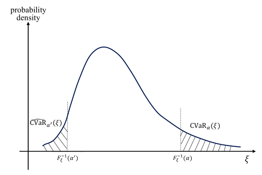
Figure 1: Illustration of right-tailed and left-tailed definitions of CVaR.

In this paper, the $\mathrm{CVaR}$ of $\xi$ at probability level $\alpha$ is defined as the expectation of the $(1-\alpha)$-tail distribution of $\xi$, i.e.,

$$\mathrm{CVaR}_{\alpha}(\xi):=\frac{1}{1-\alpha}\int_{\alpha}^{1}\mathrm{VaR}_{q}(\xi)d{q}.$$ (1)

As illustrated by Fig. 1, (1) is a right-tailed definition of CVaR, and there also exists another definition of CVaR focusing on the left-tailed distribution, i.e.,

$$\widehat{\mathrm{CVaR}}_{\alpha}(\xi):=\frac{1}{\alpha}\int_{0}^{\alpha}\mathrm{VaR}_{q}(\xi)d{q}.$$

Obviously, we can derive the following relations

$$\mathrm{CVaR}_{\alpha}(\xi)=-\widehat{\mathrm{CVaR}}_{1-\alpha}(-\xi),$$

$$(1-\alpha)\mathrm{CVaR}_{\alpha}(\xi)+\alpha\widehat{\mathrm{CVaR}}_{\alpha}(\xi)=\mathbbm{E}[\xi].$$

Therefore, maximizing (or minimizing) the right-tailed CVaR is equivalent to minimizing (or maximizing) the left-tailed CVaR. In the rest of this paper, we limit our discussion on the maximization of the right-tailed CVaR defined in (1).

Moreover, Rockafellar and Uryasev (2002) discovered that $\mathrm{CVaR}$ is equivalent to solving a convex optimization problem as follows.

$$\mathrm{CVaR}_{\alpha}(\xi)=\min_{y\in\mathbbm{R}}\left\{y+\frac{1}{1-\alpha}\mathbbm{E}[\xi-y]^{+}\right\},$$

where $[\xi-y]^{+}=\max\left\{\xi-y,0\right\}$, and $y^{*}=\mathrm{VaR}_{\alpha}(\xi)$ exactly attains the above minimum. Note that, if $\xi$ has lower bound $L$ and upper bound $U$, we can further specify the domain $y\in\mathbbm{R}$ to a bounded set $[L,U]$, i.e.,

$$\mathrm{CVaR}_{\alpha}(\xi)=\min_{y\in[L,U]}\left\{y+\frac{1}{1-\alpha}\mathbbm{E}[\xi-y]^{+}\right\}.$$ (2)

As aforementioned, we focus on the maximization of CVaR in this paper, which reflects the risk-seeking preference of decision makers. Risk-averse optimization has been widely studied in the literature. Meanwhile, risk seeking is also an important attitude of decision makers (Armstrong and Brigo, 2019), but much less research attention has been paid to on this topic. According to the prospect theory (Kahneman and Tversky, 1979), decision makers usually present risk-seeking attitude in the loss frame (negative prospect). As illustrated in Fig. 2, people tend to choose a risky gamble (Case A) rather than a sure loss (Case B). Obviously, Case A has a larger value of CVaR. Such kind of risk-seeking behaviors can also be found among casino-goers who pursue extreme rewards although the expectation is negative. Even in reinforcement learning, an optimization goal including risk-seeking metrics may enable the algorithm a stronger exploratory capability to find better solutions (Dilokthanakul and Shanahan, 2019; Mihatsch and Neuneier, 2002). However, to the best of our knowledge, there is no literature on the risk-seeking optimization of CVaR in dynamic scenarios. Thus, it is of significance to study the maximization of CVaR in MDPs.

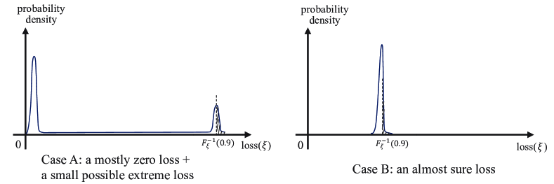
Figure 2: Risk-seeking attitude in losses according to the prospect theory, where Case A is preferred with a larger CVaR risk value.

2.2 Markov Decision Process

A discrete-time average MDP can be denoted by a tuple $\mathcal{M}:=\langle\mathcal{S},\mathcal{A},(\mathcal{A}(s),s\in\mathcal{S}),\bm{P},\bm{r}\rangle$, where $\mathcal{S}$ and $\mathcal{A}$ represent the finite state and action spaces, respectively; $\mathcal{A}(s)$ is the set of the admissible actions at state $s$ and we have $\bigcup\limits_{s\in\mathcal{S}}\mathcal{A}(s)=\mathcal{A}$; $\bm{P}$ denotes the Markov kernel, and its element $P(\cdot|s,a)$ is a probability measure on $\mathcal{S}$ for each given $(s,a)\in\mathcal{K}$ where $\mathcal{K}:=\left\{(s,a):s\in\mathcal{S},a\in\mathcal{A}(s)\right\}$; and $\bm{r}:\mathcal{K}\rightarrow\mathbbm{R}$ is the reward function with the minimum $L_{r}$ and the maximum $U_{r}$.

The discrete-time MDP evolves as follows. Suppose the system state is $s_{t}\in\mathcal{S}$ at the current time $t$, and an action $a_{t}\in\mathcal{A}(s_{t})$ is adopted based on a policy $u$. The system will receive an instantaneous reward $R_{t}:=r(s_{t},a_{t})$, and then move to a new state $s_{t+1}\in\mathcal{S}$ at the next time $t+1$ according to the transition probability $P(s_{t+1}|s_{t},a_{t})$. The policy $u$ prescribes the action-selection rule at each decision time epoch based on either history or just the current state, where the former refers to a history-dependent randomized policy while the latter refers to a Markov randomized policy. Specifically, a history-dependent randomized policy is a sequence of stochastic kernels, i.e., $u:=(u_{t},t\geq 0)$, where $u_{t}(\cdot|h_{t})$ is a probability measure on $\mathcal{A}$ for given history $h_{t}:=\left\{s_{0},a_{0},\ldots,s_{t-1},a_{t-1},s_{t}\right\}$. If $u_{t}(\cdot|h_{t})=u_{t}(\cdot|s_{t})$, $\forall h_{t}$, we call $u$ a Markov randomized policy which only depends on the current state $s_{t}$. Furthermore, if $u_{t}$ is independent of the decision time $t$, i.e., there exists a stochastic kernel $d$ on $\mathcal{A}$ given $\mathcal{S}$ such that $d(\cdot|s_{t})=u_{t}(\cdot|s_{t}),\forall t\geq 0$, we call $d^{\infty}:=(d,d,\cdots)$ or simply $d$ a stationary randomized policy. For notational simplicity, we denote the sets of all the history-dependent randomized policies, the Markov randomized policies, and the stationary randomized policies by $\mathbbm{U}$, $\mathbbm{U}^{\rm MR}$, and $\mathbbm{D}$, respectively.

For each initial state $s\in\mathcal{S}$ and policy $u\in\mathbbm{U}$, by the Theorem of C. Ionescu-Tulcea (Hernández-Lerma and Lasserre, 1996, P.178), there exists a unique probability measure $\mathbbm{P}_{s}^{u}$ on the space of trajectories of the states and actions such that $\mathbbm{P}_{s}^{u}(s_{0},a_{0},s_{1},a_{1},\ldots)=\delta_{s}(s_{0})u_{0}(a_{0}|s_{0})\\ P(s_{1}|s_{0},a_{0})u_{1}(a_{1}|s_{0},a_{0},s_{1})\cdots$, where $\delta$ denotes the Dirac measure.

2.3 Definition of Long-Run CVaR Criterion

In this paper, we focus on the long-run CVaR criterion in discrete-time MDPs. We give a rigorous definition as follows, where the probability level $\alpha\in(0,1)$ is assumed fixed.

Definition 1.

For each initial state $s\in\mathcal{S}$ and policy $u\in\mathbbm{U}$, let $R^{s,u}_{t}$ be the instantaneous reward at time $t$, the limsup long-run CVaR is defined as

$$\mathrm{CVaR}^{u}_{+}(s):=\limsup\limits_{T\rightarrow\infty}{\frac{1}{T}{\sum\limits_{t=0}^{T-1}}}\mathrm{CVaR}_{\alpha}\big{(}R^{s,u}_{t}\big{)},$$ (3)

and the liminf long-run CVaR is defined as

$$\mathrm{CVaR}^{u}_{-}(s):=\liminf\limits_{T\rightarrow\infty}{\frac{1}{T}{\sum\limits_{t=0}^{T-1}}}\mathrm{CVaR}_{\alpha}\big{(}R^{s,u}_{t}\big{)}.$$ (4)

If it holds that $\mathrm{CVaR}^{u}_{+}(s)=\mathrm{CVaR}^{u}_{-}(s)$ for some $u\in\mathbbm{U}$ and each $s\in\mathcal{S}$, the common function is called the long-run CVaR and denoted by $\mathrm{CVaR}^{u}(s)$, i.e.,

$$\mathrm{CVaR}^{u}(s):=\lim\limits_{T\rightarrow\infty}{\frac{1}{T}{\sum\limits_{t=0}^{T-1}}}\mathrm{CVaR}_{\alpha}\big{(}R^{s,u}_{t}\big{)}.$$ (5)

For notational simplicity, we denote by $\hat{\mathbbm{U}}$ the set of all policies that make (5) well defined, i.e., $\mathrm{CVaR}^{u}_{+}(s)=\mathrm{CVaR}^{u}_{-}(s),\forall u\in\hat{\mathbbm{U}}$.

Remark 1.

To make the dependence on the initial state $s$ explicit, we write $R^{s,u}_{t}$ as the per-step reward, which is a bounded-mean random variable with support on $\left\{{r}(i,a):(i,a)\in\mathcal{K}\right\}$ and the corresponding probability distribution is $\mathbbm{P}^{u,t}_{s}(i,a)=\mathbbm{P}^{u}_{s}(s_{t}=i,a_{t}=a)$. Considering that the limit of (5) may not exist (see Example 1 in Section 6 for instance), we derive two related quantities as (3) and (4), which is similar to average MDPs (Puterman, 1994). Furthermore, (5) is well defined for stationary randomized policies $u\in\mathbbm{D}$, as later Theorem 1 illustrates.

With the definitions of (3)-(5), we define the corresponding MDP optimization problems for these CVaR metrics, respectively.

Definition 2.

We define the following CVaR maximization problems in MDPs

$$\mathrm{CVaR}^{u^{*}_{+}}_{+}(s) = \sup\limits_{u\in\mathbbm{U}}\mathrm{CVaR}^{u}_{+}(s),\qquad\forall s\in\mathcal{S},$$ (6)

$$\mathrm{CVaR}^{u^{*}_{-}}_{-}(s) = \sup\limits_{u\in\mathbbm{U}}\mathrm{CVaR}^{u}_{-}(s),\qquad\forall s\in\mathcal{S},$$ (7)

$$\mathrm{CVaR}^{u^{*}}(s) = \sup\limits_{u\in\hat{\mathbbm{U}}}\mathrm{CVaR}^{u}(s),\qquad\forall s\in\mathcal{S},$$ (8)

where $u^{*}_{+}$, $u^{*}_{-}$, and $u^{*}$ are called the limsup-optimal, liminf-optimal, and optimal policies for the long-run CVaR maximization problem of MDPs, respectively.

For notational simplicity, we denote $\mathrm{CVaR}^{*}_{+}(\cdot):=\mathrm{CVaR}^{u^{*}_{+}}_{+}(\cdot)$, $\mathrm{CVaR}^{*}_{-}(\cdot):=\mathrm{CVaR}^{u^{*}_{-}}_{-}(\cdot)$, and $\mathrm{CVaR}^{*}(\cdot):=\mathrm{CVaR}^{u^{*}}(\cdot)$. Note that, the policy set $\hat{\mathbbm{U}}$ is difficult to determine since it requires $\mathrm{CVaR}^{u}_{+}(s)=\mathrm{CVaR}^{u}_{-}(s)$ for any $u\in\hat{\mathbbm{U}}$. Fortunately, we further discover that the optima of these three problems (6)-(8) are the same and can be attained by a common stationary randomized policy $d^{*}\in\mathbbm{D}$.

3 Existence of Optimal Stationary Randomized Policy

First, we derive the following lemma to show that the optimality of Markov randomized policies for these long-run CVaR MDP problems.

Lemma 1.

For any given $s\in\mathcal{S}$, the optima $\mathrm{CVaR}^{*}_{+}(s)$, $\mathrm{CVaR}^{*}_{-}(s)$, and $\mathrm{CVaR}^{*}(s)$ in (6)-(8) can be attained by Markov randomized policies in $\mathbbm{U}^{\rm MR}$, respectively.

Proof.

We first prove the statement for $\mathrm{CVaR}^{*}(s)$, other statements for limsup and liminf optimum can be proved with the same argument.

We fix $s\in\mathcal{S}$. For each given $u\in\mathbbm{U}$, using the property (2), we have

$$\mathrm{CVaR}_{\alpha}\big{(}R^{s,u}_{t}\big{)} =\min_{y\in\mathbbm{Y}}\left\{y+\frac{1}{1-\alpha}\mathbbm{E}[R^{s,u}_{t}-y]^{+}\right\}$$

$$=\min_{y\in\mathbbm{Y}}\left\{y+\frac{1}{1-\alpha}\sum\limits_{(i,a)\in\mathcal{K}}\mathbbm{P}^{u,t}_{s}(i,a)[r(i,a)-y]^{+}\right\},$$ (9)

where $\mathbbm{Y}:=[L_{r},U_{r}]$. With Theorem 5.5.1 of Puterman (1994), there exists a policy $u^{\prime}\in\mathbbm{U}^{\rm MR}$ such that the associated Markov chains have the same $t$-step distribution, i.e.,

$$\mathbbm{P}^{u^{\prime},t}_{s}(i,a)=\mathbbm{P}^{u,t}_{s}(i,a),\quad\forall t\geq 0,~{}(i,a)\in\mathcal{K}.$$ (10)

Substituting (3) and (10) into (5), we derive

$$\mathrm{CVaR}^{u^{\prime}}(s)=\mathrm{CVaR}^{u}(s),$$ (11)

whenever the RHS (right-hand-side) of (11) is well defined. Thus, Lemma 1 holds. ∎

With Lemma 1, we can restrict the policy searching space of (6)-(8) from $\mathbbm{U}$ to $\mathbbm{U}^{\rm MR}$. By imposing the following assumption of unichain and aperiodicity, we can further restrict our attention to stationary randomized policy space $\mathbbm{D}$.

Assumption 1.

For each $d\in\mathbbm{D}$, the Markov chain under policy $d$ is unichain and aperiodic.

Assumption 1 indicates that the Markov chain $\left\{s_{t},~{}t\geq 0\right\}$ tends to be steady as $t\rightarrow\infty$ (Puterman, 1994). That is, the limiting distribution of the discrete-time MDP under policy $d\in\mathbbm{D}$ is well defined

$$\pi^{d}(i,a):=\lim\limits_{t\rightarrow\infty}\mathbbm{P}^{d,t}_{s}(i,a),\quad\forall s\in\mathcal{S},~{}(i,a)\in\mathcal{K},$$ (12)

which also satisfies the following stationary distribution equation

$$\begin{cases}\sum\limits_{a\in\mathcal{A}(j)}\pi^{d}(j,a)=\sum\limits_{(i,a)\in\mathcal{K}}P(j\mid i,a)\pi^{d}(i,a),\quad\forall j\in\mathcal{S};\\ \sum\limits_{(i,a)\in\mathcal{K}}\pi^{d}(i,a)=1;~{}~{}~{}~{}~{}~{}~{}\pi^{d}(i,a)\geq 0,\quad\forall(i,a)\in\mathcal{K}.\end{cases}$$ (13)

For notational simplicity, we denote $\mathbbm{X}$ as the set of vectors $\bm{x}\in\mathbbm{R}^{\lvert\mathcal{K}\rvert}$ satisfying (13), where we replace $\pi^{d}$ with $x$. We call $\mathbbm{X}$ the set of feasible solutions of steady-state distribution of the MDP, and each $\bm{x}\in\mathbbm{X}$ indicates the steady-state distribution of the MDP under a particular randomized policy $d\in\mathbbm{D}$.

Since $R^{s,d}_{t}$ follows the distribution $\mathbbm{P}^{d,t}_{s}$, (12) indicates $R^{s,d}_{t}\stackrel{{\scriptstyle L}}{{\longrightarrow}}R^{d}$ (convergence in distribution), where $R^{d}$ is a random variable defined with support on $\left\{{r}(i,a):(i,a)\in\mathcal{K}\right\}$ and corresponding probability distribution $\bm{\pi}^{d}$. Next, we derive Lemma 2 to establish the equivalence between $\mathrm{CVaR}_{\alpha}(R^{s,d}_{t})$ and $\mathrm{CVaR}_{\alpha}(R^{d})$.

Lemma 2.

For each initial state $s\in\mathcal{S}$ and stationary randomized policy $d\in\mathbbm{D}$, it holds that

$$\lim\limits_{t\rightarrow\infty}\mathrm{CVaR}_{\alpha}\big{(}R^{s,d}_{t}\big{)}=\mathrm{CVaR}_{\alpha}\big{(}R^{d}\big{)}.$$ (14)

Proof.

We use the alternative representation (2) of $\mathrm{CVaR}$ to estimate the gap between $\mathrm{CVaR}_{\alpha}(R^{s,d}_{t})$ and $\mathrm{CVaR}_{\alpha}(R^{d})$.

$$\bigg{\lvert}\mathrm{CVaR}_{\alpha}\big{(}R^{s,d}_{t}\big{)}-\mathrm{CVaR}_{\alpha}\big{(}R^{d}\big{)}\bigg{\rvert} =\bigg{\lvert}\min_{y\in\mathbbm{Y}}\left\{y+\frac{1}{1-\alpha}\mathbbm{E}[R^{s,d}_{t}-y]^{+}\right\}-\min_{y\in\mathbbm{Y}}\left\{y+\frac{1}{1-\alpha}\mathbbm{E}[R^{d}-y]^{+}\right\}\bigg{\rvert}$$

$$\leq\frac{1}{1-\alpha}\max\limits_{y\in\mathbbm{Y}}\bigg{\lvert}\mathbbm{E}[R^{s,d}_{t}-y]^{+}-\mathbbm{E}[R^{d}-y]^{+}\bigg{\rvert}$$

$$=\frac{1}{1-\alpha}\max\limits_{y\in\mathbbm{Y}}\bigg{\lvert}\sum\limits_{(i,a)\in\mathcal{K}}[\mathbbm{P}^{d,t}_{s}(i,a)-\pi^{d}(i,a)][r(i,a)-y]^{+}\bigg{\rvert}$$

$$\leq\frac{1}{1-\alpha}\max\limits_{y\in\mathbbm{Y}}\sum\limits_{(i,a)\in\mathcal{K}}\big{\lvert}\mathbbm{P}^{d,t}_{s}(i,a)-\pi^{d}(i,a)\big{\rvert}[r(i,a)-y]^{+}$$

$$\leq\frac{U_{r}-L_{r}}{1-\alpha}\sum\limits_{(i,a)\in\mathcal{K}}\big{\lvert}\mathbbm{P}^{d,t}_{s}(i,a)-\pi^{d}(i,a)\big{\rvert},$$

where the first and second inequalities follow from $\lvert\min\limits_{y}f_{1}(y)-\min\limits_{y}f_{2}(y)\rvert\leq\max\limits_{y}\lvert{f_{1}(y)-f_{2}(y)}\rvert$ and the absolute value inequality, respectively, and the last inequality is ensured by the fact $[r(i,a)-y]^{+}\leq U_{r}-L_{r}$ for any $y\in\mathbbm{Y},(i,a)\in\mathcal{K}$. Thus, by using (12) and the finiteness of $\mathcal{K}$, we see that the gap in the above inequality goes to 0 as $t\rightarrow\infty$, and Lemma 2 holds. ∎

Remark 2.

Lemma 2 implies an important property of CVaR: The order of CVaR measure and the limit of $t$ is interchangeable, i.e.,

$$\lim\limits_{t\rightarrow\infty}\mathrm{CVaR}_{\alpha}\big{(}\xi_{t}\big{)}=\mathrm{CVaR}_{\alpha}\big{(}\xi\big{)},$$ (15)

if $\left\{\xi_{t}\right\}$ is a series of bounded discrete-valued random variables with $\xi_{t}\stackrel{{\scriptstyle L}}{{\longrightarrow}}\xi$. Furthermore, $(\ref{equ:conver})$ also holds if $\xi_{t}\stackrel{{\scriptstyle P}}{{\longrightarrow}}\xi$ (convergence in probability) or $\xi_{t}\stackrel{{\scriptstyle a.s.}}{{\longrightarrow}}\xi$ (almost sure convergence) since both of them imply $\xi_{t}\stackrel{{\scriptstyle L}}{{\longrightarrow}}\xi$.

Below, we give an important consequence of Lemma 2.

Lemma 3.

For any initial state $s\in\mathcal{S}$ and stationary randomized policy $d\in\mathbbm{D}$, the limsup, liminf, and long-run CVaR defined in (3)-(5) all equal the CVaR of $R^{d}$, i.e.,

$$\mathrm{CVaR}^{d}_{+}(s)=\mathrm{CVaR}^{d}_{-}(s)=\mathrm{CVaR}^{d}(s)=\mathrm{CVaR}_{\alpha}\big{(}R^{d}\big{)},\qquad\forall s\in\mathcal{S},~{}d\in\mathbbm{D}.$$ (16)

Proof.

Since $\lim\limits_{t\rightarrow\infty}\mathrm{CVaR}_{\alpha}\big{(}R^{s,d}_{t}\big{)}=\mathrm{CVaR}_{\alpha}\big{(}R^{d}\big{)}$, the limit of (5) exists and further

$$\mathrm{CVaR}^{d}(s)=\lim\limits_{T\rightarrow\infty}{\frac{1}{T}{\sum\limits_{t=0}^{T-1}}}\mathrm{CVaR}_{\alpha}\big{(}R^{s,d}_{t}\big{)}=\mathrm{CVaR}_{\alpha}\big{(}R^{d}\big{)}.$$

Since $\mathrm{CVaR}^{d}(s)$ in (5) is well defined as above, it implies that $\mathrm{CVaR}^{d}_{+}(s)=\mathrm{CVaR}^{d}_{-}(s)=\mathrm{CVaR}^{d}(s)$. Thus, the lemma is proved. ∎

Next, we focus on the optimization analysis of the long-run CVaR maximization in MDPs, as defined in (6)-(8). We find that the optimality of stationary randomized policies is guaranteed, as stated by Theorem 1.

Theorem 1.

The optima $\mathrm{CVaR}^{*}_{+}(s)$, $\mathrm{CVaR}^{*}_{-}(s)$, and $\mathrm{CVaR}^{*}(s)$ in (6)-(8) over the set of history-dependent randomized policies can be attained by a stationary randomized policy $d^{*}\in\mathbbm{D}$, i.e.,

$$\mathrm{CVaR}^{*}_{+}(s)=\mathrm{CVaR}^{*}_{-}(s)=\mathrm{CVaR}^{*}(s)=\mathrm{CVaR}^{d^{*}}(s),\quad\forall s\in\mathcal{S},$$ (17)

where $d^{*}$ is attained by

$$d^{*}\in\operatorname*{argmax}\limits_{d\in\mathbbm{D}}\mathrm{CVaR}_{\alpha}\big{(}R^{d}\big{)}.$$ (18)

Proof.

By using Lemma 3, we just need to prove

$$\mathrm{CVaR}^{*}(s)=\max\limits_{d\in\mathbbm{D}}\mathrm{CVaR}_{\alpha}\big{(}R^{d}\big{)},\quad\forall s\in\mathcal{S},$$

which is equivalent to prove

$$\mathrm{CVaR}^{*}_{+}(s)\leq\max\limits_{d\in\mathbbm{D}}\mathrm{CVaR}_{\alpha}\big{(}R^{d}\big{)},\quad\forall s\in\mathcal{S},$$ (19)

and

$$\mathrm{CVaR}^{*}_{-}(s)\geq\max\limits_{d\in\mathbbm{D}}\mathrm{CVaR}_{\alpha}\big{(}R^{d}\big{)},\quad\forall s\in\mathcal{S}.$$ (20)

First, we prove (20). Since $\mathbbm{D}\subset\mathbbm{U}^{\rm MR}$, we have

$$\mathrm{CVaR}^{*}_{-}(s)=\sup\limits_{u\in\mathbbm{U}^{\rm MR}}\mathrm{CVaR}^{u}_{-}(s)\geq\max\limits_{d\in\mathbbm{D}}\mathrm{CVaR}^{d}_{-}(s)=\max\limits_{d\in\mathbbm{D}}\mathrm{CVaR}_{\alpha}\big{(}R^{d}\big{)},$$

where the first equality follows from Lemma 1 and the last one follows from (16).

Next, we prove (19). For any $u\in\mathbbm{U}^{\rm MR}$ and $s\in\mathcal{S}$, using the property (2), we have

$$\mathrm{CVaR}^{u}_{+}(s) =\limsup\limits_{T\rightarrow\infty}{\frac{1}{T}{\sum\limits_{t=0}^{T-1}}}\mathrm{CVaR}_{\alpha}\big{(}R^{s,u}_{t}\big{)}$$

$$=\limsup\limits_{T\rightarrow\infty}{\frac{1}{T}{\sum\limits_{t=0}^{T-1}}}\min_{y\in\mathbbm{Y}}\left\{y+\frac{1}{1-\alpha}\mathbbm{E}[R^{s,u}_{t}-y]^{+}\right\}$$

$$\leq\min_{y\in\mathbbm{Y}}\limsup\limits_{T\rightarrow\infty}{\frac{1}{T}{\sum\limits_{t=0}^{T-1}}}\left\{y+\frac{1}{1-\alpha}\mathbbm{E}[R^{s,u}_{t}-y]^{+}\right\}$$

$$=\min_{y\in\mathbbm{Y}}\left\{y+\frac{1}{1-\alpha}\limsup\limits_{T\rightarrow\infty}{\frac{1}{T}{\sum\limits_{t=0}^{T-1}}}\mathbbm{E}[R^{s,u}_{t}-y]^{+}\right\},$$

which yields

$$\mathrm{CVaR}^{*}_{+}(s)=\sup\limits_{u\in\mathbbm{U}^{\rm MR}}\mathrm{CVaR}^{u}_{+}(s)\leq\min\limits_{y\in\mathbbm{Y}}\left\{y+\frac{1}{1-\alpha}\sup\limits_{u\in\mathbbm{U}^{\rm MR}}\limsup\limits_{T\rightarrow\infty}{\frac{1}{T}{\sum\limits_{t=0}^{T-1}}}\mathbbm{E}[R^{s,u}_{t}-y]^{+}\right\},$$ (21)

where the equality follows from Lemma 1 and the inequality follows from $\sup\min\{\cdot\}\leq\min\sup\{\cdot\}$. Note that, the term $\limsup\limits_{T\rightarrow\infty}{\frac{1}{T}{\sum\limits_{t=0}^{T-1}}}\mathbbm{E}[R^{s,u}_{t}-y]^{+}$ in (21) is a standard MDP with average criterion for given $y\in\mathbbm{Y}$. By using the fact that $\mathbbm{D}$ remains optimal over $\mathbbm{U}^{\rm M}$ in average reward MDPs (refer to Theorem $8.4.5$ of Puterman (1994)), we directly have

$$\sup\limits_{u\in\mathbbm{U}^{\rm MR}}\limsup\limits_{T\rightarrow\infty}{\frac{1}{T}{\sum\limits_{t=0}^{T-1}}}\mathbbm{E}[R^{s,u}_{t}-y]^{+}=\max\limits_{d\in\mathbbm{D}}\lim\limits_{T\rightarrow\infty}{\frac{1}{T}{\sum\limits_{t=0}^{T-1}}}\mathbbm{E}[R^{s,d}_{t}-y]^{+}=\max\limits_{d\in\mathbbm{D}}\sum\limits_{(i,a)\in\mathcal{K}}\pi^{d}(i,a)[r(i,a)-y]^{+}.$$

Substituting the above equation into (21), we have

$$\mathrm{CVaR}^{*}_{+}(s) \leq\min\limits_{y\in\mathbbm{Y}}\left\{y+\frac{1}{1-\alpha}\max\limits_{d\in\mathbbm{D}}\sum\limits_{(i,a)\in\mathcal{K}}\pi^{d}(i,a)[r(i,a)-y]^{+}\right\}$$

$$=\min\limits_{y\in\mathbbm{Y}}\max\limits_{d\in\mathbbm{D}}\left\{y+\frac{1}{1-\alpha}\sum_{(i,a)\in\mathcal{K}}\pi^{d}(i,a)[r(i,a)-y]^{+}\right\}.$$

Note that the above $\min\max\{\cdot\}$ is interchangeable by using Lemma 4 shown later, thus

$$\mathrm{CVaR}^{*}_{+}(s)\leq\max\limits_{d\in\mathbbm{D}}\min\limits_{y\in\mathbbm{Y}}\left\{y+\frac{1}{1-\alpha}\sum\limits_{(i,a)\in\mathcal{K}}\pi^{d}(i,a)[r(i,a)-y]^{+}\right\}=\max\limits_{d\in\mathbbm{D}}\mathrm{CVaR}_{\alpha}\big{(}R^{d}\big{)}.$$

The above analysis completes the proof of Theorem 1. ∎

Remark 3.

With Lemma 1 and Theorem 1, the optimality of Markov randomized policy and stationary randomized policy is guaranteed, respectively. We can limit our policy searching space to $\mathbbm{U}^{\rm MR}$, and eventually to $\mathbbm{D}$, which significantly reduces the optimization complexity. Thus, the original long-run CVaR maximization problems (6)-(8) are equivalent to solving (18) over the stationary randomized policy space $\mathbbm{D}$.

By using (2), we find that solving (18) over $\mathbbm{D}$ can be transformed to the following mathematical program

$$\max\limits_{d\in\mathbbm{D}}\mathrm{CVaR}_{\alpha}\big{(}R^{d}\big{)} =\max\limits_{d\in\mathbbm{D}}\min_{y\in\mathbbm{Y}}\left\{y+\frac{1}{1-\alpha}\mathbbm{E}\big{[}R^{d}-y\big{]}^{+}\right\}$$

$$=\max_{d\in\mathbbm{D}}\min_{y\in\mathbbm{Y}}\sum_{(i,a)\in\mathcal{K}}\pi^{d}(i,a)\left\{y+\frac{1}{1-\alpha}[r(i,a)-y]^{+}\right\}$$

$$=\max_{\bm{x}\in\mathbbm{X}}\min_{y\in\mathbbm{Y}}\sum_{(i,a)\in\mathcal{K}}x(i,a)\left\{y+\frac{1}{1-\alpha}[r(i,a)-y]^{+}\right\},$$ (22)

where $\mathbbm{X}$ is determined by (13). For notational simplicity, we define

$$v(\bm{x},y):=\sum_{(i,a)\in\mathcal{K}}x(i,a)\left\{y+\frac{1}{1-\alpha}[r(i,a)-y]^{+}\right\}.$$ (23)

Thus, the CVaR maximization problem $(\ref{equ:max_CVaR})$ can be simply rewritten as

$$\max_{\bm{x}\in\mathbbm{X}}\min_{y\in\mathbbm{Y}}v(\bm{x},y).$$ (24)

Interestingly, we discover that (24) is a saddle point problem by using the von Neumann minimax theorem (Barron, 2013, Theorem 1.2.3), and derive the following lemma

Lemma 4.

There exists at least one saddle point solution of (24), and it holds that

$$\max_{\bm{x}\in\mathbbm{X}}\min_{y\in\mathbbm{Y}}v(\bm{x},y)=\min_{y\in\mathbbm{Y}}\max_{\bm{x}\in\mathbbm{X}}v(\bm{x},y).$$ (25)

The common value is denoted as $v^{*}$. Furthermore, a pair $(\bm{x}^{*},y^{*})\in\mathbbm{X}\times\mathbbm{Y}$ is said to be a saddle point solution if and only if

$$v(\bm{x},y^{*})\leq v(\bm{x}^{*},y^{*})=v^{*}\leq v(\bm{x}^{*},y),\quad\forall(\bm{x},y)\in\mathbbm{X}\times\mathbbm{Y}.$$

Proof.

Note that both $\mathbbm{X}$ and $\mathbbm{Y}$ are convex, closed and bounded. In order to apply the von Neumann minimax theorem, we just need to verify that $v(\bm{x},y)$ is concave in $\bm{x}$ and convex in $y$. The concavity in $\bm{x}$ follows directly from the linearity of $\bm{x}$ in (23). The convexity in $y$ is easily verified in (23) (Rockafellar and Uryasev, 2002). Thus, the lemma holds. ∎

Lemma 4 indicates that the long-run CVaR maximization of MDPs under stationary randomized policies can be reduced to a solvable saddle point problem (25), which exactly motivates the development of optimization algorithms in Section 4. From the right-hand-side of (25), we can see that for any given $y$, the inner problem $\max\limits_{\bm{x}\in\mathbbm{X}}v(\bm{x},y)$ is actually a standard MDP. Thus, solving (25) can be viewed as a bilevel MDP problem solving a series of MDPs, which is computationally intensive. Below, we further discuss the structural property of optimal policies, which is useful for us to develop computationally efficient algorithms.

It is well known that the optimality of stationary deterministic policies is guaranteed for classical MDPs with expected discounted or average criteria (Puterman, 1994). Such optimality also holds for some risk-averse criteria including variance-related criterion (Sobel, 1994; Xia, 2020) and discounted CVaR criterion (Haskell and Jain, 2015; Huang and Guo, 2016). For long-run CVaR minimization criterion in MDPs, the optimality of deterministic policies is also proved by Xia and Glynn (2022). However, this seemingly universal result cannot be extended to our long-run CVaR maximization MDP, which is demonstrated by a counterexample, refer to Example 2 in Section 6. Thus, we make the following statement

Proposition 1.

The optimum of the long-run CVaR maximization MDP may not be attainable by a stationary deterministic policy.

In order to further explore the structural property of optimal policies, we introduce the concept of the “number of randomizations” to measure the randomness of policies.

Definition 3.

The number of randomizations of state $i\in\mathcal{S}$ under policy $d\in\mathbbm{D}$ is $m(i,d)$, if there are exactly $m(i,d)+1$ actions $a$ in $\mathcal{A}(i)$ such that $d(a|i)>0$. Further, the number of randomizations under policy $d$ is defined as

$$n(d):=\sum_{i\in\mathcal{S}}m(i,d).$$

Definition 3 was originally proposed by Altman (1999) to study the structural property of optimal policies in constrained MDPs. We show the existence of an optimal stationary randomized policy that requires at most one randomization, as Theorem 2 states.

Theorem 2.

There exists an optimal stationary randomized policy $d^{*}\in\mathbbm{D}$ of the long-run CVaR maximization MDP such that the number of randomizations under $d^{*}$ is at most one, i.e., $n(d^{*})\leq 1$.

Proof.

Suppose $(\bm{x}^{*},y^{*})$ is a saddle point of (25) and let $d^{*}\in\mathbbm{D}$ be the corresponding optimal policy. Noting that $y=\mathrm{VaR}_{\alpha}(\xi)$ attains the minimum of (2), we can see that $y^{*}=\mathrm{VaR}_{\alpha}(R^{d^{*}})$. By the definition of $\mathrm{VaR}$, we have

$$y^{*}=\inf\left\{z\in\mathbbm{R}:\mathbbm{P}(R^{d^{*}}\leq z)\geq\alpha\right\}.$$ (26)

(26) implies two facts:

$$\mathbbm{P}(R^{d^{*}}\leq y^{*})\geq\alpha,$$ (27)

$$\mathbbm{P}(R^{d^{*}}\leq y^{*-})<\alpha.$$ (28)

Obviously, $\mathrm{VaR}_{\alpha}(R^{d^{*}})$ must belong to the set $\left\{r(i,a):(i,a)\in\mathcal{K}\right\}$. Thus, $y^{*}\in\left\{r(i,a):(i,a)\in\mathcal{K}\right\}$. We sort $\left\{r(i,a):(i,a)\in\mathcal{K}\right\}$ in ascending order and denote the minimum distance between any two adjacent rewards $r(i,a)$’s as $\delta$. Since $R^{d^{*}}$ is a discrete random variable, (28) is equivalent to

$$\mathbbm{P}(R^{d^{*}}\leq y^{*}-\delta)<\alpha.$$ (29)

Now, we represent (27) and (29) in expectation forms by using indicator function as below

$$\sum\limits_{(i,a)\in\mathcal{K}}x^{*}(i,a)\mathbbm{1}\left\{r(i,a)\leq y^{*}\right\}\geq\alpha,$$

$$\sum\limits_{(i,a)\in\mathcal{K}}x^{*}(i,a)\mathbbm{1}\left\{r(i,a)\leq y^{*}-\delta\right\}<\alpha.$$

Given $y^{*}$, the optimal policy $d^{*}$ (corresponding to $\bm{x}^{*}$) can be regarded as an optimal solution of the following linear program

$$\max_{\bm{x}}\quad\sum_{(i,a)\in\mathcal{K}}x(i,a)\left\{y^{*}+\frac{1}{1-\alpha}[r(i,a)-y^{*}]^{+}\right\}$$

$$\begin{array}[]{r@{\quad}l@{}l@{\quad}l}s.t.&-\sum\limits_{(i,a)\in\mathcal{K}}x(i,a)\mathbbm{1}\left\{r(i,a)\leq y^{*}\right\}\leq-\alpha\\ &\sum\limits_{(i,a)\in\mathcal{K}}x(i,a)\mathbbm{1}\left\{r(i,a)\leq y^{*}-\delta\right\}+x_{0}=\alpha\\ &\bm{x}\in\mathbbm{X},~{}x_{0}>0,\end{array}$$ (33)

where $x_{0}$ is a slack variable. The structure of the optimal solution can be analyzed from the perspective of linear programming as follows.

First, Theorem 1 implies that linear program (3) is feasible. It is worth noting that linear program (3) contains at most $\lvert\mathcal{S}\rvert+2$ independent constraints. This implies that there exists an optimal solution $\tilde{\bm{x}}^{*}:=\left\{\bm{x}^{*},x^{*}_{0}\right\}$ for this linear program that has at most $\lvert\mathcal{S}\rvert+2$ non-zero elements. Recall that $x^{*}_{0}$ must be positive when it attains optimum, it follows that $\bm{x}^{*}$ has at most $\lvert\mathcal{S}\rvert+1$ non-zero elements. Based on the assumption of ergodic property, we also have $\sum\limits_{a\in\mathcal{A}(i)}{x}^{*}(i,a)>0$ for each $i\in\mathcal{S}$. Thus, there exists at most one state $i_{0}\in\mathcal{S}$ such that ${x}^{*}(i_{0},a_{1})>0$ and ${x}^{*}(i_{0},a_{2})>0$ for two different actions $a_{1},a_{2}\in\mathcal{A}(i_{0})$. Suppose $d^{*}$ is the optimal policy corresponding to this $\bm{x}^{*}$. According to Definition 3, the number of randomizations under $d^{*}$ is at most one. ∎

Note that the necessity of the randomization of optimal policies can be understood to increase the diversity of system behaviors, which is better for risk seeking. This randomization will vanish if we consider CVaR minimization instead of maximization, since deterministics is better for reducing risk. As a consequence of Theorem 2, the number of randomizations under $d^{*}$ must be $0$ or $1$. When $n(d^{*})=0$, it indicates stationary deterministic policies can preserve the optimality, which brings advantages for algorithmic study since the searching space is finite. When $n(d^{*})=1$, we have to consider stationary randomized policies, which brings challenges to algorithms since the searching space is infinite. In the next section, we discuss how to find the optimal policy for this long-run CVaR maximization MDP, based on the special form of the saddle point problem (25) and the structural properties of optimal policies stated by Theorems 1 and 2.

4 Algorithm

With the results in the previous section, we see that the long-run CVaR maximization MDPs (6)-(8) are equivalent to (18), further equivalent to the saddle point problem (25). For solving a general saddle point problem, we may use subgradient method to do iterative approximation (see, for instance, Nedić and Ozdaglar (2009) and the references therein), but it suffers from local convergence. In this section, considering the special form of the convex-concave function $v(\bm{x},y)$ in (23), we develop a global algorithm by formulating (25) as two linear programs.

With Lemma 4, the saddle point problem (25) is equivalent to a general dual pair of mathematical programs as below (Stoer, 1963).

$$\mbox{(mathematical program): \hskip 28.45274pt }\begin{array}[]{ll}&\min\limits_{y,z_{1}}\quad z_{1}\\ &\mbox{s.t.}\left\{\begin{array}[]{lr}v(\bm{x},y)\leq z_{1},\quad\forall\bm{x}\in\mathbbm{X},\\ y\in\mathbbm{Y}.\end{array}\right.\end{array}$$ (34)

$$\mbox{(dual program): \hskip 79.6678pt }\begin{array}[]{ll}&\max\limits_{\bm{x},z_{2}}\quad z_{2}\\ &\mbox{s.t.}\left\{\begin{array}[]{lr}v(\bm{x},y)\geq z_{2},\quad\forall y\in\mathbbm{Y},\\ \bm{x}\in\mathbbm{X}.\end{array}\right.\end{array}$$ (35)

Note that, the two mathematical programs are unsolvable due to nonlinearity of $v(\bm{x},y)$ and infinite constraints. However, the mathematical program (34) and dual program (35) can be reduced to two linear programs with finite constraints based on the property of convex-concave function $v(\bm{x},y)$ in (23).

Lemma 5.

The function $y\rightarrow v(\bm{x},y)$ is piecewise linear with endpoints $\left\{r(i,a):(i,a)\in\mathcal{K}\right\}$.

Lemma 5 indicates that $v(\bm{x},y)$ takes minimum at the endpoint set $\left\{r(i,a):(i,a)\in\mathcal{K}\right\}$ for any given $\bm{x}\in\mathbbm{X}$. Thus, the dual program (35) can be reduced to

$$\begin{array}[]{ll}&\max\limits_{\bm{x},z_{2}}\quad z_{2}\\ &\mbox{s.t.}\left\{\begin{array}[]{lr}v(\bm{x},r(i,a))\geq z_{2},\quad\forall(i,a)\in\mathcal{K},\\ x\in\mathbbm{X}.\end{array}\right.\end{array}$$ (36)

On the other hand, it is obvious that the function $\bm{x}\rightarrow v(\bm{x},y)$ is linear on $\mathbbm{X}$. Recall that $\mathbbm{X}$ is a bounded convex polyhedron. By the fundamental theorem of linear programming, each point of $\mathbbm{X}$ can be represented by the convex-combination of its vertices. Suppose $\left\{\bm{x}^{l}:l=1,2,\dots,L\right\}$ is the vertex set, which also refers to the basic feasible solution (BFS) set of feasible region $\mathbbm{X}$. Then for each $\bm{x}\in\mathbbm{X}$, there exist constants $\left\{\lambda_{l}:l=1,2,\dots,L\right\}$ with $0\leq\lambda_{l}\leq 1$ and $\sum\limits_{l=1}^{L}\lambda_{l}=1$ such that $\bm{x}=\sum\limits_{l=1}^{L}\lambda_{l}\bm{x}^{l}$. Thus, the mathematical program (34) can be reduced to

$$\begin{array}[]{ll}&\min\limits_{y,z_{1}}\quad z_{1}\\ &\mbox{s.t.}\left\{\begin{array}[]{lr}v(\bm{x}^{l},y)\leq z_{1},\quad\forall l=1,2,\ldots,L,\\ y\in\mathbbm{Y}.\end{array}\right.\end{array}$$ (37)

Taking the specific form of $v(\bm{x},y)$ in (23), (36) is obviously a standard linear program with variables $\bm{x}$ and $z_{2}$, while (37) contains a nonlinear term $[r(i,a)-y]^{+}$. It is worth noting that the nonlinear term can be removed by variable substitution. That is, we introduce new variables $w(i,a):=[r(i,a)-y]^{+}$ with added constraints $w(i,a)\geq 0$, $w(i,a)\geq r(i,a)-y$, $w(i,a)\leq r(i,a)-y+[1-b(i,a)](U_{r}-L_{r})$, $w(i,a)\leq b(i,a)(U_{r}-L_{r})$ and $b(i,a)\in\left\{0,1\right\}$. Through this transformation, (37) is expressed as a mixed-integer linear program (MILP):

$$\mbox{(MILP): \hskip 28.45274pt }\begin{array}[]{ll}&\min\limits_{y,z_{1},\bm{w},\bm{b}}\quad z_{1}\\ &\mbox{s.t.}\quad\left\{\begin{array}[]{lr}\sum\limits_{(i,a)\in\mathcal{K}}x^{l}(i,a)\big{[}y+\frac{1}{1-\alpha}w(i,a)\big{]}\leq z_{1},\quad l=1,2,\ldots,L\\ w(i,a)\geq r(i,a)-y,\quad\forall(i,a)\in\mathcal{K}\\ w(i,a)\geq 0,\quad\forall(i,a)\in\mathcal{K}\\ w(i,a)\leq r(i,a)-y+[1-b(i,a)](U_{r}-L_{r}),\quad\forall(i,a)\in\mathcal{K}\\ w(i,a)\leq b(i,a)(U_{r}-L_{r}),\quad\forall(i,a)\in\mathcal{K}\\ b(i,a)\in\left\{0,1\right\},\quad\forall(i,a)\in\mathcal{K}\\ L_{r}\leq y\leq U_{r}\end{array}\right.\end{array}$$ (38)

By noting that the coefficient $\frac{1}{1-\alpha}$ of the nonlinear term $[r(i,a)-y]^{+}$ is positive, we can further remove the $0-1$ variables $\left\{b(i,a)\right\}$ as well as the corresponding constraints in (38), since $w(i,a)$ must take endpoints $0$ or $r(i,a)-y$ when $z_{1}$ attains the minimum. Such a simplification cannot hold when the coefficient is negative. With this simplification, the original problems (34) and (35) are equivalent to the following two linear programs:

$$\mbox{(primal program): \hskip 28.45274pt }\begin{array}[]{ll}&\min\limits_{y,z_{1},\bm{w}}\quad z_{1}\\ &\mbox{s.t.}\quad\left\{\begin{array}[]{lr}\sum\limits_{(i,a)\in\mathcal{K}}x^{l}(i,a)\big{[}y+\frac{1}{1-\alpha}w(i,a)\big{]}\leq z_{1},\quad l=1,2,\ldots,L\\ w(i,a)\geq r(i,a)-y,\quad\forall(i,a)\in\mathcal{K}\\ w(i,a)\geq 0,\quad\forall(i,a)\in\mathcal{K}\\ L_{r}\leq y\leq U_{r}\end{array}\right.\end{array}$$ (39)

$$\mbox{(dual program): }\begin{array}[]{ll}&\max\limits_{\bm{x},z_{2}}\quad z_{2}\\ &\mbox{s.t.}\quad\left\{\begin{array}[]{lr}\sum\limits_{(i,a)\in\mathcal{K}}x(i,a)\big{[}r(i_{0},a_{0})+\frac{1}{1-\alpha}(r(i,a)-r(i_{0},a_{0}))^{+}\big{]}\geq z_{2},~{}~{}\forall(i_{0},a_{0})\in\mathcal{K}\\ \sum\limits_{a\in\mathcal{A}(j)}x(j,a)-\sum\limits_{(i,a)\in\mathcal{K}}P(j|i,a)x(i,a)=0,\quad\forall j\in\mathcal{S}\\ \sum\limits_{(i,a)\in\mathcal{K}}x(i,a)=1\\ x(i,a)\geq 0,\quad\forall(i,a)\in\mathcal{K}\\ \end{array}\right.\end{array}$$ (40)

The above analysis shows that the saddle point of (25) can be computed by solving the linear programs (39) and (40). Thus, we directly derive the following Theorem 3.

Theorem 3.

Suppose the optimal solution of the linear program (39) is $y^{*},\bm{z}^{*}_{1},\bm{w}^{*}$ and the optimal solution of the dual program (40) is $\bm{x}^{*},z_{2}^{*}$, then $(\bm{x}^{*},y^{*})$ constructs a saddle point of (25) with corresponding value $v^{*}=z_{1}^{*}=z_{2}^{*}$. Furthermore, the optimal stationary randomized policy $d^{*}$ of the long-run CVaR maximization MDP is determined by

$$\begin{array}[]{ll}d^{*}(a|i)=\left\{\begin{array}[]{lr}\frac{x^{*}(i,a)}{\sum\limits_{a^{\prime}\in\mathcal{A}(i)}x^{*}(i,a^{\prime})},\quad\text{if}\sum\limits_{a^{\prime}\in\mathcal{A}(i)}x^{*}(i,a^{\prime})>0~{}\text{for}~{}i\in\mathcal{S},\\ \text{arbitrary probability},\qquad\text{otherwise}.\end{array}\right.\end{array}$$

With Theorem 3, we obtain an algorithm to solve the long-run CVaR maximization MDP by these equivalent linear programs. In order to further study the computation complexity of solving linear programs (39) and (40), we need to analyze the number of constraints. It is obviously that the number of constraints of (40) is $\lvert\mathcal{S}\rvert+2\sum\limits_{i\in\mathcal{S}}\lvert\mathcal{A}(i)\rvert+1$, which is linear with $|\mathcal{S}|$ or $|\mathcal{A}|$. As a comparison, the number of constraints of (39) is directly determined by the number of BFSs of (13). It can be seen from Denardo (1970) that each BFS corresponds to a stationary deterministic policy. Hence, the number of BFSs equals the number of stationary deterministic policies, i.e., $\prod\limits_{i\in\mathcal{S}}\lvert\mathcal{A}(i)\rvert$. Thus, the number of constraints of (39) is $\prod\limits_{i\in\mathcal{S}}\lvert\mathcal{A}(i)\rvert+2\sum\limits_{i\in\mathcal{S}}\lvert\mathcal{A}(i)\rvert+2$, which grows exponentially with $|\mathcal{S}|$ or $|\mathcal{A}|$.

Remark 4.

The number of constraints of linear program (39) is exponential while the number of constraints of dual program (40) is polynomial. It seems time-consuming to solve both the two linear programs (39) and (40) when the state and action spaces are large. However, for the purpose to obtain the optimal policy $\bm{x}^{*}$ and $v^{*}$, solely solving (40) is enough, which is more computationally efficient.

5 Extensions

In this section, we first aim to extend our results to the mean-CVaR maximization in MDPs, where the long-run CVaR and the long-run average reward are maximized simultaneously. We define a combined metric as follows.

$$J^{u}_{\beta}(s):=\mathrm{CVaR}^{u}(s)+\beta\eta^{u}(s)=\lim\limits_{T\rightarrow\infty}{\frac{1}{T}{\sum\limits_{t=0}^{T-1}}}\big{[}\mathrm{CVaR}_{\alpha}\big{(}R^{s,u}_{t}\big{)}+\beta\mathbbm{E}\big{(}R^{s,u}_{t}\big{)}\big{]},$$ (41)

whenever the limit exists. We use a coefficient $\beta\geq 0$ to balance the weights between the CVaR and the long-run average reward $\eta^{u}(s)$. Note that, if $\beta=0$, the combined metric degenerates into the long-run CVaR. Thus, the mean-CVaR MDP is an extension of the long-run CVaR MDP. The objective is to find a policy to maximize $J^{u}_{\beta}(s)$, i.e.,

$$J^{*}_{\beta}(s)=\sup\limits_{u\in\tilde{\mathbbm{U}}}J^{u}_{\beta}(s),\qquad\forall s\in\mathcal{S},$$

where $\tilde{\mathbbm{U}}$ is the set of policies that make (41) well defined.

Using the same argument in Section 3, the mean-CVaR maximization problem has an optimal stationary randomized policy and can be reduced to a solvable saddle point problem, i.e.,

$$J^{*}_{\beta}(s)=\max\limits_{d\in\mathbbm{D}}J^{d}_{\beta}(s)=\max_{\bm{x}\in\mathbbm{X}}\min_{y\in\mathbbm{Y}}\sum_{(i,a)\in\mathcal{K}}x(i,a)\left\{y+\frac{1}{1-\alpha}[r(i,a)-y]^{+}+\beta r(i,a)\right\},~{}\forall s\in\mathcal{S}.$$ (42)

In addition, Proposition 1 and Theorem 2 still hold.

Similar to Section 4, we can solve the saddle problem (42) by linear programming, just with $\sum\limits_{(i,a)\in\mathcal{K}}x^{l}(i,a)\big{[}y+\frac{1}{1-\alpha}w(i,a)+\beta r(i,a)\big{]}$ in lieu of $\sum\limits_{(i,a)\in\mathcal{K}}x^{l}(i,a)\big{[}y+\frac{1}{1-\alpha}w(i,a)\big{]}$ in (39) and $\sum\limits_{(i,a)\in\mathcal{K}}x(i,a)\big{[}r(i_{0},a_{0})+\frac{1}{1-\alpha}(r(i,a)-r(i_{0},a_{0}))^{+}+\beta r(i,a)\big{]}$ in lieu of $\sum\limits_{(i,a)\in\mathcal{K}}x(i,a)\big{[}r(i_{0},a_{0})+\frac{1}{1-\alpha}(r(i,a)-r(i_{0},a_{0}))^{+}\big{]}$ in (40). Thus, all the results in Sections 2-4 can be extended to mean-CVaR maximization MDPs without additional technical difficulties.

Moreover, we discuss another extension that may unify the long-run CVaR and long-run average optimization of MDPs. From the definition of CVaR in (1) and Fig. 1, we derive that the CVaR of a random variable at probability level $\alpha=0$ equals the expectation of the random variable, i.e., $\mathrm{CVaR}_{0}(\xi)=\mathbbm{E}[\xi]$, where we define $\mathrm{VaR}_{0}(\xi):=\inf\{\xi\}$. Therefore, when $\alpha=0$, the long-run CVaR of an MDP under a policy $u$ defined in (5) can be rewritten as

$$\mathrm{CVaR}^{u}(s)=\lim\limits_{T\rightarrow\infty}{\frac{1}{T}{\sum\limits_{t=0}^{T-1}}}\mathrm{CVaR}_{\alpha}\big{(}R^{s,u}_{t}\big{)}=\lim\limits_{T\rightarrow\infty}{\frac{1}{T}{\sum\limits_{t=0}^{T-1}}}\mathbbm{E}[R^{s,u}_{t}]=:\eta^{u}(s),\quad s\in\mathcal{S},$$

whenever the limits exist, and $\eta^{u}(s)$ is the long-run average of the MDP under policy $u$ with initial state $s$. We directly derive the following remark.

Remark 5.

When $\alpha=0$, the long-run CVaR optimization of MDPs is equivalent to the long-run average optimization of MDPs, where the later one is well studied in classical MDP theory. Our main results in Section 3 are consistent with those for long-run average MDPs. Our LP algorithm in Section 4 for solving long-run CVaR MDPs, such as LP in (40), degenerates into the LP formulation for average MDPs (refer to Chapter 8.8 of Puterman (1994)). Therefore, these observations provide a validation of our approaches, and also bring us a unified viewpoint of long-run CVaR MDPs and long-run average MDPs.

6 Numerical Experiments

In this section, we conduct numerical examples to illustrate our main results. First, we construct an example similar to Example 8.1.1 of Puterman (1994) to illustrate that the limit in (5) may not exist under some history-dependent randomized policies.

Example 1.

Consider an MDP with two states and two actions for each state. Let $\mathcal{S}=\left\{s_{1},s_{2}\right\},\mathcal{A}(s_{1})=\left\{a_{11},a_{12}\right\},\mathcal{A}(s_{2})=\left\{a_{21},a_{22}\right\}$, the reward function $r(s_{1},a_{11})=r(s_{1},a_{12})=2,r(s_{2},a_{21})=r(s_{2},a_{22})=-2$ and the transition probability $P(s_{1}|s_{1},a_{11})=P(s_{2}|s_{1},a_{12})=P(s_{1}|s_{2},a_{21})=P(s_{2}|s_{2},a_{22})=1$. Consider a Markov policy $u$ which, on starting in $s_{1}$, remains in $s_{1}$ for one period, proceeds to $s_{2}$ and remains there for three periods, returns to $s_{1}$ and remains there for $3^{2}$ periods, proceeds to $s_{2}$ and remains there for $3^{3}$ periods, etc.

In this example, the reward $R^{s_{1},u}_{t}$ is a constant for given time $t\geq 0$ (which also can be regarded as a particular random variable with Dirac distribution). Thus, the CVaR of $R^{s_{1},u}_{t}$ under probability level $\alpha=0.5$ is

$$\mathrm{CVaR}_{0.5}(R^{s_{1},u}_{t})=\min\limits_{y\in\mathbbm{R}}\left\{y+2\mathbbm{E}(R^{s_{1},u}_{t}-y)^{+}\right\} =\begin{cases}2,&\frac{3^{2n}-1}{2}\leq t\leq\frac{3^{2n+1}-1}{2}-1,\\ -2,&\frac{3^{2n+1}-1}{2}\leq t\leq\frac{3^{2n+2}-1}{2}-1.\end{cases}$$

Then direct computation shows that

$$\mathrm{CVaR}^{u}_{+}(s_{1})=2,\quad\mathrm{CVaR}^{u}_{-}(s_{1})=-2.$$

Thus, the limit in (5) does not exist, and the CVaR may not be well defined for history-dependent randomized policies. It is necessary to define liminf long-run CVaR and limsup long-run CVaR.

Next, we give Example 2 to demonstrate that an optimal stationary deterministic policy may not exist in our long-run CVaR maximization MDP.

Example 2.

Consider an MDP with state space $\mathcal{S}=\left\{1,2,3\right\}$ and action space $\mathcal{A}=\left\{1,2,3\right\}$ with $\mathcal{A}(1)=\mathcal{A}(2)=\mathcal{A}(3)=\mathcal{A}$. Suppose the reward function and the transition function take values as in Table 1. The probability level is set as $\alpha=0.7$.

Table 1: The reward function and the transition function.

state	1			2			3
action	$1$	$2$	$3$	$1$	$2$	$3$	$1$	$2$	$3$
$P(1|\cdot,\cdot)$	0.4688	0.3564	0.3991	0.1083	0.7012	0.4370	0.5457	0.4102	0.1460
$P(2|\cdot,\cdot)$	0.0741	0.0857	0.1457	0.1839	0.1863	0.4373	0.1834	0.4357	0.3986
$P(3|\cdot,\cdot)$	0.4571	0.5579	0.4552	0.7078	0.1124	0.1257	0.2709	0.1541	0.4554
$r(\cdot,\cdot)$	5	69	13	94	4	71	77	70	39

We use linear program (40) to compute a stationary randomized policy to maximize the long-run CVaR. The optimal policy $d^{*}$ is mixed with $d^{*}(3|1)=d^{*}(1|2)=1,d^{*}(1|3)=0.0255,d^{*}(3|3)=0.9745$, and the corresponding $\mathrm{CVaR}^{*}=93.24$. By evaluating all stationary deterministic policies, we find the maximum corresponding $\mathrm{CVaR}=92.6675$, which does not attain the optimum. Thus, there does not exist an optimal stationary deterministic policy in this example. In addition, the number of randomizations under this optimal policy $d^{*}$ is one, which is consistent with Theorem 2.

Finally, we conduct another example about university endowment funds to demonstrate the numerical computation of mean-CVaR maximization MDPs to compute an optimal stationary randomized policy.

Example 3.

Endowments have been becoming critical support to many not-for-profit institutions. College and university endowments are collections of funds that support students, staff, and the institution’s mission. As an example of such a long-run CVaR maximization MDP, we consider a long-term investment project — a university endowment fund. Following Merton (1993), the focus of university endowment fund management is on determining the optimal portfolio allocation among traded assets of the university’s total wealth. The endowment needs to be divided between several different assets, such as stocks and bonds. In order to make proper allocation, the decision-maker needs to model future returns on these assets. To simplify the model, we set the economic environment as $0$ or $1$, which represents a bear market and bull market, respectively. We assume that the economic environment is dynamic and obeys the Markov property. The endowment manager needs to choose the endowment proportion allocated to a riskless asset (bond) and a risky assets (stock) at each investment time from $\left\{0.2,0.5,0.8\right\}$ based on the current economic environment and the current holding proportion. The endowment manager wishes to maximize the average return and the expected return above a nominal payoff level simultaneously.

We establish a discrete-time MDP model to study this simplified endowment management problem. The state space is $\mathcal{S}=\left\{(x,\omega)\right\}$, where $x\in\left\{0,1\right\}$ represents the current economic state and $\omega\in\left\{0.2,0.5,0.8\right\}$ denotes the holding proportion of stock. The remaining wealth will be allocated to the riskless asset, and thus, $\omega_{0}=1-\omega$. The action space is $\mathcal{A}=\left\{0.2,0.5,0.8\right\}$, which determines the wealth proportion allocated to stock. For each $t\geq 1$, the holding proportion of stock at time $t$ equals the wealth proportion allocated to stock at time $t-1$, i.e., $\omega_{t}=a_{t-1}$. The Markov kernel is uniquely determined by the transition probability of economic environment, which is set as $\mathbbm{P}(0|0)=0.8,\mathbbm{P}(1|0)=0.2,\mathbbm{P}(0|1)=0.3,\mathbbm{P}(1|1)=0.7$. The reward function can be computed by

$$\tilde{r}(s,a,s^{\prime}):=1000[(1-a)r_{0}+ar_{1}(x^{\prime})-b\lvert a-\omega\rvert],$$

where $1000$ (million) represents the total initial endowment funds, $r_{0}=0.02$ denotes the fixed rate of return for riskless asset, $r_{1}$ denotes the rate of return for stock which depends on the next economic state with $r_{1}(0)=-0.05,r_{1}(1)=0.1$, and $b=0.005$ denotes the rate of transaction cost per unit wealth.

Note that, the reward function depends on the next state, it is necessary to do some equivalent conversion. Consider an MDP with future-state-dependent reward $\tilde{r}:\mathcal{S}\times\mathcal{A}\times\mathcal{S}\rightarrow\mathbbm{R}$, the long-run CVaR is defined similarly to Definition 1 by replacing $R^{s,u}_{t}$ with $\tilde{R}^{s,u}_{t}$, where $\tilde{R}^{s,u}_{t}$ is a bounded-mean random variable with support on $\left\{\tilde{r}(i,a,j):(i,a,j)\in\mathcal{K}\times\mathcal{S}\right\}$ and corresponding probability distribution $\tilde{\mathbbm{P}}^{u,t}_{s}(i,a,j)=\mathbbm{P}^{u}_{s}(s_{t}=i,a_{t}=a,s_{t+1}=j)$. Using the same argument in Section 5, there exists an optimal stationary randomized policy that maximizes the combined metric of long-run CVaR and long-run average return, which can be also transformed to a saddle point problem, i.e.,

$$J^{*}_{\beta} =\max\limits_{d\in\mathbbm{D}}\big{[}\mathrm{CVaR}^{d}+\beta\eta^{d}\big{]}=\max\limits_{d\in\mathbbm{D}}\lim\limits_{T\rightarrow\infty}{\frac{1}{T}{\sum\limits_{t=0}^{T-1}}}\big{[}\mathrm{CVaR}_{\alpha}\big{(}\tilde{R}^{s,d}_{t}\big{)}+\beta\mathbbm{E}\big{(}\tilde{R}^{s,d}_{t}\big{)}\big{]}$$

$$=\max_{\bm{x}\in\mathbbm{X}}\min_{y\in\mathbbm{Y}}\sum_{(i,a,j)\in\mathcal{K}\times\mathcal{S}}x(i,a)P(j|i,a)\left\{y+\frac{1}{1-\alpha}[\tilde{r}(i,a,j)-y]^{+}+\beta\tilde{r}(i,a,j)\right\}.$$ (43)

With (39) and (40), the saddle point of (6) can be solved by the following two linear programs.

The linear program is to compute the optimal VaR:

$$\min\limits_{y,z_{1},\bm{w}}\quad z_{1}$$

$$\mbox{s.t.}\quad\left\{\begin{array}[]{lr}\sum\limits_{(i,a)\in\mathcal{K}}x^{l}(i,a)\big{[}y+\frac{1}{1-\alpha}\sum\limits_{j\in\mathcal{S}}P(j|i,a)w(i,a,j)+\beta\sum\limits_{j\in\mathcal{S}}P(j|i,a)\tilde{r}(i,a,j)\big{]}\leq z_{1},\quad l=1,2,\ldots,L\\ w(i,a,j)\geq\tilde{r}(i,a,j)-y,\quad\forall(i,a,j)\in\mathcal{K}\times\mathcal{S}\\ w(i,a,j)\geq 0,\quad\forall(i,a,j)\in\mathcal{K}\times\mathcal{S}\\ L_{r}\leq y\leq U_{r}.\end{array}\right.$$ (48)

The dual program is to compute an optimal stationary randomized policy:

$$\max\limits_{\bm{x},z_{2}}\quad z_{2}$$

$$\mbox{s.t.}\quad\left\{\begin{array}[]{lr}\sum\limits_{(i,a)\in\mathcal{K}}x(i,a)\big{[}\tilde{r}(i_{0},a_{0},j_{0})+\sum\limits_{j\in\mathcal{S}}P(j|i,a)[\frac{1}{1-\alpha}(\tilde{r}(i,a,j)-\tilde{r}(i_{0},a_{0},j_{0}))^{+}+\beta\tilde{r}(i,a,j)]\big{]}\geq z_{2},\\ ~{}~{}~{}~{}~{}~{}~{}~{}~{}~{}~{}~{}~{}~{}~{}~{}~{}~{}~{}~{}~{}~{}~{}~{}~{}~{}~{}~{}~{}~{}~{}~{}~{}~{}~{}~{}~{}~{}~{}~{}~{}~{}~{}~{}~{}~{}~{}~{}~{}~{}~{}~{}~{}~{}~{}~{}~{}~{}~{}~{}~{}~{}~{}~{}~{}~{}~{}~{}~{}~{}~{}~{}~{}~{}~{}~{}~{}~{}~{}~{}~{}~{}~{}~{}\quad\forall(i_{0},a_{0},j_{0})\in\mathcal{K}\times\mathcal{S}\\ \sum\limits_{a\in\mathcal{A}(j)}x(j,a)-\sum\limits_{(i,a)\in\mathcal{K}}P(j|i,a)x(i,a)=0,\quad\forall j\in\mathcal{S}\\ \sum\limits_{(i,a)\in\mathcal{K}}x(i,a)=1\\ x(i,a)\geq 0,\quad\forall(i,a)\in\mathcal{K}.\\ \end{array}\right.$$ (54)

We set $\alpha=0.9,\beta=0.5$ and use Matlab to solve the linear programs (6) and (6) for this example. The optimal VaR is $y^{*}=84$ with the corresponding $\mathrm{CVaR}^{*}=96.84$, and the optimal policy $d^{*}$ is given in Table 2.

Table 2: The optimal policy of mean-CVaR maximization.

state	$(0,0.2)$	$(0,0.5)$	$(0,0.8)$	$(1,0.2)$	$(1,0.5)$	$(1,0.8)$
$d^{*}(0.2|\cdot)$	1	0	1	0	0	0
$d^{*}(0.5|\cdot)$	0	1	0	0	1	0
$d^{*}(0.8|\cdot)$	0	0	0	1	0	1

From Table 2, it is observed that the optimal policy is deterministic in this example. Combined with Example 2, the optimal policy is either deterministic or mixed with one randomization, which further verifies Theorem 2.

7 Conclusion

In this paper, we study the analysis and optimization algorithms for MDPs with a risk-seeking perspective. The objective is to find an optimal policy among history-dependent randomized policies to maximize the long-run CVaR of instantaneous rewards over an infinite horizon. By establishing two optimality inequalities, we prove the optimality of stationary randomized policies over the set of history-dependent randomized policies. We also find that there may not exist an optimal stationary deterministic policy and further prove the existence of an optimal stationary randomized policy that requires at most one randomization. Via an alternative representation of CVaR with a form of convex optimization, we convert the long-run CVaR maximization MDP into a minimax formulation for solving saddle points, which initiates an algorithm by solving linear programs. An extension to mean-CVaR maximization MDPs is also discussed. Finally, numerical experiments are conducted to demonstrate our main results.

One of the future research topics is to deal with the discounted CVaR MDP, where the objective is to maximize the CVaR of total discounted rewards over an infinite horizon. It is also desirable to develop an effective algorithm to solve the discounted CVaR MDP, which is not reported in the literature yet. Another future topic is to study risk measures in stochastic games, from one decision-maker in MDPs to multiple in games. One possible scheme is to study the long-run CVaR optimality criterion in the framework of two-person zero-sum Markov games. Moreover, the combination of our results with techniques of reinforcement learning is also a promising research direction, which can contribute to develop a framework of data-driven risk-seeking decision making.

References

- Altman (1999) Altman E (1999) Constrained Markov Decision Processes: Stochastic Modeling. Routledge.
- Armstrong and Brigo (2019) Armstrong J, Brigo D (2019) Risk managing tail-risk seekers: VaR and expected shortfall vs S-shaped utility. Journal of Banking & Finance 101:122-135.
- Asensio and Contreras (2016) Asensio M, Contreras J (2016) Stochastic unit commitment in isolated systems with renewable penetration under CVaR assessment. IEEE Transactions on Smart Grid 7(3):1356-1367.
- Barron (2013) Barron EN (2013) Game Theory: An Introduction, vol 2. John Wiley & Sons.
- Bäuerle and Ott (2011) Bäuerle N, Ott J (2011) Markov decision processes with average-value-at-risk criteria. Mathematical Methods of Operations Research 74(3):361-379.
- Chow and Ghavamzadeh (2014) Chow Y, Ghavamzadeh M (2014) Algorithms for CVaR optimization in MDPs. Advances in Neural Information Processing Systems (NIPS’2014) 27:3509-3517.
- Chow et al. (2015) Chow Y, Tamar A, Mannor S, Pavone M (2015) Risk-sensitive and robust decision-making: A CVaR optimization approach. Advances in Neural Information Processing Systems (NIPS’2015) 28:1522-1530.
- Denardo (1970) Denardo EV (1970) On linear programming in a Markov decision problem. Management Science 16(5):281-288.
- Dilokthanakul and Shanahan (2019) Dilokthanakul N, Shanahan M (2018) Deep reinforcement learning with risk-seeking exploration. Proceedings of the International Conference on Simulation of Adaptive Behavior 15:201-211.
- García and Fernández (1995) García J, Fernández F (1995) A comprehensive survey on safe reinforcement learning. Journal of Machine Learning Research 16:1437-1480.
- Guo and Zhang (2019) Guo X, Zhang J (2019) Risk-sensitive continuous-time Markov decision processes with unbounded rates and Borel spaces. Discrete Event Dynamic Systems 29(4):445-471.
- Haskell and Jain (2015) Haskell WB, Jain R (2015) A convex analytic approach to risk-aware Markov decision processes. SIAM Journal on Control and Optimization 53(3):1569-1598.
- Hernández-Lerma and Lasserre (1996) Hernández-Lerma O, Lasserre JB (1996) Discrete-Time Markov Control Processes. Springer Science & Business Media.
- Howard and Matheson (1972) Howard RA, Matheson JE (1972) Risk-sensitive Markov decision processes. Management Science 18(7):356-369.
- Huang and Guo (2016) Huang Y, Guo X (2016) Minimum average value-at-risk for finite horizon semi-Markov decision processes in continuous time. SIAM Journal on Optimization 26(1):1-28.
- Huo et al. (2017) Huo H, Zou X, Guo X (2017) The risk probability criterion for discounted continuous-time Markov decision processes. Discrete Event Dynamic Systems 27(4):675-699.
- Kahneman and Tversky (1979) Kahneman D, Tversky A (1979) Prospect theory: An analysis of decision under risk. Econometrica 47, 263-291.
- Lim et al. (2013) Lim SH, Xu H, Mannor S (2013) Reinforcement learning in robust Markov decision processes. Advances in Neural Information Processing Systems (NIPS’2013) 26:701-709.
- Merton (1993) Merton RC (1993) Optimal investment strategies for university endowment funds. NBER Chapters, in: Studies of Supply and Demand in Higher Education, pages 211-242, National Bureau of Economic Research, Inc.
- Mihatsch and Neuneier (2002) Mihatsch O, Neuneier R (2002) Risk-sensitive reinforcement learning. Machine Learning 49:267-290.
- Miller and Yang (2017) Miller CW, Yang I (2017) Optimal control of conditional value-at-risk in continuous time. SIAM Journal on Control and Optimization 55(2):856-884.
- Nedić and Ozdaglar (2009) Nedić A, Ozdaglar A (2009) Subgradient methods for saddle-point problems. Journal of Optimization Theory and Applications 142(1):205-228.
- Puterman (1994) Puterman ML (1994) Markov Decision Processes: Discrete Stochastic Dynamic Programming. New York: John Wiley & Sons.
- Rockafellar and Uryasev (2000) Rockafellar RT, Uryasev S (2000) Optimization of conditional value-at-risk. Journal of Risk 2(3):21-42.
- Rockafellar and Uryasev (2002) Rockafellar RT, Uryasev S (2002) Conditional Value-at-Risk for general loss distributions. Journal of Banking Finance 26:1443-1471.
- Sobel (1982) Sobel MJ (1982) The variance of discounted Markov decision processes. Journal of Applied Probability 19(4):794-802.
- Sobel (1994) Sobel MJ (1994) Mean-variance tradeoffs in an undiscounted MDP. Operations Research 42(1):175-183.
- Stanko and Macek (2019) Stanko S, Macek K (2019) Risk-averse distributional reinforcement learning: A CVaR optimization approach. In: Proceedings of the 11th International Joint Conference on Computational Intelligence (IJCCI’2019):412-423.
- Stoer (1963) Stoer J (1963) Duality in nonlinear programming and the minimax theorem. Numerische Mathematik 5(1):371-379.
- Tamar et al. (2015) Tamar A, Glassner Y, Mannor S (2015) Optimizing the CVaR via sampling. In: Proceedings of the 29th AAAI Conference on Artificial Intelligence (AAAI’2015) 29.
- Uǧurlu (2017) Uǧurlu K (2017) Controlled Markov decision processes with AVaR criteria for unbounded costs. Journal of Computational and Applied Mathematics 319:24-37.
- White (1993) White DJ (1993) Minimizing a threshold probability in discounted Markov decision processes. Journal of Mathematical Analysis and Applications 173(2):634-646.
- Wu and Lin (1999) Wu C, Lin Y (1999) Minimizing risk models in Markov decision processes with policies depending on target values. Journal of Mathematical Analysis and Applications 231(1):47-67.
- Xia (2016) Xia L (2016) Optimization of Markov decision processes under the variance criterion. Automatica 73:269-278.
- Xia (2020) Xia L (2020) Risk-sensitive Markov decision processes with combined metrics of mean and variance. Production and Operations Management 29(12):2808-2827.
- Xia and Glynn (2022) Xia L, Glynn PW (2022) Risk-sensitive Markov decision processes with long-run CVaR criterion. arXiv preprint arXiv:221008740.
- Xie et al. (2018) Xie Y, Wang H, Lu H (2018) Coordination of supply chains with a retailer under the mean-CVaR criterion. IEEE Transactions on Systems, Man, and Cybernetics 48(7):1039-1053.
- Wachi and Sui (2022) Wachi A, Sui Y (2020) Safe reinforcement learning in constrained Markov decision processes. Proceedings of the 37th International Conference on Machine Learning (ICML’2020) 119:9797-9806.