Finding mixed memberships in categorical data

Abstract

Latent class analysis is a fundamental problem in categorical data analysis, which often encounters overlapping latent classes that further challenge the problem. This paper addresses the problem of finding latent mixed memberships of subjects in categorical data with polytomous responses under the Grade of Membership (GoM) model, which allows each subject to be associated with a membership score in each latent class. We propose two efficient spectral algorithms for estimating latent mixed memberships and other GoM parameters. Our algorithms are developed by using the singular value decomposition of a regularized Laplacian matrix. We establish their convergence rates under a mild condition on data sparsity. We also provide a measure to evaluate the quality of estimated mixed memberships for real-world categorical data and determine the number of latent classes based on this measure. Finally, we demonstrate the performances of our methods in both computer-generated and real-world categorical data.

1 Introduction

Categorical data is widely collected in social science and it is a set of subjects, items, and subjects’ responses to items [1, 2]. For example, in the context of psychological evaluations, subjects refer to individuals, while items represent diverse statements. Similarly, in educational assessments, students constitute the subjects, and questions serve as the items. Another instance can be observed in MovieLens 100k [3], a user-rating-movie dataset, subjects are users and items are different movies. In most categorical data, a subject belongs to multiple latent classes. For example, in personality tests, an individual may be conscientious and dominant simultaneously. Likewise, in political surveys, an individual may hold liberal and conservative ideologies with varying degrees of emphasis.

For the simple case that each subject belongs to a single latent class, perhaps the most popular model is the latent class model (LCM) [4]. The LCM models the response matrix $R$ of categorical data by assuming that $R$’s expectation is the product of a classification matrix and the transpose of an item parameter matrix under a Binomial distribution. LCM can be estimated by Bayesian inference approaches using Markov chain Monte Carlo (MCMC) [5, 6, 7, 8], maximum likelihood estimation methods [9, 10, 11], tensor-based methods [12], and provably consistent spectral clustering algorithms [13]. These methods are not immediately applicable to estimate subjects’ mixed memberships when a subject may belong to multiple latent classes.

In this paper, we work with the well-known Grade of Membership (GoM) model [14]. GoM generalizes the LCM by letting each subject be associated with a membership score such that each subject belongs to different latent classes with different weights (i.e., extents). GoM also assumes that $R$ is generated from a Binomial distribution and $R$’s expectation is the product of a membership matrix and the transpose of an item parameter matrix. The goal of latent mixed membership analysis is to consistently estimate each subject’s membership score from the observed response matrix $R$ of categorical data under the GoM model. Prior work on estimating latent mixed memberships under the GoM model includes Bayesian inference using MCMC [15, 16, 17, 18] and joint maximum likelihood (JML) algorithm [19]. However, both MCMC and JML do not have theoretical guarantees, and as pointed out in [20], they are time-consuming and perform unsatisfactorily when they are applied to deal with large-scale categorical data with many subjects and items. Recently, [20] proposes an efficient method with theoretical guarantees under GoM for categorical data with binary responses. Though numerical results in [20] show that their algorithm outperforms JML significantly both in efficiency and accuracy, we observe that work in [20] still faces some limitations: (a) algorithm proposed in [20] does not work for categorical data with polytomous responses; (b) work in [20] does not consider data sparsity which measures the number of zeros (i.e., no-responses) in $R$; (c) work in [20] does not consider how to accurately infer the number of latent classes $K$ for response matrices generated from the GoM model. Finally, there is no metric to measure the quality of estimated mixed memberships for real-world categorical data for all aforementioned works under GoM. Based on these observations, we make the following contributions in this paper:

• We propose two efficient spectral methods to estimate latent mixed memberships and other GoM parameters for categorical data with polytomous responses. Our algorithms are developed by using a few leading left singular vectors of a regularized Laplacian matrix computed from the response matrix. We then establish the convergence rates of the estimated membership score for each subject under a mild condition on data sparsity.

• We propose a metric to measure the quality of estimated mixed memberships for real-world categorical data. We then estimate $K$ by combining the proposed algorithms and the metric.

• We conduct substantial numerical studies to investigate the efficiencies and accuracies of our algorithms. We also apply our algorithms and metric to four real-world categorical data with meaningful results.

2 The Grade of Membership (GoM) model

This paper focuses on categorical data with polytomous responses, which are widely available in the field of sociology, psychology, and education, including never true/rarely true/sometimes true/often true/always true in psychological tests and a/b/c/d choices in educational assessments. For polytomous responses, as a convention, we use $\{0,1,\ldots,M\}$ to denote different kinds of responses, where $0$ usually means no response and $M$ is a positive integer at least 1. Categorical data with polytomous responses can be mathematically represented by an $N\times J$ response matrix $R$ such that $R(i,j)$ takes values in $\{0,1,\ldots,M\}$ and it records the observed responses of the $i$-th subject to the $j$-th item, where $N$ denotes the number of subjects and $J$ represents the number of items.

The GoM model assumes that all subjects belong to $K$ latent classes, where $K$ is assumed to be a known positive integer that is much smaller than $N$ and $J$ in this paper. Let $\Pi(i,:)$ be a $1\times K$ membership vector that satisfies $\Pi(i,:)\geq 0$ and $\sum_{k=1}^{K}\Pi(i,k)=1$ for $i\in[N]$ and $k\in[K]$, where $\Pi(i,k)$ denotes the weight (probability) that the $i$-th subject belongs to the $k$-th latent class, $[m]=\{1,2,\ldots,m\}$ for any non-negative integer $m$, and $X(i,:)$ denotes $X$’s $i$-th row for any matrix $X$ in this paper. We call subject $i$ a pure subject if there is one entry of $\Pi(i,:)$ being 1 and call subject $i$ a mixed subject otherwise, i.e., a pure subject solely belongs to one latent class while a mixed subject belongs to multiple latent classes.

Let $\Theta$ be the $J\times K$ item parameter matrix whose elements range in $[0,M]$. The GoM model for generating the response matrix $R$ of categorical data with polytomous responses is as follows:

$$\mathscr{R}:=\Pi\Theta^{\prime}~{}~{}~{}~{}R(i,j)\sim\mathrm{Binomial}(M,\frac{\mathscr{R}(i,j)}{M})~{}~{}~{}~{}i\in[N],j\in[J],$$ (1)

where $R(i,j)\sim\mathrm{Binomial}(M,\frac{\mathscr{R}(i,j)}{M})$ means that $R(i,j)$ is a random number generated from a Binomial distribution with $M$ repeated trials and success probability $\frac{\mathscr{R}(i,j)}{M}$. From Equation (1), it is clear to observe that GoM is formed by the two model parameters $\Pi$ and $\Theta$. For convenience, we denote the GoM model using the notation $\mathrm{GoM}(\Pi,\Theta)$. Equation (1) also implies that $R(i,j)$’s expectation under GoM is $\mathscr{R}(i,j)$, i.e., $\mathbb{E}(R)=\mathscr{R}$ under GoM. Thus, we call $\mathscr{R}$ the population response matrix. What’s more, when all subjects are pure (i.e., no mixed subjects), the GoM model reduces to the popular latent class model for categorical data.

Since Binomial distribution is a discrete distribution, the probability of $R(i,j)$ equals choice $m$ is:

$$\mathbb{P}(R(i,j)=m)=\binom{M}{m}(\frac{\mathscr{R}(i,j)}{M})^{m}(1-\frac{\mathscr{R}(i,j)}{M})^{M-m}\qquad m=0,1,2,\ldots,M,$$ (2)

where $\binom{M}{m}$ represents the binomial coefficient. Recall that $\Theta$’s elements are required to be in the range $[0,M]$, this is because $\Pi$’s entries range in $[0,1]$, $\sum_{k=1}^{K}\Pi(i,k)=1$ for $i\in[N],\mathscr{R}=\Pi\Theta^{\prime}$, and $\frac{\mathscr{R}(i,j)}{M}$ is a probability in $[0,1]$.

Remark 1.

For the binary responses case (i.e., $R$’s elements are either 0 or 1), we can simply set $M$ as 1 in Equation (1). For this case, Equation (2) becomes $\mathbb{P}(R(i,j)=1)=\mathscr{R}(i,j)$ and $\mathbb{P}(R(i,j)=0)=1-\mathscr{R}(i,j)$.

By Theorem 2 in [20], we know that the GoM model is identifiable (i.e., well-defined) when the following conditions hold

(C1)

Each latent class has at least one pure subject.

(C2)

The rank of the $J\times K$ matrix $\Theta$ is $K$.

Throughout this paper, the two conditions (C1) and (C2) are treated as default. Let $\mathcal{I}$ be the index set of pure subjects such that $\mathcal{I}=\{p_{1},p_{2},\ldots,p_{K}\}$ with $p_{k}$ being an arbitrary pure subject in the $k$-th latent class for $k\in[K]$. Similar to [21], W.L.O.G., reorder the subjects so that $\Pi(\mathcal{I},:)=I_{K\times K}$, the $K$-by-$K$ identity matrix.

By Equation (1), a response matrix $R\in\{0,1,2,\ldots,M\}^{N\times J}$ can be generated from the GoM mode for categorical data by below two steps.

(a)

Set $\Pi$ and $\Theta$ satisfying Conditions (C1) and (C2). Set $\mathscr{R}=\Pi\Theta^{\prime}$.

(b)

Generate $R(i,j)$ from a Binomial distribution with $M$ independent trails and success probability $\frac{\mathscr{R}(i,j)}{M}$ for $i\in[N],j\in[J]$.

By Steps (a) and (b), we can generate a response matrix $R$ with elements taking values in $\{0,1,\ldots,M\}$, true mixed membership matrix $\Pi$, and true item parameter matrix $\Theta$. We see that such $R$ matches the real-world observed response matrix. Given $R$, the primal goal for latent class analysis is to estimate $\Pi$ and $\Theta$.

3 Algorithms

To facilitate readers’ understanding of our algorithms, we start from the oracle case where $R$’s expectation $\mathscr{R}$ is assumed to be known in advance. When Conditions (C1) and (C2) are satisfied, $\mathscr{R}$’s rank is $K$ since $\mathscr{R}=\Pi\Theta^{\prime}$. Recall that $\mathscr{R}$ is an $N\times J$ matrix and $K\ll\mathrm{min}(N,J)$, as a result, $\mathscr{R}$ has only $K$ nonzero singular values. First, we define the following matrix based on $\mathscr{R}$,

$$\mathscr{L}_{\tau}=\mathscr{D}^{-1/2}_{\tau}\mathscr{R},$$ (3)

where $\mathscr{D}_{\tau}=\mathscr{D}+\tau I_{N\times N}$, $\mathscr{D}$ is an $N\times N$ diagonal matrix with $(i,i)$-th diagonal element being $\mathscr{D}(i,i)=\sum_{j=1}^{J}\mathscr{R}(i,j)$, and $\tau\geq 0$ is the regularization parameter (we also call it regularizer occasionally). Sure, $\mathscr{D}$’s rank is $N$, which gives that the rank of $\mathscr{L}_{\tau}$ is $K$. Call $\mathscr{L}_{\tau}$ population regularized Laplacian matrix in this paper.

For any vector $x$, $\|x\|_{q}$ denotes its $l_{q}$-norm and $\mathrm{diag}(x)$ denotes a diagonal matrix with elements of $x$ on its diagonal. Set $X(:,j),X(S,:),\|X\|_{F}$, and $\sigma_{k}(X)$ as $X$’s $j$-th column, submatrix made by rows in set $S$, Frobenius norm, and the $k$-th largest singular value for any matrix $X$. Analyzing the singular value decomposition (SVD) of $\mathscr{L}_{\tau}$ gives the following lemma which serves as the starting point of our algorithms.

Lemma 1.

Let $\mathscr{L}_{\tau}=U\Sigma V^{\prime}$ be $\mathscr{L}_{\tau}$’s top-$K$ SVD such that $\Sigma=\mathrm{diag}(\sigma_{1}(\mathscr{L}_{\tau}),\sigma_{2}(\mathscr{L}_{\tau}),\ldots,\sigma_{K}(\mathscr{L}_{\tau}))$, $U=[\eta_{1},\eta_{2},\ldots,\eta_{K}]$, and $V=[\xi_{1},\xi_{2},\ldots,\xi_{K}]$, where $U^{\prime}U=I_{K\times K},V^{\prime}V=I_{K\times K}$, $\eta_{k}$ and $\xi_{k}$ denote the left and right singular vectors of $\sigma_{k}(\mathscr{L}_{\tau})$, respectively. Define two $N\times K$ matrices $U_{\tau}$ and $U_{*}$ as $U_{\tau}=\mathscr{D}^{1/2}_{\tau}U$ and $U_{*}=D_{U}U$, where $D_{U}$ is a diagonal matrix and $D_{U}(i,i)=\frac{1}{\|U(i,:)\|_{F}}$ for $i\in[N]$. Then, we have

• ($\Theta$’s alternative form) $\Theta=\mathscr{R}^{\prime}\Pi(\Pi^{\prime}\Pi)^{-1}$.

• (Ideal Simplex) $U_{\tau}=\Pi U_{\tau}(\mathcal{I},:)$.

• (Ideal Cone) $U_{*}=YU_{*}(\mathcal{I},:)$, where $Y=D_{o}\Pi\mathscr{D}^{1/2}_{\tau}(\mathcal{I},\mathcal{I})D^{-1}_{U}(\mathcal{I},\mathcal{I})$ and $D_{o}$ is an $N\times N$ diagonal matrix with $(i,i)$-th diagonal entry being $\frac{1}{\|\Pi(i,:)U_{\tau}(\mathcal{I},:)\|_{F}}$ for $i\in[N]$.

(a) $U_{\tau}$

(b) $U_{*}$

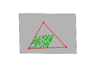
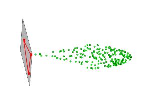
Figure 1: Panel (a): illustration of the simplex structure of $U_{\tau}$ with $K=3$, where dots denote rows of $U_{\tau}$. Panel (b): illustration of the cone structure of $U_{*}$ with $K=3$, where dots denote rows of $U_{*}$. For both panels, red dots denote pure rows and green dots represent mixed rows. For both panels, the gray plane denotes the hyperplane formed by pure rows. For the simplex structure in panel (a), all mixed rows of $U_{\tau}$ (i.e., green dots) lie in the triangle formed by the three rows of $U_{\tau}(\mathcal{I},:)$. For the cone structure in panel (b), all mixed rows of $U_{*}$ (i.e., green dots) locate at one side of the hyperplane formed by the three rows of $U_{*}(\mathcal{I},:)$. For both panels, the settings of $\Pi$ and $\Theta$ are the same as that of Experiment 1 in Section 6.3. Points in this figure have been projected and rotated from $\mathbb{R}^{3}$ to $\mathbb{R}^{2}$ for visualization.

Call the $i$-th row of $U_{\tau}$ (and $U_{*}$) a pure row if subject $i$ is pure and a mixed row otherwise. For the simplex structure of $U_{\tau}$, a pure row is one of the $K$ vertices of $U_{\tau}(\mathcal{I},:)$ and a mixed row lies inside of the simplex formed by $U_{\tau}(\mathcal{I},:)$’s $K$ rows. For the cone structure of $U_{*}$, all mixed rows locate at one side of the hyperplane formed by the $K$ rows of $U_{*}(\mathcal{I},:)$ . Figure 1 gives illustrations of the simplex structure and the cone structure when $K=3$.

Based on the two structures Ideal Simplex and Ideal Cone found in Lemma 1, we can design two spectral methods. Next, we propose the detailed construction of our methods after brief explanations of the two structures.

3.1 The GoM-SRSC algorithm

The form $U_{\tau}=\Pi U_{\tau}(\mathcal{I},:)$ is known as ideal simplex which comes from the fact that $U_{\tau}(i,:)$ is a convex linear combination of $U_{\tau}(\mathcal{I},:)$’s $K$ rows through $U_{\tau}=\Pi U_{\tau}(\mathcal{I},:)$ for $i\in[N]$. In detail, denote the simplex made by $U_{\tau}(\mathcal{I},:)$’s $K$ rows as $\mathcal{S}^{ideal}(s_{1},s_{2},\ldots,s_{K})$ with $s_{k}$ being $U_{\tau}(\mathcal{I},:)$’s $k$-th row for $k\in[K]$. We have $U_{\tau}(i,:)=\sum_{k=1}^{K}\Pi(i,k)s_{k}$, which suggests that $U_{\tau}(i,:)$ is one of the $K$ vertices of the simplex $\mathcal{S}^{ideal}(s_{1},s_{2},\ldots,s_{K})$ if subject $i$ is pure while $U_{\tau}(i,:)$ falls inside of the simplex otherwise because $\Pi\in[0,1]^{N\times K},\|\Pi(i,:)\|_{1}=1$, and $\Pi$ satisfies Condition (C1). The ideal simplex structure is also found in the SVD of $\mathscr{R}$ under GoM in [20] and the problem of estimating mixed memberships for social networks in [22, 21, 23, 24].

Since $U_{\tau}(\mathcal{I},:)$ is nonsingular, we have $\Pi=U_{\tau}U^{-1}_{\tau}(\mathcal{I},:)$, which suggests that as long as we know the index set $\mathcal{I}$, we can recover $\Pi$ using $U_{\tau}U^{-1}_{\tau}(\mathcal{I},:)$. As suggested by [25], running the successive projection (SP) algorithm [26, 27] to $U_{\tau}$’s rows can exactly return the index set $\mathcal{I}$, where SP’s detail can be found in Algorithm 1 of [27]. Set $Z=U_{\tau}U^{-1}_{\tau}(\mathcal{I},:)\equiv\Pi$, we have $\Pi(i,:)=\frac{Z(i,:)}{\|Z(i,:)\|_{1}}$ for $i\in[N]$. After recovering $\Pi$, $\Theta$ can be recovered by the 1st statement of Lemma 1. The above analysis suggests the following algorithm which we call Ideal GoM-SRSC, where SRSC is short for simplex regularized spectral clustering. Input: $\mathscr{R},K$, and $\tau\geq 0$. Output: $\Pi$ and $\Theta$.

• Compute $\mathscr{L}_{\tau}$ using Equation (3).

• Get $U\Sigma V^{\prime}$, the compact SVD of $\mathscr{L}_{\tau}$. Set $U_{\tau}=\mathscr{D}^{1/2}_{\tau}U$.

• Apply the SP algorithm to $U_{\tau}$’s rows with $K$ vertices to obtain $U_{\tau}(\mathcal{I},:)$.

• Set $Z=U_{\tau}U^{-1}_{\tau}(\mathcal{I},:)$.

• Set $\Pi(i,:)=\frac{Z(i,:)}{\|Z(i,:)\|_{1}}$ for $i\in[N]$.

• Set $\Theta=\mathscr{R}^{\prime}\Pi(\Pi^{\prime}\Pi)^{-1}$.

In practice, we only observe the response matrix $R$ and we aim at providing good estimations of $\Pi$ and $\Theta$ from $R$. To extend the ideal algorithm to the real case, first, we introduce the regularized Laplacian matrix as below:

$$L_{\tau}=D^{-1/2}_{\tau}R,$$ (4)

where $D_{\tau}=D+\tau I_{N\times N}$, and the $(i,i)$-th diagonal entry of the $N\times N$ diagonal matrix $D$ is $D(i,i)=\sum_{j=1}^{J}R(i,j)$ for $i\in[N]$. The regularized Laplacian matrix $L_{\tau}$ has been used in [13] to estimate a latent class model. By comparing Equations (3) and (4), we observe that $\mathscr{L}_{\tau}$ has a similar form as $L_{\tau}$ and it is $L_{\tau}$’s population version. Recall that $\mathscr{L}_{\tau}$ is a rank-$K$ matrix, it is expected that the top-$K$ SVD of $L_{\tau}$ satisfactorily approximates $\mathscr{L}_{\tau}$. Therefore, we let $\hat{L}_{\tau}=\hat{U}\hat{\Sigma}\hat{V}^{\prime}$ be the top-$K$ SVD of $L_{\tau}$ such that $\hat{\Sigma}=\mathrm{diag}(\sigma_{1}(L_{\tau}),\sigma_{2}(L_{\tau}),\ldots,\sigma_{K}(L_{\tau}))$, $\hat{U}=[\hat{\eta}_{1},\hat{\eta}_{2},\ldots,\hat{\eta}_{K}],\hat{V}=[\hat{\xi}_{1},\hat{\xi}_{2},\ldots,\hat{\xi}_{K}]$, $\hat{U}$ and $\hat{V}$ satisfy $\hat{U}^{\prime}\hat{U}=I_{K\times K}$ and $\hat{V}^{\prime}\hat{V}=I_{K\times K}$, where $\hat{\eta}_{k}$ and $\hat{\xi}_{k}$ denote the left and right singular vector of the $k$-th largest singular value $\hat{\sigma}_{k}(L_{\tau})$, respectively. Let $\hat{U}_{\tau}=D^{1/2}_{\tau}\hat{U}$ be an approximation of $U_{\tau}$. Then applying the SP algorithm to $\hat{U}_{\tau}$’s rows with $K$ vertices gets the estimated index set $\hat{\mathcal{I}}$, which should be a good estimation of the index set $\mathcal{I}$ when the observed response matrix $R$ is generated from the GoM model with expectation $\mathscr{R}$. Let $\hat{Z}=\mathrm{max}(0,\hat{U}_{\tau}\hat{U}^{-1}_{\tau}(\hat{\mathcal{I}},:))$ be an estimation of $Z$, where we only consider the nonnegative part of $\hat{U}_{\tau}\hat{U}^{-1}_{\tau}(\hat{\mathcal{I}},:)$ since all entries of $Z$ are nonnegative. We estimate the membership score $\Pi(i,:)$ for the $i$-th subject by using $\hat{\Pi}=\frac{\hat{Z}(i,:)}{\|\hat{Z}(i,:)\|_{1}}$ for $i\in[N]$. Finally, we estimate the item parameter matrix $\Theta$ by using $\hat{\Theta}$ calculated as $\hat{\Theta}=\mathrm{min}(M,\mathrm{max}(0,R^{\prime}\hat{\Pi}(\hat{\Pi}^{\prime}\hat{\Pi})^{-1}))$, where we truncate all entries of $R^{\prime}\hat{\Pi}(\hat{\Pi}^{\prime}\hat{\Pi})^{-1}$ to be in the range $[0,M]$ since $\Theta$’s elements are in the range $[0,M]$ theoretically. We summarize the above analysis into the following algorithm which extends the Ideal GoM-SRSC algorithm naturally to the real case with known the observed response matrix $R$.

Algorithm 1 GoM-SRSC

1:The observed response matrix $R\in\{0,1,2,\ldots,M\}^{N\times J}$, the number of latent classes $K$, and the regularization parameter $\tau$ (a good choice for $\tau$ is $M\mathrm{max}(N,J)$.).

2:The estimated membership matrix $\hat{\Pi}$ and the estimated item parameter matrix $\hat{\Theta}$.

3:Get $L_{\tau}$ by Equation (4).

4:Get $\hat{U}\hat{\Sigma}\hat{V}^{\prime}$, the top-$K$ singular value decomposition of $L_{\tau}$. Set $\hat{U}_{\tau}=D^{1/2}_{\tau}\hat{U}$.

5:Apply the SP algorithm on $\hat{U}_{\tau}$’s rows with $K$ vertices to obtain $\hat{U}_{\tau}(\hat{\mathcal{I}},:)$, where $\hat{\mathcal{I}}$ represents the estimated index set returned by SP.

6:Set $\hat{Z}=\mathrm{max}(0,\hat{U}_{\tau}\hat{U}^{-1}_{\tau}(\hat{\mathcal{I}},:))$.

7:Set $\hat{\Pi}(i,:)=\frac{\hat{Z}(i,:)}{\|\hat{Z}(i,:)\|_{1}}$ for $i\in[N]$.

8:Set $\hat{\Theta}=\mathrm{min}(M,\mathrm{max}(0,R^{\prime}\hat{\Pi}(\hat{\Pi}^{\prime}\hat{\Pi})^{-1}))$

The computational cost of our GoM-SRSC algorithm mainly comes from the top $K$ SVD of $L_{\tau}$, the SP algorithm, and the last step in estimating $\Theta$. The complexities of these three main steps are $O(\mathrm{max}(N^{2},J^{2})K),O(NK^{2})$, and $O(NJK)$, respectively. Because $K\ll\mathrm{min}(N,J)$ in this paper, as a result, our GoM-SRSC algorithm has a total complexity $O(\mathrm{max}(N^{2},J^{2})K)$.

3.2 The GoM-CRSC algorithm

$U_{*}=YU_{*}(\mathcal{I},:)$ forms a cone structure introduced in Problem 1 of [25] since the $l_{2}$ norm of $U_{*}(i,:)$ is 1 for $i\in[N]$. This form is different from the ideal simplex structure because the $N\times K$ matrix $Y$ has a different property as the membership matrix $\Pi$. Unlike the ideal simplex structure, applying the successive projection algorithm to all rows of $U_{*}$ cannot recover the $K\times K$ matrix $U_{*}(\mathcal{I},:)$. Luckily, as analyzed in [25], running the SVM-cone algorithm of [25] to all rows of $U_{*}$ can exactly recover $U_{*}(\mathcal{I},:)$ as long as $(U_{*}(\mathcal{I},:)U^{\prime}_{*}(\mathcal{I},:))^{-1}\mathbf{1}>0$ holds (here, $\mathbf{1}$ is a vector with all entries being 1) which is guaranteed by Lemma 2 below, where the SVM-cone algorithm is summarized in Algorithm 1 of [25].

Lemma 2.

Under $\mathrm{GoM}(\Pi,\Theta)$, $(U_{*}(\mathcal{I},:)U^{\prime}_{*}(\mathcal{I},:))^{-1}\mathbf{1}>0$ holds.

Therefore, we can run the SVM-cone algorithm to $U_{*}$’s rows to recover $U_{*}(\mathcal{I},:)$. Then we can recover $Y$ by setting $Y=U_{*}U^{-1}_{*}(\mathcal{I},:)$. Set $Z_{*}=UU^{-1}_{*}(\mathcal{I},:)D_{U}(\mathcal{I},\mathcal{I})\mathscr{D}^{-1/2}_{\tau}(\mathcal{I},\mathcal{I})$. The following lemma guarantees that we can recover $\Pi$ from $Z_{*}$.

Lemma 3.

Under $\mathrm{GoM}(\Pi,\Theta)$, we have $\Pi(i,:)=\frac{Z_{*}(i,:)}{\|Z_{*}(i,:)\|_{1}}$ for $i\in[N]$.

After getting $\Pi$ from $Z_{*}$ by Lemma 3, $\Theta$ can be obtained by the 1st result in Lemma 1. Then we get the Ideal GoM-CRSC algorithm below, where CRSC means cone regularized spectral clustering. Input: $\mathscr{R},K$, and $\tau\geq 0$. Output: $\Pi$ and $\Theta$.

• Compute $\mathscr{L}_{\tau}$ using Equation (3).

• Get $U\Sigma V^{\prime}$, the top-$K$ SVD of $\mathscr{L}_{\tau}$. Obtain $U_{*}$ from $U$.

• Run the SVM-cone algorithm with inputs $U_{*}$ and $K$ to obtain $U_{*}(\mathcal{I},:)$.

• Set $Z_{*}=UU^{-1}_{*}(\mathcal{I},:)D_{U}(\mathcal{I},\mathcal{I})\mathscr{D}^{-1/2}_{\tau}(\mathcal{I},\mathcal{I})$.

• Set $\Pi(i,:)=\frac{Z_{*}(i,:)}{\|Z_{*}(i,:)\|_{1}}$ for $i\in[N]$.

• Set $\Theta=\mathscr{R}^{\prime}\Pi(\Pi^{\prime}\Pi)^{-1}$.

Now, we consider the real case with known $R$ instead of its expectation $\mathscr{R}$. Let $\hat{U}_{*}=D_{\hat{U}}\hat{U}$, where $D_{\hat{U}}$ is an $N\times N$ diagonal matrix with $(i,i)$-th diagonal entry being $\frac{1}{\|\hat{U}(i,:)\|_{F}}$ for $i\in[N]$. The following algorithm extends the Ideal GoM-CRSC algorithm to the real case naturally. The computational cost of SVM-cone is $O(KN^{2})$ [28, 25]. Combing the complexity analysis of Algorithm 1, GoM-CRSC’s complexity is $O(\mathrm{max}(N^{2},J^{2})K)$.

Algorithm 2 GoM-CRSC

1:$R,K$, and $\tau$ (a good default choice for $\tau$ is $M\mathrm{max}(N,J)$.).

2:$\hat{\Pi}_{*}$ and $\hat{\Theta}_{*}$.

3:Get $L_{\tau}$ by Equation (4).

4:Get $\hat{U}\hat{\Sigma}\hat{V}^{\prime}$, the top-$K$ SVD of $L_{\tau}$. Set $\hat{U}_{*}=D_{\hat{U}}\hat{U}$.

5:Run the SVM-cone algorithm with inputs $\hat{U}_{*}$ and $K$ to obtain $\hat{U}_{*}(\hat{\mathcal{I}}_{*},:)$, where $\hat{\mathcal{I}}_{*}$ is the estimated index set returned by SVM-cone.

6:Set $\hat{Z}_{*}=\mathrm{max}(0,\hat{U}\hat{U}^{-1}_{*}(\hat{\mathcal{I}}_{*},:)D_{\hat{U}}(\hat{\mathcal{I}}_{*},\hat{\mathcal{I}}_{*})D^{-1/2}_{\tau}(\hat{\mathcal{I}}_{*},\hat{\mathcal{I}}_{*}))$.

7:Set $\hat{\Pi}_{*}(i,:)=\frac{\hat{Z}_{*}(i,:)}{\|\hat{Z}_{*}(i,:)\|_{1}}$ for $i\in[N]$.

8:Set $\hat{\Theta}_{*}=\mathrm{min}(M,\mathrm{max}(0,R^{\prime}\hat{\Pi}_{*}(\hat{\Pi}^{\prime}_{*}\hat{\Pi}_{*})^{-1}))$

4 Asymptotic consistency

Before providing the theoretical error rates of our methods, we introduce the sparsity parameter of an observed response matrix $R$. Recall that when $R\in\{0,1,2,\ldots,M\}^{N\times J}$, GoM requires $\Theta\in[0,M]^{J\times K}$, which implies that the maximum entry of $\Theta$ should be no larger than $M$. Let $\rho=\mathrm{max}_{j\in[J],k\in[K]}\Theta(j,k)$ and $B=\frac{\Theta}{\rho}$, we see that $\rho$ ranges in $[0,M]$ and $\mathrm{max}_{j\in[J],k\in[K]}B(j,k)=1$. By Equation (2) and $\mathscr{R}(i,j)=\Pi(i,:)\Theta^{\prime}(j,:)=\rho\Pi(i,:)B^{\prime}(j,:)$, we see that the probability of no-response (i.e., $R(i,j)=0$) equals $(1-\frac{\rho\Pi(i,:)B^{\prime}(j,:)}{M})^{M}$, a value decreases as $\rho$ increases, i.e., $\rho$ controls the sparsity (i.e., number of zeros) of an observed response matrix $R$. For this reason, we call $\rho$ the sparsity parameter. In real-world categorical data such as psychological test datasets and educational assessment datasets, there usually exist several subjects that do not respond to all items, i.e., there exist some no-responses for real-world categorical data. Generally speaking, the task of estimating $\Pi$ and $\Theta$ is hard when categorical data is sparse. Therefore, it is critical to investigate the performances of different methods when categorical data has different levels of sparsity. We will study $\rho$’s influence on the performance of our approaches both theoretically and numerically. Our results rely on the following sparsity assumption, which means a lower bound requirement on the sparsity parameter $\rho$ for our theoretical analysis.

Assumption 1.

$\rho\mathrm{max}(N,J)\geq M^{2}\mathrm{log}(N+J)$.

Assumption 1 is mild since it requires $\rho\geq\frac{M^{2}\mathrm{log}(N+J)}{\mathrm{max}(N,J)}$, where the lower bound is a small value when $N$ and $J$ are large. Meanwhile, it is reasonable to consider a lower bound requirement on $\rho$ since if $\rho$ is too small (i.e., there are too many zeros in $R$), it is impossible for any algorithm to have a satisfactory performance in estimating $\Pi$ and $\Theta$. We also need the following conditions to simplify our analysis.

Condition 1.

$K=O(1),J=O(N),\sigma_{K}(\Pi)=O(\sqrt{\frac{N}{K}}),\sigma_{K}(B)=O(\sqrt{\frac{J}{K}})$, and $\pi_{\mathrm{min}}=O(\frac{N}{K})$, where $\pi_{\mathrm{min}}=\mathrm{min}_{k\in[K]}\sum_{i=1}^{N}\Pi(i,k)$.

Condition 1 is also mild and this can be understood as below: $K=O(1)$ implies that $K$ is a constant number, $J=O(N)$ means that $J$ has the same order as $N$, $\sigma_{K}(\Pi)=O(\sqrt{\frac{N}{K}})$ and $\pi_{\mathrm{min}}=O(\frac{N}{K})$ means that each latent class has close size, and $\sigma_{K}(B)=O(\sqrt{\frac{J}{K}})$ means that the summation of each column of $B$ is in the same order. Let $e_{i}$ be a vector whose $i$-th element equals 1 and all the other entries are 0 in this paper. Theorem 1 below establishes the per-subject error rate in estimating $\Pi$ and the relative $l_{2}$ error in estimating $\Theta$ of our GoM-SRSC, where the error rates of our GoM-CRSC are the same as that of GoM-SRSC.

Theorem 1.

Under $\mathrm{GoM}(\Pi,\Theta)$, suppose Assumption 1 and Condition 1 hold, with high probability, we have

$$\mathrm{max}_{i\in[N]}\|e^{\prime}_{i}(\hat{\Pi}-\Pi\mathcal{P})\|_{1}=O(\sqrt{\frac{\mathrm{log}(N)}{\rho N}})\mathrm{~{}and~{}}\frac{\|\hat{\Theta}-\Theta\mathcal{P}\|_{F}}{\|\Theta\|_{F}}=O(\sqrt{\frac{\mathrm{log}(N)}{\rho N}}),$$

where $\mathcal{P}$ is a $K\times K$ permutation matrix.

We observe that the error rates decrease as the sparsity parameter $\rho$ increases according to Theorem 1, which is in line with our intuition. We also observe that the error rates decrease to zero as the number of subjects $N$ and the number of items $J$ increase to infinity, which implies the estimation consistencies of our methods. Meanwhile, by the proof of Theorem 1, $\tau\geq M\mathrm{\mathrm{missing}}{max}(N,J)$ should hold, where this requirement on $\tau$ is mainly used to simplify our theoretical bounds. In fact, we find empirically in Section 6.3 that our algorithms GoM-SRSC and GoM-CRSC are insensitive to the choice of $\tau$.

5 Quantifying the quality of latent mixed membership analysis

For real data, the true membership matrix $\Pi$ is often unknown, while an estimated membership matrix can always be obtained by applying a latent mixed membership analysis method to the observed response matrix $R$. Assuming $\hat{\Pi}_{1}$ and $\hat{\Pi}_{2}$ are the estimated membership matrices returned by two different algorithms applied to $R$ with the same number of latent classes. Since the real membership matrix $\Pi$ is unknown, it is natural to ask which algorithm returns a better partition for all subjects. This question prompts the need for a metric to assess the quality of the latent mixed membership analysis. Additionally, the number of latent classes, $K$, is usually not known for real-world categorical data, necessitating the development of a method to estimate it. In this paper, we address these two questions by providing a metric to measure the quality of the latent mixed membership analysis.

Next, we introduce our metric. Set $A=RR^{\prime}$ and call $A$ adjacency matrix. We see that $A(i,\bar{i})=R(i,:)R^{\prime}(\bar{i},:)=\sum_{j=1}^{J}R(i,j)R(\bar{i},j)$ for two distinct subjects $i$ and $\bar{i}$. To gain a better understanding of $A(i,\bar{i})$, we consider the binary response case. In this case, we see that $R(i,\bar{i})$ represents the common responses of $i$ and $\bar{i}$. Since subjects with similar memberships have similar response patterns, subjects with similar memberships should have more common responses than subjects with different memberships. This implies that $A$ can be viewed as the adjacency matrix of an assortative network in which nodes with similar memberships have more connections than nodes with different memberships [29, 30]. Our analysis suggests that applying the fuzzy modularity introduced in equation (14) of [31] to $A$ is a good choice to measure the quality of the latent mixed membership analysis. Suppose that there is an $N\times k$ estimated membership matrix $\hat{\Pi}$ returned by applying algorithm $\mathcal{M}$ to $R$ with $k$ latent classes, where $\hat{\Pi}(i,:)\geq 0$ and $\|\hat{\Pi}(i,:)\|_{1}=1$ for $i\in[N]$. The fuzzy modularity is computed in the following way:

$$Q_{\mathcal{M}}(k)=\frac{1}{\omega}\sum_{i\in[N]}\sum_{\bar{i}\in[N]}(A(i,\bar{i})-\frac{d_{i}d_{\bar{i}}}{\omega})\hat{\Pi}(i,:)\hat{\Pi}^{\prime}(\bar{i},:),$$ (5)

where $d_{i}=\sum_{j\in[N]}A(i,j)$ for $i\in[N],\omega=\sum_{i\in[N]}d_{i}$, and we denote the fuzzy modularity as $Q_{\mathcal{M}}(k)$ since it is computed using $\hat{\Pi}$, the estimated membership matrix of algorithm $\mathcal{M}$ with $k$ latent classes. When all subjects are pure, the fuzzy modularity reduces to the well-known Newman-Girvan modularity [32, 33]. For the problem of latent mixed membership analysis for real-world categorical data, larger fuzzy modularity indicates better partition and algorithms returning larger fuzzy modularity are preferred.

After defining the fuzzy modularity, we utilize the strategy proposed in [31] to determine the optimal choice of $K$ for real categorical data. Specifically, we estimate $K$ by selecting the one that maximizes the fuzzy modularity. For convenience, when we apply the latent mixed membership analysis algorithm $\mathcal{M}$ on Equation (5) to estimate $K$, we refer to this method as K$\mathcal{M}$.

6 Evaluation on synthetic categorical data

In this section, we present simulation studies. Firstly, we propose two alternative algorithms for GoM. Secondly, we introduce three evaluation metrics. Finally, we conduct thorough experimental studies.

6.1 Two alternative algorithms for fitting GoM

6.1.1 GoM-SSC

We call the first alternative method GoM-SSC, where SSC is short for simplex spectral clustering. Recall that $\mathscr{R}$’s rank is $K$ under GoM, without confusion, we let $\mathscr{R}=U\Sigma V^{\prime}$ be $\mathscr{R}$’s compact SVD such that $U^{\prime}U=I_{K\times K}$ and $V^{\prime}V=I_{K\times K}$. Since $\mathscr{R}=\Pi\Theta^{\prime}$, we have $U=\Pi\Theta^{\prime}V\Sigma^{-1}=\Pi U(\mathcal{I},:)$, where $U=\Pi U(\mathcal{I},:)$ also forms a simplex structure. Then applying the SP algorithm to $U$ returns $U(\mathcal{I},:)$. Set $Z=UU^{-1}(\mathcal{I},:)$, we have $Z\equiv\Pi$ since $U=\Pi U(\mathcal{I},:)$. The above analysis suggests the following ideal algorithm named Ideal GoM-SSC. Input: $\mathscr{R}$ and $K$. Output: $\Pi$ and $\Theta$.

• Let $U\Sigma V^{\prime}$ be $\mathscr{R}$’s top-$K$ SVD.

• Apply the SP algorithm to $U$’s rows with $K$ vertices to get $U(\mathcal{I},:)$.

• Set $Z=UU^{-1}(\mathcal{I},:)$.

• Recover $\Pi$ and $\Theta$ by the last two steps of Ideal GoM-SRSC.

Algorithm 3 below extends the Ideal GoM-SSC to the real case with known $R$ naturally.

Algorithm 3 GoM-SSC

1:$R$ and $K$.

2:$\hat{\Pi}$ and $\hat{\Theta}$.

3:Get $\hat{U}\hat{\Sigma}\hat{V}^{\prime}$, the top-$K$ SVD of $R$.

4:Apply the SP algorithm on $\hat{U}$’s rows with $K$ vertices to get $\hat{U}(\hat{\mathcal{I}},:)$.

5:$\hat{Z}=\mathrm{max}(0,\hat{U}\hat{U}^{-1}(\hat{\mathcal{I}},:))$.

6:Obtain $\hat{\Pi}$ and $\hat{\Theta}$ by steps 5 and 6 of Algorithm 1.

The computational cost of GoM-SSC is the same as our GoM-SRSC. Following a similar theoretical analysis to that of GoM-SRSC, we find that GoM-SSC’s theoretical error rates are the same as that of GoM-SRSC under Assumption 1 and Condition 1. Note that GoM-SSC differs slightly from Algorithm 2 of [20]. The slight differences are two-fold. First, similar to [21], Algorithm 2 of [20] considers an extra pruning step to reduce noise. Second, $\hat{\Theta}$ in Algorithm 2 of [20] is obtained by setting $\hat{\Theta}=\mathrm{min}(1-\epsilon,\mathrm{max}(\epsilon,\hat{V}\hat{\Sigma}\hat{U}^{\prime}\hat{\Pi}(\hat{\Pi}^{\prime}\hat{\Pi})^{-1}))$ with $\epsilon=0.001$ while $\hat{\Theta}$ is $\mathrm{min}(M,\mathrm{max}(0,R^{\prime}\hat{\Pi}(\hat{\Pi}^{\prime}\hat{\Pi})^{-1}))$ in our GoM-SSC and this difference occurs because we consider data with polytomous responses in this paper while [20] only considers data with binary responses.

6.1.2 GoM-SRM

We call the second alternative method GoM-SRM, where SRM means simplex response matrix. Recall that $\mathscr{R}=\Pi\Theta^{\prime}$ under GoM, we observe that $\mathscr{R}=\Pi\Theta^{\prime}=\Pi\mathscr{R}(\mathcal{I},:)$ naturally forms a simplex structure. Thus applying the SP algorithm to $\mathscr{R}$’s rows with $K$ vertices gets $\mathscr{R}(\mathcal{I},:)$. Note that since $\mathscr{R}(\mathcal{I},:)$ is a $K\times J$ matrix with rank $K$ (recall that $K\ll J$ in this paper), its inverse does not exist but the inverse of $\mathscr{R}(\mathcal{I},:)\mathscr{R}(\mathcal{I},:)^{\prime}$ exists. Set $Z=\mathscr{R}\mathscr{R}(\mathcal{I},:)^{\prime}(\mathscr{R}(\mathcal{I},:)\mathscr{R}^{\prime}(\mathcal{I},:))^{-1}$, we have $Z\equiv\Pi$ since $\mathscr{R}=\Pi\mathscr{R}(\mathcal{I},:)$. The following algorithm named Ideal GoM-SRM summarizes the above analysis. Input: $\mathscr{R}$ and $K$. Output: $\Pi$ and $\Theta$.

• Apply SP to $\mathscr{R}$’s rows with $K$ vertices to get $\mathscr{R}(\mathcal{I},:)$.

• Set $Z=\mathscr{R}\mathscr{R}(\mathcal{I},:)^{\prime}(\mathscr{R}(\mathcal{I},:)\mathscr{R}^{\prime}(\mathcal{I},:))^{-1}$.

• Recover $\Pi$ and $\Theta$ by the last two steps of Ideal GoM-SRSC.

The GoM-SRM algorithm below is the real case of the Ideal GoM-SRM algorithm. Compared with GoM-SRSC, GoM-CRSC, and GoM-SSC, there is no SVD step in GoM-SRM. GoM-SRM’s complexity is $O(NJK)$. Since the complexities of GoM-SRSC, GoM-CRSC, and GoM-SSC are $O(\mathrm{max}(N^{2},J^{2})K)$, GoM-SRM runs faster than the other three methods when $N\neq J$.

Algorithm 4 GoM-SRM

1:$R$ and $K$.

2:$\hat{\Pi}$ and $\hat{\Theta}$.

3:Apply SP algorithm to $R$’s rows with $K$ vertices to get $R(\hat{\mathcal{I}},:)$.

4:$\hat{Z}=\mathrm{max}(0,RR(\hat{\mathcal{I}},:)^{\prime}(R(\hat{\mathcal{I}},:)R^{\prime}(\hat{\mathcal{I}},:))^{-1})$.

5:Obtain $\hat{\Pi}$ and $\hat{\Theta}$ by steps 5 and 6 of Algorithm 1.

6.2 Evaluation metrics

In our simulation studies, we assess the performance of our algorithms in accurately estimating the membership matrix $\Pi$, the item parameter matrix $\Theta$, and the number of latent classes $K$ using three metrics below. For the estimation of $\Pi$ in simulated categorical data with known $\Pi$, we calculate the Hamming error, defined as the minimum over all $K\times K$ permutation matrices $\mathcal{P}$ of the relative $\ell_{1}$ norm difference between $\hat{\Pi}$ and $\Pi\mathcal{P}$, i.e., $\mathrm{min}_{\mathcal{P}\in\mathcal{S}}\frac{1}{N}\|\hat{\Pi}-\Pi\mathcal{P}\|_{1}$, where $\mathcal{S}$ denotes the set collecting all $K\times K$ permutation matrices. This metric, ranging between 0 and 1, quantifies the discrepancy between $\Pi$ and its estimation $\hat{\Pi}$ with smaller values indicating better estimation accuracy.

For the estimation of $\Theta$, we utilize the Relative error, which is defined as the minimum over all $K\times K$ permutation matrices $\mathcal{P}$ of the relative Frobenius norm difference between $\hat{\Theta}$ and $\Theta\mathcal{P}$, i.e., $\mathrm{min}_{\mathcal{P}\in\mathcal{S}}\frac{\|\hat{\Theta}-\Theta\mathcal{P}\|_{F}}{\|\Theta\|_{F}}$. This metric measures the discrepancy between $\Theta$ and its estimation $\hat{\Theta}$ with smaller values indicating better estimation accuracy.

Finally, to measure the performance of algorithms in inferring $K$, we calculate the accuracy rate, defined as the fraction of times an algorithm correctly identifies $K$ out of a total number of independent trials. This metric, ranging between 0 and 1, quantifies the success rate of algorithms in estimating $K$ with larger values indicating higher accuracy. By using these three metrics, we can objectively evaluate the performance of our proposed algorithms in estimating $\Pi$, $\Theta$, and $K$ in a controlled simulation environment.

6.3 Simulations

We test the effectiveness and accuracies of our methods by investigating their sensitivities to the regularization parameter $\tau$, the sparsity parameter $\rho$, and the number of subjects $N$ in this part. Unless specified, for all simulations, we set $J=\frac{N}{4},K=3$, and $M=4$ (i.e., $R(i,j)\in\{0,1,2,3,4\}$ for $i\in[N],j\in[J]$). Let each latent class have $N_{0}$ pure subjects. Let the top $3N_{0}$ subjects $\{1,2,\ldots,N_{0}\}$ be pure and the rest $(N-3N_{0})$ subjects be mixed. For mixed subject $i$, we set its membership score $\Pi(i,:)$ as $\Pi(i,:)=(r_{1},r_{2},1-r_{1}-r_{2})$, where $r_{1}=\frac{\mathrm{rand}(1)}{2}$, $r_{1}=\frac{\mathrm{rand}(1)}{2}$, and $\mathrm{rand}(1)$ is a random number generated from a Uniform distribution on $[0,1]$. Let $N_{0}=\frac{N}{4}$ in all simulations. Set $\bar{B}$ as an $J\times K$ matrix such that its $(j,k)$-th entry is $\mathrm{rand}(1)$. Set $B=\frac{\bar{B}}{\mathrm{max}_{j\in[J],k\in[K]}\bar{B}(j,k)}$ (in this way, $B$’s maximum entry is 1). Except for the case where we study the choice of $\tau$, we set $\tau$ as its default value $M\mathrm{max}(N,J)$. $\rho$ and $N$ are set independently for each experiment. For each parameter setting, we report the averaged metric over 100 repetitions.

(a) Hamming error against $\tau$

(b) Relative error against $\tau$

(c) Running time against $\tau$

(d) Accuracy against $\tau$

Figure 2: Results of Experiment 1.

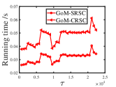
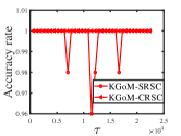
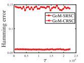
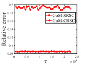
Experiment 1: Changing $\tau$. Recall that there is a regularization parameter $\tau$ in our algorithms GoM-SRSC and GoM-CRSC, in this experiment, we investigate the effect of $\tau$ empirically. We set $(\rho,N)=(1,800)$ and $\tau=\alpha M\mathrm{max}(N,J)$. We vary $\alpha$ in the range $\{0.2,0.4,\ldots,7\}$. The results, displayed in Figure 2, indicate that (1) our GoM-SRSC and GoM-CRSC are insensitive to the choice of the regularizer $\tau$. In this paper we choose the default value of $\tau$ as $M\mathrm{max}(N,J)$ because it matches our theoretical analysis and our methods are insensitive to $\tau$; (2) GoM-CRSC returns more accurate estimations of $\Pi$ and $\Theta$ than GoM-SRSC; (3) GoM-SRSC runs slightly faster than GoM-CRSC; (4) Our KGoM-SRSC and KGoM-CRSC have high accuracies in estimating $K$, indicating the effectiveness of our metric computed by Equation (5) in measuring the quality of latent mixed membership analysis.

(a) Hamming error against $\rho$

(b) Relative error against $\rho$

(c) Running time against $\rho$

(d) Accuracy against $\rho$

Figure 3: Results of Experiment 2.

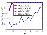
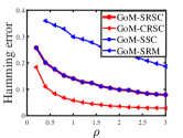
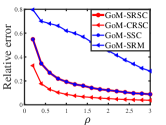
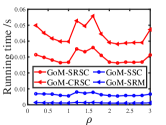
Experiment 2: Changing $\rho$. Here, we investigate the sensitivity of our methods to the sparsity parameter $\rho$. Let $N=800$ and $\rho$ range in $\{0.2,0.4,\ldots,3\}$. Results are shown in Figure 3. We have the following conclusions: (1) as we expect, our methods have better performances in estimating $\Pi$ and $\Theta$ as $\rho$ increases, and this verifies our analysis after Theorem 1; (2) for the task of estimating $\Pi$ and $\Theta$, GoM-CRSC outperforms the other three methods, GoM-SRSC enjoys similar performances as GoM-SSC, and GoM-SRM performs poorest. For computing time, GoM-SRM runs fastest and this supports our computational cost analysis for GoM-SRM; (3) for the task of inferring $K$, our KGoM-SRSC, KGoM-CRSC, and KGoM-SSC enjoy high accuracies while KGoM-SRM performs poorest. Again, the high accuracy of KGoM-SRSC, KGoM-CRSC, and KGoM-SSC guarantees the high effectiveness of our metric in quantitating the strength of latent mixed membership analysis.

(a) Hamming error against $N$

(b) Relative error against $N$

(c) Running time against $N$

(d) Accuracy against $N$

Figure 4: Results of Experiment 3.

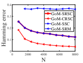
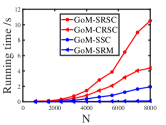
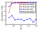
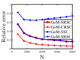
Experiment 3: Changing $N$. Let $\rho=0.2$ and $N$ take values from the set $\{800,1600,\ldots,8000\}$. Figure 4 shows the results. We see that (1) GoM-SRSC, GoM-CRSC, and GoM-SCC behave better as $N$ and $J$ increase, which verifies our analysis after Theorem 1; (2) GoM-CRSC has the best performances in estimating $\Pi$ and $\Theta$ though GoM-CRSC runs slowest; (3) GoM-SRSC performs similarly to GoM-SCC and GoM-SRM performs poorest; (4) Our methods process categorical data with 8000 subjects and 2000 items within 12 seconds; (5) Our KGoM-SRSC, KGoM-CRSC, and KGoM-SSC enjoy satisfactory performances in estimate $K$, indicating the powerfulness of our metric.

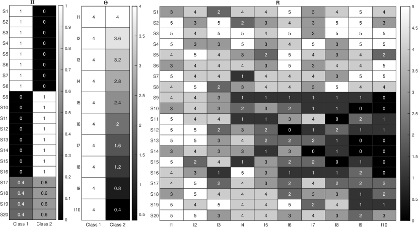
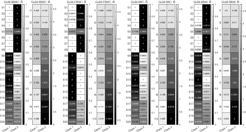
Experiment 4: A toy example. Set $K=2,N=20,J=10$, and $M=5$. Set $\Pi$ and $\Theta$ as the 1st and 2nd matrices in Figure 5, respectively. The last matrix of Figure 5 displays a response matrix $R$ generated from the GoM model under the above setting. We apply our algorithms to this $R$ and Table 1 records the numerical results. We see that our GoM-CRSC performs best in estimating $\Pi$ and $\Theta$, GoM-SRSC outperforms GoM-SCC slightly, and all methods estimate $K$ correctly for this toy example. Meanwhile, applying our methods to the $R$ in the last matrix of Figure 5 gets the estimations of $\Pi$ and $\Theta$, and we show these estimations in Figure 6. As we expect, since the Hamming error and Relative error are non-zero for all methods by Table 1, $\hat{\Pi}$ (and $\hat{\Theta}$) differs slightly from $\Pi$ (and $\Theta$) for each method. We also find that estimating the memberships for mixed subjects is more challenging than that of pure subjects for all methods. Finally, as suggested by our theoretical analysis after Theorem 1 and numerical analysis for Experiment 3, to make the estimations more accurate, we should increase $N$ and $J$. However, we set $N=20$ and $J=10$ for this experiment mainly for the visualizations of $\Pi,\Theta,R,\hat{\Pi},$ and $\hat{\Theta}$.

Figure 5: We set $\Pi$ and $\Theta$ for Experiment 4 as the 1st and 2nd matrices, respectively. The 3rd matrix shows a $R$ generated from the GoM model in Experiment 4. Here, S$i$ denotes subject $i$ and I$j$ means item $j$.

Figure 6: Estimated $\Pi$ and $\Theta$ of each method for Experiment 4. Here, S$i$ denotes subject $i$ and I$j$ means item $j$.

Table 1: Results of Experiment 4.

	Hamming error	Relative error	Estimated $K$
GoM-SRSC	0.0650	0.1142	2
GoM-CRSC	0.0529	0.1034	2
GoM-SCC	0.0654	0.1146	2
GoM-SRM	0.0772	0.1251	2

7 Application to real-world categorical data

We apply our methods to real categorical data in this part. Table 2 summarizes basic information for real categorical data considered in this paper, where $\varsigma=\frac{\mathrm{Number~{}of~{}zero~{}elements~{}of~{}}R}{NJ}$ denotes the proportion of no-responses in $R$ and we have removed those subjects that have no response to all items for all data. The true mixed memberships and number of latent classes are unknown for all real data used here. These datasets can be downloaded from http://konect.cc/networks/movielens-100k_rating/ and https://openpsychometrics.org/_rawdata/.

For MovieLens 100k, users rate movies and a higher rating score means more likes. For IPIP, 1=Strongly disagree, 2=Disagree, 3=Neither agree nor disagree, 4=Agree, and 5=Strongly agree. For KIMS, 1=Never or very rarely true, 2=Rarely true, 3=Sometimes true, 4=Often true, and 5=Very often or always true. For NPI, 1 means one choice of a question and 2 means another choice. For all data, 0 means no response. Details of all statements for IPIP, KIMS, and NPI can be found in Figures 8, 9, and 10, respectively.

By Table 2, we see that the MovieLens 100k data is the sparsest while there are only a few no-responses for the other three datasets. This can be understood in the following way. Because MovieLens 100k is a user-rating-movie network and the number of users is smaller than that of movies, a user usually rates just a few movies. For comparison, because the other three datasets are test data and the number of individuals is much larger than that of questions, an individual usually answers all questions and only a few individuals have no responses to some questions.

To determine how many latent classes one should use for each data, we run our algorithms to $R$ to compute the modularity by Equation (5). Based on the results reported in Table 3, we observe that (1) our GoM-CRSC always returns the largest modularity for all data, which suggests that the estimated number of latent classes for MovieLens 100k, IPIP, KIMS, and NPI should be 3, 2, 2, and 2, respectively; (2) GoM-SRSC performs similarly to GoM-SSC; (3) GoM-SRM returns poorest partitions of latent mixed memberships since its modularity is the smallest for each data. These observations are consistent with our numerical findings in Experiments 2-4. From now on, we only consider our GoM-CRSC for real data analysis since its modularity is the largest for each data.

Table 2: Basic information of real-world categorical data used in this paper.

	Subject meaning	Item meaning	$N$	$J$	$M$	$\varsigma$
MovieLens 100k	User	Movie	943	1682	5	93.7%
International Personality Item Pool (IPIP) personality test	Individual	Statement	1004	40	5	0.6%
Kentucky Inventory of Mindfulness Skills (KIMS) test	Individual	Statement	601	39	5	0.59%
Narcissistic Personality Inventory (NPI) test	Individual	Question	11241	40	2	0.3%

Table 3: The $K$ maximizing the modularity and the respective modularity of each method for data in Table 2.

Dataset	GoM-SRSC	GoM-CRSC	GoM-SSC	GoM-SRM
MovieLens 100k	(2, 0.0461)	(3, 0.0730)	(2, 0.0501)	(2,0176)
IPIP	(4, 0.0021)	(2, 0.0067)	(4, 0.0021)	(4,0.0019)
KIMS	(3, 0.0027)	(2, 0.0081)	(3, 0.0027)	(3, 0.0024)
NPI	(4, 0.0017)	(2, 0.0054)	(4, 0.0017)	(14, 0.00028)

Let $\hat{\Pi}$ and $\hat{\Theta}$ be the estimated membership matrix and the estimated item parameter matrix returned by applying GoM-CRSC to real data with $K$ latent classes, where $K$ is the one returned by KGoM-CRSC. To simplify our analysis, we name the $K$ latent classes as Class 1, Class 2, $\ldots$, and Class $K$ for each data.

Definition 1.

Call subject $i$ a highly pure subject if $\mathrm{max}_{k\in[K]}\hat{\Pi}(i,k)\geq 0.9$ and a highly mixed subject if $\mathrm{max}_{k\in[K]}\hat{\Pi}(i,k)\leq 0.7$ for $i\in[N]$. Define $\mu=\frac{|\{i\in[N]:\mathrm{max}_{k\in[K]}\hat{\Pi}(i,k)\geq 0.9\}|}{N}$ and $\nu=\frac{|\{i\in[N]:\mathrm{max}_{k\in[K]}\hat{\Pi}(i,k)\leq 0.7\}|}{N}$.

Definition 1 says that $\mu$ ($\nu$) is the proportion of highly pure (mixed) subjects. Results reported in Table 4 show that though most subjects are highly pure, there still exist many highly mixed subjects for each data. By Table 4, we see that GoM-CRSC processes data with 11241 subjects and 40 items within 2 seconds, which suggests its efficiency.

Recall that $\mathscr{R}=\Pi\Theta^{\prime}$ under GoM, we have $\mathscr{R}(i,j)=\sum_{k\in[K]}\Pi(i,k)\Theta(j,k)$, which suggests that a larger $\Theta(j,k)$ gives a larger $\mathscr{R}(i,j)$ given the membership score $\Pi(i,:)$ of subject $i$, i.e., a larger $\Theta(j,k)$ tends to make $R(i,j)$ larger since $\mathscr{R}(i,j)$ is the expectation of $R(i,j)$ under GoM. Based on this observation, next, we interpret the estimated latent classes for each data briefly.

Table 4: $\mu,\nu$, and runtime when applying GoM-CRSC to real data considered in this paper.

dataset	$\mu$	$\nu$	Runtime
MovieLens 100k	0.4602	0.2333	0.1077s
IPIP	0.6036	0.2112	0.0467s
KIMS	0.6040	0.1947	0.0345s
NPI	0.6249	0.1882	1.5903s

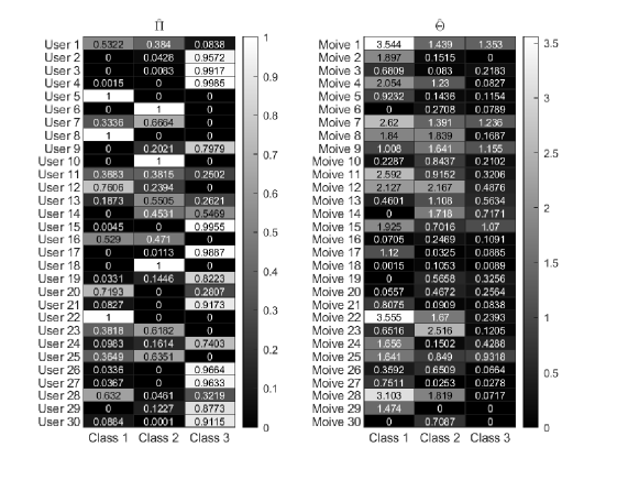
For MovieLens 100k, Figure 7 displays a subset of $\hat{\Pi}$ and a subset of $\hat{\Theta}$ for better visualization. From the estimated mixed memberships of subjects $2,3,4,15,17,21,26,27$, and 30, we see that these subjects are highly pure and they are more likely to belong to Class 3. Meanwhile, subjects 12, 20, and 28 are more likely to belong to Class 1. From the right matrix of Figure 7, we find that $\hat{\Theta}(j,1)$ is usually larger than $\hat{\Theta}(j,2)$ while $\hat{\Theta}(j,2)$ is usually larger than $\hat{\Theta}(j,3)$ for $j\in[30]$. In fact, we have $\sum_{j\in[1682]}\hat{\Theta}(j,1)=704.6280,\sum_{j\in[1682]}\hat{\Theta}(j,2)=552.2857$, and $\sum_{j\in[1682]}\hat{\Theta}(j,3)=178.6997$. Based on the above observation, Class 1 can be interpreted as users with an optimistic view of movies, Class 2 can be interpreted as users with a neutral view of movies, and Class 3 can be interpreted as users with a passive view of movies. Users in Class 1 are more likely to give higher ratings to movies than users in Class 2 and Class 3.

Figure 7: Left matrix: heatmap of the estimated mixed memberships of the first 30 users for the MovieLens 100k data. Right matrix: heatmap of the estimated item parameters of the first 30 items for the MovieLens 100k data.

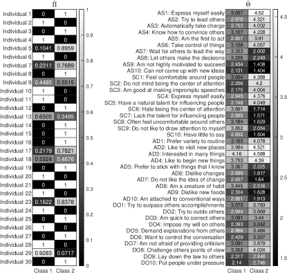
Figure 8: Left matrix: the estimated mixed memberships of the first 30 individuals for the IPIP data. Right matrix: heatmap of $\hat{\Theta}$ for the IPIP data, where AS, SC, AD, and DO mean four personality factors assertiveness, social confidence, adventurousness, and dominance, respectively.

For IPIP, the estimated mixed memberships of the first 30 individuals and the estimated item parameter matrix $\hat{\Theta}$ are displayed in Figure 8. From $\hat{\Pi}$, we can find subjects’ memberships. Recall that for the IPIP data, a higher response value to a statement means a stronger agreement, by analyzing $\hat{\Theta}$, we interpret Class 1 as people who are socially passive and Class 2 as socially optimistic. People in Class 2 are usually more assertive, adventurous, and dominant than those in Class 1.

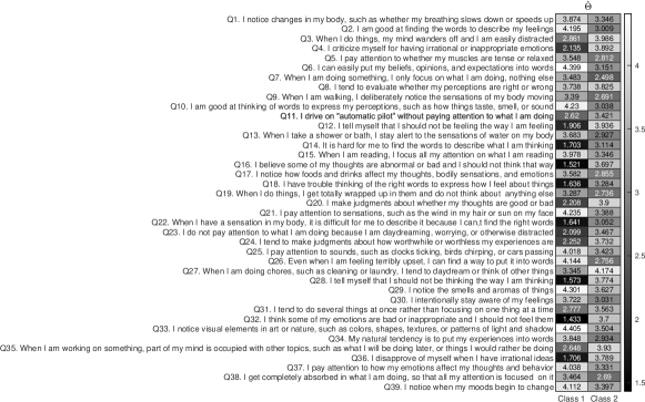
Figure 9: Heatmap of $\hat{\Theta}$ for the KIMS data.

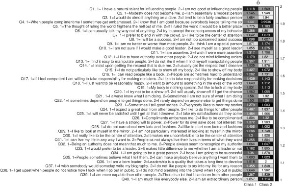
Figure 10: Heatmap of $\hat{\Theta}$ for the NPI data.

For KIMS, Figure 9 shows $\hat{\Theta}$’s heatmap. For this data, we interpret Class 1 as people who are mindful and Class 2 as people who are mindless. People in Class 1 are more focused on himself/herself than those in Class 2.

Figure 10 displays $\hat{\Theta}$’s heatmap for the NPI data. For this data, Class 1 can be interpreted as people who are narcissistic and Class 2 as people who are modest. People in Class 1 are more narcissistic than those in Class 2.

8 Conclusion

In this paper, we present two new efficient regularized spectral clustering algorithms for mixed membership estimation and item parameter estimation under the Grade of Membership model for categorical data. We obtain theoretical per-subject error rates for mixed membership estimation and show that the two algorithms yield consistent parameter estimations under a mild condition on data sparsity. To measure the quality of the latent mixed membership analysis in categorical data, we propose a metric that computes the fuzzy modularity based on the product of the response matrix and its transpose. We estimate $K$ for categorical data generated from the GoM model by combining our metric with our algorithms. Substantial experimental results demonstrate the effectiveness and accuracies of our algorithms in estimating the mixed membership matrix, the item parameter matrix, and the number of latent classes under GoM. In particular, our methods for estimating $K$ enjoy high accuracies and this supports the usefulness of our metric in evaluating the quality of the latent mixed membership analysis. Our work contributes to a more comprehensive understanding of mixed membership estimation and item parameter estimation under the GoM model for categorical data. The proposed algorithms and metric offer valuable tools for analyzing categorical data and evaluating the quality of latent mixed membership analysis, and we hope that they will have wide applications in latent class analysis, enabling researchers to better understand structures of categorical data and extract meaningful insights.

CRediT authorship contribution statement

Huan Qing is the sole author of this article.

Declaration of competing interest

The author declares no competing interests.

Data availability

Data and code will be made available on request.

Appendix A Proofs under GoM

A.1 Proof of Lemma 1

Proof.

For the 1st statement, $\mathscr{R}=\Pi\Theta^{\prime}\rightarrow\mathscr{R}^{\prime}=\Theta\Pi^{\prime}\rightarrow\mathscr{R}^{\prime}\Pi=\Theta\Pi^{\prime}\Pi\rightarrow\Theta=\mathscr{R}^{\prime}\Pi(\Pi^{\prime}\Pi)^{-1}$, where the $K\times K$ matrix $\Pi^{\prime}\Pi$ is nonsingular since $\Pi$’s rank is $K$ when Condition (C1) hold.

For the 2nd statement, $\mathscr{L}_{\tau}=\mathscr{D}^{-1/2}_{\tau}\mathscr{R}=\mathscr{D}^{-1/2}_{\tau}\Pi\Theta^{\prime}=U\Sigma V^{\prime}$ under GoM gives $U_{\tau}=\mathscr{D}^{1/2}_{\tau}U=\Pi\Theta^{\prime}V\Sigma^{-1}$. By $\Pi(\mathcal{I},:)=I_{K\times K}$, we have $U_{\tau}(\mathcal{I},:)=\Pi(\mathcal{I},:)\Theta^{\prime}V\Sigma^{-1}=\Theta^{\prime}V\Sigma^{-1}$, i.e., $U_{\tau}=\Pi U_{\tau}(\mathcal{I},:)$. Sure, when $\Pi(i,:)=\Pi(\bar{i},:)$ for two distinct subjects $i$ and $\bar{i}$, we get $U_{\tau}(i,:)=U_{\tau}(\bar{i},:)$.

For the 3rd statement, since $U=\mathscr{D}^{-1/2}_{\tau}\Pi\Theta^{\prime}V\Sigma^{-1}$, we have $U(i,:)=\mathscr{D}^{-1/2}_{\tau}(i,i)\Pi(i,:)\Theta^{\prime}V\Sigma^{-1}$, which gives that $U_{*}(i,:)=\frac{\Pi(i,:)\Theta^{\prime}V\Sigma^{-1}}{\|\Pi(i,:)\Theta^{\prime}V\Sigma^{-1}\|_{F}}=\frac{\Pi(i,:)U_{\tau}(\mathcal{I},:)}{\|\Pi(i,:)U_{\tau}(\mathcal{I},:)\|_{F}}=\frac{\Pi(i,:)\mathscr{D}^{1/2}_{\tau}(\mathcal{I},\mathcal{I})U(\mathcal{I},:)}{\|\Pi(i,:)U_{\tau}(\mathcal{I},:)\|_{F}}=\frac{\Pi(i,:)\mathscr{D}^{1/2}_{\tau}(\mathcal{I},\mathcal{I})D^{-1}_{U}(\mathcal{I},\mathcal{I})D_{U}(\mathcal{I},\mathcal{I})U(\mathcal{I},:)}{\|\Pi(i,:)U_{\tau}(\mathcal{I},:)\|_{F}}=\frac{\Pi(i,:)\mathscr{D}^{1/2}_{\tau}(\mathcal{I},\mathcal{I})D^{-1}_{U}(\mathcal{I},\mathcal{I})U_{*}(\mathcal{I},:)}{\|\Pi(i,:)U_{\tau}(\mathcal{I},:)\|_{F}}$ for $i\in[N]$. Sure, when $\Pi(i,:)=\Pi(\bar{i},:)$, we have $U_{*}(i,:)=U_{*}(\bar{i},:)$. ∎

A.2 Proof of Lemma 2

Proof.

By the proof of Lemma 1, we know that $U=\mathscr{D}^{-1/2}_{\tau}\Pi U_{\tau}(\mathcal{I},:)=\mathscr{D}^{-1/2}_{\tau}\Pi\mathscr{D}^{1/2}_{\tau}(\mathcal{I},\mathcal{I})U(\mathcal{I},:)$. By $I_{K\times K}=U^{\prime}U$, we have $(U(\mathcal{I},:)U^{\prime}(\mathcal{I},:))^{-1}=\mathscr{D}^{1/2}_{\tau}(\mathcal{I},\mathcal{I})\Pi^{\prime}\mathscr{D}^{-1}_{\tau}\Pi\mathscr{D}^{1/2}_{\tau}(\mathcal{I},\mathcal{I})$. Then we have $(U_{*}(\mathcal{I},:)U^{\prime}_{*}(\mathcal{I},:))^{-1}=(N_{U}(\mathcal{I},\mathcal{I})U(\mathcal{I},:)U^{\prime}(\mathcal{I},:)N_{U}(\mathcal{I},\mathcal{I}))^{-1}=N^{-1}_{U}(\mathcal{I},\mathcal{I})\mathscr{D}^{1/2}_{\tau}(\mathcal{I},\mathcal{I})\Pi^{\prime}\mathscr{D}^{-1}_{\tau}\Pi\mathscr{D}^{1/2}_{\tau}(\mathcal{I},\mathcal{I})N^{-1}_{U}(\mathcal{I},\mathcal{I})$. Since all entries of $N_{U},\mathscr{D}_{\tau}$, and $\Pi$ are nonnegative, we have $(U_{*}(\mathcal{I},:)U^{\prime}_{*}(\mathcal{I},:))^{-1}\mathbf{1}>0$. ∎

A.3 Proof of Lemma 3

Proof.

Since $Y=D_{o}\Pi\mathscr{D}^{1/2}_{\tau}(\mathcal{I},\mathcal{I})D^{-1}_{U}(\mathcal{I},\mathcal{I})$ by Lemma 1, we have $D_{o}\Pi=YD_{U}(\mathcal{I},\mathcal{I})\mathscr{D}^{-1/2}_{\tau}(\mathcal{I},\mathcal{I})=U_{*}U^{-1}_{*}(\mathcal{I},:)D_{U}(\mathcal{I},\mathcal{I})\mathscr{D}^{-1/2}_{\tau}(\mathcal{I},\mathcal{I})=D_{U}UU^{-1}_{*}(\mathcal{I},:)D_{U}(\mathcal{I},\mathcal{I})\mathscr{D}^{-1/2}_{\tau}(\mathcal{I},\mathcal{I})$, which gives that $D^{-1}_{U}D_{0}\Pi=UU^{-1}_{*}(\mathcal{I},:)D_{U}(\mathcal{I},\mathcal{I})\mathscr{D}^{-1/2}_{\tau}(\mathcal{I},\mathcal{I})\equiv Z_{*}$. Because $D^{-1}_{U}D_{0}$ is a diagonal matrix, we have $\Pi(i,:)=\frac{Z_{*}(i,:)}{\|Z_{*}(i,:)\|_{1}}$ for $i\in[N]$. ∎

A.4 Proof of Theorem 1

Proof.

Let $\lambda_{k}(X)$ denote the $k$-th largest eigenvalue in magnitude , $\kappa(X)$ denote the conditional number, $\|X\|$ denote the spectral norm, and $\|X\|_{2\rightarrow\infty}$ denote the maximum $l_{2}$-norm among all rows for any matrix $X$ in this paper. Set $\delta_{\mathrm{min}}=\mathrm{min}_{i\in[N]}\mathscr{D}(i,i)$ and $\delta_{\mathrm{max}}=\mathrm{max}_{i\in[N]}\mathscr{D}(i,i)$. To prove this theorem, we need Lemma 4 and Lemma 5 below.

Lemma 4.

Under $\mathrm{GoM}(\Pi,\Theta)$, we have below results:

• $\sqrt{\frac{\tau+\delta_{\mathrm{min}}}{\tau+\delta_{\mathrm{max}}}}\frac{1}{\sqrt{K\lambda_{1}(\Pi^{\prime}\Pi)}}\leq\|U(i,:)\|_{F}\leq\sqrt{\frac{\tau+\delta_{\mathrm{max}}}{\tau+\delta_{\mathrm{min}}}}\frac{1}{\sqrt{\lambda_{K}(\Pi^{\prime}\Pi)}}\mathrm{~{}for~{}}i\in[N]$.

• $\frac{\tau+\delta_{\mathrm{min}}}{\lambda_{1}(\Pi^{\prime}\Pi)}\leq\lambda_{K}(U_{\tau}(\mathcal{I},:)U^{\prime}_{\tau}(\mathcal{I},:))\leq\lambda_{1}(U_{\tau}(\mathcal{I},:)U^{\prime}_{\tau}(\mathcal{I},:))\leq\frac{\tau+\delta_{\mathrm{max}}}{\lambda_{K}(\Pi^{\prime}\Pi)}$.

• $\frac{\tau+\delta_{\mathrm{min}}}{(\tau+\delta_{\mathrm{max}})\kappa(\Pi^{\prime}\Pi)}\leq\lambda_{K}(U_{*}(\mathcal{I},:)U^{\prime}_{*}(\mathcal{I},:))\leq\lambda_{1}(U_{*}(\mathcal{I},:)U^{\prime}_{*}(\mathcal{I},:))\leq K\frac{\tau+\delta_{\mathrm{max}}}{\tau+\delta_{\mathrm{min}}}\kappa(\Pi^{\prime}\Pi)$.

• $\frac{\rho^{2}\lambda_{K}(\Pi^{\prime}\Pi)\lambda_{K}(B^{\prime}B)}{\tau+\delta_{\mathrm{max}}}\leq\lambda_{K}(\mathscr{L}_{\tau}\mathscr{L}^{\prime}_{\tau})\leq\lambda_{1}(\mathscr{L}_{\tau}\mathscr{L}^{\prime}_{\tau})\leq\frac{\rho^{2}\lambda_{1}(\Pi^{\prime}\Pi)\lambda_{1}(B^{\prime}B)}{\tau+\delta_{\mathrm{min}}}$.

• $\|V(j,:)\|_{F}\leq\frac{K^{1.5}\kappa(\Pi)}{\sigma_{K}(B)}\sqrt{\frac{\tau+\delta_{\mathrm{max}}}{\tau+\delta_{\mathrm{min}}}}$ for $j\in[J]$.

Proof.

The first three bullets are guaranteed by Lemmas C.2 and C.3 of [34]. For the fourth statement, since $\mathscr{L}_{\tau}=\mathscr{D}^{-1/2}_{\tau}\mathscr{R}=\mathscr{D}^{-1/2}_{\tau}\Pi\Theta^{\prime}=\rho\mathscr{D}^{-1/2}_{\tau}\Pi B^{\prime}$, we have

$$\lambda_{K}(\mathscr{L}_{\tau}\mathscr{L}^{\prime}_{\tau})=\rho^{2}\lambda_{K}(\mathscr{D}^{-1/2}_{\tau}\Pi B^{\prime}B\Pi^{\prime}\mathscr{D}^{-1/2}_{\tau})=\rho^{2}\lambda_{K}(\mathscr{D}^{-1}_{\tau}\Pi B^{\prime}B\Pi^{\prime})\geq\rho^{2}\lambda_{K}(\mathscr{D}^{-1}_{\tau})\lambda_{K}(\Pi B^{\prime}B\Pi^{\prime})\geq\frac{\rho^{2}\lambda_{K}(\Pi^{\prime}\Pi)\lambda_{K}(B^{\prime}B)}{\tau+\delta_{\mathrm{max}}},$$

and

$$\lambda_{1}(\mathscr{L}_{\tau}\mathscr{L}^{\prime}_{\tau})=\rho^{2}\lambda_{1}(\mathscr{D}^{-1/2}_{\tau}\Pi B^{\prime}B\Pi^{\prime}\mathscr{D}^{-1/2}_{\tau})=\rho^{2}\lambda_{1}(\mathscr{D}^{-1}_{\tau}\Pi B^{\prime}B\Pi^{\prime})\leq\rho^{2}\lambda_{1}(\mathscr{D}^{-1}_{\tau})\lambda_{1}(\Pi B^{\prime}B\Pi^{\prime})\leq\frac{\rho^{2}\lambda_{1}(\Pi^{\prime}\Pi)\lambda_{1}(B^{\prime}B)}{\tau+\delta_{\mathrm{min}}}.$$

For the last statement, since $\mathscr{L}_{\tau}=\mathscr{D}^{-1/2}_{\tau}\mathscr{R}=\mathscr{D}^{-1/2}_{\tau}\Pi\Theta^{\prime}=\rho\mathscr{D}^{-1/2}_{\tau}\Pi B^{\prime}=U\Sigma V^{\prime}$, we have $V=\rho B\Pi^{\prime}\mathscr{D}^{-1/2}_{\tau}U\Sigma^{-1}$, which gives that

$$\|V(j,:)\|_{F} =\rho\|B(j,:)\Pi^{\prime}\mathscr{D}^{-1/2}_{\tau}U\Sigma^{-1}\|_{F}\leq\rho\|B(j,:)\|_{F}\|\Pi^{\prime}\mathscr{D}^{-1/2}_{\tau}U\|_{F}\|\Sigma^{-1}\|_{F}\leq\rho\sqrt{K}\|\Pi^{\prime}\mathscr{D}^{-1/2}_{\tau}\|_{F}\|\Sigma^{-1}\|_{F}$$

$$\leq\frac{\rho K\|\mathscr{D}^{-1/2}_{\tau}\Pi\|_{F}}{\sigma_{K}(\mathscr{L}_{\tau})}\leq\frac{\rho K\|\Pi\|_{F}}{\sigma_{K}(\mathscr{L}_{\tau})\sqrt{\tau+\delta_{\mathrm{min}}}}\leq\frac{\rho K^{1.5}\|\Pi\|}{\sigma_{K}(\mathscr{L}_{\tau})\sqrt{\tau+\delta_{\mathrm{min}}}}\leq\frac{K^{1.5}\kappa(\Pi)}{\sigma_{K}(B)}\sqrt{\frac{\tau+\delta_{\mathrm{max}}}{\tau+\delta_{\mathrm{min}}}},$$

where the last inequality holds by the 4th statement of this lemme. ∎

Lemma 5.

Under $\mathrm{GoM}(\Pi,\Theta)$, suppose that Assumption 1 and Condition 1 are satisfied, and $\sigma_{K}(\mathscr{L}_{\tau})\gg\sqrt{\frac{\rho N\mathrm{log}(N)}{\tau}}$. With high probability, we have

$$\varpi:=\|\hat{U}\hat{U}^{\prime}-UU^{\prime}\|_{2\rightarrow\infty}=O(\sqrt{\frac{\mathrm{log}(N+J)}{\rho NJ}}).$$

Proof.

Set $H=\hat{U}^{\prime}U$. Let $H=U_{H}\Sigma_{H}V^{\prime}_{H}$ be $H$’s top-$K$ SVD. Set $\mathrm{sgn}(H)=U_{H}V^{\prime}_{H}$. Under $\mathrm{GoM}(\Pi,\Theta)$, for $i\in[N],j\in[J]$, we get $\mathbb{E}(R(i,j)-\mathscr{R}(i,j))=0$, $\mathbb{E}((L_{\tau}(i,j)-\mathscr{L}_{\tau}(i,j))^{2})=\mathbb{E}[(\frac{R(i,j)}{\sqrt{\tau+D(i,i)}}-\frac{\mathscr{R}(i,j)}{\sqrt{\tau+\mathscr{D}(i,i)}})^{2}]\leq\frac{\mathrm{Var}(R(i,j))}{\mathrm{min}(\tau+1,\tau+\delta_{\mathrm{min}})}=\frac{M\frac{\mathscr{R}(i,j)}{M}(1-\frac{\mathscr{R}(i,j)}{M})}{\mathrm{min}(\tau+1,\tau+\delta_{\mathrm{min}})}=\frac{\mathscr{R}(i,j)(1-\frac{\mathscr{R}(i,j)}{M})}{\mathrm{min}(\tau+1,\tau+\delta_{\mathrm{min}})}\leq\frac{\rho}{\mathrm{min}(\tau+1,\tau+\delta_{\mathrm{min}})}=O(\rho/\tau),|L_{\tau}(i,j)-\mathscr{L}_{\tau}(i,j)|\leq\frac{M}{\sqrt{\mathrm{min}(\tau+1,\tau+\delta_{\mathrm{min}})}}=O(M/\sqrt{\tau})$. Meanwhile, since $0<\delta_{\mathrm{min}}\leq\delta_{\mathrm{max}}=\mathrm{max}_{i\in[N]}\sum_{j=1}^{J}\mathscr{R}(i,j)=\rho\mathrm{max}_{i\in[N]}\sum_{j=1}^{J}\Pi(i,:)B^{\prime}(j,:)\leq\rho J\leq\rho\mathrm{max}(N,J)\leq M\mathrm{max}(N,J)$ and $\frac{\tau+\delta_{\mathrm{max}}}{\tau+\delta_{\mathrm{min}}}$ approximates to 1 as $\tau$ increases, we see that to make $\frac{\tau+\delta_{\mathrm{max}}}{\tau+\delta_{\mathrm{min}}}$ close to 1, a larger $\tau$ is preferred. Suppose that $\tau\geq M\mathrm{max}(N,J)$, we have $\frac{\tau+\delta_{\mathrm{max}}}{\tau+\delta_{\mathrm{min}}}=O(1)$ though $\delta_{\mathrm{max}}\geq\delta_{\mathrm{min}}$. Then, by Lemma 4, Condition 1, and $\tau\geq M\mathrm{max}(N,J)$, we have $\mu=\mathrm{max}(\frac{N\|U\|^{2}_{2\rightarrow\infty}}{K},\frac{J\|V\|^{2}_{2\rightarrow\infty}}{K})=O(\frac{\tau+\delta_{\mathrm{max}}}{\tau+\delta_{\mathrm{min}}})=O(1)$ and $\kappa(\mathscr{L}_{\tau})=O(1)$. When Assumption 1 is satisfied, we get $c_{b}=\frac{O(M/\sqrt{t})}{\sqrt{\frac{\rho}{\tau}\frac{\mathrm{max}(N,J)}{\mu\mathrm{log}(N+J)}}}\leq O(1)$. Therefore, when $\sigma_{K}(\mathscr{L}_{\tau})\gg\sqrt{\frac{\rho N\mathrm{log}(N)}{\tau}}$ is satisfied, according to Theorem 4 of [35], with high probability, we have

$$\|\hat{U}\mathrm{sgn}(H)-U\|_{2\rightarrow\infty}\leq O(\frac{\sqrt{K\rho\mathrm{log}(N+J)}}{\sigma_{K}(\mathscr{L}_{\tau})\sqrt{\tau}}).$$

By Lemma 4, we have $\|\hat{U}\mathrm{sgn}(H)-U\|_{2\rightarrow\infty}=O(\frac{1}{\sigma_{K}(\Pi)\sigma_{K}(B)}\sqrt{\frac{K\mathrm{log}(N+J)}{\rho}})$. $\hat{U}^{\prime}\hat{U}=I_{K\times K}$ and $U^{\prime}U=I_{K\times K}$ give $\|\hat{U}\hat{U}^{\prime}-UU^{\prime}\|_{2\rightarrow\infty}\leq 2\|U-\hat{U}\mathrm{sgn}(H)\|_{2\rightarrow\infty}$. Hence, by Condition 1, we get

$$\|\hat{U}\hat{U}^{\prime}-UU^{\prime}\|_{2\rightarrow\infty}=O(\frac{1}{\sigma_{K}(\Pi)\sigma_{K}(B)}\sqrt{\frac{K\mathrm{log}(N+J)}{\rho}})=O(\sqrt{\frac{\mathrm{log}(N+J)}{\rho NJ}}).$$

∎

For GoM-SRSC, its per-subject error rates of memberships equal that of community detection for mixed networks. Therefore, by the proof of Theorem 1 in [34], there exist two $K$-by-$K$ permutation matrices $\mathcal{P}$ and $\mathcal{P}_{*}$ such that with high probability,

$$\mathrm{max}_{i\in[N]}\|e^{\prime}_{i}(\hat{\Pi}-\Pi\mathcal{P})\|_{1}=O(K^{1.5}\varpi\kappa(\Pi)\sqrt{\lambda_{1}(\Pi^{\prime}\Pi)})\mathrm{~{}and~{}}\mathrm{max}_{i\in[N]}\|e^{\prime}_{i}(\hat{\Pi}_{*}-\Pi\mathcal{P}_{*})\|_{1}=O(\frac{K^{6.5}\varpi\kappa^{4.5}(\Pi)\lambda_{1}^{1.5}(\Pi^{\prime}\Pi)}{\pi_{\mathrm{min}}}),$$

where we have used the fact that $\frac{\tau+\delta_{\mathrm{max}}}{\tau+\delta_{\mathrm{min}}}=O(1)$ when $\tau\geq M\mathrm{max}(N,J)$ since $\delta_{\mathrm{min}}\leq\delta_{\mathrm{max}}\leq M\mathrm{max}(N,J)$. Then by Condition 1 and Lemma 5, we get

$$\mathrm{max}_{i\in[N]}\|e^{\prime}_{i}(\hat{\Pi}-\Pi\mathcal{P})\|_{1}=O(\sqrt{\frac{\mathrm{log}(N)}{\rho N}})\mathrm{~{}and~{}}\mathrm{max}_{i\in[N]}\|e^{\prime}_{i}(\hat{\Pi}_{*}-\Pi\mathcal{P}_{*})\|_{1}=O(\sqrt{\frac{\mathrm{log}(N)}{\rho N}}).$$

Next, we bound $\|\hat{\Theta}-\Theta\mathcal{P}\|$. Because $R^{\prime}\hat{\Pi}(\hat{\Pi}^{\prime}\hat{\Pi})^{-1}$ is usually almost the same as $\hat{\Theta}$, we use the bound of $\|R^{\prime}\hat{\Pi}(\hat{\Pi}^{\prime}\hat{\Pi})^{-1}-\Theta\mathcal{P}\|$ as that of $\|\hat{\Theta}-\Theta\mathcal{P}\|$.

$$\|R^{\prime}\hat{\Pi}(\hat{\Pi}^{\prime}\hat{\Pi})^{-1}-\Theta\mathcal{P}\|=\|R^{\prime}\hat{\Pi}(\hat{\Pi}^{\prime}\hat{\Pi})^{-1}-\mathscr{R}^{\prime}\Pi(\Pi^{\prime}\Pi)^{-1}\mathcal{P}\|\leq\|(R^{\prime}-\mathscr{R}^{\prime})\hat{\Pi}(\hat{\Pi}^{\prime}\hat{\Pi})^{-1}\|+\|\mathscr{R}^{\prime}(\hat{\Pi}(\hat{\Pi}^{\prime}\hat{\Pi})^{-1}-\Pi(\Pi^{\prime}\Pi)^{-1}\mathcal{P})\|$$

$$\leq\|R-\mathscr{R}\|\|\hat{\Pi}(\hat{\Pi}^{\prime}\hat{\Pi})^{-1}\|+\|\mathscr{R}\|\hat{\Pi}(\hat{\Pi}^{\prime}\hat{\Pi})^{-1}-\Pi(\Pi^{\prime}\Pi)^{-1}\mathcal{P}\|\leq\frac{\|R-\mathscr{R}\|}{\sigma_{K}(\hat{\Pi})}+\rho\sigma_{1}(\Pi)\sigma_{1}(B)\|\hat{\Pi}(\hat{\Pi}^{\prime}\hat{\Pi})^{-1}-\Pi(\Pi^{\prime}\Pi)^{-1}\mathcal{P}\|$$

$$=O(\frac{\|R-\mathscr{R}\|}{\sigma_{K}(\Pi)})+\rho\sigma_{1}(\Pi)\sigma_{1}(B)\|\hat{\Pi}(\hat{\Pi}^{\prime}\hat{\Pi})^{-1}-\Pi(\Pi^{\prime}\Pi)^{-1}\mathcal{P}\|,$$ (6)

where we use $\sigma_{K}(\Pi)$ to approximate $\sigma_{K}(\hat{\Pi})$ because $\hat{\Pi}$ is a good approximation of $\Pi$. By the proof of Theorem 1 [13], we know that when Assumption 1 holds, with high probability, we have $\|R-\mathscr{R}\|=O(\sqrt{\rho\mathrm{max}(N,J)\mathrm{log}(N+J)})$, which gives that

$$\|R^{\prime}\hat{\Pi}(\hat{\Pi}^{\prime}\hat{\Pi})^{-1}-\Theta\mathcal{P}\|_{F}\leq\sqrt{K}\|R^{\prime}\hat{\Pi}(\hat{\Pi}^{\prime}\hat{\Pi})^{-1}-\Theta\mathcal{P}\|=O(\frac{\sqrt{\rho K\mathrm{max}(N,J)\mathrm{log}(N+J)}}{\sigma_{K}(\Pi)}).$$

Because $\|\Theta\|_{F}=\rho\|B\|_{F}\geq\rho\sigma_{1}(B)$, we obtain

$$\frac{\|R^{\prime}\hat{\Pi}(\hat{\Pi}^{\prime}\hat{\Pi})^{-1}-\Theta\mathcal{P}\|_{F}}{\|\Theta\|_{F}}=O(\sqrt{\frac{K\mathrm{max}(N,J)\mathrm{log}(N+J)}{\rho\sigma^{2}_{K}(\Pi)\sigma^{2}_{1}(B)}}).$$

By Condition 1, we have

$$\frac{\|\hat{\Theta}-\Theta\mathcal{P}\|_{F}}{\|\Theta\|_{F}}=O(\sqrt{\frac{\mathrm{log}(N)}{\rho N}}).$$

Similarly, we have $\frac{\|\hat{\Theta}_{*}-\Theta\mathcal{P}_{*}\|_{F}}{\|\Theta\|_{F}}=O(\sqrt{\frac{\mathrm{log}(N)}{\rho N}})$. ∎

References

• [1] D. Sloane, S. P. Morgan, An introduction to categorical data analysis, Annual review of sociology 22 (1) (1996) 351–375.
• [2] A. Agresti, Categorical data analysis, Vol. 792, John Wiley & Sons, 2012.
• [3] J. Kunegis, Konect: the koblenz network collection, in: Proceedings of the 22nd international conference on world wide web, 2013, pp. 1343–1350.
• [4] L. A. Goodman, Exploratory latent structure analysis using both identifiable and unidentifiable models, Biometrika 61 (2) (1974) 215–231.
• [5] E. S. Garrett, S. L. Zeger, Latent class model diagnosis, Biometrics 56 (4) (2000) 1055–1067.
• [6] T. Asparouhov, B. Muthén, Using Bayesian priors for more flexible latent class analysis, in: proceedings of the 2011 joint statistical meeting, Miami Beach, FL, American Statistical Association Alexandria, VA, 2011.
• [7] A. White, T. B. Murphy, BayesLCA: An R package for Bayesian latent class analysis, Journal of Statistical Software 61 (2014) 1–28.
• [8] Y. Li, J. Lord-Bessen, M. Shiyko, R. Loeb, Bayesian latent class analysis tutorial, Multivariate behavioral research 53 (3) (2018) 430–451.
• [9] Z. Bakk, J. K. Vermunt, Robustness of stepwise latent class modeling with continuous distal outcomes, Structural equation modeling: a multidisciplinary journal 23 (1) (2016) 20–31.
• [10] H. Chen, L. Han, A. Lim, Beyond the em algorithm: constrained optimization methods for latent class model, Communications in Statistics-Simulation and Computation 51 (9) (2022) 5222–5244.
• [11] Y. Gu, G. Xu, A joint mle approach to large-scale structured latent attribute analysis, Journal of the American Statistical Association 118 (541) (2023) 746–760.
• [12] Z. Zeng, Y. Gu, G. Xu, A Tensor-EM Method for Large-Scale Latent Class Analysis with Binary Responses, Psychometrika 88 (2) (2023) 580–612.
• [13] H. Qing, Latent class analysis by regularized spectral clustering, arXiv preprint arXiv:2310.18727.
• [14] M. A. Woodbury, J. Clive, A. Garson Jr, Mathematical typology: a grade of membership technique for obtaining disease definition, Computers and biomedical research 11 (3) (1978) 277–298.
• [15] E. A. Erosheva, Grade of membership and latent structure models with application to disability survey data, Ph.D. thesis, Carnegie Mellon University (2002).
• [16] E. A. Erosheva, S. E. Fienberg, C. Joutard, Describing disability through individual-level mixture models for multivariate binary data, The annals of applied statistics 1 (2) (2007) 346.
• [17] I. C. Gormley, T. B. Murphy, A grade of membership model for rank data, Bayesian Analysis 4 (2) (2009) 265 – 295.
• [18] Y. Gu, E. A. Erosheva, G. Xu, D. B. Dunson, Dimension-grouped mixed membership models for multivariate categorical data, Journal of Machine Learning Research 24 (88) (2023) 1–49.
• [19] A. Robitzsch, sirt: Supplementary Item Response Theory Models, r package version 3.13-194 (2023).
URL https://CRAN.R-project.org/package=sirt
• [20] L. Chen, Y. Gu, A spectral method for identifiable grade of membership analysis with binary responses, arXiv preprint arXiv:2305.03149.
• [21] X. Mao, P. Sarkar, D. Chakrabarti, Estimating mixed memberships with sharp eigenvector deviations, Journal of the American Statistical Association 116 (536) (2021) 1928–1940.
• [22] M. Panov, K. Slavnov, R. Ushakov, Consistent estimation of mixed memberships with successive projections, in: Complex Networks & Their Applications VI: Proceedings of Complex Networks 2017 (The Sixth International Conference on Complex Networks and Their Applications), Springer, 2018, pp. 53–64.
• [23] J. Jin, Z. T. Ke, S. Luo, Mixed membership estimation for social networks, Journal of Econometrics.
• [24] H. Qing, J. Wang, Bipartite mixed membership distribution-free model. a novel model for community detection in overlapping bipartite weighted networks, Expert Systems with Applications 235 (2024) 121088.
• [25] X. Mao, P. Sarkar, D. Chakrabarti, Overlapping clustering models, and one (class) svm to bind them all, Advances in Neural Information Processing Systems 31.
• [26] M. C. U. Araújo, T. C. B. Saldanha, R. K. H. Galvao, T. Yoneyama, H. C. Chame, V. Visani, The successive projections algorithm for variable selection in spectroscopic multicomponent analysis, Chemometrics and intelligent laboratory systems 57 (2) (2001) 65–73.
• [27] N. Gillis, S. A. Vavasis, Semidefinite programming based preconditioning for more robust near-separable nonnegative matrix factorization, SIAM Journal on Optimization 25 (1) (2015) 677–698.
• [28] C.-C. Chang, C.-J. Lin, Libsvm: a library for support vector machines, ACM transactions on intelligent systems and technology (TIST) 2 (3) (2011) 1–27.
• [29] M. E. Newman, Assortative mixing in networks, Physical review letters 89 (20) (2002) 208701.
• [30] M. E. Newman, Mixing patterns in networks, Physical review E 67 (2) (2003) 026126.
• [31] T. Nepusz, A. Petróczi, L. Négyessy, F. Bazsó, Fuzzy communities and the concept of bridgeness in complex networks, Physical Review E 77 (1) (2008) 016107.
• [32] M. E. Newman, M. Girvan, Finding and evaluating community structure in networks, Physical review E 69 (2) (2004) 026113.
• [33] M. E. Newman, Modularity and community structure in networks, Proceedings of the national academy of sciences 103 (23) (2006) 8577–8582.
• [34] H. Qing, J. Wang, Regularized spectral clustering under the mixed membership stochasticblock model, Neurocomputing (2023) 126490.
• [35] Y. Chen, Y. Chi, J. Fan, C. Ma, et al., Spectral methods for data science: A statistical perspective, Foundations and Trends® in Machine Learning 14 (5) (2021) 566–806.