Learn2extend: Extending sequences by retaining their statistical properties with mixture models
Abstract
This paper addresses the challenge of extending general finite sequences of real numbers within a subinterval of the real line, maintaining their inherent statistical properties by employing machine learning. Our focus lies on preserving the gap distribution and pair correlation function of these point sets. Leveraging advancements in deep learning applied to point processes, this paper explores the use of an auto-regressive Sequence Extension Mixture Model (SEMM) for extending finite sequences, by estimating directly the conditional density, instead of the intensity function. We perform comparative experiments on multiple types of point processes, including Poisson, locally attractive, and locally repelling sequences, and we perform a case study on the prediction of Riemann function zeroes. The results indicate that the proposed mixture model outperforms traditional neural network architectures in sequence extension with the retention of statistical properties. Given this motivation, we showcase the capabilities of a mixture model to extend sequences, maintaining specific statistical properties, i.e. the gap distribution, and pair correlation indicators.
Keywords: Point Processes, Pair Correlation, Mixture Models
1 Introduction
1.1 Problem formulation
Point processes (Cox & Isham, 2018; Daley & Vere-Jones, 2003) play a central role in modern mathematics as they are often used in mathematical models of real world phenomena Babu & Feigelson (1996); Snyder & Miller (1991); Mohler et al. (2011). However, depending on the particular type of point process, it can be expensive to generate instances of point processes, or to extend given point samples Beutler & Leneman (1966); Perman et al. (1992). The main aim of this paper is to investigate how to extend a given finite sequence of real numbers contained in a subinterval of the real line so that basic statistical properties of this point set are maintained.
Problem 1
Given a sequence of points in a subset of the real line, extend this sequence such that the pair correlation function as well as the gap distributions are maintained.
If we view the input as an instance of a random process, then this is an extremely hard statistical problem, i.e., we try to infer an underlying model from a single sample. The main point of our work is to leverage deep learning to approximate a sequence extension model.
1.2 Motivation and previous work
Modeling point processes has been a long-standing problem, that is ubiquitous in multiple real-world domains, ranging from physics Fox (1978), neuroscience Johnson (1996), and epidemiology Gatrell et al. (1996) to telecommunication networks Haenggi (2017), and social networks Wasserman (1980). Moving beyond standard statistics practices Stoyan (2006), machine learning advancements have started to be more imminent into the realm of modeling of point processes Li et al. (2018); Urschel et al. (2017); Mei & Eisner (2017); Zuo et al. (2020). A key element of multiple machine learning approaches is the estimation of the conditional intensity function (e.g. Poisson processes Du et al. (2016); Omi et al. (2019), and Hawkes processes Zuo et al. (2020)). Although estimating intensity function has proven to be effective, and efficient in numerous cases (i.e. when the likelihood estimation is tractable), in this work, and following the advancements of Shchur et al. (2020), we estimate directly the conditional density using mixture models, targeting flexibility to multiple types of sequences.
Going one step further than the sequence extension with retention of statistical properties, we are interested on how such a model can perform in a multiple next-terms prediction of well-studied sequences. Motivation for this question comes from recent advances on the prediction of the zeros of the Riemann function on the critical line; see Vartziotis & Merger (2018); Kampe & Vysogorets (2018); Chen et al. (2021); Shanker (2012; 2019; 2022). The authors in Kampe & Vysogorets (2018) developed a machine learning model based on neural networks to predict the next zero of the Riemann zeta function, based on a set of previous zeros. This work has two interesting aspects. First, the authors mostly used distances between neighboring zeros as input features in their models. Second, this work exploits the existence of the Riemann Siegel function, which is, in a way, an underlying real-valued function that governs the location of the zeros. Hence, given the Universal Approximation Theorem for neural networks it is not too surprising that this approach worked reasonably well. The network basically learns the underlying function and bases its predictions on that. However, what can be done if such an underlying function does not exist or is not known?
The pair correlation conjecture of Montgomery Montgomery (1972); Odlyzko (1987; 1992); Vartziotis & Merger (2018) predicts a very particular pair correlation structure of the sequence of zeta zeros. Hence, the neural network to predict the location of zeros, is therefore also able to extend a given sequence so that its pair correlation strucutre is maintained. Motivated by the fact that this neural network bases its predictions on information about distances of consecutive points, we were led to wonder whether we can train a machine learning model that can extend an arbitrary sequence so that its pair correlation structure is maintained - however, without the knowledge or use of an underlying function. In other words, whether using only one of the two ingredients used for the prediction of zeta zeros is sufficient to extend arbitrary sequences so that statistical properties are maintained. This question naturally requires a different approach as we can not rely on evaluations of an underlying real-valued, continuous function governing the locations of the points as input parameters.
1.3 Results
In this study, we explore the application of mixture models to predict the subsequent terms of sequences while preserving certain statistical indicators. Specifically, our emphasis lies on preserving the gap distribution and the pair correlation function of the extended sequences. To demonstrate the model’s generalizability, we evaluated its performance on various classes of sequences: Poisson sequences, locally attractive sequences, and the eigenvalues of the circular unit ensemble.
Our results indicate that the mixture model adeptly extends these sequences, effectively conserving their inherent statistical properties. In comparison to basic neural network architectures designed for multi-step next-term prediction, our auto-regressive mixture model, which samples future sequence terms in batches, exhibits superior performance both in the prediction of terms and in the retention of gap distribution and pair correlation function. Furthermore, we assess the model’s inference capabilities through a case study focused on extending the zeroes of the function. Our findings reveal that the predicted values closely align with the actual values, with no evident error propagation.
1.4 Outlook
In Section 2 we introduce the statistical descriptors we use as well as the different types of point processes we are interested in. Section 3 contains a first approach to the extension of point processes, that is the rejection sampling, which illustrates the main challenges we face. We address these challenges in Section 4 suggesting an ML-based mixture model, that estimates the conditional density Section 5 contains experimental results showing the strength of the proposed models in the retention of the statistical properties of extended sequences. Finally, we conclude this paper in Section 6.
2 Preliminaries
2.1 Point processes
To define point processes, as well as their statistical indicators, we follow Girotti (2022). Given an arbitrary collection, , of points on the real line, we say that a configuration is a subset of that locally contains a finite number of points, i.e. for every bounded interval . A locally finite point process on is a probability measure on the space of all configurations of points . If is a probability function on with respect to the Lebesgue measure which is invariant under permutations of the variables, then defines a point process. The mapping
which assigns to a Borel set the expected number of points in , is a measure on . Assuming there exists a density wrt the Lebesgue measure, i.e., the 1-point correlation function, we have
in which represents the probability to have a point in the infinitesimal interval . Furthermore, the two-point correlation function (if it exists) is a function of 2 variables such that for distinct points
is the probability to have a point in each infinitesimal interval , .
2.2 Poissonian pair correlations
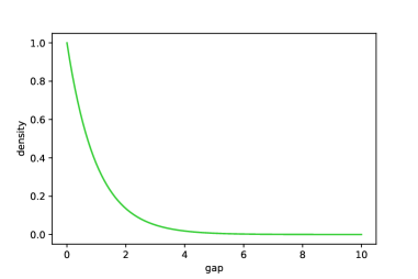
For a Poisson process the number of points in a given set has a Poisson distribution. Moreover, the number of points in disjoint sets are stochastically independent. A homogeneous Poisson process of rate is a Poisson process on with intensity measure in which is the Lebesgue measure on . In our one-dimensional setting, the rate of the Poisson process can be interpreted as the expected number of points in a unit interval. Hence, the number of points in any interval of length is a Poisson random variable with parameter . There is an important characterisation of homogeneous Poisson point processes in terms of its inter-point distances (or gaps), , with . The so-called Interval Theorem (Last & Penrose, 2018, Theorem 7.2) shows that a point process on is Poissonian with rate if and only if its gaps , for are independent and exponentially distributed with parameter . Moreover, it is shown (Last & Penrose, 2018, Eample 8.10) that the two-point correlation function of a stationary Poisson process is given by the constant function .
2.3 Determinantal point processes
We follow Girotti (2022). A point process with correlation functions is determinantal if there exists a kernel such that for every and every we have
The kernel is called correlation kernel of the determinantal point process. The particular structure of a determinantal point process allows to compute the gap probabilities. We refer to (Girotti, 2022, Section 3) for the general process and to the next subsection for a particular example.
2.4 Circular unitary ensemble (CUE)
In 1963 Dyson derived the two-point correlation function for the eigenvalues of unitary matrices. Therefore, let be an unitary matrix; i.e. . Denote the eigenvalues of by , where and . We write
| (1) |
for the normalized (unfolded) eigenphases (Note that is considered modulo , but not !). We define
We use the Haar measure, denoted as , (the natural invariant measure) on to define
in which is taken uniformly wrt the Haar measure. Then Dyson proved Dyson (1962) that the limit distribution
exists and takes the form
where is Dirac’s -function and
2.5 Empirical gap distributions and pair correlations
We give an empirical introduction to gap distributions and pair correlations which is closely related to our algorithmic approach. Let be an infinite sequence of points on the positive real line which is normalised so that . Let
which measures correlations between pairs of points. If there exists a limit distribution, , for , i.e.,
then
in which is the two-point correlation function – note that is written as a function of the distance between two points, instead of a function of a pair of points.
Moreover, we define to be the -th gap between consecutive points of the sequence. It follows from our assumption that the have mean 1 and we define
with
and (if the limit distribution exists)
2.6 Montgomery’s pair correlation conjecture
Using the Riemann-Siegel -function and the Riemann-Siegel -function allows for the computation of huge amounts of zeros of the Riemann zeta function; see for example Odlyzko (1992). These large scale computations can also enable the effective numerical investigation of various famous conjectures surrounding the zeros. Montgomery Montgomery (1972) formulated the following conjecture about the pair correlation of the normalised zeros of the Riemann zeta function:
Conjecture 1
For fixed ,
as .
Furthermore, the Gaussian Unitary Ensemble (GUE) hypothesis asserts that the zeroes of the Riemann zeta function are distributed (at microscopic and mesoscopic scales) like the eigenvalues of a GUE random matrix, and which generalises the pair correlation conjecture regarding pairs of such zeroes. An analogous hypothesis has also been made for other -functions; see Katz & Sarnak (1999); Rudnick & Sarnak (1996). Importantly, this also suggests a distribution for the gaps of normalised zeros of the zeta function.
3 Rejection sampling
To further illustrate our problem, we first discuss a basic approach to the extension of sequences in the following, and, in particular, explain why this approach does not work in general.
Importantly, the Poisson point process can be characterised by its gap distribution. The so-called Interval Theorem (Last & Penrose, 2018, Theorem 7.2) shows that a point process on is Poissonian with rate if and only if its gaps , for are independent and exponentially distributed with parameter . Moreover, it is known (Last & Penrose, 2018, Example 8.10) that the two-point correlation function of a stationary Poisson process is given by the constant function ; see Figure 1.

While the Poisson point process is characterised via its gap distribution function, a similar result does not exist for eigenvalues of the CUE or GUE. In fact, given that the sequences of eigenvalues can be described as a determinantal point process, it is possible to derive the two-point correlation function of these processes and in turn to find the gap distributions. However, there are no theorems that establish the other direction, i.e., start from a gap distribution and derive the two-point correlation function.
Based on this lack of theoretical results, our first experimental question is whether in our concrete practical situations gap distributions can be utilised to extend sequences, i.e.,
Question 1
Are gap distributions sufficient to extend a given point sample such that its pair correlation function is maintained?
In other words, can we find a, possibly heuristic, algorithm based on the empirical gap distributions of an input sequence to build an extension that preserves the pair correlation function of the input?
3.1 Empirical Study
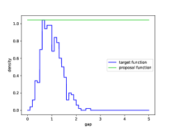
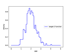
We use the finite input to determine a discrete approximation to the gap distribution of the sequence and use this approximation (rescaled to a PDF) in the form of a histogram target function to extend our point-set using classical rejection sampling.
To be more formal, given a set of points in , i.e.,
such that for all and for all , we seek to extend this sequence such that the resulting sequence
has the same (up to a small pointwise error) pair correlation function as the initial sequence. Our algorithm can be described as follows:
-
1.
Compute the empirical gap distribution and pair correlations for the sorted input sequence.
-
2.
Use a histogram approximation of the empirical gap distribution to extend the input sequence via rejection sampling.
-
3.
Calculate and output the empirical gap distribution and empirical pair correlation histogram of the extended sequence considering new terms only.
Experiment 1: Poisson Process
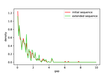
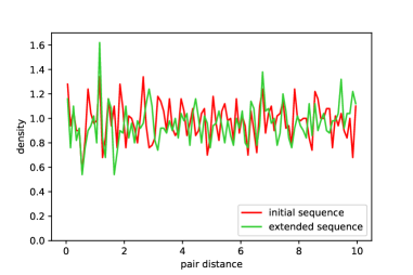
As a sanity check, we first extend sequences of points coming from a homogeneous Poisson point process. In Figure 2 we show a comparison between the empirical gap distribution (left) and the empirical pair correlation function (right) of one input sequence (red) and its extension (green). Overall, and not surprisingly, the algorithm is successful at extending a Poisson sequence to maintaining the gap distribution and pair correlation structure.
Experiment 2: Extension of sequence of eigenvalues of CUE
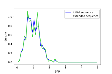
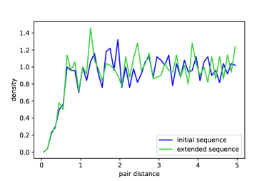
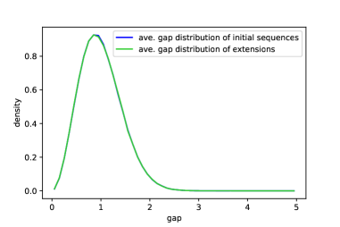
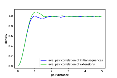
In our second experiment, we extend sequences of normalised eigenphases (see equation equation 1) of unitary matrices from the CUE ensemble. Figure 3 shows a comparison between the empirical gap distribution (left) and the empirical pair correlation function (right) of a single input sequence (blue) and its extension from rejection sampling (green). In Figure 4 we compare the average gap distribution and average pair correlation function of 1000 such sequences from the CUE ensemble with those of their extensions (new points only considered). Again, we see the algorithm is successful at replicating the gap distribution of input sequences in their extensions.
However, in Figure 4 (right) we see that the average pair correlation of the extended sequences is certainly not a perfect match, with a clear bump present around . Hence, this clearly shows that the gap distribution is in general not sufficient to determine the exact pair correlation.
3.2 Discussion
In Experiment 2 we observe a bump at around 1 in the graph of the pair correlation function of the extended sequences that is not present in the input. The immediate conclusion is that we seem to have the approximately right list of gaps, but their order is not correct. In other words, it seems that our local-to-global extension does not work in the case of eigenvalues of the CUE.
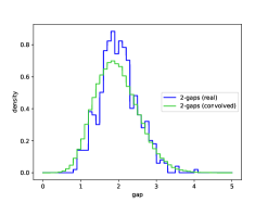
To explore this phenomenon further, we look at the 2-gaps of the input and extension. Note that it can be shown that the distribution of the sum of two independent random variables looks like the convolution of the distribution functions.
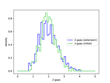
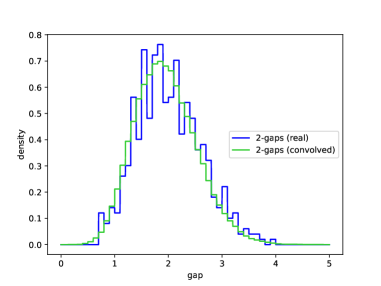
We observe that our input sequences have a 2-gap distribution different from the convolution of its gap distribution with itself; see Figure 5. However, we also observe that the extensions have a 2-gap distribution similar to the convolution of its gap distribution; see Figure 6. Hence, the problem with using our extension procedure in Experiment 2 is the assumption that gaps are independent while, in reality, there is a dependence corresponding to the local repulsion behavior of the underlying point process.
4 Learning point processes
Machine learning models have emerged as versatile tools for understanding and predicting point processes Kulesza & Taskar (2012); Mariet & Sra (2015); Zuo et al. (2020). By employing algorithms that can recognize intricate patterns within large volumes of data, these models can encapsulate the underlying dynamics of sequential events in both time and space.
For instance, in the area of social media, predicting the times at which users post or engage can be modeled as a point process Monti et al. (2019); Ahmad et al. (2020), and ML can help discern the factors that drive user activity peaks or decreases. Another compelling application is in finance, especially high-frequency trading Paiva et al. (2019). The timing of trades, often triggered by a myriad of factors including news releases, market sentiments, or algorithmic strategies, can be seen as a point process. Machine learning models can be used to predict the likelihood of trading events within minuscule time frames, offering traders insights into immediate future market activities.
4.1 Learning with Mixture distributions
Moving beyond clustering applications Celeux et al. (2018), we can apply mixture models to estimate the conditional density of point processes, and more particularly of temporal point processes, as noted by Shchur et al. (2020). Consider a general finite sequence , In this context, modeling the individual terms of the sequence is parallel to modeling the event times in a temporal point process. The primary focus in this analogy shifts to the modeling of the gaps between successive terms in the point process, denoted as . These gaps, known as inter-event times in the realm of temporal point processes, represent the intervals between consecutive events. Following (Shchur et al., 2020)’s work, and due to the fact that the sequence gaps of our interest are positive, we employ log-normal distributions as mixture components. For a number of mixture components, the probability density function of a log-normal mixture can be defined as:
| (2) |
where are the mixture weights, and are the standard statistical measures (i.e. mean, and standard deviation).
Sampling from mixture models typically involves two steps: i) Component Selection, where a component from the mixture is sampled using a categorical distribution based on the mixing weights, and ii) Data Generation, where once a component is selected, a data point from the chosen component’s distribution is sampled. This two-step process can written in closed form as following:
| (3) | ||||
| (4) | ||||
| (5) |
The samples drawn using the procedure above are differentiable (Jang et al., 2017) through the Gumbel-softmax trick with respect to the means and scales . This sampling procedure yields samples that are differentiable, as noted by Shchur et al. (2020) through the application of the Gumbel-softmax technique Jang et al. (2017). This differentiability is crucial, particularly with respect to the parameters of interest, and , enabling efficient gradient-based optimization methods.
4.2 Sequence Extension Mixture Model
In Section 4.1, we have shown how we can sample from mixture models, given the parameters of the distribution . Now, we proceed by describing how we can obtain these parameters through the lens of recursive neural networks, and consequently defining the Sequence Extension Mixture Model (SEMM), following the derivations from Shchur et al. (2020).
Context vectors
Given a sequence of point process terms , we define the context vector for each time step of the sequence, that is dependent on all the previous sequence terms: For this modeling, we make use of a recurrent neural network (RNN) that embeds a sequence of terms into a fixed-size vector . Specifically, we utilize a multi-layer gated recurrent unit (GRU) Cho et al. (2014), that computes the context vectors as following:
| (6) |
where are the weights of the gates respectively.
Model parameters
After obtaining the context vectors for all observed sequence terms, the parameters of the distribution can be computed as an affine function of Specifically, we have:
| (7) | ||||
| (8) | ||||
| (9) |
where the set of for are the learnable parameters of the model. Using the learnt distribution parameters, we can now sample from the mixture model, as computed in Equations
5 Experiments
Given the defined mixture model for the extension of point processes, we are proceeding with the evaluation of its performance. The main axis of performance evaluation is the comparison of statistical indicators of the simulated sequences, and the actual ones. Moreover, we showcase a case study on real-valued zeroes of the function, where we evaluate how well the model can predict multiple next terms in the sequence.
Measuring properly the performance of a sequence extension model requires the utilization of point processes that come from different generators. That is mainly due to the structural similarity of sequences that occurs within one point process class, and the structural difference of sequences that occurs across point process classes. For the experimentation setups of this work, we mainly focus on four types of point processes: a) Circular Unit Ensemble (CUE) eigenvalues, b) Poisson processes, c) locally attractive processes, and d) zeroes of the function.
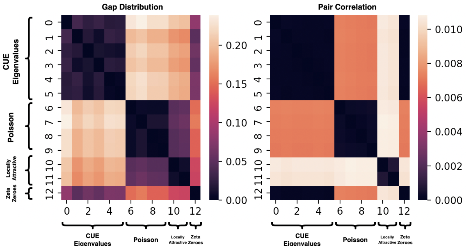
The structural differences of the various types of processes can be quantified through the computation of the Wasserstein distance among all pairs of sequences. On Figure 7, we visualize the Wasserstein distances among the four types of sequences for the statistical indicators: gap distribution and pair correlation function.
Experimental Setup
In the following we briefly describe the different point processes we used to generate our data.
-
•
Poisson process: We sample points in the interval with intensity .
-
•
CUE: We generate an unitary matrix, calculate its eigenvalues, and normalize the sequence of eigenvalues as in (1).
-
•
Riemann Zeros: We normalize blocks of consecutive zeros, so that an interval of length contains approximately zeros.
-
•
Locally attractive points: We generate different Gibbs point processes in the interval with density and custom pair-potential function with
As illustrated in Figure 7 sequences of Riemann zeta zeros and sequences of eigenvalues of unitary matrices are structurally very similar. This observation is formalised in the before mentioned pair correlation conjecture of Montgomery and was numerically investigated in Odlyzko (1992; 1987). On the other hand, the locally attractive points are very different from the CUE and Riemann points which are known to be locally repulsive. The Poisson points are neither locally repulsive nor attractive and are as such at an intermediate distance from both, the repulsive and the attractive instances of point sequences.
5.1 Modeling pair correlation
Experiment 3: CUE Eigenvalues revisited
We evaluate the impact of the mixture model on the modeling of another set of point processes, and more specifically the eigenvalues of Circular Unit Ensemble. We know that this class of point processes have locally non-attractive behavior.

For this evaluation, we used a set of sequences derived from CUE computations. Using a standard train/validation/test split, a) we trained SEMM for epochs, b) we probed the trained model to yield simulated sequences, and c) we measured the average gap distribution and pair correlation of the simulated sequences. On Figure 8 we record the measured statistics in checkpoints: one in the case where the model is not yet trained (the simulated sequences are the result after the 1st training epoch), and one in the case where the case is fully trained on the train set. As we can observe, the trained model is able to simulate properly the CUE sequences, as both gap distribution and pair correlation are matched.
Experiment 4: Poisson Process revisited
Next, we repeat the evaluation setup for the class of Poisson processes. Here, we give two examples of processes, specifically the a) non-stationary, and b) stationary Poisson processes. Following the same experimental protocol with CUE sequences, we probe the trained SEMM model to extend the two types of sequences for a set of next terms.
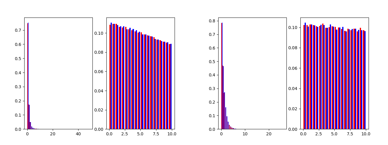
We can observe on Figure 9 that the trained SEMM model is able to model and extend accurately the Poisson processes. Specifically, in the case of the non-stationary processes, SEMM is able to replicate the monotone behavior of the pair correlation function.
Experiment 5: Locally Attractive Processes
Similarly to the CUE and Poisson processes, we next probe the simulation capabilities of SEMM for locally attractive processes. Once again, we utilize actual sequences, and we simulate next terms.
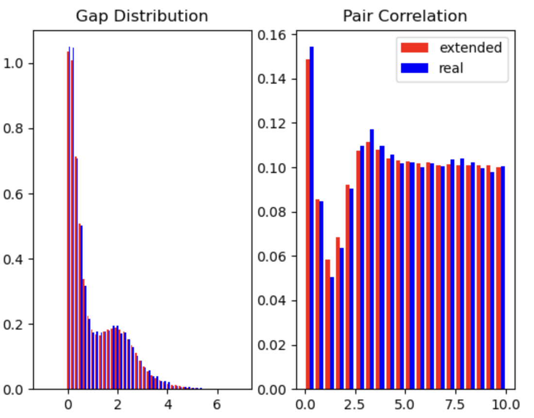
On Figure 10, we observe the simulated gap distribution and pair correlation. We can note that the model yields slightly worse statistical indicators, with respect to CUE and Poisson processes, showcasing the hardness of modeling locally attractive processes.
Ablation Study
In Table 1, we show the ablation study of the Sequence Extension Mixture Model with respect to the size of the context representation, as well as the number of mixture components for the case of gap distribution. The first conclusion from the results is that different configurations are suitable for each sequence category. Specifically, while for the CUE, and the locally attractive sequences, the higher number of mixture components () was more effective, for the case of the Poisson sequences, mixture components suffice. This can be related to the fact that the structural complexity of the gap distribution function seems lower than in the case of CUE, and locally attractive sequences.
Comparison with Neural Networks
In order to show the superiority of the mixture models for modeling sequences, we benchmark a case of neural network architectures that perform multiple next-term prediction (500 multiple steps, following the sampling size of future samples of LMNN). Specifically, we utilize:
-
i)
a fully connected neural network (FCNN) model with 5 layers, that takes as input features the first 500 observed values of the simulated sequences. The output is a multi-label vector (# labels = 500), that describes the extended sequence terms.
-
ii)
a gated recurrent neural network model (GRU), following Equation 6. The basic difference between the GRU architecture, and LMNN model is that the latter learns the parameters of the generating distribution, while the former learns to predict directly the next terms, given the observed values.
In Table 1, we incorporate the results for the two architectures for comparison with the LMNN configurations. We can observe that both models fail to reach the simulation performance of the mixture models. Especially, FCNN exhibits the worst behavior, showcasing the inability of multi-step predictors to learn future terms of long horizon.
| Poisson | CUE | Attractive | ||||
| Model | RMSE () | () | RMSE () | () | RMSE () | () |
| FCNN | 0.282 0.031 | 0.59 0.01 | 0.310 0.14 | 0.53 0.04 | 0.298 0.062 | 0.54 0.03 |
| GRU | 0.238 0.012 | 0.71 0.01 | 0.256 0.050 | 0.66 0.02 | 0.221 0.055 | 0.71 0.02 |
| LMNN - (64-16) | 0.160 0.020 | 0.84 0.02 | 0.185 0.018 | 0.80 0.01 | 0.200 0.021 | 0.77 0.01 |
| LMNN - (64-32) | 0.133 0.015 | 0.86 0.02 | 0.170 0.016 | 0.81 0.02 | 0.212 0.023 | 0.76 0.01 |
| LMNN - (16-64) | 0.170 0.018 | 0.83 0.01 | 0.195 0.017 | 0.78 0.02 | 0.210 0.020 | 0.76 0.02 |
| LMNN - (32-64) | 0.165 | 0.84 0.02 | 0.190 0.015 | 0.79 0.02 | 0.205 0.019 | 0.77 0.02 |
| LMNN - (64-64) | 0.145 0.021 | 0.85 0.01 | 0.194 0.017 | 0.78 0.01 | 0.188 0.018 | 0.79 0.01 |
5.2 Case study: Learning zeroes of the function
One particular case where such model predictions can be useful is the modeling of the real-valued zeroes of the function Vartziotis & Merger (2018). The majority of the ML-based approaches for the extension of the function zeroes Kampe & Vysogorets (2018) are based on the next-term prediction, where given a subsequence of terms, the objective is to predict the term. However, such an objective can become trivial, when the ML models can be overfitted with a large amount of sequence terms for training. Here, we test the performance of LMNN model in a more difficult setup: the multiple-step prediction, where given sequence terms, we predict the next terms with Similarly to Section 5.1, we use a set of cropped, and normalized sequences of the function zeroes for training. Then, given as input a zeroes subsequence with length terms, we probe the model to simulate the next terms.
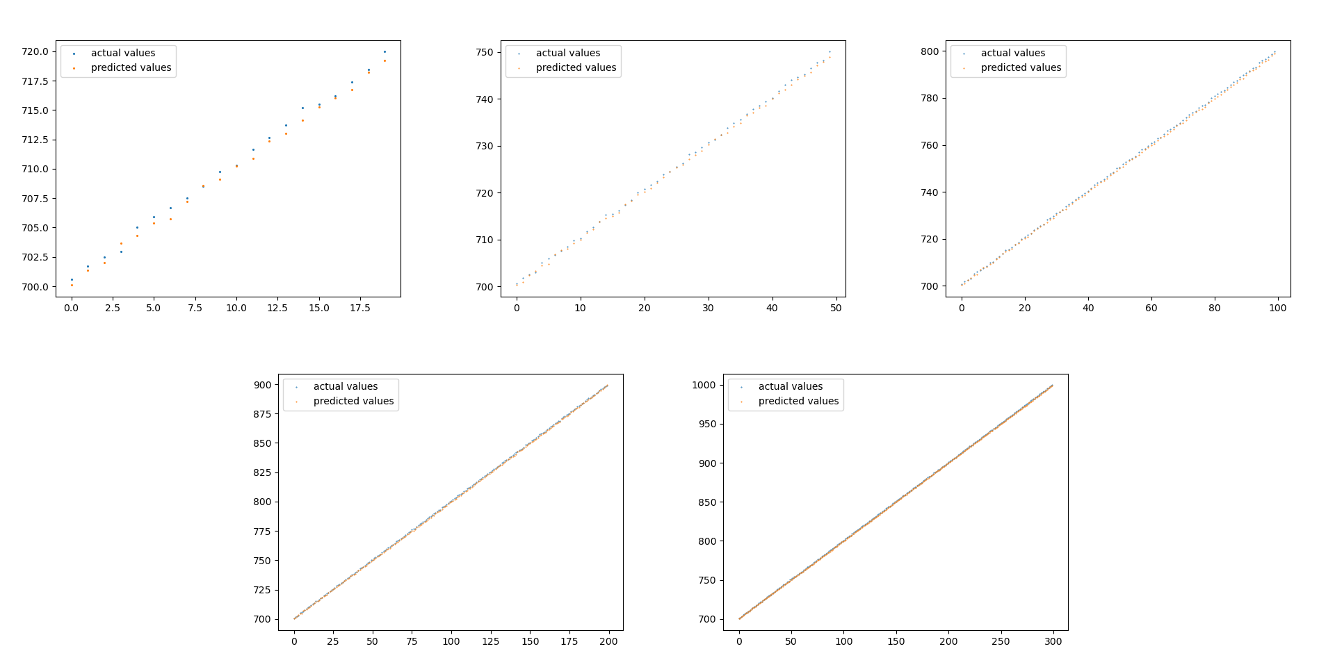
On Figure 11, we present the comparison plots between the actual real-valued zeroes and the predicted ones for an increasing amount of data points . A quite interesting observation is that even for the furthest points of prediction, the estimation error remains close to constant. This highlights a superior advantage of the model, where although the prediction errors should aggregate moving from one term to the next one, the difference in future-step predictions remains independent.
6 Conclusion
In this work, we explore the potential of machine learning for point processes and its contribution to modern mathematics. We build upon a mixture model-based method to extend sequences of real numbers while preserving their statistical properties. Through rigorous experimentation, we evaluated the mixture model’s efficacy on a diverse range of sequences, from Poisson sequences to the eigenvalues of the circular unit ensemble. Our findings underscored the model’s superior performance in both term prediction and retention of gap distribution and pair correlation function, especially when juxtaposed with traditional neural network architectures. A standout case study on the zeroes of the function further solidified our model’s prowess, showcasing its ability to predict values with remarkable accuracy.
7 Acknowledgements
We would like to thank Dr. Michael Keckeisen, TWT, for the valuable discussions.
References
- Ahmad et al. (2020) Iftikhar Ahmad, Muhammad Yousaf, Suhail Yousaf, and Muhammad Ovais Ahmad. Fake news detection using machine learning ensemble methods. Complexity, 2020:1–11, October 2020. doi: 10.1155/2020/8885861. URL https://doi.org/10.1155/2020/8885861.
- Babu & Feigelson (1996) Gutti Jogesh Babu and Eric D. Feigelson. Spatial point processes in astronomy. Journal of Statistical Planning and Inference, 50(3):311–326, March 1996. doi: 10.1016/0378-3758(95)00060-7. URL https://doi.org/10.1016/0378-3758(95)00060-7.
- Beutler & Leneman (1966) Frederick J. Beutler and Oscar A.Z. Leneman. Random sampling of random processes: Stationary point processes. Information and Control, 9(4):325–346, August 1966. doi: 10.1016/s0019-9958(66)80001-3. URL https://doi.org/10.1016/s0019-9958(66)80001-3.
- Celeux et al. (2018) Gilles Celeux, Sylvia Fruewirth-Schnatter, and Christian P. Robert. Model selection for mixture models - perspectives and strategies, 2018.
- Chen et al. (2021) Guohai Chen, Guiqiang Guo, Kaisheng Yang, and Dixiong Yang. Multi-step prediction of zero series and gap series of riemann zeta function. Results in Physics, 27:104449, August 2021. doi: 10.1016/j.rinp.2021.104449. URL https://doi.org/10.1016/j.rinp.2021.104449.
- Cho et al. (2014) Kyunghyun Cho, Bart van Merriënboer, Caglar Gulcehre, Dzmitry Bahdanau, Fethi Bougares, Holger Schwenk, and Yoshua Bengio. Learning phrase representations using rnn encoder-decoder for statistical machine translation. In Proceedings of the 2014 Conference on Empirical Methods in Natural Language Processing (EMNLP), 2014.
- Cox & Isham (2018) D.R. Cox and Valerie Isham. Point Processes. Routledge, December 2018. doi: 10.1201/9780203743034. URL https://doi.org/10.1201/9780203743034.
- Daley & Vere-Jones (2003) D J Daley and David Vere-Jones. An introduction to the theory of point processes. Probability and Its Applications. Springer, New York, NY, 2 edition, November 2003.
- Du et al. (2016) Nan Du, Hanjun Dai, Rakshit Trivedi, Utkarsh Upadhyay, Manuel Gomez-Rodriguez, and Le Song. Recurrent marked temporal point processes: Embedding event history to vector. In Proceedings of the 22nd ACM SIGKDD International Conference on Knowledge Discovery and Data Mining, KDD ’16, pp. 1555–1564, New York, NY, USA, 2016. Association for Computing Machinery. ISBN 9781450342322. doi: 10.1145/2939672.2939875. URL https://doi.org/10.1145/2939672.2939875.
- Dyson (1962) F. J. Dyson. The threefold way. Algebraic structure of symmetry groups and ensembles in quantum mechanics. J. Math. Phys., 3:1199–1215, 1962.
- Fox (1978) Ronald Forrest Fox. Gaussian stochastic processes in physics. Physics Reports, 48(3):179–283, December 1978. ISSN 0370-1573. doi: 10.1016/0370-1573(78)90145-x. URL http://dx.doi.org/10.1016/0370-1573(78)90145-X.
- Gatrell et al. (1996) Anthony C. Gatrell, Trevor C. Bailey, Peter J. Diggle, and Barry S. Rowlingson. Spatial point pattern analysis and its application in geographical epidemiology. Transactions of the Institute of British Geographers, 21(1):256, 1996. ISSN 0020-2754. doi: 10.2307/622936. URL http://dx.doi.org/10.2307/622936.
- Girotti (2022) M. Girotti. Random matrix theory in a nutshell. part i: Determinantal point processes. Lecture Notes. Available online: http://mitliagkas.github.io/ift6085-2020/student-notes-RMT-ML.pdf, 2022.
- Haenggi (2017) Martin Haenggi. User point processes in cellular networks. IEEE Wireless Communications Letters, 6(2):258–261, 2017. doi: 10.1109/LWC.2017.2668417.
- Jang et al. (2017) Eric Jang, Shixiang Gu, and Ben Poole. Categorical reparameterization with Gumbel-softmax. International Conference on Learning Representations, 2017.
- Johnson (1996) Don H. Johnson. Point process models of single-neuron discharges. Journal of Computational Neuroscience, 3(4):275–299, December 1996. ISSN 1573-6873. doi: 10.1007/bf00161089. URL http://dx.doi.org/10.1007/BF00161089.
- Kampe & Vysogorets (2018) J Kampe and A. Vysogorets. Predicting zeros of the riemann zeta function using machine learning: A comparative analysis. preprint available online: https://www.sci.sdsu.edu/math-reu/2018-2.pdf, 2018.
- Katz & Sarnak (1999) Nicholas M. Katz and Peter Sarnak. Zeroes of zeta functions and symmetry. Bull. Am. Math. Soc., New Ser., 36(1):1–26, 1999.
- Kulesza & Taskar (2012) Alex Kulesza and Ben Taskar. Determinantal Point Processes for Machine Learning. Now Publishers Inc., Hanover, MA, USA, 2012. ISBN 1601986289.
- Last & Penrose (2018) G. Last and M. Penrose. Lectures on the Poisson process. Cambridge University Press, Cambridge, 2018.
- Li et al. (2018) Shuang Li, Shuai Xiao, Shixiang Zhu, Nan Du, Yao Xie, and Le Song. Learning temporal point processes via reinforcement learning. In S. Bengio, H. Wallach, H. Larochelle, K. Grauman, N. Cesa-Bianchi, and R. Garnett (eds.), Advances in Neural Information Processing Systems, volume 31. Curran Associates, Inc., 2018. URL https://proceedings.neurips.cc/paper_files/paper/2018/file/5d50d22735a7469266aab23fd8aeb536-Paper.pdf.
- Mariet & Sra (2015) Zelda Mariet and Suvrit Sra. Fixed-point algorithms for learning determinantal point processes. In Proceedings of the 32nd International Conference on International Conference on Machine Learning - Volume 37, ICML’15, pp. 2389–2397. JMLR.org, 2015.
- Mei & Eisner (2017) Hongyuan Mei and Jason Eisner. The neural hawkes process: A neurally self-modulating multivariate point process. In Proceedings of the 31st International Conference on Neural Information Processing Systems, NIPS’17, pp. 6757–6767, Red Hook, NY, USA, 2017. Curran Associates Inc. ISBN 9781510860964.
- Mohler et al. (2011) G. O. Mohler, M. B. Short, P. J. Brantingham, F. P. Schoenberg, and G. E. Tita. Self-exciting point process modeling of crime. Journal of the American Statistical Association, 106(493):100–108, March 2011. doi: 10.1198/jasa.2011.ap09546. URL https://doi.org/10.1198/jasa.2011.ap09546.
- Montgomery (1972) H.L. Montgomery. The pair correlation of zeros of the zeta function. In Analytic number theory (Proceedings of Symposium in Pure Mathemathics, Vol. 24 (St. Louis Univ., St. Louis, Mo., 1972)). American Mathematical Society, 1972.
- Monti et al. (2019) Federico Monti, Fabrizio Frasca, Davide Eynard, Damon Mannion, and Michael M Bronstein. Fake news detection on social media using geometric deep learning. ICLR, 2019. URL https://rlgm.github.io/papers/34.pdf.
- Odlyzko (1987) A.M. Odlyzko. On the distribution of spacings between zeros of the zeta function. Math. Comp. 48: 273-308, 1987.
- Odlyzko (1992) A.M. Odlyzko. The -th zero of the riemann zeta function and 175 millions of its neighbors. Available online: http://www.dtc.umn.edu/ odlyzko/unpublished/zeta.10to20.1992.pdf, 1992.
- Omi et al. (2019) Takahiro Omi, Naonori Ueda, and Kazuyuki Aihara. Fully Neural Network Based Model for General Temporal Point Processes. Curran Associates Inc., Red Hook, NY, USA, 2019.
- Paiva et al. (2019) Felipe Dias Paiva, Rodrigo Tomás Nogueira Cardoso, Gustavo Peixoto Hanaoka, and Wendel Moreira Duarte. Decision-making for financial trading: A fusion approach of machine learning and portfolio selection. Expert Systems with Applications, 115:635–655, January 2019. doi: 10.1016/j.eswa.2018.08.003. URL https://doi.org/10.1016/j.eswa.2018.08.003.
- Perman et al. (1992) Mihael Perman, Jim Pitman, and Marc Yor. Size-biased sampling of poisson point processes and excursions. Probability Theory and Related Fields, 92(1):21–39, March 1992. doi: 10.1007/bf01205234. URL https://doi.org/10.1007/bf01205234.
- Rudnick & Sarnak (1996) Zeév Rudnick and Peter Sarnak. Zeros of principal -functions and random matrix theory. Duke Math. J., 81(2):269–322, 1996.
- Shanker (2019) O. Shanker. Good-to-bad gram point ratio for riemann zeta function. Experimental Mathematics, 30(1):76–85, January 2019. doi: 10.1080/10586458.2018.1492474. URL https://doi.org/10.1080/10586458.2018.1492474.
- Shanker (2022) O. Shanker. Deep learning for riemann zeta function: Large values and karatsuba problem. 2022. doi: 10.13140/RG.2.2.25733.83681. URL https://rgdoi.net/10.13140/RG.2.2.25733.83681.
- Shanker (2012) Oruganti Shanker. Neural network prediction of riemann zeta zeros. Advanced Modeling and Optimization, 14(3):717–728, 2012.
- Shchur et al. (2020) Oleksandr Shchur, Marin Biloš, and Stephan Günnemann. Intensity-free learning of temporal point processes. In International Conference on Learning Representations, 2020. URL https://openreview.net/forum?id=HygOjhEYDH.
- Snyder & Miller (1991) Donald L. Snyder and Michael I. Miller. Random Point Processes in Time and Space. Springer New York, 1991. doi: 10.1007/978-1-4612-3166-0. URL https://doi.org/10.1007/978-1-4612-3166-0.
- Stoyan (2006) Dietrich Stoyan. Fundamentals of Point Process Statistics, pp. 3–22. Springer New York, New York, NY, 2006. ISBN 978-0-387-31144-9. doi: 10.1007/0-387-31144-0˙1. URL https://doi.org/10.1007/0-387-31144-0_1.
- Urschel et al. (2017) John Urschel, Victor-Emmanuel Brunel, Ankur Moitra, and Philippe Rigollet. Learning determinantal point processes with moments and cycles. In Doina Precup and Yee Whye Teh (eds.), Proceedings of the 34th International Conference on Machine Learning, volume 70 of Proceedings of Machine Learning Research, pp. 3511–3520. PMLR, 06–11 Aug 2017. URL https://proceedings.mlr.press/v70/urschel17a.html.
- Vartziotis & Merger (2018) Dimitris Vartziotis and Juri Merger. Contributions to the study of the non-trivial roots of the riemann zeta-function. arXiv preprint arXiv:1804.00913, 2018. URL https://arxiv.org/abs/1804.00913.
- Wasserman (1980) Stanley Wasserman. Analyzing social networks as stochastic processes. Journal of the American Statistical Association, 75(370):280–294, June 1980. ISSN 1537-274X. doi: 10.1080/01621459.1980.10477465. URL http://dx.doi.org/10.1080/01621459.1980.10477465.
- Zuo et al. (2020) Simiao Zuo, Haoming Jiang, Zichong Li, Tuo Zhao, and Hongyuan Zha. Transformer hawkes process. In Proceedings of the 37th International Conference on Machine Learning, ICML’20. JMLR.org, 2020.