Impact of temporal correlations, coherence, and postselection on two-photon interference

Abstract

Two-photon interference is an indispensable resource of quantum photonics, nevertheless, not straightforward to achieve. The cascaded generation of photon pairs intrinsically contain temporal correlations, which negatively affect the ability of such sources to perform two-photon interference, hence hindering applications. We report on how such correlation interplays with decoherence and temporal postselection, and under which conditions the temporal postselection could improve the two-photon interference visibility. Our study identifies crucial parameters of the performance and indicates the path towards achieving a source with optimal performance.

Photons are extremely well suited for the role of flying qubits due to their ease of generation, ability to carry encoding in various degrees of freedom, and low decoherence due to low interaction with the environment. The latter comes at a cost of a limited means to enable photons to interact. The most used method to achieve photon interaction is the two-photon interference on a beamsplitter, also known as the Hong-Ou-Mandel interference Hong1987 . The use of this effect spans numerous platforms and applications, including operations such as teleportation Bouwmeester and entanglement swapping Zukowski , linking quantum systems Beugnon ; Krutyanskiy , photonic circuits Wang2020 , fusing of photonic states Cogan , and state control and characterization Walker . Spontaneous parametric downconversion and quantum dots are the two systems most commonly used to generate bi-partite photon entanglement. In the case of spontaneous parametric downconversion the high two-photon interference contrast is engineered by modification of the joined-spectral amplitude Grice and elimination of the underlying correlations by means of spectral filtering.

In contrast to spontaneous parametric down conversion, where the two photons are generated simultaneously, a quantum dot emits a pair of photons as a time-ordered cascade where the biexciton photon precedes the exciton one. The resulting two-photon wave function describing the cascade emission has the following form Huang1993 ; simon2005

$$\psi(t_{b},t_{x})=2\sqrt{\Gamma_{b}\Gamma_{x}}\mathrm{e}^{-\Gamma_{b}t_{b}}\Theta(t_{b})\mathrm{e}^{-\Gamma_{x}(t_{x}-t_{b})}\Theta(t_{x}-t_{b}),$$ (1)

where $t_{b}$ ($t_{x}$) is the emission time of the biexciton (exciton) photon, while $\Gamma_{b}$ ($\Gamma_{x}$) denotes the biexciton (exciton) decay rate. The factor $\Theta(t_{x}-t_{b})$ has the form of a Heaviside step function and accounts for the time ordering (cascade emission) of the emitted photons. The time ordering induces correlations between the photons of a pair Huang1993 ; simon2005 . The extent of correlations between the two emitted photons, and hence, the purity of a single photon pertaining to a pair, can be quantified by determining the trace of the squared reduced density operator Zyczkowski . Due to the form of the two-photon wave function, $\psi(t_{b},t_{x})$, tracing over the subsystem of the biexciton (exciton) photon will reveal that exciton (biexciton) is not in a pure state. For example, by denoting $\rho_{x}=\Tr_{b}(\psi^{*}\psi)$, we obtain simon2005 the purity of the exciton photon, as

$$\Tr(\rho_{x}^{2})=\frac{\Gamma_{b}}{\Gamma_{b}+\Gamma_{x}}.$$ (2)

The upper bound of $\Tr(\rho_{x}^{2})$ is unity and manifests itself in the case the state is pure. Hence, $\Gamma_{x}\gg\Gamma_{b}$ indicates that the temporal correlations described by $\psi(t_{b},t_{x})$ are strong and that they would lead to a reduction of purity of the individual photons pertaining to a photon pair. On the other hand, $\Gamma_{x}\ll\Gamma_{b}$ implies high purity, a condition required to achieve high visibility contrast in two-photon interference experiments.

The relation between of the decay rates of the biexciton and exciton in a quantum dot embedded in a bulk material is found to be constant, with the biexciton photon decaying approximately twice as fast as the exciton photon. Consequently, the two-photon interference visibility observed in the experiments rarely exceeded 0.5 Rota2020 . On the other hand, the ability to employ photon pairs generated by a single quantum dot in experiments that rely on two-photon interference Bouwmeester ; Zukowski , is an essential requirement for utilization of such sources. Therefore, there is a need for an in depth analysis of the origins of the low interference contrast and mitigation strategies. Here, we theoretically and experimentally investigate how the visibility of the two-photon interference is affected by of temporal correlations, decoherence, and the temporal postselection. Our findings identify the strategy required to maximize the visibility.

The measurements were performed using an In(Ga)As quantum dot embedded in a micropillar cavity. The cavity was designed to feature a low quality factor (200-300) and in return provide a bandwidth of $\sim$5 nm laia2022 . The quantum dot was excited resonantly by means of two-photon resonant excitation of the biexciton jayakumar2013 . To this end, we employed an excitation laser featuring 80 MHz repetition rate and a pulse length of 15 ps. The excess laser scattering was removed by means of spectral and polarization filtering. The biexciton and exciton single photons were separated using a diffraction grating and coupled into single mode fibers. The low multi-photon contribution in the quantum dot emission was confirmed by measuring the auto-correlation function (shown in sup ). The measurements yield $g^{(2)}(0)_{b}$=0.0144(19) for biexciton and $g^{(2)}(0)_{x}$=0.0074(11) for exciton photons. We also performed lifetime measurements and obtained $\tau_{b}=237.16(59)$ ps and $\tau_{x}=367.61(99)$ ps for the biexciton and exciton, respectively (data plots and the respective fits are given in sup ). The ratio of the lifetimes indicates that the correlations between the biexciton and the exciton emission time should significantly reduce the purity of the individual photons Huber13 . However, to determine the upper bound of the two-photon interference visibility we had to employ a theoretical model.

We modeled the quantum dot as a three-level system consisting of a ground state, exciton, and biexciton, as shown in Fig. 1a. Once the quantum dot is two-photon resonantly excited it decays to the ground state via emission of photons with frequencies $\omega_{1}$ (biexciton) and $\omega_{2}$ (exciton). The full description of the system dynamics is given in sup .

Two indistinguishable photons impinging on the beamsplitter will undergo interference hong1987 . If we denote the beamsplitter input modes as a and b, the time-resolved interference of two photons emitted by independent sources is given by Legero ; Kiraz2004

$$G^{(2)}_{HOM}(t,\tau)=\frac{1}{2}\left[\expectationvalue{\xi^{\dagger}_{a}(t)\xi_{a}(t)}\expectationvalue{\xi^{\dagger}_{b}(t+\tau)\xi_{b}(t+\tau)}\right.\\ \left.-2\Re{\left(G^{(1)}_{a}(t,\tau)\right)^{*}G^{(1)}_{b}(t,\tau)}\right].$$ (3)

In the equation above the $n_{a}(t)=\expectationvalue{\xi^{\dagger}_{a}(t)\xi_{a}(t)}$ and $n_{b}(t+\tau)=\expectationvalue{\xi^{\dagger}_{b}(t+\tau)\xi_{b}(t+\tau)}$ are values of photon number in modes a and b and, as such, are proportional to the intensity in the respective mode. On the other hand, $G^{(1)}_{a,b}(t,\tau)$ is the first-order (field) correlation function. The function describing the two-photon interference is the second-order (intensity) correlation function $G^{(2)}_{HOM}(t,\tau)$.

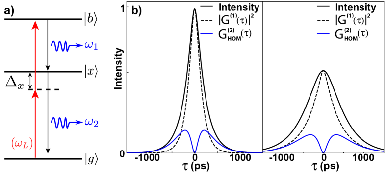
Figure 1: (a) Schematic of the three-level system. A laser with frequency $\omega_{L}$ coherently couples the ground state, $\ket{g}$, and the biexciton, $\ket{b}$, via a virtual level. Upon excitation the biexciton photon, $\omega_{1}$, and exciton photon, $\omega_{2}$, are emitted. The two-photon resonance is detuned from the single photon resonance (ground state, $\ket{g}$, to exciton, $\ket{x}$) by $\Delta_{x}$. (b) The results of the sensor method simulation: intensity, first-order correlation function, $G^{(1)}(\tau)$ and second-order correlation function, $G^{(2)}_{HOM}(\tau)$, for the biexciton (left) and the exciton (right). For optimal comparison of the two plots, the area under the intensity peak was scaled to unity. The simulation assumed the experimentally determined biexciton and exciton lifetimes ($\tau_{b}=237.16(59)$ ps and $\tau_{x}=367.61(99)$ ps) and no dephasing. These results yield two-photon coincidence probability of $P_{0}=0.15$ while the visibility is equal to $\nu$=0.54 for both the biexciton and the exciton photon.

To calculate the first-order correlation function, we implemented the sensor method delvalle2012 . This approach is based on supplementing the three-level system by weakly coupled quantized radiation modes (two-level systems) that act as sensors. Here, we introduced two such sensors (one per emission frequency) and they are described by the following Hamiltonian

$$H_{s}=\sum_{j=1}^{2}\left\{\omega_{j}\xi^{\dagger}_{j}\xi_{j}+g\left[\left(\sigma_{xb}+\sigma_{gx}\right)\xi^{\dagger}_{j}+\mathrm{h.c.}\right]\right\},$$ (4)

where $\omega_{j}$ is the resonance frequency, while $\xi^{\dagger}_{j}$ $(\xi_{j})$ correspond to the creation (annihilation) operator for a sensor $j$. The coupling strength between the sensors and the quantum dot is given by $g$. The presence of the sensors must not perturb the three-level system by, for example, introducing back action from the sensed excitation. Therefore, the parameter $g$ must be very small (we consider $g=10^{-3}$). The detailed description of the sensor method is given in sup .

Sensor method enables the treatment of photon correlations taking into account the uncertainties in time and frequency of the detection delvalle2012 . Hence, it is the ideal approach to quantify the correlations present in quantum dot emission. We employed it to calculate the photon number and the first-order correlation function of the sensor modes. By replacing these in (3) and integrating over $t$, we obtain the $G^{(2)}_{HOM}(\tau)$. Similarly, by integrating the individual terms in (3) one obtains the correlation in photon number and $G^{(1)}(\tau)$, respectively. The results are shown in Fig. 1b. They yield the probability of a coincidence at the outputs of the beamsplitter of $P_{0}=0.15$. While this value is significantly lower than the classical limit of $P_{\infty}=0.5$, imposed by full absence of the interference effect, it demonstrates the detrimental effect of the temporal correlations. The corresponding visibility $\nu$ is 0.54, where the visibility is defined as $(P_{\infty}-P_{0})/(P_{\infty}+P_{0})$ Kaltenbaek2006 .

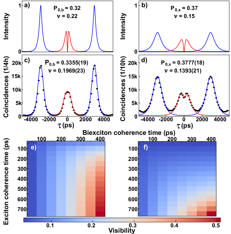
Figure 2: The results of the sensor model calculation for a) biexciton and b) exciton. We assumed the coherence length of biexciton and exciton to be $\tau_{cb}$=200 ps and $\tau_{cx}$=450 ps, respectively. The $G^{(2)}_{HOM}(\tau)$ is plotted as the red central peak, while in blue we plotted the profile of the peak that would be achieved if no interference occurs. The $P_{0}$ and the $\nu$ match the experimentally observed ones. Panels c) and d) show the results of the two-photon interference measurement for biexciton and exciton, respectively. The measurement data are shown as points. The solid line is theory prediction achieved by convolution of the curves shown in the panel a) and b) with the response of the detector. The panels e) and f) show the visibility of the biexciton and exciton photon respectively for various values of the biexciton and exciton photon coherence time. The numerical values are given as tables in sup .

We accessed $P_{0}$ and $\nu$ experimentally. To achieve this we employed two unbalanced interferometers with a nominal delay of 3 ns. The first interferometer served to generate two laser pulses required to excite the quantum dot, while the second interferometer we used to observe two-photon interference of photons emitted in two consecutive excitations. The detailed schematic of the setup is given in Huber15 . The results of these measurements are shown as points in Fig. 2c and Fig. 2d for biexciton and exciton, respectively. The measurements yield $P_{0,b}=0.3355(19)$ and $P_{0,x}=0.3777(18)$ for biexciton and exciton, respectively. The values $P_{0,b}$ and $P_{0,x}$ were determined by summing the area under the central peak and dividing it with the sum of the areas of the adjacent peaks Santori2002 . In the absence of the two-photon interference the three peaks would be identical, resulting in $P_{\infty}=0.5$. The corresponding values of the visibility were found to be $\nu_{b}=0.1969(23)$ and $\nu_{e}=0.1393(21)$, respectively. These values indicate that the cascaded emission is not the unique cause for the reduction of the interference contrast, the coexisting effect being the dephasing of the quantum dot levels. However, the degree of dephasing is not straightforward to access for a cascaded decay. Namely, when the quantum dot is driven in the two-level regime exciting resonantly only the exciton, the information on the dephasing is commonly extracted exactly from the two-photon interference measurement Ding16 ; Unsleber . This approach is motivated by slow dephasing mechanisms that cause the methods such as $G^{(1)}$ measurement employing Michelson interferometer to record higher degree of dephasing than commonly observed in a measurement implemented using photons emitted shortly one after another Thoma . As in the case of a three-level system the two-photon interference is reduced by both the dephasing of any of energy levels involved and the cascade correlations, estimation of dephasing induced photon distinguishability becomes significantly more complicated than in the two-level regime.

However, accessing the coherence length and purity of photons pertaining to a cascade is of extreme relevance for any experiment that relies on two-photon interference. Therefore, we investigated this interplay of the cascade-correlations and decoherence induced reduction of the two-photon interference contrast. To this end, we employed again the sensor method. We introduced the dephasing via the Lindblad terms of the master equation sup . This enabled us the determine $G^{(2)}_{HOM}(\tau)$ for any value of the coherence time attributed to either biexciton or exciton. Several examples of $G^{(2)}_{HOM}(\tau)$ we calculated using this method are plotted in Fig. 3 in sup , while the results that most closely match the experimentally observed values of $P_{0,b}$ and $P_{0,e}$ are shown in Fig. 2a and 2b, respectively. To fit the $G^{(2)}_{HOM}(\tau)$ calculated using sensor method shown in Fig. 2a and 2b to the experimental data, the $G^{(2)}_{HOM}(\tau)$ needs to be convoluted with the response of the detector employed in the measurement, resulting in curves shown in Fig. 2c and Fig. 2d. The data fitting confirmed the values of coherence length of $\tau_{cb}$=200(25) ps and $\tau_{cx}$=450(25) ps for biexciton and exciton, respectively. We used this result to determine the dephasing times of the biexciton and exciton,which are 346(74) ps and 1160(167) ps, respectively. As anticipated, the coherence length of the biexciton and exciton are significantly longer than the $G^{(1)}$ values we measured employing the Michelson interferometer, which yielded 193(9) ps and 130(5) ps for biexciton and exciton, respectively.

In addition, we determined the values of the anticipated two-photon interference visibility for a wide range of different values of coherence length. The visibility results are shown in Fig. 2e and Fig. 2f for biexciton and exciton, respectively. Our results show that the visibility for the biexciton photon is unevenly affected by the coherence loss of the biexciton and the exciton. The numerical values of the visibility are given as tables in sup . Furthermore, to achieve a generalized analysis of the problem, we determined the values of the two-photon interference visibility for the same wide range of values of coherence length and ratio between biexciton and exciton lifetime of 1:2 (200 ps and 400 ps). The plots and the table with numerical values are given in sup .

The most common method to eliminate the undesired correlations between a pair of entangled photons is the postselection. While sources based on spontaneous parametric downconversion rely on a spectral postselection Grice , the system we are addressing here asks for temporal postselection. In such a scenario, to improve the purity of the individual photons the biexciton decay needs to be truncated. We performed both a theoretical and an experimental study of such a scenario.

To theoretically address the effect of the temporal postselection on two-photon interference visibility we employed the quantum trajectory approach Carmichael . This method determines single quantum trajectories from the time evolution of the non-hermitian Hamiltonian,

$$H^{\prime}=H_{I}-\frac{\mathrm{i}\hbar}{2}\sum_{k}C^{\dagger}_{k}C_{k},$$ (5)

where $C_{k}$ corresponds to the $k$-th collapse operator and $H_{I}$ is the time independent Hamiltonian describing our three level system together with the sensors (eq. 16 sup ). Each trajectory consists of a continuous evolution governed by $H^{\prime}$ and a quantum jump that takes place at a random time and enables the spontaneous emission. The continuous evolution is described by the operator $U(t)=e^{-iH^{\prime}t/\hbar}$, where the imaginary term of $H^{\prime}$ decreases the norm of the state vector such that $\norm{\ket{\psi(t_{2}>t_{1})}}<\norm{\ket{\psi(t_{1})}}$. To describe the quantum jumps we discretized the time evolution and for each step we computed the norm of the state vector. We compared values of the norm of the state vector with a randomly generated number $r$ ($0\leq r\leq 1$). We assumed that when the condition $\norm{\ket{\psi(t_{1})}}<r$ was satisfied the collapse and the re-normalization of the wavefunction took place.

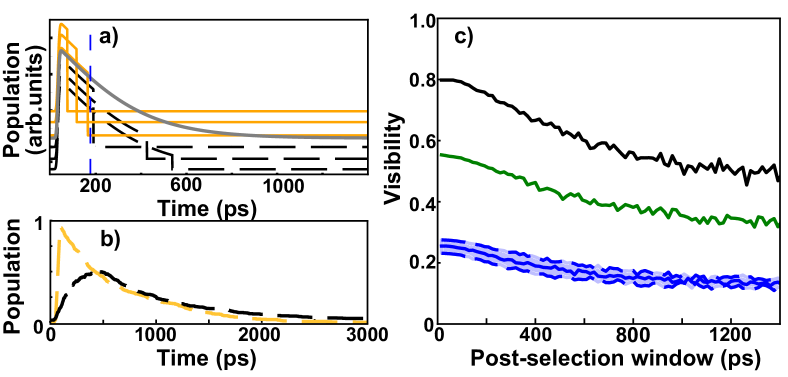
Figure 3: a) The trajectories shown in orange exhibit a quantum jump before the 180 (ps) cut-off (blue dashed line), while the trajectories shown in black feature a quantum jump after the cut-off time. In gray is plotted the change of biexciton population with time calculated as the sum of all possible trajectories. The intensity of the individual plots is given in arbitrary units as the individual curves were vertically displaced for better visual presentation. b) The population change with time for exciton when the corresponding biexiton had a postselection cut-off at at 512 ps (back) and 64 ps (orange). c) Theoretically predicted result of postselection for no-dephasing (black), dephasing such that the coherence time of biexciton and exciton is at 80$\%$ of the Fourier-transform limit (green). The parameters of lifetime were equal to ones of the emitter we used in the experiment. In blue is shown the result for our emitter, accounting for the coherence time determined experimentally. The light blue region accounts for the error with which we have determined the coherence time.

While a single trajectory corresponds to the single evolution of the initial state under a random collapse condition, an averaged set of $N$ trajectories ($N\rightarrow\infty$) approximates the density operator $\rho(t)$ commonly obtained by the solution of the ensemble quantum master equation. Hence, having a numerical solution for a large number of trajectories we can simulate the effect of the temporal postselection based on the biexciton emission happening before a specific time (Fig. 3a). Such a postselection procedure modifies the shape of the corresponding exciton wavepacket (Fig.3b). This, the postselection effectively truncates the biexciton wavepacket, increasing the purity of the exciton reduced density matrix. The increase of the visibility as a consequence of the temporal postselection is shown in the Fig. (Fig.3c).

To experimentally test the effect of the postselection we performed a measurement where we conditioned the detection of the exciton two-photon interference on a detection of a biexciton. In this way, we could employ the time of arrival of the biexciton (time of biexciton detection) as the postselection criterion. The results are shown in Fig. 4. The experimentally observed effect of the postselection is stronger than theoretically predicted, specifically for the short postselection windows. However, one has to note that the measurement statistics for such a short postselection is limiting the accuracy of the measurement.

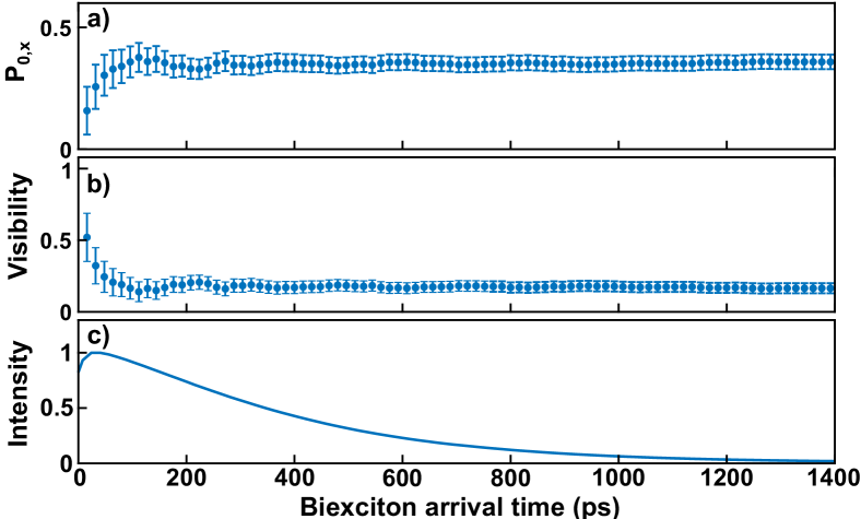
Figure 4: a) The probability of a coincidence at the output of the beamsplitter for exciton photon $P_{0,x}$ and b) the visibility, respectively. Both of these results were achieved in a measurement conditioned by biexciton detection and plotted as a function of the size of the postselection window. c) Lifetime of the biexciton used to define the postselection window.

The concept of the correlation of the photons emitted in a cascading process can be generalized to the phenomenon of time-energy entanglement introduced by Franson Franson1989 . The manifestation of Franson’s interference relies on two properties of the emission time: the uncertainty when a cascade will be emitted and the strong correlations of the photons pertaining to a cascade. This property of the quantum dot emission was recently exploited to demonstrate time-energy entanglement Hohn2023 . However, any other application of entangled photon pairs generated by a quantum dot asks for full elimination of the cascade-induced correlations.

We analysed the combined effect of the decoherence and the cascade-induced correlations on the visibility of the two-photon interference of biexiciton (exciton) photons consecutively emitted by a semiconductor quantum dot. We showed that using the sensor method and the two-photon interference measurement one can access the coherence times of the biexciton and the exciton photon. We generalized our findings and shown that, with respect to two-photon interference visibility the biexicton and exciton photons do not respond evenly to the loss of coherence. Furthermore, we adressed the temporal postselection as a method to improve the visibility of the two-photon interference. Our findings indicate that an improvement is possible, however, only in the absence of dephasing mechanisms that commonly set the quantum dot emission far from being Fourier-transform limited. This finding has an important consequence, it indicates the adequate approach to design photonic cavities that can improve the performance of the quantum-dot-based sources of entangled photon pairs. Namely, not only the emission rate of the biexciton needs to be modified such to eliminate the cascade induced correlations, but the exciton emission rate needs to modified to overcome the dephasing.

- (1) C. K. Hong, Z. Y. Ou, and L. Mandel Phys. Rev. Lett. 59, 2044 (1987).
- (2) D. Bouwmeester, J.-W. Pan, K. Mattle, M. Eibl, H. Weinfurter, and Anton Zeilinger, Nature 390, 575 (1997).
- (3) D. Fattal, E. Diamanti, K. Inoue, and Y. Yamamoto, Phys. Rev. Lett. 92, 037904 (2004).
- (4) M. Żukowski, A. Zeilinger, M. A. Horne, and A. K. Ekert, Phys. Rev. Lett. 71, 4287 (1993).
- (5) J. Beugnon, M. P. A. Jones, J. Dingjan, B. Darquié, G. Messin, A. Browaeys, and P. Grangier, 440, 779 (2006).
- (6) V. Krutyanskiy, M. Galli, V. Krcmarsky, S. Baier, D. A. Fioretto, Y. Pu, A. Mazloom, P. Sekatski, M. Canteri, M. Teller, J. Schupp, J. Bate, M. Meraner, N. Sangouard, B. P. Lanyon, and T. E. Northup, Phys. Rev. Lett. 130, 050803 (2023).
- (7) J. Wang, F. Sciarrino, A. Laing, and M. G. Thompson, Nature Photonics 14, 273 (2020).
- (8) D. Cogan, Z.-E. Su, O. Kenneth, and D. Gershoni, Nature Photonics 17, 324 (2023).
- (9) T. Walker, S. Vartabi Kashanian, T. Ward, and M. Keller, Phys. Rev. A 102, 032616 (2020).
- (10) W. P. Grice and I. A. Walmsley Phys. Rev. A 56, 1627 (1997).
- (11) H. Huang and J. H. Eberly, J. Mod. Opt. 40, 915 (1993).
- (12) C. Simon and J.-P. Poizat, Phys. Rev. Lett. 94, 030502 (2005).
- (13) K. Zyczkowski, P. Horodecki, A. Sanpera, and M. Lewenstein, Phys. Rev. A 58, 883 (1998).
- (14) M. B. Rota, F. Basso Basset, D. J. Tedeschi, and Rinaldo Trotta, IEEE Journal of Selected Topics in Quantum Electronics 26, 1 (2020).
- (15) L. Ginès, et al. Phys. Rev. Lett. 129, 033601 (2022).
- (16) H. Jayakumar, et al. Phys. Rev. Lett. 110, 135505 (2013).
- (17) Supplemental material
- (18) T. Huber, A. Predojević, H. Zoubi, H. Jayakumar, G. S. Solomon, and G. Weihs, Optics Express 21, 9890 (2013).
- (19) C. K. Hong, Z. Y. Ou, and L. Mandel. Phys. Rev. Lett. 59, 2044 (1987).
- (20) T. Legero, T. Wilk, M. Hennrich, G. Rempe, and A. Kuhn Phys. Rev. Lett. 93, 070503 (2004).
- (21) A. Kiraz, M. Atatüre, and A. Imamoğlu, Phys. Rev. A 69, 032305 (2004).
- (22) E. del Valle, A. Gonzalez-Tudela, F. P. Laussy, C Tejedor, M. J. Hartmann, Phys. Rev. Lett. 109, 183601 (2012).
- (23) R. Kaltenbaek, B. Blauensteiner, M. Żukowski, M. Aspelmeyer, and A. Zeilinger, Phys. Rev. Lett. 96, 240502 (2006).
- (24) T. Huber, A. Predojević, D. Föger, G. Solomon, G. Weihs, New Journal of Physics, 17, 123025 (2015).
- (25) C. Santori, D. Fattal, J. Vucković, G. S. Solomon and Y. Yamamoto, Nature 419, 594 (2002).
- (26) X. Ding, Y. He, Z.-C. Duan, N. Gregersen, M.-C. Chen, S. Unsleber, S. Maier, C. Schneider, M. Kamp, S. Höfling, C.-Y.Lu, and J.-W. Pan, Phys. Rev. Lett. 116, 020401 (2016).
- (27) S. Unsleber, Y.-M. He, S. Gerhardt, S. Maier, C.-Y. Lu, J.-W. Pan, N. Gregersen, M. Kamp, C. Schneider, and S. Höfling, Optics Express 24, 8539 (2016).
- (28) A. Thoma, P Schnauber, M Gschrey, M Seifried, J Wolters, J-H Schulze, A Strittmatter, S Rodt, A Carmele, A Knorr, T Heindel, S Reitzenstein, Phys. Rev. Lett. 116, 033601 (2016).
- (29) H. Carmichael Statistical Methods in Quantum Optics 1: master equations and Fokker-Planck equations, Springer Science and Business Media (1999).
- (30) J. D. Franson Phys. Rev. Lett. 62, 2205 (1989).
- (31) M. Hohn, K. Barkemeyer, M. von Helversen, L. Bremer, M. Gschrey, J.-H. Schulze, A. Strittmatter, A. Carmele, S. Rodt, S. Bounouar, and S. Reitzenstein, Phys. Rev. Research 5, L022060 (2023).