Chiral gauge theory at the boundary between topological phases

Abstract

I show how chiral fermions with an exact gauge symmetry in any representation can appear on the $d$-dimensional boundary of a finite volume $d+1$ dimensional manifold, without any light mirror partners. The condition for it to look like a local $d$-dimensional theory is that gauge anomalies cancel, and that the volume be large. This provides a new paradigm for the lattice regularization of chiral gauge theories.

If understanding a theory means that one can reliably compute consequences of it, then we do not understand the Standard Model – despite tremendous agreement between experimental data and calculations to low orders in perturbation theory in the weak interactions. That is because of the tension in quantum field theory between chiral symmetry and the need to tame UV divergences. Regulating a quantum field theory requires introduction of a UV mass scale, which is difficult to do without breaking chiral symmetry. This tension has physical consequences in the form of anomalies, but it also places an obstacle to defining chiral gauge theories, where violating chiral symmetry means breaking gauge invariance. The Standard Model is an example of a chiral gauge theory, where left and right chirality fermions gave different gauge interactions. While a perturbative lattice regulator has been shown to work to all orders for chiral gauge theories in Ref. [1], neither a perturbative scheme that is known to work to all orders in the continuum nor a nonperturbative lattice formulation for generic chiral gauge theories presently exists.

The tension between chiral symmetry and regularization applies equally to continuum and lattice approaches [2, 3]. Domain wall fermions were introduced to solve the problem of realizing chiral symmetry on the lattice by exploiting the fact that in infinite volume, massless fermion modes must exist on the spatial boundary between two topologically distinct phases [4, 5, 6]. Such phases can be realized by Wilson fermions, depending on the ratio of the fermion mass to the Wilson coupling (the coefficient of $\bar{\psi}\partial^{2}\psi$) [6]. A natural consequence of this lattice construction is being able to correctly account for the anomalous divergence of chiral currents and explicitly observe them [7]. For actual computations on a finite lattice, the topological phase boundaries can be approximately realized as the two edges of a finite 5-dimensional lattice [8]. Our 4d world then consists of the two boundaries of a 5d slab with chiral modes of opposite chirality bound to the two surfaces, with 4d gauge fields independent of the extra dimension. This gives a light Dirac fermion with a chiral symmetry violating mass that vanishes exponentially fast with the extent of the extra dimension. In the limit of infinite extra dimensions, chiral symmetry is restored (up to anomalies), and the massless chiral modes can be described by the overlap operator on a finite 4-dimensional lattice, without reference to the gapped modes in the bulk [9, 10, 11, 12, 13]. In turn, the overlap operator solves the Ginsparg-Wilson equation [14] which implies the existence of exact chiral “Lüscher” symmetries of the lattice action that gives rise to the appropriate anomalous transformation of the lattice integration measure [15].

The domain wall and overlap constructions have led to a complete solution to the problem of constructing vector-like gauge theories with global chiral symmetries, but do not directly lead to a regulator for lattice chiral gauge theory. This is because for every Weyl fermion on one boundary, there is a mirror fermion with opposite chirality on the other boundary, so the overall theory is vector-like. There have been numerous attempts to find a lattice regularization of a chiral gauge theory, using domain wall or overlap fermions as a starting point, or by other approaches .

In this Letter I present an alternative, that our 4d world is the boundary of a finite 5d manifold that has only a single boundary, where that boundary supports chiral edge modes in an arbitrary representation of the gauge group. With the manifold having only a single boundary, there are no mirror fermions. My conclusion is that it is precisely the gauge anomaly cancellation condition that allows this system to behave as a local $d$-dimensional quantum field theory in the IR, and that there is no obvious obstruction to simulating such a system nonperturbatively on a lattice – although there remain unanswered questions. (For earlier related work by Aoki and Fukaya, see Ref. [31]).

Consider a free massive Dirac fermion on the manifold $Y=M^{d-1}\times{\mathbb{R}}^{2}$ with Euclidian signature. The $M^{d-1}$ manifold is described by the $d-1$ coordinates ${\mathbf{x}}_{\perp}$, while the ${\mathbb{R}}^{2}$ submanifold is described by Cartesian coordinates $\{x,y\}$ or polar coordinates $\{r,\theta\}$. The fermion mass, as pictured in Fig. 1, is taken to equal $m$ for $r<R$ and $-M$ for $r>R$, with both $m$ and $M$ real and positive. I will eventually take $M\to\infty$ which will allow ignoring the region $r>R$, in which case $Y=M^{d-1}\times\kern 0.6pt\overline{\kern-0.6ptD\kern-0.6pt}\kern 0.6pt_{R}$, where $\kern 0.6pt\overline{\kern-0.6ptD\kern-0.6pt}\kern 0.6pt_{R}$ is the closed disc of radius $R$, and the boundary of $Y$ is $M^{d-1}\times S^{1}$, which will serve as our spacetime. I take $d$ to be even and the fermions to be Dirac, but the analysis can be generalized to include Majorana fermions and edge states in odd spacetime dimensions, such as recently discussed in Ref. [32].

The fermion action may be written as

$$S=\int d{\mathbf{x}}_{\perp}\int r\,dr\,d\theta\,\kern 0.6pt\overline{\kern-0.6pt\psi\kern-0.6pt}\kern 0.6pt\left(\not{\partial}_{\perp}+{\cal D}\right)\psi\ ,$$ (1)

where $\not{\partial}_{\perp}=\vec{\gamma}_{\perp}\vec{\partial}_{\perp}$ is the Dirac operator on $M^{d-1}$ and

$${\cal D} = \gamma_{x}\partial_{x}+\gamma_{y}\partial_{y}+m(r)$$ (2)

$$= \gamma_{r}\left(\partial_{r}+\frac{1}{2r}\right)+\frac{i}{r}\gamma_{\theta}{\cal J}+m(r),$$ (4)

where

$$\gamma_{r}=\cos\theta\,\gamma_{x}+\sin\theta\,\gamma_{y}\ ,\ \gamma_{\theta}=-\sin\theta\,\gamma_{x}+\cos\theta\,\gamma_{y}\ ,$$ (5)

and ${\cal J}$ is the angular momentum operator

$${\cal J}=-i\partial_{\theta}+\tfrac{1}{2}\Sigma\ ,\qquad\Sigma=-\frac{i}{2}\left[\gamma_{x},\gamma_{y}\right]\ .$$ (6)

Since ${\cal D}$ is not Hermitian it is convenient to expand $\psi$ and $\bar{\psi}$ in the functions $f_{n}$ and $b_{n}$ respectively, which satisfy

$${\cal D}f_{n}=\mu_{n}b_{n}\ ,\qquad\kern 0.6pt\overline{\kern-0.6pt{\cal D}\kern-0.6pt}\kern 0.6ptb_{n}=\mu_{n}^{*}f_{n}\ ,$$ (7)

where

$$\kern 0.6pt\overline{\kern-0.6pt{\cal D}\kern-0.6pt}\kern 0.6pt=\frac{1}{r}{\cal D}^{\dagger}r = -\gamma_{r}\left(\partial_{r}+\frac{1}{2r}\right)-\frac{i}{r}\gamma_{\theta}{\cal J}+m(r)$$ (8)

$$= \Sigma{\cal D}\Sigma$$ (9)

is the adjoint of ${\cal D}$ with respect to the integration measure in polar coordinates. As $f,b$ are eigenstates of the self-adjoint operators $\kern 0.6pt\overline{\kern-0.6pt{\cal D}\kern-0.6pt}\kern 0.6pt{\cal D}$ and ${\cal D}\kern 0.6pt\overline{\kern-0.6pt{\cal D}\kern-0.6pt}\kern 0.6pt$ respectively, they each can be taken to be a complete orthonormal basis. The magnitude of $\mu_{n}$ may be found by solving the eigenvalue equation

$$\kern 0.6pt\overline{\kern-0.6pt{\cal D}\kern-0.6pt}\kern 0.6pt{\cal D}f_{n}=|\mu_{n}|^{2}f_{n}\ ,$$ (10)

and the phase of $\mu_{n}$, can be conveniently fixed by choosing

$$b_{n}=\Sigma f_{n}\ .$$ (11)

Only solutions with low lying eigenvalues $|\mu|<m$ correspond to boundary states.

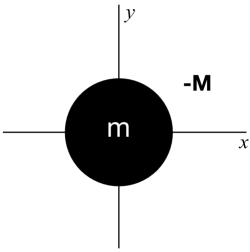
Figure 1: The Dirac fermion mass $m(r)$ in the $x-y$ plane equals $m>0$ within a disc of radius $R$, and $-M<0$ outside, where we will eventually take $M\to\infty$. To simulate the system only the region $r\leq R$ is required, with appropriate boundary conditions.

The cylindrical symmetry of the problem can be exploited by taking $f$ and $b$ to be eigenstates of the angular momentum operator ${\cal J}$ which commutes with both ${\cal D}$ and $\kern 0.6pt\overline{\kern-0.6pt{\cal D}\kern-0.6pt}\kern 0.6pt$ and has eigenvalues $j=\pm\tfrac{1}{2},\pm\frac{3}{2},\ldots$. Therefore a convenient basis to work in is one where the spin $\Sigma$ is diagonal, such as

$$\vec{\gamma}_{\perp}=\sigma_{3}\otimes\vec{\Gamma}\ ,\quad\gamma_{x}=\sigma_{1}\otimes 1\ ,\quad\gamma_{y}=\sigma_{2}\otimes 1\ ,$$ (12)

$$\Sigma=-\frac{i}{2}\left[\gamma_{x},\gamma_{y}\right]=\sigma_{3}\otimes 1\ .$$ (13)

where $\vec{\Gamma}$ are the $2^{d/2-1}\times 2^{d/2-1}$ Dirac matrices in $(d-1)$ dimensions (for example, $\vec{\Gamma}=1$ for $d=2$, and $\vec{\Gamma}=\vec{\sigma}$ for $d=4$). In polar coordinates we have

$$\gamma_{r}=\begin{pmatrix}0&e^{-i\theta}\\ e^{i\theta}&0\end{pmatrix}\ ,\qquad\gamma_{\theta}=\begin{pmatrix}0&-ie^{-i\theta}\\ ie^{i\theta}&0\end{pmatrix}$$ (14)

while $\Sigma$ is unchanged.

The fields $\psi$ and $\bar{\psi}$ can now be expanded as

$$\psi_{\alpha i} = \sum_{n}f_{n,i}(r,\theta)\chi_{n,\alpha}({\mathbf{x}}_{\perp})$$ (15)

$$\bar{\psi}_{\alpha i} = \sum_{n}\bar{\chi}_{n,\alpha}({\mathbf{x}}_{\perp})b^{\dagger}_{n,i}(r,\theta)\ ,$$ (16)

where the spinor index $i=1,2$ is acted on by the first block in our direct product notation for the Dirac matrices, the $\alpha=1,\ldots,2^{d/2-1}$ indices are acted on by the second block, and the $\chi_{n,\alpha}({\mathbf{x}}_{\perp})$ are $2^{d/2-1}$-component spinors. Since ${\cal D}$ only acts on $b$ and $f$, and not on $\chi$, and because ${\cal D}f_{n}=\mu_{n}b_{n}$, it follows that

$$\int d{\mathbf{x}}_{\perp}\int rdrd\theta\,\bar{\psi}{\cal D}\psi=\sum_{n}\int d{\mathbf{x}}_{\perp}\ \mu_{n}\bar{\chi}_{n}\chi_{n}\ ,$$ (17)

Furthermore, since

$$b^{\dagger}_{n}\not{\partial}_{\perp}=f_{n}^{\dagger}\Sigma\not{\partial}_{\perp}=f_{n}^{\dagger}\,(1\otimes\vec{\Gamma})\cdot\vec{\partial}_{\perp}\ ,$$ (18)

we also have

$$\int d{\mathbf{x}}_{\perp}\int rdrd\theta\,\bar{\psi}\not{\partial}_{\perp}\psi=\sum_{n}\int d{\mathbf{x}}_{\perp}\ \bar{\chi}_{n}\vec{\Gamma}\cdot\vec{\partial}_{\perp}\chi_{n}\ .$$ (19)

Putting these two results together, we get that the action can be rewritten as the sum of an infinite tower of fermions propagating on $M^{d-1}$:

$$S=\int d{\mathbf{x}}_{\perp}\,\sum_{n}\bar{\chi}_{n}\left(\vec{\Gamma}\cdot\vec{\partial}_{\perp}+\mu_{n}\right)\chi_{n}\ .$$ (20)

The unnormalized solutions to eq. (7) for the boundary modes on the disc ($r\leq R$) in the $M\to\infty$ limit are given by

$$f_{j}(r) = \begin{pmatrix}e^{i(j-1/2)\theta}\frac{I_{|j-1/2|}(\kappa_{j}r)}{I_{|j-1/2|}(\kappa_{j}R)}\\[8.0pt] -e^{i(j+1/2)\theta}\frac{I_{|j+1/2|}(\kappa_{j}r)}{I_{|j+1/2|}(\kappa_{j}R)}\end{pmatrix}\ ,$$ (21)

$$b_{j}(r) = \begin{pmatrix}e^{i(j-1/2)\theta}\frac{I_{|j-1/2|}(\kappa_{j}r)}{I_{|j-1/2|}(\kappa_{j}R)}\\[8.0pt] e^{i(j+1/2)\theta}\frac{I_{|j+1/2|}(\kappa_{j}r)}{I_{|j+1/2|}(\kappa_{j}R)}\end{pmatrix}\ ,$$ (24)

where $I_{\nu}(z)$ is a modified Bessel function and

$$\kappa_{j}=\sqrt{m^{2}-|\mu_{j}|^{2}}$$ (25)

subject to the implicit eigenvalue condition

$$\mu_{j}=m-\kappa_{j}\frac{I_{|j-1/2|}(\kappa_{j}R)}{I_{|j+1/2|}(\kappa_{j}R)}\ .$$ (26)

In the limit $M\to\infty$ one finds that the $f$ and $b$ solutions obey chiral boundary conditions at the edge of the disc,

$$\frac{1+\gamma_{r}}{2}f_{j}(R)=\frac{1-\gamma_{r}}{2}b_{j}(R)=0\ ,$$ (27)

with $\gamma_{r}$ playing the role of $\gamma_{5}$. in addition to the surface mode solutions there are less interesting bulk excitations labeled by a radial excitation quantum number as well as $j$.

The eigenvalue equation eq. (26) can be solved explicitly in an expansion in inverse powers of $mR$, with the result

$$\mu_{j} = -\frac{j}{R}\left[1+\frac{1}{2mR}+\frac{1}{2m^{2}R^{2}}+\frac{3}{4m^{3}R^{3}}+\frac{3}{2m^{4}R^{4}}\right.$$ (30)

$$\qquad\quad\left.+\frac{15}{4m^{5}R^{5}}\right]$$

$$+\frac{j^{3}}{R}\left[\frac{1}{4m^{4}R^{4}}+\frac{3}{2m^{5}R^{5}}\right]+O\left((mR)^{-6}\right),$$

which is valid for either sign of $j$.

To interpret the boundary mode action we found in eq. (20) with the above expression for $\mu_{j}$ it is useful to consider the Dirac operator in $d$-dimensions in a chiral basis for the $\gamma$-matrices:

$$\vec{\gamma}_{\perp} = \sigma_{1}\otimes\vec{\Gamma}\ ,$$ (31)

$$\gamma_{\parallel} = \sigma_{2}\otimes 1\ ,$$ (32)

$$\gamma_{\chi} = \sigma_{3}\otimes 1\ ,$$ (33)

so that the Dirac operator takes the form

$$\not{\partial}=\begin{pmatrix}0&\vec{\Gamma}\cdot\vec{\partial}_{\perp}-i\partial_{\parallel}\\ \vec{\Gamma}\cdot\vec{\partial}_{\perp}+i\partial_{\parallel}&0\end{pmatrix}$$ (34)

where $\vec{\partial}_{\perp}$ is the gradient in the $(d-1)$ dimensions and $\partial_{\parallel}=\partial/\partial x_{d}$. By Fourier transforming with respect to $x_{d}$ this becomes

$$\not{\partial}=\begin{pmatrix}0&\vec{\Gamma}\cdot\vec{\partial}_{\perp}+p_{\parallel}\\ \vec{\Gamma}\cdot\vec{\partial}_{\perp}-p_{\parallel}&0\end{pmatrix}\ .$$ (35)

Finally, compactifying the $d^{th}$ dimension to a circle of radius $R$ renders $p_{\parallel}$ discrete, $p_{\parallel}\to j/R$, where $j$ takes integer values for periodic boundary conditions, and half integer values for anti-periodic. The two different blocks in $\not{\partial}$ correspond to the fermion operators for the two Weyl fermions of opposite chirality that make up the Dirac fermion, with $\vec{\Gamma}\cdot\vec{\partial}_{\perp}-\frac{j}{R}$ corresponding to a left-handed fermion. This looks very much like the fermion operator for the edge states in the action eq. (20), given the eigenvalues in eq. (30). The corrections in powers of $1/(mR)$ are due to the finite, $j$-dependent extent of the boundary state wave functions into the bulk a distance $O(1/m)$. To order $1/(mR)^{3}$ they are just renormalizing the value of $R$ that appears in the $j/R$ expression. At $O((mR)^{-4})$ a $j^{3}$ contribution appears, corresponding to an irrelevant 3-derivative contribution to the kinetic term of the Weyl fermion, which does not violate chirality. What is interesting is that even though I solved for eigenfunctions that are single-valued in $\theta$, the result is a chiral fermion at the boundary with a spectrum reflecting anti-periodic boundary conditions.

While the $j^{3}$ term corresponds to an irrelevant operator, its appearance suggests that the dispersion relation could become nonanalytic in $j$ for $j\gtrsim mR$. Indeed, that appears to be the case: a graphical solution of eq. (26) shows two eigenvalues merging and going into the complex plane for $j$ roughly equal to $mR$.

The result that an exactly chiral mode exists on the $d$ dimensional boundary of a finite $d+1$ dimensional manifold may seem counter-intuitive. If one were to elongate the disc, the system would look similar to the traditional wall/anti-wall system which supports a right-handed edge state on one side, a left-handed one on the other, and an exponentially small but nonzero mass term from the overlap of their wave functions. The reason why we do not find both chiralities for the disc is because while $\gamma_{5}$ is a constant matrix for the wall/anti-wall system, its analog for the disc, $\gamma_{r}$, is not – and in fact it changes sign from one side of the disc to the other, explaining how modes on opposite sides can have the same chirality. The exponentially small interaction between the two modes on opposite sides of the finite disc can be seen by evaluating the eigenvalue equation eq. (26) at $j=0$ and finding $\mu\sim\exp{-2mR}$; in this case, however, such an interaction does not flip chirality, but instead represents a nonlocality from the $d$-dimensional perspective which vanishes in the large $mR$ limit. This is consistent with the above observation that the dispersion relation for the edge states appears to have a nonanalyticity large $j\sim mR$. It is unclear whether this is a serious flaw with this proposal, or whether the fact that it is exponentially small in $R$ means that the nonlocality is under control.

I now turn to the question of gauging the theory. The $d+1$ dimensional theory with $N$ copies of fermions can be gauged in a straightforward way because the action consists of Dirac fermions with an exact $U(N)$ global symmetry. However, if one wants to describe a $d$-dimensional chiral gauge theory on the boundary, and not a theory of $d$-dimensional surface modes interacting with $d+1$ dimensional gauge fields, one must find a way for the gauge fields in the bulk to be completely determined by their values on the surface, and not have independent bulk degrees of freedom. Therefore we must define a gauge field $B_{\mu}$ over the whole disc in such a way that it only depends on the gauge field’s boundary value,

$$B_{\mu}({\mathbf{x}}_{\perp},r,\theta)\biggl{|}_{r=R}=A_{\mu}({\mathbf{x}}_{\perp},\theta)\ ,$$ (36)

where the $d$-dimensional gauge field $A_{\mu}$ living on the boundary is the field being integrated over in the path integral, subject to the usual measure $e^{-S_{YM}}$, where $S_{YM}$ is the $d$-dimensional Yang-Mills action.

It then becomes possible to understand better the role of gauge anomalies in defining a $d$-dimensional chiral gauge theory using anomaly in-flow arguments. When integrating out the regulated bulk modes, a Chern-Simons operator involving $B_{\mu}$ will be generated in the bulk, and it is the only relevant operator one can expect. With the $B_{\mu}$ fields being nonlocal functionals of the $A_{\mu}$ gauge fields at the boundary, the existence of the Chern-Simons operator will in general preclude interpreting the theory of the edge states as being a local $d$-dimensional gauge theory. However, the exception is when the coefficient of the Chern-Simons operator vanishes, which occurs precisely when the surface modes are in an anomaly-free representation of the gauge theory [33]. Therefore the conclusion is that when the $B_{\mu}$ fields are introduced and their boundary values $A_{\mu}$ are integrated over, the theory will have a local $d$-dimensional description only when the gauge anomalies cancel.

Anomaly inflow and the existence of chiral edge states at the boundary between topological phases are intimately related. Neither makes any sense, however, until the theory is regulated – there is no intrinsic topological meaning to a Dirac fermion with mass $m$ as opposed to $-M$; only when the momentum space for bulk modes is compact do the topological features of the theory emerge. For the continuum theory, the regulator could consist of a Pauli-Villars field with spatially constant mass $-M$, so that the exterior of the disc is topologically trivial (the contributions of the regulator and the fermion to a Chern-Simons operator cancel in the exterior, but add in the interior of the disc). As shown in Ref. [34], the introduction of the regulator solves another unsatisfactory feature of the model described above. The fermion determinant for a chiral fermion in the presence of gauge fields must take the form $\sqrt{\det\not{D}}\exp(i\phi[B])$, where $\det\not{D}$ is the determinant of the massless Dirac operator, and $\phi[B]$ is some functional of $B_{\mu}$ that needs to be uniquely defined in a sensible way. However, the eigenvalues $\mu_{j}$ computed in eq. (30) intrinsically depended on my choice of phase for the $f$ eigenfunctions relative to the $b$ eigenfunctions, as evident in their definition in eq. (7). This phase ambiguity has no consequence in the free theory, but must be eliminated in defining a chiral gauge theory. As in Ref. [34], the phase ambiguity is resolved by a matching ambiguity in contributions from the regulator, and the authors identify the phase $\phi[A]$ with $-\pi\eta[B]$, where $\eta$ is the $\eta$-invariant is the gauge invariant, regulated sum of signs of the eigenvalues of the bulk Dirac operator subject to generalized APS boundary conditions in the presence of the $B_{\mu}$ bulk gauge field The functional $\eta[B]$ is perturbatively related to the Chern-Simons operator, but contains additional information. When the edge states are in a representation free of gauge anomalies, not only does the Chern-Simons contribution cancel, but the phase $\exp(-i\pi\eta[B])$ of the fermion determinant becomes independent of the gauge field in the bulk and only depends on its boundary value, the physical gauge field $A_{\mu}$.

For practical applications one needs a concrete proposal for how to continue the gauge fields into the bulk. One possible definition, considered previously in Refs. [36, 37] for related reasons, is to have $B_{\mu}$ be the solution to the Euclidian equations of motion subject to the above boundary condition,

$$\partial_{r}B_{\mu}=D_{\nu}G_{\mu\nu}\ ,\qquad\mu,\nu=1,\ldots(d-1),\theta\ ,$$ (37)

$$B_{\mu}({\mathbf{x}}_{\perp},R,\theta)=A_{\mu}({\mathbf{x}}_{\perp},\theta)\ ,$$

where

$$D_{\mu} = \partial_{\mu}+[B_{\mu},\cdot]\ ,$$ (38)

$$G_{\mu\nu} = \partial_{\mu}B\nu-\partial_{\nu}B_{\nu}+[B_{\mu},B_{\nu}]\ .$$ (39)

This is referred to as gradient flow, and has been widely used for unrelated applications [38, 39]. One of its features is that it preserves $d$-dimensional gauge invariance, although with the cylindrical geometry, such gauge transformations will be singular at $r=0$. Whether this is a satisfactory solution is not completely clear, and a careful treatment of potential obstacles to continuing the gauge field into the bulk is beyond the scope of this Letter, but needs to be considered more fully. In any case, if the boundary gauge fields $A_{\mu}$ are smooth compared to $m^{-1}$, then the bulk fields $B_{\mu}$ will not change appreciably with respect to $r$ in the vicinity of the boundary, fulfilling the assumption of Ref. [34], in which case the fermion determinant in an anomaly-free chiral gauge theories is expected to be independent of the gauge fields in the bulk.

Finally, we must consider whether the theory can be realized on the lattice. Since the continuum chiral edge states arises at the boundary between two topological phases, and similar topological phases are known to exist for Wilson fermions on the lattice [5, 6], there is no obvious obstacle for realizing the disc construction on the lattice. One would apply the same open boundary conditions discussed in [8]. However, a single Weyl mode in the spectrum would seem to violate the Nielsen-Ninomiya theorem and one of the assumptions going into that theorem must be violated, and it isn’t the existence of chiral symmetry, since we have gauged an exact vectorlike symmetry of the $(d+1)$-dimensional theory. However, note that we obtained a chiral mode in the continuum by assuming that the manifold only had one boundary. If we had considered an annulus instead of a disc, we would not have discarded the $K_{\nu}$ Bessel function modes in the interior of the disc, since they would not be singular at the radius $R^{\prime}$ of the inner edge, and we would have found a mode with opposite chirality on the inner boundary with eigenvalues $+j/R^{\prime}$ instead of $-j/R$, circulating in the opposite sense and corresponding to an edge mode of the opposite chirality, from the $d$-dimension perspective. A lattice, of course, is full of holes. Therefore we can expect to see modes of the opposite chirality at the center of the latticized disc with a dispersion relation resembling $+j/a$. What is interesting about the continuum case with inner mode spectrum $+j/a$ is that it remains discrete in quanta of $1/a$ even as we take the $mR\to\infty$ limit and the dispersion relation of the outer fermion approaches the continuous large-volume dispersion relation. In particular, there will be a gap in the spectrum inner fermion eigenvalues of $O(1/a)$, and no low momentum mode. Thus I speculate that the assumption by Nielsen and Ninomiya that on the infinite volume lattice the fermion dispersion relation can be taken to be continuous and analytic will not hold for this model: it will hold for the Weyl fermion on the outer boundary, but not for the spectrum of the “inner boundary”. Therefore the argument that a continuous periodic function cannot cross zero an odd number of times does not pertain; in this model it will cross the axis smoothly in one direction, but on the return the spectrum jumps discontinuously from one side of the axis to the other. The price, therefore, is some loss of locality in position space. Since these states of opposite chirality will be confined to regions the size of a plaquette, physically separated from the continuum Weyl fermion and ostensibly with no communication between the desired modes and the undesired ones when gauge anomalies cancel, it is not obvious that the continuum limit is threatened by the existence of such states. The mismatch between having a regular lattice and a circular boundary unfortunately precludes the same sort simple analytical solutions for lattice edge states as were found for a domain wall in Refs. [4, 5]. A square lattice is more amenable, but will likely result in an edge state without the full Lorentz symmetry in the continuum. For the free theory, this picture of the spectrum has been corroborated numerically on a square lattice [40].

It is unclear whether a direct simulation of the physical setup described here is the preferred course, or whether a direct computation of the $\eta$-invariant on the solid torus is, perhaps using the techniques described in Ref. [41]. Generically one can expect a sign problem that persists in the continuum limit when simulating a chiral gauge theory, but it is unclear how severe it will be. Perhaps one of the first applications of the idea should be the simulation of a Dirac edge state, where a sign problem does not exist in the continuum. This would allow numerical exploration of potential nonlocality problems, as well as the expected dependence on solely the boundary values of the gauge fields.

This model gives reason for optimism that one can finally achieve a meaningful nonperturbative definition of chiral gauge theories such as the Standard Model. It can also be generalized to consider edge states in odd spacetime dimensions, as well as Majorana edge states. It is hoped that this formulation will allow chiral gauge theories to be simulated on a quantum computer some day, in order to overcome the sign problems and explore the rich phenomenology expected from them.

For traditional domain wall fermions there were convincing effective field theory arguments for why global chiral symmetry became restored in the limit of infinite domain wall separation, but a precise understanding of chirality in this system was not possible until the overlap description of the edge states was discovered and it was shown to obey the Ginsparg-Wilson equation [9]. What is needed for the disc model presented here is some sort of equivalent progress that can shed more light on how chiral symmetry is realized and whether nonlocality issues can be tamed.

I Acknowledgements

I thank M. Golterman, M. Savage, S. Sen, Y. Shamir, and especially J. Kaidi and K. Yonekura for useful conversations and correspondence. This research is supported in part by DOE Grant No. DE-FG02-00ER41132.

References

- Lüscher [2001] M. Lüscher, Chiral gauge theories revisited, Theory and Experiment Heading for New Physics; World Scientific: Singapore , 41 (2001), arXiv:hep-th/0102028 .
- Karsten and Smit [1981] L. H. Karsten and J. Smit, Lattice fermions: species doubling, chiral invariance and the triangle anomaly, Nucl. Phys. B 183, 103 (1981).
- Nielsen and Ninomiya [1981] H. B. Nielsen and M. Ninomiya, Absence of Neutrinos on a Lattice. 1. Proof by Homotopy Theory, Nucl. Phys. B 185, 20 (1981), [Erratum: Nucl.Phys.B 195, 541 (1982)].
- Kaplan [1992] D. B. Kaplan, A method for simulating chiral fermions on the lattice, Phys. Lett. B 288, 342 (1992), arXiv:hep-lat/9206013 .
- Jansen and Schmaltz [1992] K. Jansen and M. Schmaltz, Critical momenta of lattice chiral fermions, Phys. Lett. B 296, 374 (1992), arXiv:hep-lat/9209002 .
- Golterman et al. [1993] M. F. L. Golterman, K. Jansen, and D. B. Kaplan, Chern-simons currents and chiral fermions on the lattice, Phys. Lett. B 301, 219 (1993), arXiv:hep-lat/9209003 .
- Jansen [1992] K. Jansen, Chiral fermions and anomalies on a finite lattice, Physics Letters B 288, 348 (1992), arXiv:hep-lat/9206014 .
- Shamir [1993] Y. Shamir, Chiral fermions from lattice boundaries, Nucl. Phys. B 406, 90 (1993), arXiv:hep-lat/9303005 .
- Neuberger [1998a] H. Neuberger, Exactly massless quarks on the lattice, Phys. Lett. B 417, 141 (1998a), arXiv:hep-lat/9707022 .
- Neuberger [1998b] H. Neuberger, Vectorlike gauge theories with almost massless fermions on the lattice, Phys. Rev. D 57, 5417 (1998b), arXiv:hep-lat/9710089 .
- Narayanan and Neuberger [1994] R. Narayanan and H. Neuberger, Chiral determinant as an overlap of two vacua, Nucl. Phys. B 412, 574 (1994), arXiv:hep-lat/9307006 .
- Narayanan and Neuberger [1993a] R. Narayanan and H. Neuberger, Infinitely many regulator fields for chiral fermions, Phys. Lett. B 302, 62 (1993a), arXiv:hep-lat/9212019 .
- Narayanan and Neuberger [1993b] R. Narayanan and H. Neuberger, Chiral fermions on the lattice, Phys. Rev. Lett. 71, 3251 (1993b), arXiv:hep-lat/9308011 .
- Ginsparg and Wilson [1982] P. H. Ginsparg and K. G. Wilson, A Remnant of Chiral Symmetry on the Lattice, Phys. Rev. D 25, 2649 (1982).
- Lüscher [1998] M. Lüscher, Exact chiral symmetry on the lattice and the Ginsparg-Wilson relation, Phys. Lett. B 428, 342 (1998), arXiv:hep-lat/9802011 .
- Lüscher [1999] M. Lüscher, Abelian chiral gauge theories on the lattice with exact gauge invariance, Nucl. Phys. B 549, 295 (1999).
- Kadoh and Kikukawa [2008] D. Kadoh and Y. Kikukawa, A Simple construction of fermion measure term in U(1) chiral lattice gauge theories with exact gauge invariance, JHEP 02, 063, arXiv:0709.3656 [hep-lat] .
- Berkowitz et al. [2023] E. Berkowitz, A. Cherman, and T. Jacobson, Exact lattice chiral symmetry in 2d gauge theory (2023), arXiv:2310.17539 [hep-lat] .
- Eichten and Preskill [1986] E. Eichten and J. Preskill, Chiral gauge theories on the lattice, Nucl. Phys. B 268, 179 (1986).
- Wen [2012] X.-G. Wen, Symmetry-protected topological phases in noninteracting fermion systems, Phys. Rev. B 85, 085103 (2012), arXiv:1111.6341 .
- You and Xu [2014] Y.-Z. You and C. Xu, Symmetry-protected topological states of interacting fermions and bosons, Phys. Rev. B 90, 245120 (2014), arXiv:1409.0168 .
- You and Xu [2015] Y.-Z. You and C. Xu, Interacting Topological Insulator and Emergent Grand Unified Theory, Phys. Rev. B 91, 125147 (2015), arXiv:1412.4784 [cond-mat.str-el] .
- Wang and Wen [2023] J. Wang and X.-G. Wen, Nonperturbative regularization of (1+ 1)-dimensional anomaly-free chiral fermions and bosons: On the equivalence of anomaly matching conditions and boundary gapping rules, Phys. Rev. B 107, 014311 (2023), arXiv:1307.7480 .
- Wang and Wen [2018] J. Wang and X.-G. Wen, A Solution to the 1+1D Gauged Chiral Fermion Problem, Phys. Rev. D 99, 111501 (2018), arXiv:1807.05998 [hep-lat] .
- Catterall [2021] S. Catterall, Chiral lattice fermions from staggered fields, Phys. Rev. D 104, 014503 (2021), arXiv:2010.02290 [hep-lat] .
- Wang and You [2022] J. Wang and Y.-Z. You, Symmetric mass generation, Symmetry 14, 1475 (2022), arXiv:2204.14271 .
- Catterall [2023] S. Catterall, Lattice regularization of reduced k"a hler-dirac fermions and connections to chiral fermions, arXiv preprint arXiv:2311.02487 (2023).
- Kikukawa [2019] Y. Kikukawa, On the gauge invariant path-integral measure for the overlap Weyl fermions in of SO(10), PTEP 2019, 113B03 (2019), arXiv:1710.11618 [hep-lat] .
- Golterman and Shamir [2023] M. Golterman and Y. Shamir, Propagator zeros and lattice chiral gauge theories (2023), arXiv:2311.12790 [hep-lat] .
- Golterman and Shamir [2004] M. Golterman and Y. Shamir, Su(n) chiral gauge theories on the lattice, Phys. Rev. D 70, 094506 (2004).
- Aoki and Fukaya [2023] S. Aoki and H. Fukaya, Curved domain-wall fermion and its anomaly inflow, Progress of Theoretical and Experimental Physics 2023, 033B05 (2023).
- Clancy et al. [2023] M. Clancy, D. B. Kaplan, and H. Singh, Generalized ginsparg-wilson relations (2023), arXiv:2309.08542 [hep-lat] .
- Callan and Harvey [1985] C. G. Callan, Jr. and J. A. Harvey, Anomalies and fermion zero modes on strings and domain walls, Nucl. Phys. B 250, 427 (1985).
- Witten and Yonekura [2020] E. Witten and K. Yonekura, Anomaly Inflow and the -Invariant (2020), arXiv:1909.08775 .
- Yonekura [2016] K. Yonekura, Dai-freed theorem and topological phases of matter, JHEP 2016 (9), 1.
- Grabowska and Kaplan [2016a] D. M. Grabowska and D. B. Kaplan, Nonperturbative regulator for chiral gauge theories?, Phys. Rev. Lett. 116, 10.1103/physrevlett.116.211602 (2016a).
- Grabowska and Kaplan [2016b] D. M. Grabowska and D. B. Kaplan, Chiral solution to the ginsparg-wilson equation, Phys. Rev. D 94, 10.1103/physrevd.94.114504 (2016b).
- Lüscher [2010] M. Lüscher, Properties and uses of the wilson flow in lattice qcd, JHEP 2010 (8).
- Lüscher and Weisz [2011] M. Lüscher and P. Weisz, Perturbative analysis of the gradient flow in non-abelian gauge theories, JHEP 2011 (2).
- Kaplan and Sen [2023] D. B. Kaplan and S. Sen, Weyl fermions on a finite lattice (2023), arXiv:2312.04012 [hep-lat] .
- Fukaya et al. [2020] H. Fukaya, N. Kawai, Y. Matsuki, M. Mori, K. Nakayama, T. Onogi, and S. Yamaguchi, The atiyah–patodi–singer index on a lattice, Progress of Theoretical and Experimental Physics 2020, 043B04 (2020), arXiv:1910.09675 .