Flat band projections: Sign problem mapping for frustrated spin systems

Abstract

Projection of the Coulomb potential onto flat bands paves the way to design various interactions in the particle-hole and particle-particle channels. Here we pose the question if we can use this mapping to overcome the negative sign problem for the simplest possible frustrated spin system consisting a trimer of spins-1/2 coupled with an antiferromagnetic exchange interaction. While the answer is negative, we show that we can map the sign problem for frustrated spin systems onto a problem where we need to simulate particle-hole symmetric systems but with long-ranged Coulomb interactions prevailing over short-ranged ones. While the latter systems are currently not accessible to auxiliary field determinant quantum Monte Carlo, this mapping motivates algorithmic development that may overcome this issue.

Introduction

The sign problem is one of the major obstacles in the field of Quantum Monte Carlo (QMC) calculations Troyer and Wiese (2005). Only partial success was reached in solving it, with various approaches usually performing well only for particular systems Huffman and Chandrasekharan (2014); Fodor et al. (2007); Di Renzo and Zambello (2022). While many interesting energy scales in spin Alet et al. (2016); Honecker et al. (2016); Sato and Assaad (2021) and charged Huang et al. (2019); Ulybyshev et al. (2019); Zhang et al. (2023) systems can be achieved by finding optimal formulations that maximize the average sign and then confronting it with efficient algorithms, it remains the major drawback of the stochastic approach to correlated electron systems. There is a notion that the sign problem is tied to Hamiltonian classes or phases of quantum matter Grossman and Berg (2023). For instance, the physics of local magnetic moments, generated by a screened Coulomb repulsion in a translationally invariant metallic system, remains very challenging. One instance of this class is the doped repulsive Hubbard model. Possible solutions to this class of problems were put forward in Ref. Corney and Drummond (2004), in terms of a sign problem free diffusion Monte Carlo approach in the space of Gaussian operators. However, the outcome was that the approach was flawed Assaad et al. (2005); Corboz et al. (2008) most probably due to fat tailed distributions. In this sense, the sign problem was mapped onto another problem of equivalent complexity.

Mapping the sign problem of one system onto another is important since it highlights the impact of potential solutions to the sign problem for certain Hamiltonians. Here we map the Monte Carlo simulations of frustrated spin systems onto the problem of simulating particle-hole symmetric charged systems with long-ranged Coulomb interactions prevailing over short-ranged ones. To be specific, we propose a lattice model with a flat band and long-range charge-charge interactions, which hosts a spin frustrated system as an effective model for the flat band. This model provides a mapping of the sign problem for spin frustrated system onto the problem of simulating some system, where long-range interactions dominate over the Hubbard repulsion. The latter systems are not accessible for at least determinantal QMC either, so the solution of the sign problem remains elusive. However, progress in algorithms might improve the situation in the future, and the mapping might become useful in this case. In addition to that, the mapping can serve as a proof of equivalence of complexity of the sign problem for the spin frustrated systems and systems dominated by long-range charge-charge interactions.

The paper is organized as follows: in the first section, we describe the geometry and free electron spectrum of the proposed lattice model. We also give an account of electron-electron interactions and describe the projection onto the flat band. The second section is devoted to the verification of the projection algorithm using QMC data. The third section describes the model which leads to the effective Hamiltonian with frustrated spin-spin interaction in the flat band. The appendix contains a brief excursion into the possibility of using the same technique of flat band projection to generate effective models with dominant long-range charge-charge interactions.

I Lattice model and flat band projection

I.1 Lattice geometry

The design of the lattice model is defined by two main considerations: first, we need well-defined nearly-flat band, which naturally enhances the interaction effects; second, we need localized spins inside this flat band.

The first argument leads to the system, where the flat band is embedded inside the gap between conduction and valence bands. Thus we take the hexagonal lattice with nearest-neighbour hoppings following Kekule pattern to create a mass gap. Next, we introduce additional sites similar to adatoms on top of carbon atoms in graphene. Each of these additional sites features a single hopping to the closest regular site of the hexagonal lattice. The kinetic part of the Hamiltonian can be written as follows:

$$\hat{H}_{K}=\sum_{<x,y>\in\mathcal{H}}t_{<x,y>}(\hat{a}^{\dagger}_{x,\sigma}\hat{a}_{y,\sigma}+\hat{a}^{\dagger}_{y,\sigma}\hat{a}_{x,\sigma})+$$

$$\sum_{<z,y>,z\in\mathcal{A}}t^{\prime}(\hat{a}^{\dagger}_{z,\sigma}\hat{a}_{y,\sigma}+\hat{a}^{\dagger}_{y,\sigma}\hat{a}_{z,\sigma}),$$ (1)

where $<x,y>$ are nearest neighbour sites, $\mathcal{H}$ is the set of sites in regular hexagonal lattice, $\mathcal{A}$ is the set of additional sites. $\hat{a}_{y,\sigma}$ are annihilation operators for electron with spin $\sigma=\uparrow,\downarrow$ on site $x$. Summation over spin indexes $\sigma$ is implied. Hoppings inside the hexagonal lattice $t_{<x,y>}$ follow the Kekule pattern. The spatial modulation of the hoppings is illustrated in the Fig. 1. Note, that despite the presence of additional sites, the lattice remains bipartite. Thus, due to particle-hole symmetry, one isolated adatom creates one additional state in the spectrum of single-particle Hamiltonian, and this state is located at exactly zero energy. If we have several adatoms, all connected to the sites of hexagonal substrate located at the same sublattice, particle-hole symmetry prohibits direct hoppings between the states in the flat band, thus creating a perfectly flat band. If adatoms are connected to different sublattices, some dispersion appears in the flat band but the general particle-hole symmetry is still preserved. We are interested in perfectly flat band, thus we will consider mostly the former case, as reflected in the example of Fig. 1.

The hopping $t^{\prime}$ controls the properties of the wavefunctions inside the flat band. If $t^{\prime}\ll t_{<x,y>}$, these wavefunctions become completely spatially separated from the states in the conduction and valence band: flat band states are concentrated mostly at adatoms, where conduction and valence band states have almost zero electronic density. It will be evident from the projection algorithm, that we need some non-trivial matrix elements of the interaction Hamiltonian $\hat{H}_{U}$ between valence (conduction) bands and the flat band, hence this complete spatial separation is quite disadvantageous. Thus we choose to work in opposite limit, when $t^{\prime}\gg t_{<x,y>}$. In this case, the wavefunctions of the flat band states lie mostly within the underlying hexagonal lattice.

If $\hat{H}_{U}$ includes only the Hubbard interaction, a Lieb theorem Lieb (1989) prevents the formation of any non-trivial spin state. In particular, since we place the adatoms on the same sub-lattice, the ground state total spin is given by $N_{\text{adatoms}}/2$ corresponding to a ferromagnetic state. Thus we need to include some long-range interactions via the expression

$$\hat{H}_{U}=\frac{1}{2}\sum_{xy\in\mathcal{H}}U_{xy}\hat{q}_{x}\hat{q}_{y},$$ (2)

where $U_{xy}$ is a matrix of charge-charge interactions, and $\hat{q}^{\dagger}_{x}=\sum_{\sigma}\left(\hat{a}^{{\dagger}}_{x,\sigma}\hat{a}_{x,\sigma}-\frac{1}{2}\right)$ is the charge operator at site $x$. For our purposes, it is not even needed for all sites to participate in the interaction, it is enough to just include some sites concentrated around adatoms, where the electronic density of the flat band states peaks. Existing QMC algorithms impose some limitations on the matrix $U$: for repulsive interactions, it has to be positive definite Ulybyshev et al. (2013); Hohenadler et al. (2014). We can also perform simulations in the case when all eigenvalues are non-positive (e.g. attractive Hubbard model). However, existing QMC algorithms fail if there is a mixture of positive and negative eigenvalues in the $U$ matrix.

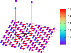
Figure 1: Scheme of the lattice model with three additional sites (”adatoms”). Red lines represent hoppings, Kekule pattern is shown with bold and thin lines. Bold ones correspond to larger hopping $t=1.3$ and the thin lines correspond to smaller hopping $t=1.0$. Hoppings to additional sites are equal to $t^{\prime}=10.0$. Black lines connect the sites involved in charge-charge interactions. Color scale corresponds to the modulus of the Wannier wavefunction, concentrated around one of the adatoms.

I.2 Projection method

We start from the diagonalization of the free Hamiltonian $\hat{H}_{K}$, which gives us $N_{L}$ states in lower (valence) band, $N_{U}$ states in upper (conduction) band and $N_{0}$ states in the flat band, where $N_{0}$ is equal to the number of adatoms. We introduce the field operators for these states

$$\hat{\psi}_{i,\sigma}=\sum_{x}\psi_{i}(x)\hat{a}_{x,\sigma},$$ (3)

where $\psi_{i}(x)$ is the single-electron wavefunction of the $i$-th eigenvalue of the free Hamiltonian $\hat{H}_{K}$, including both upper, lower, and flat band. In the case of degenerate energy levels inside the flat band, we choose maximally localized Wannier functions Marzari et al. (2012). Example of one such wave function, localized near one of the adatoms, is shown in Fig. 1 using the color of the lattice sites.

Using this single-particle basis, a general vector in the Hilbert space for 3-band system can be written as follows:

$$|\Psi\rangle=|n^{L}_{1,\sigma},n^{L}_{2,\sigma}...n^{L}_{N_{L},\sigma};n^{0}_{1,\sigma}...n^{0}_{N_{0},\sigma};n^{U}_{1,\sigma},...n^{U}_{N_{U},\sigma}\rangle.$$ (4)

$\{n^{U}\}$, $\{n^{L}\}$ and $\{n^{0}\}$ are occupation numbers (eigenvalues of the particle number operators $\hat{\psi}^{\dagger}_{i,\sigma}\hat{\psi}_{i,\sigma}$) for both spin projections for energy levels in upper, lower and flat band correspondingly. Of course, the system can have more than 3 bands, but for simplicity we joined all bands below the flat band in one ”lower” band and all bands above the flat band in the ”upper” one.

Since the flat band is energetically separated from upper and lower bands (we will give a numerical estimation for the degree of separation needed below), we develop the effective theory for the flat band by projecting into the subspace $\mathcal{P}$, where the lower band is completely filled and the upper band is empty.

$$|\Psi_{P}\rangle=\hat{P}|\Psi\rangle=|1,...1;n^{0}_{1,\sigma}...n^{0}_{N_{0},\sigma};0,...0\rangle.$$ (5)

We stress that the symmetries of the original model such as global spin and charge invariance carry over to the effective model defined in the projected Hilbert space.

A general expression for the effective Hamiltonian inside the projected subspace is written as follows:

$$\hat{H}_{eff.}(E)=\hat{P}\hat{H}\hat{P}+\hat{P}\hat{H}\hat{R}\frac{1}{E-\hat{R}\hat{H}\hat{R}}\hat{R}\hat{H}\hat{P},$$ (6)

where $\hat{H}=\hat{H}_{K}+\hat{H}_{U}$, $\hat{R}=I-\hat{P}$, and $E$ is the energy. This expression can be derived e.g. using the Schur complement starting from the equation for the eigenvalues of the initial Hamiltonian in the full Hilbert space:

$$\det(\hat{H}-E)=\det\begin{pmatrix}\hat{P}\hat{H}\hat{P}-E&\hat{P}\hat{H}\hat{R}\\ \hat{R}\hat{H}\hat{P}&\hat{R}\hat{H}\hat{R}-E\end{pmatrix}=$$

$$\det(\hat{R}\hat{H}\hat{R}-E)$$ (7)

$$\times\det(P\hat{H}\hat{P}-E-\hat{P}\hat{H}\hat{R}\frac{1}{\hat{R}\hat{H}\hat{R}-E}\hat{R}\hat{H}\hat{P}).$$

Since the system features a gap, the desired subspace with dynamics concentrated in the flat band only forms a low energy sector of the full set of eigenvalues. Thus we can assume that the term $\det(\hat{R}\hat{H}\hat{R}-E)$, which features the projection outside of the $\mathcal{P}$ subspace never vanishes. Hence we can consider only the second term, leading exactly to the expression 6.

Since the expression for the effective Hamiltonian includes the energy, we will need to solve the equation for the eigenvalues

$$\det\left({H_{eff}}_{ij}(E)-\delta_{ij}E\right)=0$$ (8)

self-consistently including the dependence on energy inside the matrix of the effective Hamiltonian ${H_{eff}}_{ij}(E)$.

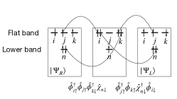
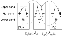
Figure 2: Examples of diagrams for matrix elements $\langle\Psi_{L}|\hat{H}_{eff}|\Psi_{R}\rangle$, following from the second term in 17 under the assumption that only diagonal operators in the basis 4 are left in the denominator. Diagram (a) corresponds to some particular terms in $\hat{V}^{(1,1)}$ and $\hat{V}^{(1,2)}$; (b) corresponds to $\hat{V}^{(2,1)}$; (c) corresponds to $\hat{V}^{(3,1)}$ and $\hat{V}^{(3,2)}$. Operator terms shown in the diagrams are written below the arrows which indicate the transitions caused by these terms.

Now, we rewrite the effective Hamiltonian 6 using the field operators 3. First, we separate the part of Hamiltonian which can not transfer the states outside subspace $\mathcal{P}$:

$$\hat{H}=\hat{H}_{\phi}+\hat{V},$$ (9)

$$\hat{P}\hat{H}_{\phi}\hat{R}=0.$$ (10)

For simplicity, we will denote the field operators for the flat band modes as $\hat{\phi}_{i,\sigma}$, and field operators for upper and lower bands as $\hat{\chi}_{i,\sigma}$. Thus the operator $\hat{H}_{\phi}$ in 9 can be written in the following general form

$$\hat{H}_{\phi}=\sum_{ijkn}H^{(1)}_{ijkn}\hat{\phi}^{\dagger}_{i,\sigma}\hat{\phi}_{j,\sigma}\hat{\phi}^{\dagger}_{k,\sigma^{\prime}}\hat{\phi}_{n,\sigma^{\prime}}+\sum_{ij}H^{(2)}_{ij}\hat{\phi}^{\dagger}_{i,\sigma}\hat{\phi}_{j,\sigma}$$

$$+\sum_{ijk}H^{(3)}_{ijk}\hat{\phi}^{\dagger}_{i,\sigma}\hat{\phi}_{j,\sigma}\hat{\chi}^{\dagger}_{k,\sigma^{\prime}}\hat{\chi}_{k,\sigma^{\prime}}+\sum_{i}H^{(4)}_{i}\hat{\chi}^{\dagger}_{i,\sigma}\hat{\chi}_{i,\sigma}$$ (11)

$$+\sum_{ij}H^{(5)}_{ij}\hat{\chi}^{\dagger}_{i,\sigma}\hat{\chi}_{i,\sigma}\hat{\chi}^{\dagger}_{j,\sigma^{\prime}}\hat{\chi}_{j,\sigma^{\prime}}.$$

As in 1, summation over spin indexes is implied. $H^{(i)}$ coefficients can be easily computed after substitution of the field operators 3 in Hamiltonian $\hat{H}$. For example,

$$H^{(1)}_{ijkn}=\frac{1}{2}\sum_{x,y}U_{x,y}\left(\phi_{i}(y)\phi^{*}_{j}(y)\phi_{k}(x)\phi^{*}_{n}(x)\right.$$

$$+\left.\phi_{i}(x)\phi^{*}_{j}(x)\phi_{k}(y)\phi^{*}_{n}(y)\right)$$ (12)

$\hat{H}_{\phi}$ is constructed using the principle, that any expression involving $\hat{\chi}$ operators allowed in it should consist only from particle number operators $\hat{n}^{(\chi)}_{i,\sigma}=\hat{\chi}^{\dagger}_{i,\sigma}\hat{\chi}_{i,\sigma}$ in various combinations. Thus $\hat{H}_{\phi}$ can be further simplified, since $\hat{P}$ $\chi^{\dagger}_{i,\sigma}\hat{\chi}_{j,\sigma^{\prime}}=\delta_{i,j}\delta_{\sigma,\sigma^{\prime}}\epsilon$ with $\epsilon=0,1$ and all particle number operators $\hat{n}^{(\chi)}_{i,\sigma}$ can be simply substituted by corresponding occupation numbers. Examples of $\hat{H}_{\phi}$ include effective models for twisted bilayer graphene Bistritzer and MacDonald (2011); Khalaf et al. (2021); Hofmann et al. (2022); Zhang et al. (2023) as well as landau level projections Wang et al. (2021); Zhu et al. (2023). Here we go beyond this approximation and include corrections occurring from the high energy bands.

The operator $\hat{V}$ contains all remaining terms in the Hamiltonian $\hat{H}$:

$$\hat{V} = \hat{V}^{(1)}+\hat{V}^{(2)}+\hat{V}^{(3)}$$

$$+ \sum_{i\neq j,k\neq n}V^{(4)}_{ijkn}\hat{\chi}^{\dagger}_{i,\sigma}\hat{\chi}_{j,\sigma}\hat{\chi}^{\dagger}_{k,\sigma^{\prime}}\hat{\chi}_{n,\sigma^{\prime}}+\sum_{i\neq j}V^{(5)}_{ij}\hat{\chi}^{\dagger}_{i,\sigma}\hat{\chi}_{j,\sigma}$$

where $\hat{V}^{i},i=1,2,3$ operators correspond to the i-particle excitations to upper (lower) band:

$$\hat{V}^{(1)}=\sum_{ijkn}V^{(1,1)}_{ijkn}\hat{\phi}^{\dagger}_{i,\sigma}\hat{\phi}_{j,\sigma}\hat{\phi}^{\dagger}_{k,\sigma^{\prime}}\hat{\chi}_{n,\sigma^{\prime}}+$$

$$\sum_{ijkn}V^{(1,2)}_{ijkn}\hat{\phi}^{\dagger}_{i,\sigma}\hat{\phi}_{j,\sigma}\hat{\chi}^{\dagger}_{k,\sigma^{\prime}}\hat{\phi}_{n,\sigma^{\prime}}+$$ (14)

$$+\sum_{ij}V^{(1,3)}_{ij}\hat{\phi}^{\dagger}_{i,\sigma}\hat{\chi}_{j,\sigma}+\sum_{ij}V^{(1,4)}_{ij}\hat{\chi}^{\dagger}_{i,\sigma}\hat{\phi}_{j,\sigma}$$

$$+\sum_{ijk}V^{(1,5)}_{ijkn}\hat{\phi}^{\dagger}_{i,\sigma}\hat{\chi}_{j,\sigma}\hat{\chi}^{\dagger}_{k,\sigma^{\prime}}\hat{\chi}_{k,\sigma^{\prime}}$$

$$+\sum_{ijk}V^{(1,6)}_{ijkn}\hat{\chi}^{\dagger}_{i,\sigma}\hat{\phi}_{j,\sigma}\hat{\chi}^{\dagger}_{k,\sigma^{\prime}}\hat{\chi}_{k,\sigma^{\prime}}$$

$$\hat{V}^{(2)}=\sum_{ij,k\neq n}V^{(2,1)}_{ij,kn}\hat{\phi}^{\dagger}_{i,\sigma}\hat{\phi}_{j,\sigma}\hat{\chi}^{\dagger}_{k,\sigma^{\prime}}\hat{\chi}_{n,\sigma^{\prime}}+$$

$$\sum_{ijkn}V^{(2,2)}_{ijkn}\hat{\phi}^{\dagger}_{i,\sigma}\hat{\chi}_{j,\sigma}\hat{\phi}^{\dagger}_{k,\sigma^{\prime}}\hat{\chi}_{n,\sigma^{\prime}}+$$

$$\sum_{ijkn}V^{(2,3)}_{ijkn}\hat{\chi}^{\dagger}_{i,\sigma}\hat{\phi}_{j,\sigma}\hat{\chi}^{\dagger}_{k,\sigma^{\prime}}\hat{\phi}_{n,\sigma^{\prime}}+$$ (15)

$$\sum_{ijkn}V^{(2,4)}_{ijkn}\hat{\phi}^{\dagger}_{i,\sigma}\hat{\chi}_{j,\sigma}\hat{\chi}^{\dagger}_{k,\sigma^{\prime}}\hat{\phi}_{n,\sigma^{\prime}}$$

$$\hat{V}^{(3)}=\sum_{i\neq j,kn}V^{(3,1)}_{ijkn}\hat{\chi}^{\dagger}_{i,\sigma}\hat{\chi}_{j,\sigma}\hat{\chi}^{\dagger}_{k,\sigma^{\prime}}\hat{\phi}_{n,\sigma^{\prime}}+$$

$$\sum_{i\neq j,kn}V^{(3,2)}_{ijkn}\hat{\chi}^{\dagger}_{i,\sigma}\hat{\chi}_{j,\sigma}\hat{\phi}^{\dagger}_{k,\sigma^{\prime}}\hat{\chi}_{n,\sigma^{\prime}}$$ (16)

Coefficients $V^{(i)}$ again can be easily obtained after applying the transformation 3 to $\hat{a}_{x,\sigma}$ operators in $\hat{H}$.

Now, the effective Hamiltonian 6 can be rewritten as

$$\hat{H}_{eff.}(E)=\hat{H}_{\phi}+\hat{P}\hat{V}\hat{R}\frac{1}{E-\hat{R}(\hat{H}_{\phi}+\hat{V})\hat{R}}\hat{R}\hat{V}\hat{P}.$$ (17)

This expression still gives exact values of energy, since no approximations were made. However, the second term includes the inversion of the interaction Hamiltonian $\hat{V}$, thus it can not be evaluated exactly. Starting from this point we make the approximations assuming that the gap in one particle spectrum between upper and lower band is larger than matrix elements of the interaction Hamiltonian. The intermediate states $|\Psi_{I}\rangle=\hat{R}\hat{V}\hat{P}|\Psi\rangle$ in the second term in 17 have at least one excitation in upper or lower band. Thus, the denominator in 17 is dominated by the kinetic energy of these excitations given by

$$\hat{H}^{(4)}=\sum_{i}H^{(4)}_{i}\hat{\chi}^{\dagger}_{i,\sigma}\hat{\chi}_{i,\sigma}$$ (18)

term in $\hat{H}_{\phi}$ Hamiltonian, with all other terms only giving subleading contributions. In addition to the large kinetic term, we also assume the presence of relatively large Hubbard-type interactions, leading to the localization of the states especially in the flat band. Consequently, we retain additional terms in the denominator of 17. These are essentially all terms, which are diagonal in the basis 4. In the end the following operators are left in the denominator: $\hat{H}^{(4)},\,\hat{H}^{(5)},\hat{\tilde{H}}^{(1)},\hat{\tilde{H}}^{(2)},\hat{\tilde{H}}^{(3)}$. $\hat{H}^{(4)}$ is defined in 18. The remaining four operators are defined as

$$\hat{H}^{(5)}=\sum_{ij}H^{(5)}_{ij}\hat{\chi}^{\dagger}_{i,\sigma}\hat{\chi}_{i,\sigma}\hat{\chi}^{\dagger}_{j,\sigma^{\prime}}\hat{\chi}_{j,\sigma^{\prime}}.$$

$$\hat{\tilde{H}}^{(1)}=\sum_{ij}H^{(1)}_{iijj}\hat{\phi}^{\dagger}_{i,\sigma}\hat{\phi}_{i,\sigma}\hat{\phi}^{\dagger}_{j,\sigma^{\prime}}\hat{\phi}_{j,\sigma^{\prime}},$$

$$\hat{\tilde{H}}^{(2)}=\sum_{i}H^{(2)}_{ii}\hat{\phi}^{\dagger}_{i,\sigma}\hat{\phi}_{i,\sigma},$$ (19)

$$\hat{\tilde{H}}^{(3)}=\sum_{ik}H^{(3)}_{iik}\hat{\phi}^{\dagger}_{i,\sigma}\hat{\phi}_{i,\sigma}\hat{\chi}^{\dagger}_{k,\sigma^{\prime}}\hat{\chi}_{k,\sigma^{\prime}}.$$

Under these assumptions, all terms in $\hat{V}^{(i)}$ operators can be depicted as parts of diagrams for the matrix elements of $\hat{H}_{eff.}$. Examples of such diagrams are shown in Fig. 2. In practice, all these diagrams are generated automatically by the projection code.

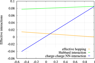
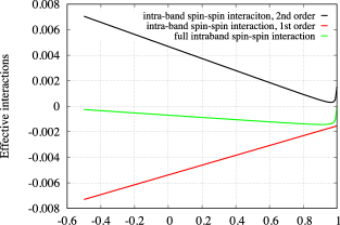
Figure 3: Effective interactions for two electrons in the flat band, computed from intra-band term $\hat{H}_{\phi}$ within the second order perturbation theory. (a) effective hopping $t_{eff.}$ (see 34); effective Hubbard interaction $U_{eff.}$ (see 26) and full effective charge-charge interaction $V_{eff.}+\frac{1}{2}J^{(1)}_{eff.}$ (see 28). (b) Effective spin-spin interaction within the 1st ($J^{(1)}_{eff.}$, see 31) and the 2nd order ($J^{(2)}_{eff.}$, see 33) perturbation theory, as well as their sum $J^{(2)}_{eff.}+J^{(2)}_{eff.}$. Calculation were done for the system described in the figure 1 with the matrix of interactions defined in 22. $U_{0}=1.0$.

In order to further simplify the calculations, we take into account only single-particle excitations, described by $\hat{V}^{(1)}$ operator when writing the nominator of the second term in 17. Many-particle excitations in the intermediate state $|\Psi_{I}\rangle$ in the second term in 17 have larger energy described by the term $\langle\Psi_{I}|\hat{H}^{(4)}|\Psi_{I}\rangle$ again due to the presence of a large mass gap in the system. Thus, these excitations are again suppressed by the mass gap.

The final expression for the effective Hamiltonian can be written as

$$\hat{H}_{eff.}(E)\approx\hat{H}_{\phi}+\hat{P}\hat{V}^{(1)}\hat{R}\frac{1}{E-\hat{R}\hat{\tilde{H}}_{\phi}\hat{R}}\hat{R}\hat{V}^{(1)}\hat{P},$$ (20)

where

$$\hat{\tilde{H}}_{\phi}=\hat{\tilde{H}}^{(1)}+\hat{\tilde{H}}^{(2)}+\hat{\tilde{H}}^{(3)}+\hat{H}^{(4)}+\hat{H}^{(5)}$$ (21)

is the part of $\hat{\tilde{H}}_{\phi}$ operator, diagonal in the basis 4.

Subsequently, we construct the matrix of the Hamiltonian $\hat{H}_{eff.}$ in the subspace 5 taking into account all possible single electron (hole) excitations in the intermediate state. After construction of this matrix, the eigenvalues are found using Eq. 8.

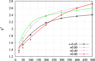
Figure 4: (a) Scheme of the lowest energy levels of the approximate effective Hamiltonian from eq. 20 for the system described in the figure 1 leading to the $\bar{S}(\beta)$ function 37 used for the fitting in the figure (b). Narrow band is depicted by a rectangle, two degenerate states are depicted as double line. Trivial $M_{z}$ degeneracy of the spin states is not shown on the scheme. (b)Temperature profiles of $\langle\hat{S}^{2}\rangle$ from QMC data and their fitting with two-exponents function $\bar{S}(\beta)$ 37. Calculations were done for the system described in the figure 1 with the matrix of interactions defined in 22. $U_{0}=0.5$.

I.3 Approximate solution for intra-band terms of effective Hamiltonian

The two terms in the effective Hamiltonian of Eq.20 can be considered separately. The first term does not contain any excitations to the upper or lower bands, thus we collectively call all terms in $\hat{H}_{\phi}$ as ”intra-band”. The second term in 20 contains excitations to upper and lower band, thus we call all terms within it as ”exchange terms”. Before moving to the exact diagonalization of the approximate effective Hamiltonian 20, we consider a perturbative approach to provide simplified approximate expressions of the effective interactions between electrons inside the flat band. Namely, we concentrate on $\hat{H}_{\phi}$ Hamiltonian (”intra-band” terms) only, and develop the separate perturbation theory for it assuming that the overlap between Wannier functions concentrated near different adatoms is small.

In order to provide an explicit example, we consider a system of three adatoms depicted in Fig. 1. The interaction Hamiltonian includes three sites of the Honeycomb lattice at which the amplitudes of the corresponding Wannier functions are maximal. With this arrangement, the matrix of interactions includes just these three sites and is written as

$$U=U_{0}\begin{pmatrix}1&\alpha&\alpha\\ \alpha&1&\alpha\\ \alpha&\alpha&1\end{pmatrix}.$$ (22)

The parameter $\alpha$ changes the ratio between on-site and long-range interactions. The matrix $U$ is positive definite provided that $\alpha\in[-1/2;1]$, and only this interval is accessible to QMC simulations. The full Hamiltonian $\hat{H}=\hat{H}_{K}+\hat{H}_{U}$ thus reads as

$$\hat{H}=\hat{H}_{K}+\frac{1}{2}\sum_{i,j=1}^{3}U_{i,j}\hat{q}_{i}\hat{q}_{j}$$ (23)

with $\hat{q}_{i}=\sum_{\sigma}(\hat{a}^{\dagger}_{i,\sigma}\hat{a}^{\phantom{\dagger}}_{i,\sigma}-1/2)$. The position of the adatoms and the values of hoppings are given in Fig. 1.

For the model of Eq. 23 $\hat{H}_{\phi}$ is constructed with 11. Terms proportional to $H^{(i)},i\neq 1$ give only two-fermionic terms for the flat band operators $\hat{\phi}_{i,\sigma}$. These terms corresponds to a chemical potential for the flat band and ensure half-filling. Non trivial electron-electron correlations stem from the four-fermionic terms proportional to $H^{(1)}_{ijkn}$. A hierarchy in these terms emerges by assuming that the overlap between different Wannier functions inside the flat band is small. This assumption can be formalized in the following relations between the coefficients $H^{(1)}_{ijkn}$

$$|H^{(1)}_{iiii}|>|H^{(1)}_{iijj}|\gg|H^{(1)}_{ijji}|,\,|H^{(1)}_{iiij}|$$

$$\gg|H^{(1)}_{ikkj}|\gg|H^{(1)}_{ijkn}|,i\neq j\neq k\neq n$$ (24)

This implies that the dominant term in the expression 11 for $\hat{H}_{\phi}$ is the effective Hubbard interaction

$$\hat{H}^{(H)}_{eff.}=\sum_{i}U_{eff.}\hat{\phi}^{\dagger}_{i,\uparrow}\hat{\phi}_{i,\uparrow}\hat{\phi}^{\dagger}_{j,\downarrow}\hat{\phi}_{j,\downarrow},$$ (25)

where

$$U_{eff.}=H^{(1)}_{iiii},\quad\forall i.$$ (26)

In general, $U_{eff.}$ should be dependent on the index of corresponding Wannier wave function. However, all three adatoms are equivalent in our case, so that $U_{eff.}$ does not depend on the choice of particular state in the flat band. Thus, for simplicity, we drop the $i$ index on the left hand side of the expression 26.

As mentioned previously, global SU(2) spin and U(1) charge symmetries are conserved in the projected Hilbert space, spanned by the states $|\Psi_{P}\rangle$ (see Eq. 5). Hence we can use the third component of total spin $M_{z}$ and total number of particles to classify the eigenstates. These symmetries together with the dominance of the effective Hubbard interaction 26 ensure that the ground state belongs to the subspace corresponding to half filled flat band with three electrons in it. It is also enough to only consider $M_{z}=1/2$.

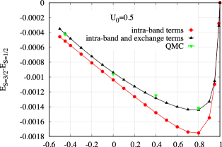
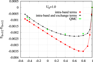
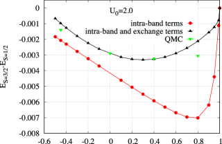
Figure 5: Energy gap between $S=3/2$ and $S=1/2$ states in the subspace with three electrons in the flat band for the system shown in the figure 1. Matrix of interactions is defined in 22. Intra-band terms correspond to the diagonalization of $\hat{H}_{\phi}$ in 20. In the case of exchange terms, only single electron (hole) excitations are taken into account (see the second term in 20).

The next term in the hierarchy of four-fermionic terms in $\hat{H}_{\phi}$ is the effective charge-charge interaction.

$$\hat{H}^{Q}_{eff.}=\frac{1}{2}V_{eff.}\sum_{i\neq j}\hat{Q}_{i}\hat{Q}_{j},$$ (27)

where

$$V_{eff.}=H^{(1)}_{iijj},\quad\forall i\neq j.$$ (28)

$\hat{Q}_{i}=\hat{\phi}^{\dagger}_{i,\uparrow}\hat{\phi}_{i,\uparrow}+\hat{\phi}^{\dagger}_{i,\downarrow}\hat{\phi}_{i,\downarrow}-1$ is the charge operator for the electron in the flat band at the i-th state.

Both $\hat{H}^{Q}_{eff.}$ and $\hat{H}^{H}_{eff.}$ are diagonal in the basis 5. Thus, according to the assumption 24 we can use them as the zeroth order term in the perturbation theory for $\hat{H}_{\phi}$:

$$\hat{H}^{(0)}_{eff.}=\frac{1}{2}U_{eff.}\sum_{i}\hat{Q}^{2}_{i}+\frac{1}{2}V_{eff.}\sum_{i\neq j}\hat{Q}_{i}\hat{Q}_{j}.$$ (29)

Since typically $U_{eff.}>V_{eff.}$, the zeroth order of perturbation theory results in fully localized electrons inside the flat band.

All other terms in $\hat{H}_{\phi}$ are considered as a perturbation in comparison to 29. In the first order perturbation theory, only terms proportional to $H^{(1)}_{ijji}$ contribute and we obtain an effective spin-spin and additional charge-charge interactions between electrons in the flat band:

$$\hat{H}^{(1)}_{eff.}=J^{(1)}_{eff.}\sum_{i\neq j}\left(2\hat{\vec{S}}_{i}\hat{\vec{S}}_{j}+\frac{1}{2}\hat{Q}_{i}\hat{Q}_{j}\right),$$ (30)

where

$$J^{(1)}_{eff.}=-H^{(1)}_{ijji},\quad\forall i\neq j$$ (31)

At second order, we obtain additional spin-spin interactions

$$\hat{H}^{(2)}_{eff.}=J^{(2)}_{eff.}\sum_{i\neq j}\left(2\hat{\vec{S}}_{i}\hat{\vec{S}}_{j}\right),$$ (32)

where

$$J^{(2)}_{eff.}=\frac{|H^{(1)}_{iiij}-H^{(1)}_{jjji}|^{2}+\sum_{k\neq i,j}|H^{(1)}_{ikkj}|^{2}}{U_{eff.}-(V_{eff.}+\frac{1}{2}J^{(1)}_{eff.})}\quad\forall i\neq j.$$ (33)

This term is similar to the expression we obtain for the effective Heisenberg model in terms of a strong-coupling expansion of the Hubbard model. Due to this analogy, we can introduce an effective hopping, induced by interactions inside the flat band:

$$t_{eff.}=\sqrt{|H^{(1)}_{iiij}-H^{(1)}_{jjji}|^{2}+\sum_{k\neq i,j}|H^{(1)}_{ikkj}|^{2}},\quad\forall i\neq j.$$ (34)

Dependencies of the effective interactions on $\alpha$ for $U_{0}=1$ are shown in the Fig.3 for the system described in Fig.  1. We plot the effective Hubbard interaction $U_{eff.}$, full effective charge-charge interaction $V_{eff.}+\frac{1}{2}J^{(1)}_{eff.}$, and the first and the second order spin-spin interactions $J^{(1)}_{eff.}$ and $J^{(2)}_{eff.}$ separately.

As one can see, the Hubbard interaction is indeed dominant for most of the considered values of $\alpha$, except for the region around $\alpha=1$, where the nearest-neighbour charge-charge interaction competes with Hubbard interaction. Thus the perturbation theory for intra-band terms is justified everywhere except the vicinity of the $\alpha=1$ point. Comparison of $J^{(1)}_{eff.}$ and $J^{(2)}_{eff.}$ shows that non-frustrated negative $J^{(1)}_{eff.}$ interaction dominates over frustrated positive $J^{(2)}_{eff.}$ interaction everywhere within the region accessible to QMC simulations: $\alpha\in[-1/2;1]$. Of course, this is only a very preliminary result, which only takes into account intra-band terms, and relies on perturbation theory. However, this picture will be justified later for the complete exact diagonalization of the approximate effective Hamiltonian 20 including exchange terms.

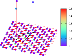
Figure 6: Scheme of the lattice model with three additional sites (”adatoms”) and alternative setup for interaction Hamiltonian 2. Red lines represent hoppings, Kekule pattern is shown with bold and thin lines. Bold ones correspond to larger hopping $t=1.3$ and the thin lines correspond to smaller hopping $t=1.0$. Hoppings to additional sites are equal to $t^{\prime}=10.0$. Black lines connect the sites involved in charge-charge interactions. Color scale corresponds to the modulus of the Wannier wavefunction, concentrated around one of the additional sites.

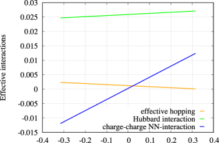
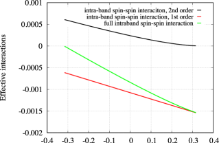
Figure 7: Effective interactions for two electrons in the flat band, computed from intra-band term $\hat{H}_{\phi}$ within the second order perturbation theory for the system described in the figure 6. (a) effective hopping $t_{eff.}$ (see 34); effective Hubbard interaction $U_{eff.}$ (see 26) and full effective charge-charge interaction $V_{eff.}+\frac{1}{2}J^{(1)}_{eff.}$ (see 28). (b) Effective spin-spin interaction within the 1st ($J^{(1)}_{eff.}$, see 31) and the 2nd order ($J^{(2)}_{eff.}$, see 33) perturbation theory, as well as their sum $J^{(2)}_{eff.}+J^{(2)}_{eff.}$. Calculation were done with the matrix of interactions defined in 41. $U_{0}=1.0$.

II QMC verification of the projection algorithm

In order to estimate the quality of the approximations made during the derivation of the effective Hamiltonian 20 a verification is made via comparison to unbiased QMC simulations carried out for parameters of the model, where the sign problem is absent. For this verification, we switch to the exact diagonalization of the approximate effective Hamiltonian 20, including both intra-band and exchange terms.

Auxiliary-field QMC simulations were carried out with the ALF Assaad et al. (2022) implementation of the finite temperature auxiliary field QMC algorithm Blankenbecler et al. (1981); White et al. (1989); Assaad and Evertz (2008). We consider the system depicted in Fig. 1 with electron-electron interaction defined in 22 and Hamiltonian of Eq. 23. In order to decouple the charge-charge interactions we first rewrite them as the perfect square of one body terms. Depending on the sign of the parameter $\alpha$ we employ different decouplings to prevent the occurrence of the sign problem. For $\alpha$ in the interval $[-1/2;0]$ we write

$$\hat{H}_{U}=U_{0}\left(\frac{1}{2}+\alpha\right)\sum_{i=1}^{3}\hat{q}_{i}^{2}-\frac{\alpha}{2}U_{0}\sum_{i>j}(\hat{q}_{i}-\hat{q}_{j})^{2}$$ (35)

and for $\alpha\in]0;1]$

$$\hat{H}_{U}=\frac{1}{2}U_{0}(1-\alpha)\sum_{i=1}^{3}\hat{q}_{i}^{2}+\frac{\alpha}{2}U_{0}\left(\sum_{i=1}^{3}\hat{q}_{i}\right)^{2}.$$ (36)

Here the sum over $i$ and $j$ goes over the three interacting sites depicted in Fig. 1. After this we can perform a Trotter decomposition and a discrete Hubbard-Stratonovich (HS) decomposition as outlined in Ref. Assaad et al. (2022). The Trotter step size was fixed to $\Delta\tau=0.1t$ for all simulations. Lattice size corresponds exactly to Fig.  1, with periodical boundary conditions in all directions.

Since the (non-)appearance of the frustrated ground state is the most interesting physical effect in this system, we compute the energy difference between the states with $S=3/2$ and $S=1/2$ inside the subspace with 3 electrons in the flat band. This energy difference roughly corresponds to the effective spin-spin interaction between electrons localized around different adatoms, and we use it to compare the QMC data with the exact diagonalization of approximate effective Hamiltonian.

In order to extract this difference from QMC data, we plot the temperature dependence of average squared spin $\bar{S}=\langle\hat{\vec{S}}^{2}\rangle$ and fit it to the form:

$$\bar{S}(\beta)=\frac{9e^{-\Delta E_{2}\beta}+3e^{-\Delta E_{1}\beta}+15}{12e^{-\Delta E_{2}\beta}+4e^{-\Delta E_{1}\beta}+4},$$ (37)

where $\beta$ is the inverse temperature. Here $\vec{S}=\frac{1}{2}\sum_{x\in\mathcal{H,A},s,s^{\prime}}a^{\dagger}_{x,s}\vec{\sigma}_{s,s^{\prime}}a^{\phantom{\dagger}}_{x,s^{\prime}}$ corresponds to the total spin.

This fitting form takes into account all states within the subspace with three electrons in the flat band, which is the lowest subspace in the energy spectrum of the whole system. Namely, the fitting form accounts for one (four-fold degenerate) $S=3/2$ state with energy $E_{S=3/2}$, two (two-fold degenerate) $S=1/2$ states with identical energy $E_{S=1/2}$ and six remaining delocalized two-fold degenerate states with $S=1/2$. The latter states are not completely degenerate and form a narrow band, but for simplicity we assume that they are characterized by the same energy $E^{\prime}_{S=1/2}$. Thus the parameters of the fitting form 37 are defined as

$$\Delta E_{1}=E_{S=1/2}-E_{S=3/2},$$ (38)

$$\Delta E_{2}=E^{\prime}_{S=1/2}-E_{S=3/2}.$$ (39)

The energy levels are shown in Fig. 4. Examples of such fits for different values of $\alpha$ are shown in Fig. 4. There are some deviations at low $\beta$, which correspond to the participation of higher energy levels in the $\bar{S}(\beta)$ profiles. However, at $\beta>200$ the fitting curves are indistinguishable from the QMC data.

The energy differences $\Delta E_{1}$ extracted from the fits are compared with the same differences obtained from exact diagonalization of the approximate effective Hamiltonian 20. For the latter dataset, we show two points for each $\alpha$: one point corresponds to the exact diagonalization of intra-band terms $\hat{H}_{\phi}$ only (an exact version of the approximate calculation from Sec. I.3); and another point corresponds to complete Hamiltonian $\hat{H}_{eff.}$. Difference between these two points show the role of exchange terms. Results are shown in Fig.5 for three values of $U_{0}=0.5,1.0,2.0$. As expected from the approximations based on the assumption of a large gap, the effective Hamiltonian performs well for smaller $U=0.5,1.0$, but some noticeable deviations appear at $U=2.0$. However, the approximation never causes a qualitative error: QMC shows that everywhere inside the interval $\alpha\in[-1/2;1]$ accessible for the simulations we get non-frustrated $S=3/2$ ground state, and the same is true for the exact diagonalization of approximate effective Hamiltonian. In general, the comparison shows that it is safe to use the approximate Hamiltonian up to $U/m\simeq 3$, where $m$ is the gap between upper and lower bands.

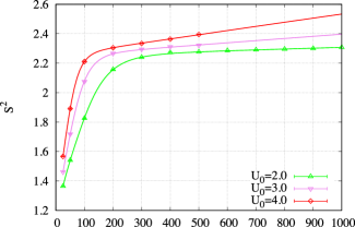
Figure 8: (a) Scheme of the lowest energy levels of the approximate effective Hamiltonian from eq. 20 for the system described in the figure 6 leading to the $\bar{S}(\beta)$ function 42 used for the fitting in the figure (b). Narrow bands are depicted by rectangles, two degenerate states are depicted as double line. Trivial $M_{z}$ degeneracy of the spin states is not shown on the scheme. (b)Temperature profiles of $\langle\hat{S}^{2}\rangle$ from QMC data and their fitting with the four-exponents function $\bar{S}(\beta)$ 42. Calculations were done for the system described in the figure 6 for the interaction Hamiltonian 40 at $\alpha=-\sqrt{1/10}$.

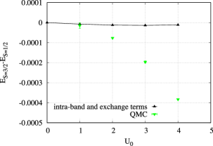
Figure 9: Energy gap between $S=3/2$ and $S=1/2$ states within the subspace with three electrons in the flat band. Calculations were done for the system shown in the figure 6 with the interaction matrix defined in 41 at $\alpha=-\sqrt{1/10}$. Intra-band and exchange terms correspond to the diagonalization of the approximate effective Hamiltonian 20. QMC data is the result of the fitting procedure, shown in the figure 8.

III Mapping of the sign problem for spin frustrated system

Now the question is, whether we can generate an effective model with frustrated spin interactions within the flat band, while still preserving the possibility to perform QMC simulations of the whole lattice model. Unfortunately, attempts of numerical optimization of the lattice model show that the answer is negative. However, it is possible to generate an effective model with frustrated spins if we consider the microscopic interaction Hamiltonian 2 with mixture of positive and negative eigenvalues in the matrix $U$. Such models provide a mapping from the sign problem for spin frustrated system to the problem of different signs of eigenvalues of interaction matrix.

III.1 Zero spin-spin interaction at the edge of the parameters’ region accessible for QMC

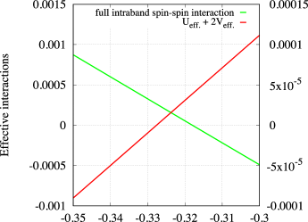
Figure 10: Flat band spin-spin interaction and $U_{eff.}+2V_{eff.}$ interaction for the system depicted in the figure 6 beyond the critical $\alpha=-\sqrt{1/10}$ value. Left scale corresponds to $U_{eff.}+2V_{eff.}$ interaction, right scale corresponds to the spin-spin interaction. Calculations were done for intra-band terms in 20, using the second order perturbation theory (see eq. 31 and 33 for spin-spin interaction and eq. 26, 28 for charge-charge interaction). Matrix of interactions is defined in 40, 41; $U_{0}$=1.0.

First, we perform a numerical optimization of the $U$ matrix trying to maximize full intra-band spin-spin interaction $J^{(\Sigma)}_{eff.}=J^{(1)}_{eff.}+J^{(2)}_{eff.}$. This quantity is rather cheap to compute, thus the optimization can be performed efficiently. However, it seems that we can not make $J^{(\Sigma)}_{eff.}$ positive keeping all eigenvalues of $U$ matrix also positive. The maximum which we can obtain is the situation when one (or several) eigenvalues of the U matrix are zero, others are positive and the full intra-band spin-spin interaction is zero. Such a system is shown in Fig. 6. The interaction consists of three dimer terms, and six different sites are included. These sites are shown in the Fig. 6 connected by black lines. We denote charge operators at these sites as $\hat{q}^{j}_{i}$, where $i=1,2,3$ is index of a dimer and $j=1,2$ is index of a site in the dimer $i$. $\hat{q}^{1}_{i}$ always corresponds to the site, which is the nearest neighbour to the one with an adatom attached to it (see Fig. 6). The whole interaction Hamiltonian is written as

$$\hat{H}_{U}=\sum^{3}_{i=1}\frac{1}{2}\sum^{2}_{n,m=1}U_{nm}\hat{q}^{n}_{i}\hat{q}^{m}_{i},$$ (40)

where the $2\times 2$ matrix $U$ is defined as

$$U=U_{0}\begin{pmatrix}0.1&\alpha\\ \alpha&1\end{pmatrix}$$ (41)

Both eigenvalues of $U$ matrix are positive if $\alpha\in[-\sqrt{1/10};\sqrt{1/10}]$.

Full $\alpha$ profiles of effective interactions obtained via the 2-nd order perturbation theory for intra-band part of the effective Hamiltonian are shown in the Fig. 7. As one can see, $J^{(\Sigma)}_{eff.}$ is exactly zero at the left edge of the allowed interval for $\alpha$.

In a second step, we check if the inter-band terms renormalize the effective spin-spin interaction towards frustrated or non-frustrated regime. In addition to that, we again perform QMC simulations at $\alpha=-\sqrt{1/10}$ in order to provide an independent control to the results of the exact diagonalization of the approximate effective Hamiltonian . At this stage we use the routine already described in Sec. II. The only difference is that due to $S=3/2$ state and $S=1/2$ state being almost degenerate, we need to add another exponent in the fitting form 37 and change our assumptions about the excited levels above the ground state. The new fitting function is written as

$$\bar{S}(\beta)=\frac{9e^{-\Delta E_{4}\beta}+45e^{-\Delta E_{3}\beta}+3e^{-\Delta E_{1}\beta}+15}{18e^{-\Delta E_{4}\beta}+36e^{-\Delta E_{3}\beta}+2e^{-\Delta E_{2}\beta}+4e^{-\Delta E_{1}\beta}+4}.$$ (42)

The meaning of the $\Delta E_{i}$ parameters is shown in the scheme for the energy levels of Fig.8. This scheme is taken from the diagonalization of the effective Hamiltonian 20. The main difference from the previous case 37 is that the second excitation after the lowest pair of states ($S=3/2$ and $S=1/2$ with three electrons in the flat band) belongs to the subspace with different particle number. This subspace corresponds to either empty or completely filled flat band with $S=0$. As in the previous case, we are mostly interested again in the gap between $S=3/2$ and $S=1/2$ states.

Fitting of the QMC data is shown in Fig. 8. Since more energy levels are included, the fitting curve describes QMC data even for thew smallest values of $\beta$. Corresponding gaps between $S=3/2$ and $S=1/2$ states extracted from QMC profiles and from the effective Hamiltonian are shown in the Fig. 9. As for the first system (see figure 5), QMC is in good agreement with the effective Hamiltonian up to $U_{0}=1$ and deviations become noticeable starting from $U_{0}=2$. The main physical result, which we can extract from this plot, is that the exchange terms in the effective Hamiltonian add only small non-frustrated spin-spin interaction in this case, when $\alpha=-\sqrt{1/10}$ and intra-band spin-spin interaction is zero. Thus, we are unable to generate a frustrated state without going beyond limiting value of $\alpha$ and introduction of negative eigenvalues in the interaction matrix $U$.

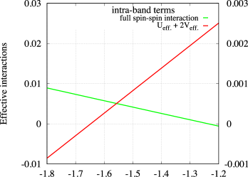
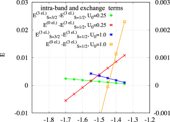
Figure 11: (a) Effective spin-spin interaction and $U_{eff.}+2V_{eff.}$ interaction from intra-band terms only for the system depicted in the figure 6 with the modified potentials and enlarged Kekule hoppings (see eq. 43) beyond the critical $\alpha=-1$ value. Left scale corresponds to charge-charge interaction, right scale corresponds to the spin-spin interaction. (b) Energy difference between $S=3/2$ and $S=1/2$ states with three electrons in the flat band; and energy difference between the state with empty flat band and the aforementioned $S=1/2$ state. Results obtained after exact diagonalization of the effective Hamiltonian 20 taking into account exchange terms. The system is the same as in the figure (a).

III.2 Frustrated spin-spin interaction beyond the edge of the parameters’ region accessible for QMC

Now we switch to $\alpha$ values outside of the limit accessible to QMC simulations. Results for the effective spin-spin interaction $J^{(\Sigma)}_{eff.}$ obtained from intra-band terms at $\alpha<-\sqrt{1/10}$ are shown in Fig. 10. As one can see, the spin-spin interaction becomes positive, thus the whole spin system in the flat band becomes frustrated. There is one peculiarity though. Large negative values of $\alpha$ lead to large negative effective charge-charge interaction, which is evident from Fig. 7. Eventually, it leads to the change of the ground state. If $\alpha$ is far enough from $-\sqrt{1/10}$, the ground state does not belong any more to the subspace with three electrons in the flat band. Instead, it belongs to the subspaces, where the number of electrons is either zero or six (empty or completely filled flat band). We already saw this effect in the fitting procedure for the QMC data 42, where we needed to take into account this state as a first excitation beyond the localized $S=3/2$ and $S=1/2$ states. The corresponding effective interaction $U_{eff.}+2V_{eff.}$ is shown in Fig. 10. If this interaction is negative, the ground state becomes charged and we loose localization. However, it happens after $J^{(\Sigma)}_{eff.}$ becomes positive, thus there is a narrow region of $\alpha$ values, where the electrons are still localized and simultaneously frustrated. In this case, the ground state has $S=1/2$ and is four-fold degenerate (two degenerate $S=1/2$ states with additional $M_{z}=\pm 1/2$ degeneracy).

The energy scale in Fig. 10 is quite small. We can change this scale by changing the interaction matrix $U$. Example calculations are shown in Fig. 11. The geometry of this system is the same as the one shown in Fig. 6, but the larger Kekule hoppings are now equal to 1.5. $U$ matrix for the interacting dimers also differs. It is now defined as

$$U=U_{0}\begin{pmatrix}1&\alpha\\ \alpha&1\end{pmatrix}$$ (43)

As one can see, the scale of the effective spin-spin interaction is now ten times larger and the frustrated ground state of localized spins exists in a much broader interval of $\alpha$ values.

Finally, we check that the effect survives the introduction of exchange terms in the effective Hamiltonian. The corresponding calculation is shown in Fig.11. Results are shown for $U_{0}=0.25$ and $U=1.0$, the values, where the results of the exact diagonalization of the approximate effective Hamiltonian were essentially indistinguishable from the exact ones obtained using QMC. We compute the energies of $S=1/2$ and $S=3/2$ states in the subspace with three electrons in the flat band (denoted as $E^{(3el.)}_{S=1/2}$ and $E^{(3el.)}_{S=2/2}$ in Fig. 11) and the energy of the empty flat band (denoted as $E^{(0el.)}$). $E^{(3el.)}_{S=3/2}>E^{(3el.)}_{S=1/2}$ for both $U_{0}=0.25$ and $U=1.0$ for all $\alpha$ values used in the computation. This means that effective spin-spin interaction within the flat band is still frustrating even after the inclusion of the exchange terms for $\alpha<\alpha_{1}$, where $\alpha_{1}$ is some critical value. In addition to that $E^{(0el.)}>E^{(3el.)}_{S=1/2}$ for $\alpha>\alpha_{0}$ with $\alpha_{0}$ dependent on $U_{0}$. Combining these two inequalities, we conclude that there is an interval $\alpha_{0}<\alpha<\alpha_{1}$, where the electrons in the flat band are localized and frustrated.

Even if there are some doubts about the approximations made during the derivation of the effective Hamiltonian 20, the limit $U_{0}/m\rightarrow 0$ stabilizes the frustrated state in any case. The reason is the diminishing role of the exchange terms in 20 in the limit of a large gap. It means that the intra-band results shown in the figure 11 eventually become exact, after appropriate rescaling due to decreasing $U_{0}$ and we still obtain frustrated localized spins within the flat band in a certain interval of $\alpha$ values.

Conclusion

We constructed a two-dimensional lattice model with a flat band generated by adatoms placed on top of a hexagonal lattice. An approximate effective Hamiltonian is constructed for the flat band assuming a large gap between conduction and valence bands. Our projection algorithm is verified using exact QMC data for the sign problem free system. Subsequently, this verified projection algorithm is used to construct a lattice model, featuring a trimer of localized electrons in a flat band, interacting via frustrating antiferromagnetic interaction. This lattice model is formulated on bipartite lattice and preserves particle-hole and SU(2) spin symmetry. However, in order to generate frustration in the effective Hamiltonian in the flat band, we need the combination of repulsive Hubbard interaction and large attractive long-range charge-charge interactions. This combination leads to the presence of both positive and negative eigenvalues in the charge-charge interaction matrix, thus making this model inaccessible to usual QMC simulations.

We hence provide an explicit mapping between two classes of quantum systems, both of them being problematic for QMC calculations in the sense that they generically lead to a negative sign problem. However, if algorithmic progress is achieved for systems with dominant long-range charge-charge interaction, our mapping will immediately provide a solution for the sign problem for frustrated spin systems.

As a final note, we would like to comment on the possibility to simulate systems where long-range interaction dominates over Hubbard interaction using the same trick with flat band projection. The question is if we can generate a sign problem free lattice model accessible to determinantal QMC, and featuring a flat band, where e.g. nearest-neighbour charge-charge interaction dominates over Hubbard repulsion. As shown in the Appendix A, the answer is negative. In order to make such simulations feasible, we again need to cross the point in the parameter space, where at least one eigenvalue of the interaction matrix 2 changes sign. Thus such simulations are again unfeasible with present-day QMC algorithms.

More generally, flat bands provide an extremely rich playground to investigate correlation induced phenomena, a modern example being twisted bilayer graphene Cao et al. (2018). While single electron hoping is suppressed interactions in the particle-hole channel, as described here, as well as in the particle-particle channel can be manipulated by tailoring the form of the Wannier functions of the flat band Peri et al. (2021); Hofmann et al. (2023). Frustrated spin systems, considered in the paper are not realistic due to the peculiar setup we used for the electron-electron interaction. However, the projection algorithm described in the paper can be used to model experimentally relevant systems, where frustration in the flat band, formed by adatoms can be achieved through different mechanisms. In particular if we relax the particle-hole symmetry condition in the free Hamiltonian, $\hat{H}_{K}$, then the Coulomb interaction can lead to frustrated effective spin-spin interaction in the flat band. This route to design frustrated spin systems is left for future research.

Appendix A Stability of zero eigenvalue of interaction matrix

In this appendix we study the possibility to create a flat band system with nearest-neighbour interaction larger than the Hubbard interaction. Minimal system, where this effect can be studied consists of two adatoms, creating two zero modes in non-interaction Hamiltonian, as depicted in the schemes A.A.1 and A.A.1. In the first scheme, matrix of interactions $U$ consists of only one dimer and is defined as

$$U=U_{0}\begin{pmatrix}1&\alpha\\ \alpha&1\end{pmatrix}.$$ (44)

This dimer connects two equivalent sites near the adatoms. Interaction matrix has zero mode if $\alpha=\pm 1$, and this zero mode is preserved in the effective interactions $V_{eff.}$ and $U_{eff.}$ computed from intra-band terms 26, 28. The latter is evident from the inset on the figure A.A.1, where $V_{eff.}=-U_{eff.}$ at $\alpha=-1.0$.

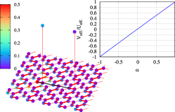
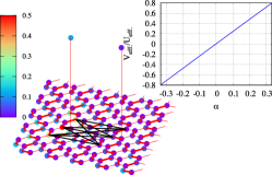
Figure A.1: Scheme of hoppings and interactions for system with two adatoms. Hoppings inside hexagonal lattice form Kekule pattern, bold lines correspond to $t=1.3$, thin lines correspond to $t=1.0$. Hopping to adatom is equal to $t^{\prime}=10.0$. Color scale corresponds to the modulus of the Wannier wavefunction, concentrated around one of the additional sites. Figure (a) displays the setup when charge-charge interaction consists of one dimer 44. Figure (b) shows the situation when matrix of potential includes more connections between sites, where Wannier wavefunctions for flat band states have the largest absolute values 45. Insets: $\alpha$-dependence of the ratio of effective nearest-neighbour interaction 28 to effective Hubbard interaction 26 if only intra-band terms are taken into account.

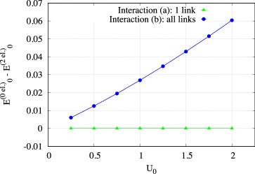
Figure A.2: Energy difference between the level, where the flat band is empty and the lowest level in the subspace with two electrons in the flat band. The latter level corresponds in both cases to the degenerate state of localized spins with $S=1$ and $S=0$. Calculations were done for negative limiting values of $\alpha$: $\alpha=-1.0$ in (a) case and $\alpha=-1/3$ in (b) case. Corresponding systems are shown in the figures A.A.1 and A.A.1.

In the second scheme, the interaction Hamiltonian $H_{U}$ includes three sites with the largest electronic density of the corresponding Wannier function near each adatom. If the first three charges correspond to the sites near one adatom, and the last three charges correspond to the sites near another adatom, the matrix of interactions looks like:

$$U=U_{0}\begin{pmatrix}1&0&0&\alpha&\alpha&\alpha\\ 0&1&0&\alpha&\alpha&\alpha\\ 0&0&1&\alpha&\alpha&\alpha\\ \alpha&\alpha&\alpha&1&0&0\\ \alpha&\alpha&\alpha&0&1&0\\ \alpha&\alpha&\alpha&0&0&1\end{pmatrix}.$$ (45)

As displayed in the figure A.A.1, the matrix of interactions includes all possible interactions between sites locates near different adatoms, but does not include non-local interactions between sites located near the same adatom. $U$ matrix 45 has zero eigenvalue if $\alpha=\pm 1/3$. However, the zero mode is not transferred to the effective interactions in this case: it is evident from the inset in the figure AA.1: $V_{eff.}\neq-U_{eff.}$ at $\alpha=-1/3$, though absolute value of $V_{eff.}$ grows linearly with increasing $|\alpha|$.

The following broad statement can be formulated: we can write down a general interaction matrix and try to optimize it within the constraint that it has no negative eigenvalues. Maximum what we can get from intra-band terms only is the situation when $|V_{eff.}|=U_{eff.}$, and it appears only when there is a zero mode in the interaction matrix $U$. The first system (fig. A.A.1) gives an example of such situation. In all other cases, the constraint leads to $|V_{eff.}|<U_{eff.}$ as it is for the second system (fig. A.A.1). It also shows that the presence of the zero mode in $U$ matrix does not always lead to $|V_{eff.}|=U_{eff.}$.

The only remaining possibility is that the exchange terms can drive the effective potentials through this border ($|V_{eff.}|=U_{eff.}$). In order to explore it, we diagonalize the full effective Hamiltonian 20 and compare the energy of the state with empty flat band and the energy of the lowest state with two electrons in the flat band. Results for both systems are shown in the figure A.2. We always choose the smallest negative $\alpha$ possible within the constraint of non-negative eigenvalues of the interaction matrix $U$.

For the first system, the two states in question remain degenerate independently from the interaction strength $U_{0}$. It means that $V_{eff.}=-U_{eff.}$ even after the inclusion of the exchange terms. Thus, the initial zero mode is stable not only with respect to the intra-band terms, but also with respect to the exchange terms.

For the second system, the energy difference is dependent on the interaction strength $U_{0}$, but it unfortunately evolves in the opposite direction to the desired one. Increasing $|V_{eff.}|$ with $V_{eff.}<0$ should lead to decreasing difference $E^{0el.}_{0}-E^{2el.}_{0}$ so that the state with empty flat band becomes the ground state. The plot shows exactly opposite evolution.

Thus we can conclude that there is no possibility to have $|V_{eff.}|>U_{eff.}$ within the constraint of non-negative eigenvalues of the interaction matrix $U$. There are only two scenarios: 1) $|V_{eff.}|=U_{eff.}$ in intra-band Hamiltonian (can only happen when $U$ has zero mode), but this situation remains unchanged after the inclusion of the exchange terms; 2) $|V_{eff.}|<U_{eff.}$ in intra-band Hamiltonian, but the exchange terms only reduce the $|V_{eff.}|/U_{eff.}$ ratio.