Flavor asymmetry of light sea quarks in proton : A light-front spectator model

Abstract

We formulate a light-front spectator model for the proton that incorporates the presence of light sea quarks. In this particular model, the sea quarks are seen as active partons, whereas the remaining components of the proton are treated as spectators. The proposed model relies on the formulation of the light-front wave function constructed by the soft wall AdS/QCD. The model wave functions are parameterized by fitting the unpolarized parton distribution functions of light sea quarks from the CTEQ18 global analysis. We then employ the light-front wave functions to obtain the sea quarks generalized parton distribution functions, transverse momentum dependent parton distributions, and their asymmetries, which are accessible in the upcoming Electron-Ion-Colliders. We investigate sea quarks’ spin and orbital angular momentum contributions to the proton spin.

I Introduction

Quantum chromodynamics (QCD) is the well-established theory for the strong interactions, where the proton is viewed as a strongly coupled and correlated confined system of quarks and gluons. The original quark model, where the proton is described by two up quarks ($u$) and one down quark ($d$), has an appealing simplicity. However, various experiments that measure the parton distribution functions (PDFs) have revealed a substantial structure with additional quarks, antiquarks, and gluons beyond the leading three-quark Fock component. These additional quarks and antiquarks are known as sea quarks. It is not possible to distinguish any individual down or up quark as a valence or sea quark, but antiquarks must belong to the sea and so their study promises to illuminate new insights into the structure of the proton. Going beyond the leading Fock component $|uud\rangle$, the concept of the five-particle Fock state with charm sea quark, $|uudc\bar{c}\rangle$, in the proton was first suggested by Brodsky et. al. Brodsky et al. (1980, 1981). The sea-quark distributions in the proton, together with the valence quark and gluon distributions, have been investigated in numerous experiments employing the deep inelastic scattering (DIS), the Drell-Yan, and other hard processes Drell and Yan (1971); Chang and Peng (2014). In the study of sea quarks in the proton, several asymmetries such as $\bar{d}-\bar{u}$, $\bar{d}/\bar{u}$ and $(\bar{d}-\bar{u})/(\bar{u}+\bar{d})$ originating from the flavor asymmetry have been observed Buccella and Soffer (1993); Kumano (1998). It states that the anti-up quark and the anti-down quark distributions are not the same within the proton. The initial naive expectation was that the sea quark distributions of up and down quark are the same as the sea was generated predominantly by gluons splitting into quark-antiquark pairs and the splitting is flavor independent and the masses of up and down quarks are also almost degenerate. However, the deviation of this assumption can be evaluated by the following expression

$$S_{G} = \int_{0}^{1}\left[F_{2}^{p}(x)-F_{2}^{n}(x)\right]\frac{{\rm d}x}{x}=\frac{1}{3}\int_{0}^{1}\left[u_{v}(x)-d_{v}(x)\right]{\rm d}x-\frac{2}{3}\int_{0}^{1}\left[\bar{d}_{p}(x)-\bar{u}_{p}(x)\right]{\text{d}x}\,$$ (1)

$$= \frac{1}{3}-\frac{2}{3}\int_{0}^{1}\left[\bar{d}_{p}(x)-\bar{u}_{p}(x)\right]{\text{d}x}\,,$$

where $F_{2}^{p}(x)$ and $F_{2}^{n}(x)$ are the proton and the neutron inelastic structure functions, respectively; $u_{v}(x)$ and $d_{v}(x)$ are the valence quark distributions in the proton; and $\bar{d}_{p}(x)$ and $\bar{u}_{p}(x)$ are the anti-down and the anti-up quark distributions in the proton sea as a function of Bjorken-$x$. Equation (1) requires the assumption of charge symmetry between the proton and the neutron (i.e. $u_{p}=d_{n}$, $\bar{u}_{p}=\bar{d}_{n}$, etc.,). If the nucleon sea is flavor symmetric in light quarks, then the value of $S_{G}=1/3$, a result referred as the Gottfried Sum Rule (GSR) Gottfried (1967). In the early 1990’s, the New Muon Collaboration (NMC) Amaudruz et al. (1991); Arneodo et al. (1994) announced a precise DIS measurement indicating a violation of the GSR Gottfried (1967), which leads to an asymmetries between the $\bar{u}$ and $\bar{d}$ distributions in the proton. The NMC Collaboration reported a value of $S_{G}=0.235\pm 0.026$ Kumano (1991), which implies that

$$\int_{0}^{1}\left[\bar{d}_{p}(x)-\bar{u}_{p}(x)\right]{\rm d}x=0.147\pm 0.039,$$ (2)

a considerable excess of $\bar{d}$ relative to $\bar{u}$ in the proton.

The discovery of the flavor asymmetry in the nucleon sea triggered numerous dedicated experimental and theoretical efforts Chang and Peng (2014); Buccella and Soffer (1993); Kumano (1998); Wakamatsu (2014); Lin et al. (2015); Song et al. (2011); Brodsky et al. (2022); Garvey and Peng (2001); Dove et al. (2023); Accardi et al. (2020); Kotlorz et al. (2021); Hawker et al. (1998); Peng et al. (1998); Dove (2020); Nagai (2019); McGaughey et al. (1992); Choudhary et al. (2023); Dorokhov and Kochelev (1991, 1993); Trevisan et al. (2008); He et al. (2022). The study of sea quarks’ properties within the nucleon becomes one of the major goals at the Large Hadron Collider (LHC) Rojo et al. (2015); Harland-Lang et al. (2015) and the future Electron-Ion-Colliders (EICs) Accardi et al. (2016); Abdul Khalek et al. (2022); Anderle et al. (2021). The sea quark asymmetry is not only observed in the light flavors but also in the strange Cao (2016); He and Wang (2018) and the heavy flavors Brodsky et al. (2022); Lyubovitskij and Schmidt (2023); Sufian et al. (2020). In this work, we focus on the light sea quarks. The light flavor asymmetries have been measured experimentally by several collaborations Dove et al. (2023); Accardi et al. (2020); Kotlorz et al. (2021); Hawker et al. (1998); Peng et al. (1998); Dove (2020); Nagai (2019); McGaughey et al. (1992); Towell et al. (2001); Dove et al. (2021); Ackerstaff et al. (1998). The results from the NuSea/E866 Collaboration Towell et al. (2001) demonstrate a rapid growth of $\bar{d}(x)/\bar{u}(x)$ up to $x\lesssim 0.2$ and then a sharp fall of this ratio in the region $x>0.2$. However, the recent measurement by the SeaQuest/E906 Collaboration Dove et al. (2021, 2023) shows a modest growth of $\bar{d}(x)/\bar{u}(x)$ at the region $0.13<x<0.45$. The trends between these two experiments at higher $x$ region are quite different. No explanation has been found yet for the differing results. The experimental data is not available for the entire $x$ region. The data of $\bar{d}(x)-\bar{u}(x)$ from the HERMES Collaboration are more or less consistent with the prominent features as shown by the NuSea/E866 Towell et al. (2001) and the SeaQuest/E906 Dove et al. (2021, 2023) Collaboration, where the asymmetry is expected to fall monotonously as $x$ increases. A precise knowledge of the sea quark distributions is required for the analysis and interpretation of the scattering experiments in the LHC era. Global fitting collaborations such as CTEQ Dulat et al. (2016), NNPDF Ball et al. (2017), HERAPDF Alekhin et al. (2017), MSTW Martin et al. (2009), and MMHT Harland-Lang et al. (2015) have made considerable efforts to determine sea quark PDFs and their uncertainties. The proton sea has also been investigated using different theoretical approaches such as the chiral quark model Song et al. (2011); Choudhary et al. (2023), instanton model Dorokhov and Kochelev (1991, 1993), statistical model Trevisan et al. (2008), chiral soliton model Thomas (1983), chiral light-front perturbation theory Alberg and Miller (2019), chiral effective theory Wang et al. (2023), lattice QCD Lin et al. (2015); Alexandrou et al. (2021), BHPS model Chang and Peng (2011), etc. In Ref. Henley and Miller (1990) the asymmetry is explained in terms of pion cloud effects and by imposing constraints on the pion-nucleon vertex function. A common feature of most of these theoretical approaches is a growth of $\bar{d}(x)/\bar{u}(x)$ with increasing $x$, consistent with the characteristic shown by the NuSea/E866 data at lower-$x$ and the SeaQuest/E906 data. An overview of the nucleon sea and their asymmetries can be found in Refs.  Kumano (1998); Geesaman and Reimer (2019); Chang and Peng (2014). The spin structure of sea quarks is an additional captivating element to consider. The sea quark helicity distributions Geesaman and Reimer (2019); Chang and Peng (2014) could give us important clues about how to solve the nucleon spin puzzle Ji et al. (2021).

Recently, there are numerous experiments and theoretical investigations Chekanov et al. (2003); Alekseev et al. (2009); Airapetian et al. (2009) aimed to understand the generalized parton distributions (GPDs) and the transverse momentum parton dependent distributions (TMD), which encode the three-dimensional (3D) information of the quark in the proton. The GPDs Diehl (2003); Belitsky and Radyushkin (2005); Goeke et al. (2001); Ji (1998); Burkardt (2003) are required for exclusive processes such as deeply virtual Compton scattering (DVCS) Ji (1997a); Goeke et al. (2001) or vector meson productions Goloskokov and Kroll (2008); Collins et al. (1997), while the TMDs Collins et al. (1985); Boer and Mulders (1998); Angeles-Martinez et al. (2015) are necessary to explain the Semi-Inclusive Deep Inelastic Scattering (SIDIS) Bacchetta et al. (2007); Ji et al. (2005) or Drell-Yan processes Tangerman and Mulders (1995); Collins (2002); Zhou et al. (2010). The GPDs give us with valuable information about the spatial distributions, spin and orbital motion of quarks inside the proton. The TMDs, on the other hand, are the extended version of collinear PDFs, capturing the 3D structural information of the proton in momentum space. The TMDs also encode the knowledge about the correlations between spins of the proton and momenta of the quarks. While the valence quark GPDs and TMDs have been investigated for decades and are determined from various theoretical approaches Alexandrou et al. (2020); Lin (2022); Ji et al. (1997); Scopetta and Vento (2003); Petrov et al. (1998); Penttinen et al. (2000); Boffi et al. (2003, 2004); Vega et al. (2011); Chakrabarti and Mondal (2013a); Mondal and Chakrabarti (2015); Chakrabarti and Mondal (2013b); Mondal (2017); de Teramond et al. (2018); Xu et al. (2021); Liu et al. (2022); Kaur et al. (2023); Avakian et al. (2010); Efremov et al. (2009); Bastami et al. (2021); Bacchetta et al. (2008); Maji and Chakrabarti (2017); Pasquini et al. (2008); Musch et al. (2011); Ji et al. (2015); Hu et al. (2022), much less information is available on the sea quark distributions. Recently, the sea quark GPDs in the proton have been investigated with the nonlocal covariant chiral effective theory He et al. (2022) and using a light-cone baryon-meson fluctuation model Luan and Lu (2023). To our knowledge, the study of sea quark TMDs in the proton not yet available in the literature. Precise determination of 3D structure of the proton, specifically the sea quark and gluon distributions, are two of the major scientific objectives of the upcoming EICs Accardi et al. (2016); Abdul Khalek et al. (2022); Anderle et al. (2021).

In this work, we construct a light-front spectator model for the proton embodying the light sea quarks, which are seen as active partons and the remaining components of the proton are considered as spectators. We model the light-front wave functions using the wave functions predicted by the soft-wall AdS/QCD and parameterize them by fitting the unpolarized PDFs of light sea quarks from the CTEQ global analysis at the scale $Q=2$ GeV Hou et al. (2021). We then investigate the asymmetries of sea quarks in this model by employing the resulting light-front wave functions. We compare our model predictions for the $\bar{d}(x)-\bar{u}(x)$ and $\bar{d}(x)/\bar{u}(x)$ with the available experimental data from the NuSea/E866 Towell et al. (2001), HERMES Ackerstaff et al. (1998), and SeaQuest/E906 Dove et al. (2023) Collaborations as well as with the CTEQ18 global fit Hou et al. (2021). We further study the sea quarks asymmetries through their GPDs and TMDs in this model and also investigate sea quarks spin and orbital angular momentum (OAM) contributions to the proton spin.

The paper is organized as follows: In section II, we discuss about our model construction and determine the value of model parameters by fitting the unpolarized sea quark PDFs to the CT18NNLO global analyses Hou et al. (2021). We present the comparison between our model predictions for the flavor asymmetries and the experimental data in this section. The sea quark helicity and transversity PDFs are also presented in this section. We evaluate the sea quark GPDs and the OAM in section III. Flavor asymmetries for sea quarks at finite momentum transfer are obtained from the calculated GPDs and the results are discussed in this section. Section IV presents the sea quark TMDs and describes the flavor asymmetries for sea quarks in the transverse momentum plane. We discuss a different phenomenological model and reevaluate all the sea quark distributions and compare them with the previous results in section V. We provide a summary in section VI.

II Model description

QCD predicts the existence of both perturbative extrinsic and nonperturbative intrinsic quark contributions to the structure of hadrons. We analyze the sea quark content in the proton, induced either directly by the nonperturbative $|qqqq\bar{q}\rangle$ Fock component or by the $|qqqg\rangle$ Fock component, where the gluon splits into a quark-antiquark pair. The complete distribution of sharing the longitudinal momentum could be written as sum of the intrinsic and the extrinsic distributions. The intrinsic quarks are observed in the low energy region, while the extrinsic sea quarks resulting from gluon splitting appear in relatively high energy.

The light-front formalism provides a convenient way to study the hadronic system. Here we adopt the generic ansatz for the light-front quark-spectator model for the proton Brodsky et al. (2022). In this model, one contemplates the proton as an effective system composed of an active sea quark (fermion) and a composite state of spectator (boson), where the spin of the spectator is assumed to be zero (scalar) only. We model the light-front wave functions from the solution of soft-wall AdS/QCD. The $2$-particle Fock-state expansion for proton with spin components: $J^{z}=\pm 1/2$, in a frame, where the transverse momentum of proton vanishes, i.e., $P\equiv\big{(}P^{+},\textbf{0}_{\perp},{M^{2}}/{P^{+}}\big{)}$, can be expressed as

$$|P;\uparrow(\downarrow)\rangle =\sum_{\bar{q}}\int\frac{{\rm d}x\,{\rm d}^{2}\textbf{k}_{\perp}}{2(2\pi)^{3}\sqrt{x(1-x)}}\Big{[}\psi^{\uparrow(\downarrow)}_{\bar{q};+\frac{1}{2}}(x,\textbf{k}_{\perp})|+\frac{1}{2},0;xP^{+},\textbf{k}_{\perp}\rangle+\psi^{\uparrow(\downarrow)}_{\bar{q};-\frac{1}{2}}(x,\textbf{k}_{\perp})|-\frac{1}{2},0;xP^{+},\textbf{k}_{\perp}\rangle\Big{]}.$$ (3)

For nonzero transverse momentum of the proton, i.e., ${\bf P}_{\perp}\neq 0$, the physical transverse momenta of the active quark and the spectator are ${\bf p}_{\perp}^{\bar{q}}=x{\bf P}_{\perp}+{\bf k}_{\perp}$ and ${\bf p}_{\perp}^{S}=(1-x){\bf P}_{\perp}-{\bf k}_{\perp}$, respectively, where ${\bf k}_{\perp}$ corresponds to the relative transverse momentum of the constituents. $\psi_{\bar{q};\lambda_{\bar{q}}}^{\lambda_{p}}(x,{\bf k}_{\perp})$ represent the light-front wave functions with helicities of the proton $\lambda_{p}=\uparrow(\downarrow)$ and the sea quark $\lambda_{\bar{q}}=\pm\frac{1}{2}$. The light-front wave functions at an initial scale $Q_{0}=2$ GeV are given by

$$\psi^{\uparrow}_{\bar{q};+\frac{1}{2}}(x,{\bf k}_{\perp}) = \varphi(x,{\bf k}_{\perp}^{2})$$

$$\psi^{\uparrow}_{\bar{q};-\frac{1}{2}}(x,{\bf k}_{\perp}) = -\dfrac{k^{1}+ik^{2}}{\kappa}\,\varphi(x,{\bf k}_{\perp}^{2})\,,$$

$$\psi^{\downarrow}_{\bar{q};+\frac{1}{2}}(x,{\bf k}_{\perp}) = -\Big{[}\psi^{\uparrow}_{\bar{q};-\frac{1}{2}}(x,{\bf k}_{\perp})\Big{]}^{\dagger}=\dfrac{k^{1}-ik^{2}}{\kappa}\,\varphi(x,{\bf k}_{\perp}^{2})\,,$$

$$\psi^{\downarrow}_{\bar{q};-\frac{1}{2}}(x,{\bf k}_{\perp}) = \Big{[}\psi^{\uparrow}_{\bar{q};+\frac{1}{2}}(x,{\bf k}_{\perp})\Big{]}^{\dagger}=\varphi(x,{\bf k}_{\perp}^{2})\,,$$ (4)

where $\varphi(x,{\bf k}_{\perp}^{2})$ is the modified soft wall AdS/QCD wave function Chakrabarti et al. (2023),

$$\varphi(x,{\bf k}_{\perp})=\sqrt{A}\frac{4\pi}{\kappa}\sqrt{\frac{\log[1/(1-x)]}{x}}x^{\alpha}(1-x)^{3+\beta}\exp{\left[-\frac{\log[1/(1-x)]}{2\kappa^{2}x(1-x)}{\bf k}_{\perp}^{2}\right]},$$ (5)

with $\alpha$ and $\beta$ are our model parameters. We consider the AdS/QCD scale parameter $\kappa=0.4$ GeV Chakrabarti and Mondal (2013a). The values of the model parameters $\alpha$ and $\beta$, and the normalization constant $A$ are fixed by fitting the light sea quarks unpolarized PDFs at the scale $Q_{0}=2$ GeV with CTEQ18 next-to-next-leading order (NNLO) data.

The PDF, the probability that a parton carries a certain fraction of the total light-front longitudinal momentum of the proton, provides us information about the nonperturbative structure of the proton. The sea quark PDF of the proton, which encodes the distribution of longitudinal momentum and polarization carried by the sea quark in the proton, can be expressed in terms of the light-front wave functions. The unpolarized sea quark PDF at the model scale reads

$$f_{1}(x) = \int\frac{{\rm d}^{2}{\bf k}_{\perp}}{16\pi^{3}}\,\left[|\psi^{\uparrow}_{\bar{q};+\frac{1}{2}}(x,{\bf k}_{\perp})|^{2}+|\psi^{\uparrow}_{\bar{q};-\frac{1}{2}}(x,{\bf k}_{\perp})|^{2}\right]$$

$$= \int\frac{{\rm d}^{2}{\bf k}_{\perp}}{16\pi^{3}}\,\left[|\psi^{\downarrow}_{\bar{q};+\frac{1}{2}}(x,{\bf k}_{\perp})|^{2}+|\psi^{\downarrow}_{\bar{q};-\frac{1}{2}}(x,{\bf k}_{\perp})|^{2}\right]\,$$

$$= Ax^{2\alpha}(1-x)^{7+2\beta}\left(1+\frac{x(1-x)}{\log\frac{1}{1-x}}\right)\,,$$

while the helicity PDF is expressed as

$$g_{1L}(x) = \int\frac{{\rm d}^{2}{\bf k}_{\perp}}{16\pi^{3}}\,\left[|\psi^{\uparrow}_{\bar{q};+\frac{1}{2}}(x,{\bf k}_{\perp})|^{2}-|\psi^{\uparrow}_{\bar{q};-\frac{1}{2}}(x,{\bf k}_{\perp})|^{2}\right]$$

$$= \int\frac{{\rm d}^{2}{\bf k}_{\perp}}{16\pi^{3}}\,\left[|\psi^{\downarrow}_{\bar{q};+\frac{1}{2}}(x,{\bf k}_{\perp})|^{2}-|\psi^{\downarrow}_{\bar{q};-\frac{1}{2}}(x,{\bf k}_{\perp})|^{2}\right]\,$$

$$= Ax^{2\alpha}(1-x)^{7+2\beta}\left(1-\frac{x(1-x)}{\log\frac{1}{1-x}}\right)\,,$$

and the Transversity PDF is given by

$$h_{1}(x) = \int\frac{{\rm d}^{2}{\bf k}_{\perp}}{16\pi^{3}}\psi^{\uparrow\dagger}_{\bar{q};+\frac{1}{2}}(x,\textbf{k}_{\perp})\psi^{\downarrow}_{\bar{q};-\frac{1}{2}}(x,\textbf{k}_{\perp})\,,$$ (8)

$$= Ax^{2\alpha}(1-x)^{7+2\beta}\,.$$

Table 1: Fitted model parameters at $Q_{0}=2$ GeV.

	A	$\alpha$	$\beta$
$\overline{u}$	$0.055_{-0.002}^{0.003}$	$-0.611_{0.001}^{0.001}$	$-1.33_{-0.181}^{-0.131}$
$\overline{d}$	$0.082_{0.007}^{-0.006}$	$-0.572_{0.016}^{-0.014}$	$-1.33_{0.163}^{-0.132}$

II.1 Numerical fitting and model parameters

There are three parameters $\alpha$, $\beta$, and $A$ in our model that manifest the goodness of the model. The parameter $A$ is a free parameter, which decides the amplitude of the sea quark PDF in the $x$ close to zero region. The parameters $\alpha$ and $\beta$ decide the behavior of the distributions in extreme limits of $x$. The parameter $\alpha$ is crucial to lower $x$, while $\beta$ controls large $x$ behaviour of the distributions. We determine these parameters by fitting the model unpolarized light sea quark distributions with the latest available data at NNLO of the sea quark distributions $x{\bar{u}}(x)$ and $x{\bar{d}}(x)$ from the global analysis by the CTEQ Collaboration Hou et al. (2021). We particularly fit CTEQ18 NNLO sea quark PDFs at the scale $Q_{0}=2$ GeV. We choose 201 number of data points distributed logarithmically within the interval $0.001<x<1$. There are $58$ CTEQ18 NNLO replicas accessible along the centre line. The zeroth replicas represent the central lines of the distributions. We determine the central values of our model parameters by fitting those zeroth replicas of the CTEQ18 NNLO data. We choose replicas number $4$ and $8$ for the $\bar{d}$ and the $\bar{u}$ PDFs, respectively from the data to estimate the uncertainties in our model parameters. The value of $\chi^{2}$ per degree of freedom (d.o.f.) for the fit of the $x{\bar{d}}(x)$ is $0.271$, whereas for the $x{\bar{u}}(x)$ the value of $\chi^{2}$/d.o.f. is $0.0409$ in the region $0.001<x<0.1$. The value of $\chi^{2}$ enlarges in the high $x$ region particularly for the $\bar{u}$ sea quarks. The fitted model parameters with their uncertainties are listed in Table 1.

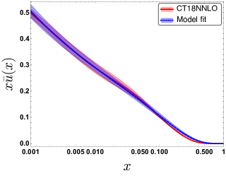
Figure 1: Sea quark unpolarized distributions in the proton, left panel: $x{\bar{d}}(x)$ and right panel: $x{\bar{u}}(x)$ as a function of longitudinal momentum fraction $x$ in the kinematics region $0.001\leq x\leq 1$ at $Q_{0}=2$ GeV. Our model results (dashed-blue lines with blue bands) are compared with the CTEQ18 NNLO dataset (solid-red lines with red bands) Hou et al. (2021)

.

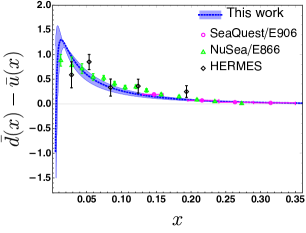
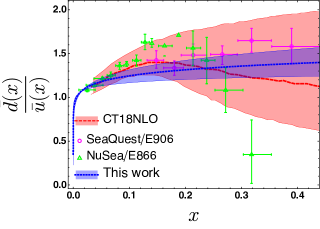
Figure 2: The light flavor sea asymmetries in the proton, left panel: $\bar{d}(x)-\bar{u}(x)$ and right panel: $\bar{d}(x)/\bar{u}(x)$ as a function of $x$. Our model results (blue dotted lines with blue bands) are compared with the experimental data from the SeaQuest/E906 Dove et al. (2023) (magenta open circle), NuSea/E866 Towell et al. (2001) (green open triangle), and HERMES Ackerstaff et al. (1998)(black open rombos) Collaborations. In the right panel, we also include the CTEQ18 NLO global analysis Hou et al. (2021) (red dashed lines with red bands) for the comparison.

Table 2: Value of $\int{\rm d}x\left[\bar{d}(x)-\bar{u}(x)\right]$ in different range of $x$. Our results are compared with various experiments.

Model/Experiments	$x$-range	$\int{\rm d}x\left[\bar{d}(x)-\bar{u}(x)\right]$
This work	$0.13<x<0.45$	$0.015\pm 0.004$
SeaQuest/E906 Dove et al. (2023)	$0.13<x<0.45$	$0.015\pm 0.003$
This work	$0.015<x<0.35$	$0.069\pm 0.015$
NuSea/E866 Towell et al. (2001)	$0.015<x<0.35$	$0.0803\pm 0.011$
NMC Arneodo et al. (1994)	$0.004<x<0.80$	$0.148\pm 0.039$
HERMES Ackerstaff et al. (1998)	$0.020<x<0.30$	$0.16\pm 0.03$

In Fig. 1, we show the results of our fits for the sea quark distributions, $x{\bar{u}}(x)$ and $x{\bar{d}}(x)$, at the scale $Q_{0}=2$ GeV. The solid red lines with the red bands identify the CTEQ analyses of those distributions Hou et al. (2021) and the dashed blue lines with the blue bands represent our results computed with the effective parameters. The second moments of the sea quark PDFs, which describe the average longitudinal momenta carried by the sea quarks are given by

$$\langle x\rangle_{\bar{d}} =\int_{0.001}^{1}{\rm d}x\,x{\bar{d}}(x)=0.039\pm 0.002\,,$$ (9)

$$\langle x\rangle_{\bar{u}} =\int_{0.001}^{1}{\rm d}x\,x{\bar{u}}(x)=0.032\pm 0.003\,.$$

We present the flavor asymmetries, ${\bar{d}}(x)-{\bar{u}}(x)$ and ${\bar{d}}(x)/{\bar{u}}(x)$, computed using our model wave functions in Fig. 2. We compare our prediction for ${\bar{d}}(x)-{\bar{u}}(x)$ with the available data from the SeaQuest/E906 Dove et al. (2023), HERMES Ackerstaff et al. (1998) and NuSea/E866 Towell et al. (2001) Collaborations in Fig. 2 (left plot). We find that below $x<0.01$, ${\bar{u}}(x)$ is larger than ${\bar{d}}(x)$ in our model and the $\bar{d}(x)-\bar{u}(x)$ asymmetry is opposite to what generally observed in the literature. However, this pattern has also been observed in the global analyses made by CT14 Dulat et al. (2016) and the latest NNPDF4.0 Ball et al. (2022) Collaborations. On the other hand, in the region $x>0.01$, we find more or less consistency between our result and the available experimental data Towell et al. (2001); Ackerstaff et al. (1998); Dove et al. (2023). Note that the value of the quantity $\int_{0}^{1}\left[\bar{d}(x)-\bar{u}(x)\right]dx$ depends on the energy scale of the measurement. The numerical results for the quantity at the scale $Q_{0}=2$ GeV for selected $x$ domains are given in Table 2. We compare our results with results from various experiments Arneodo et al. (1994); Ackerstaff et al. (1998); Towell et al. (2001). We find that our predictions are in good agreement with the SeaQuest/E906 results Dove et al. (2023) as shown in Table 2. Additionally, the SeaQuest/E906 Dove et al. (2023) result for the difference of second moments: $\int_{0.13}^{0.45}x\left[\bar{d}(x)-\bar{u}(x)\right]dx=0.00318^{+0.0005}_{-0.0006}$ is in excellent agreement with our model prediction: $\int_{0.13}^{0.45}x\left[\bar{d}(x)-\bar{u}(x)\right]dx=0.003\pm 0.001$.

Figure 2 (right plot) compares our result for the ${{\bar{d}}(x)}/{{\bar{u}}(x)}$ with the experimental data from the NuSea/E866 Towell et al. (2001), SeaQuest/E906 Dove et al. (2023) Collaborations as well as with the CTEQ18 NLO global analysis Hou et al. (2021). It can be noticed that there is a difference in qualitative behaviour between the SeaQuest/E906 data, which exhibits more or less flat behavior of the $\bar{d}(x)/\bar{u}(x)$ asymmetry, and the NuSea/E866 measurement showing a rapid fall of the ${{\bar{d}}(x)}/{{\bar{u}}(x)}$ in the region $x>0.2$. The trends between the two experiments at higher $x$ domain are quite different. As can be seen, our prediction for this asymmetry agrees well with the global fit and the trend of the latest experimental data from the SeaQuest/E906 Collaboration Dove et al. (2023) available in the range $0.015<x<0.35$. Meanwhile, Our result deviates from the overall behavior of portrayed by NuSea/E866 data Towell et al. (2001). In a Drell-Yan measurement at CERN, the NA51 Collaboration  Baldit et al. (1994) confirmed that $\bar{d}(x)$ is larger than $\bar{u}(x)$ at an average $x$ value of $0.18$. They reported $\bar{d}(x)/\bar{u}(x)|_{x=0.18}=1.96\pm 0.15\pm 0.19$, while in our model, we obtain $\bar{d}(x)/\bar{u}(x)|_{x=0.18}=1.30\pm 0.08$.

We show the results for helicity distribution for $\bar{d}$ and $\bar{u}$ in Fig. 3, where we compare our model predictions with the experimental data from the COMPASS Alekseev et al. (2010) and HERMES Airapetian et al. (2004) Collaborations. We find acceptable agreement between our sea quark helicity distributions and the experimental data. Note that the signs of sea quark helicity PDFs are not fixed by the experiments. The spin contribution of the $\bar{d}$ and $\bar{u}$ to the total proton spin can be quantified as the first moment of the helicity PDFs,

$$\Delta\Sigma^{\bar{d}} =\int_{0.001}^{1}{\text{d}x}g_{1L}^{\bar{d}}(x)=0.031\pm 0.001\,,$$ (10)

$$\Delta\Sigma^{\bar{u}} =\int_{0.001}^{1}{\text{d}x}g_{1L}^{\bar{u}}(x)=0.026\pm 0.002\,.$$

The sea quark’s transversity PDFs at the scale $Q_{0}=2$ GeV are shown in Fig. 4. They appear similar to unpolarized PDFs, mainly distributed at small-$x$ region and vanish after $x>0.5$. At small-$x$ ($<0.05$), $h_{1}^{\bar{u}}(x)$ dominates over $h_{1}^{\bar{d}}(x)$, whereas $h_{1}^{\bar{d}}(x)$ is larger than $h_{1}^{\bar{u}}(x)$ at $x>0.05$. The first moment of the transversity PDFs give the tensor charges. We find the sea quark tensor charges at the scale $Q_{0}=2$ GeV as

$$\delta{\bar{d}} =\int_{0.001}^{1}{\text{d}x}h_{1}^{\bar{d}}(x)=0.75\pm 0.05\,,$$ (11)

$$\delta{\bar{u}} =\int_{0.001}^{1}{\text{d}x}h_{1}^{\bar{u}}(x)=0.73\pm 0.04\,.$$

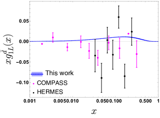
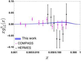
Figure 3: The helicity PDFs for $\bar{d}$ (left panel) and $\bar{u}$ (right panel) in the proton. Our model results (blue lines with blue bands) are compared with the experimental data from the COMPASS Alekseev et al. (2010) (magenta solid circle) and HERMES Airapetian et al. (2004) (black solid circle) Collaborations.

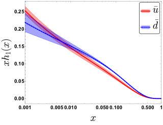
Figure 4: The transversity PDFs for $\bar{d}$ (blue line with blue band) and $\bar{u}$ (red line with red band) in the proton evaluated in our model.

III Sea quark GPDs

In general, the GPDs are obtained through the off-forward matrix elements of the bilocal operators between hadronic states. There are four chiral-even quark GPDs at leading twist, denoted as $H^{q}$, $E^{q}$, $\widetilde{H}^{q}$, and $\widetilde{E}^{q}$. The unpolarized ($H$ and $E$) and helicity-dependent ($\widetilde{H}$ and $\widetilde{E}$) quark GPDs for the nucleon are parameterized as Diehl (2001, 2003),

$$\frac{1}{2}\int\frac{\text{d}z^{-}}{2\pi}e^{i\bar{x}P^{+}z^{-}}\langle p^{\prime},\lambda^{\prime}|\bar{\psi}_{q}(-{z}/2)\gamma^{+}\psi_{q}({z}/2)|p,\lambda\rangle_{|_{z^{+}=0,\vec{z}_{\perp}=0}}=\frac{1}{2P^{+}}\bar{u}(p^{\prime},\lambda^{\prime})\bigg{[}H^{q}\gamma^{+}+E^{q}\frac{i}{2m}\sigma^{+\alpha}\Delta_{\alpha}\bigg{]}u(p,\lambda)\,,$$ (12)

$$\frac{1}{2}\int\frac{\text{d}z^{-}}{2\pi}e^{i\bar{x}P^{+}z^{-}}\langle p^{\prime},\lambda^{\prime}|\bar{\psi}_{q}(-{z}/2)\gamma^{+}\gamma_{5}\psi_{q}({z}/2)|p,\lambda\rangle_{|_{z^{+}=0,\vec{z}_{\perp}=0}}=\frac{1}{2P^{+}}\bar{u}(p^{\prime},\lambda^{\prime})\left[\widetilde{H}^{q}\,\gamma^{+}\gamma_{5}+\widetilde{E}^{q}\,\frac{\gamma_{5}\Delta^{+}}{2m}\right]u(p,\lambda)\,,$$ (13)

where $\psi_{q}(x)$ represents the quark field in the light-cone gauge. The momenta of the nucleon initial and final states are denoted by $p$ and $p^{\prime}$, respectively, with their corresponding helicities denoted as $\lambda$ and $\lambda^{\prime}$ and $m$ is the nucleon mass. The light-front spinor for the nucleon is denoted by $u(p,\lambda)$. The momentum transfer in this picture is expressed as $\Delta^{\mu}=p^{\prime\mu}-p^{\mu}$, while the skewness is given by $\zeta=-\frac{\Delta^{+}}{2\bar{P}^{+}}$. In this work, we consider the zero skewness case ($\zeta=0$) and thus only study the kinematic region corresponding to $\zeta<x<1$ also called the DGLAP region. The invariant momentum transfer in the process is denoted by $t=\Delta^{2}$ and for zero skewness, one has $t=-\Delta_{\perp}^{2}$. Note that one has to take into account nonzero skewness to compute $\widetilde{E}^{g}$. The remaining three chiral-even quark GPDs at leading twist can be written in terms of diagonal overlap of LFWFs as follows:

$$H^{\bar{q}}(x,0,-\Delta_{\perp}^{2}) =\int\frac{\text{d}^{2}{\bf k}_{\perp}}{16\pi^{3}}\,\biggl{[}\psi^{\dagger\uparrow}_{\bar{q};+\frac{1}{2}}(x,{\bf k}_{\perp}^{\prime\prime})\,\psi^{\uparrow}_{\bar{q};+\frac{1}{2}}(x,{\bf k}_{\perp}^{\prime})+\psi^{\dagger\uparrow}_{\bar{q};-\frac{1}{2}}(x,{\bf k}_{\perp}^{\prime\prime})\,\psi^{\uparrow}_{\bar{q};-\frac{1}{2}}(x,{\bf k}_{\perp}^{\prime})\biggr{]}\ ,,$$ (14)

$$E^{\bar{q}}(x,0,-\Delta_{\perp}^{2}) =-\frac{2M_{N}}{q^{1}-iq^{2}}\int\frac{\text{d}^{2}{\bf k}_{\perp}}{16\pi^{3}}\,\biggl{[}\psi^{\dagger\uparrow}_{\bar{q};+\frac{1}{2}}(x,{\bf k}_{\perp}^{\prime\prime})\,\psi^{\downarrow}_{\bar{q};+\frac{1}{2}}(x,{\bf k}_{\perp}^{\prime})+\psi^{\dagger\uparrow}_{\bar{q};-\frac{1}{2}}(x,{\bf k}_{\perp}^{\prime\prime})\,\psi^{\downarrow}_{\bar{q};-\frac{1}{2}}(x,{\bf k}_{\perp}^{\prime})\biggr{]}\ ,,$$ (15)

$$\tilde{H}^{\bar{q}}(x,0,-\Delta_{\perp}^{2}) =\int\frac{\text{d}^{2}{\bf k}_{\perp}}{16\pi^{3}}\,\biggl{[}\psi^{\dagger\uparrow}_{\bar{q};+\frac{1}{2}}(x,{\bf k}_{\perp}^{\prime\prime})\,\psi^{\uparrow}_{\bar{q};+\frac{1}{2}}(x,{\bf k}_{\perp}^{\prime})-\psi^{\dagger\uparrow}_{\bar{q};-\frac{1}{2}}(x,{\bf k}_{\perp}^{\prime\prime})\,\psi^{\uparrow}_{\bar{q};-\frac{1}{2}}(x,{\bf k}_{\perp}^{\prime})\biggr{]}\,,$$ (16)

where, the final transverse momentum of the struck quark

$${\bf k}_{\perp}^{\prime\prime}={\bf k}_{\perp}+(1-x)\frac{\Delta_{\perp}}{2}$$ (17)

and the initial transverse momentum of the struck quark

$${\bf k}_{\perp}^{\prime}={\bf k}_{\perp}-(1-x)\frac{\Delta_{\perp}}{2}\,.$$ (18)

Using the light-front wave functions in our model given in Eq. (II), the explicit expressions of the sea quark GPDs at zero skewness read

$$H^{\bar{q}}(x,0,-\Delta_{\perp}^{2}) = Ax^{2\alpha+1}(1-x)^{6+2\beta}\left(1+\frac{x^{2}}{\log\frac{1}{1-x}}-\frac{\Delta_{\perp}^{2}(1-x)^{2}}{4\kappa^{2}}\right)\exp{\bigg{[}-\frac{\log[1/(1-x)]}{2\kappa^{2}x^{2}}\Delta_{\perp}^{2}\bigg{]}}\,,$$ (19)

$$E^{\bar{q}}(x,0,-\Delta_{\perp}^{2}) = \frac{2M_{N}}{\kappa}Ax^{2\alpha+1}(1-x)^{7+2\beta}\exp{\bigg{[}-\frac{\log[1/(1-x)]}{2\kappa^{2}x^{2}}\Delta_{\perp}^{2}\bigg{]}}\,,$$ (20)

$$\tilde{H}^{\bar{q}}(x,0,-\Delta_{\perp}^{2}) = Ax^{2\alpha+1}(1-x)^{6+2\beta}\left(1-\frac{x^{2}}{\log\frac{1}{1-x}}-\frac{\Delta_{\perp}^{2}(1-x)^{2}}{4\kappa^{2}}\right)\exp{\bigg{[}-\frac{\log[1/(1-x)]}{2\kappa^{2}x^{2}}\Delta_{\perp}^{2}\bigg{]}}\,.$$ (21)

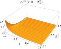
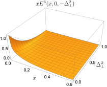
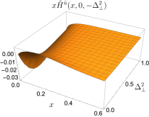
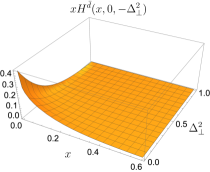
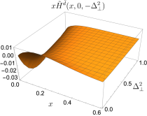
Figure 5: The sea quark chiral-even GPDs, $H^{\bar{q}}(x,0,-\Delta_{\perp}^{2})$ (left panel), $E^{\bar{q}}(x,0,-\Delta_{\perp}^{2})$ (middle panel), and $\tilde{H}^{\bar{q}}(x,0,-\Delta_{\perp}^{2})$ (right panel) plotted in the range $0.001<x<0.6$ at zero skewness for the proton calculated within our model. The upper panel is for the $\bar{u}$ quark and the lower panel represents the distributions for the $\bar{d}$ quark.

We utilize the obtained parameters listed in Table 1 in conjunction with the expressions from Eqs. (19) $-$ (21) to compute the sea quark GPDs in momentum space. We present three-dimensional (3D) plots for the three distributions, $xH^{\bar{q}}(x,0,-\Delta_{\perp}^{2})$, $xE^{\bar{q}}(x,0,-\Delta_{\perp}^{2})$, and $x\widetilde{H}^{\bar{q}}(x,0,-\Delta_{\perp}^{2})$ in Fig. 5. We observe that $xH^{\bar{q}}(x,0,-\Delta_{\perp}^{2})$ and $xE^{\bar{q}}(x,0,-\Delta_{\perp}^{2})$ exhibit similar behavior having positive peaks at low-$x$, whereas the distribution $x\widetilde{H}^{\bar{q}}(x,0,-\Delta_{\perp}^{2})$ shows distinctly different behavior from the other two GPDs, having negative peaks along the $\Delta_{\perp}^{2}$ direction at low-$x$. The maximum peak value for $xH^{\bar{q}}(x,0,-\Delta_{\perp}^{2})$ and $xE^{\bar{q}}(x,0,-\Delta_{\perp}^{2})$ occurs at the forward limit, $\Delta^{2}=0$. Notably, the largest peak for $E^{\bar{q}}(x,-\Delta_{\perp}^{2})$ is significantly larger than those for $H^{\bar{q}}(x,-\Delta_{\perp}^{2})$ and $\widetilde{H}^{\bar{q}}(x,-\Delta_{\perp}^{2})$. The maximum peak magnitude for $xH^{\bar{q}}(x,-\Delta_{\perp}^{2})$ is also larger than that of $x\widetilde{H}^{\bar{q}}(x,-\Delta_{\perp}^{2})$. We also notice that the magnitudes of all the distributions decrease as the momentum transfer $\Delta_{\perp}^{2}$ increases similar to that noticed for the quark GPDs in the nucleon Ji et al. (1997); Scopetta and Vento (2003); Petrov et al. (1998); Penttinen et al. (2000); Boffi et al. (2003, 2004); Vega et al. (2011); Mondal and Chakrabarti (2015); Chakrabarti and Mondal (2013b); Mondal (2017); de Teramond et al. (2018); Xu et al. (2021); Chakrabarti and Mondal (2013a). However, $xH^{\bar{q}}(x,0,-\Delta_{\perp}^{2})$ and $xE^{\bar{q}}(x,0,-\Delta_{\perp}^{2})$ fall faster than $x\widetilde{H}^{\bar{q}}(x,-\Delta_{\perp}^{2})$. The forward limits of $H^{\bar{q}}(x,0)$ and $\widetilde{H}^{\bar{q}}(x,0)$ correspond to ordinary helicity-independent and helicity-dependent sea quark PDFs, which are shown in Figs. 1 and 3, respectively.

Contrary to our model, where the $E^{\bar{q}}(x,0,-\Delta_{\perp}^{2})$ represents positive definite quantity for both the anti-up and anti-down quarks, which is consistent with the finding obtained in a light-cone baryon-meson fluctuation model Luan and Lu (2023), the covariant chiral effective theory He et al. (2022) displays a negative distribution for the anti-up quark but positive for the anti-down quark. It is anticipated that future investigations will employ theoretical and experimental analyses to examine the underlying causes of these discrepancies. We also notice that the magnitudes of the distributions in our model are comparable to those computed within the baryon-meson fluctuation model Luan and Lu (2023) but much higher than those results from the nonlocal covariant chiral effective theory He et al. (2022). It should also be noted that the scale of the baryon-meson fluctuation model, $Q_{0}\sim 0.7$ GeV, and the covariant chiral effective theory approach, $Q_{0}\sim 1.0$ GeV are different from model scale, $Q_{0}=2$ GeV. However, the qualitative nature of the distributions as shown in Refs. He et al. (2022); Luan and Lu (2023) aligns with our findings.

III.1 Flavor asymmetry at non zero momentum transfer

Turning now to the light sea quark asymmetry of the GPDs, in Figs. 6 and 7, we illustrate the distributions $xH^{\bar{d}-\bar{u}}(x,0,-\Delta_{\perp}^{2})$, $xE^{\bar{d}-\bar{u}}(x,0,-\Delta_{\perp}^{2})$, and $x\widetilde{H}^{\bar{d}-\bar{u}}(x,0,-\Delta_{\perp}^{2})$, which are known as the Electric, Magnetic, and Helicity flavor asymmetries, respectively. In Fig. 6, we show the 3D distributions in the region $0.005\leq x\leq 0.6$ and $0\leq\Delta_{\perp}^{2}\leq 1$ GeV², while in Fig. 7, we present the 2D sections of the distributions in the range $0.001\leq x\leq 0.6$ focusing on small-$x$ region for fixed momentum transfers. We observe that both the Electric and Magnetic asymmetries are negative in the range $0.001<x<0.005$ independent of choice of $\Delta_{\perp}^{2}$. This characteristic of the GPDs in our model is reassuring from Fig. 2, since the GPDs in forward limit reduce to PDFs. Both the asymmetries, on the other hand, are positive for $x>0.005$ with a peak at low-$x$ that decreases with increasing $\Delta_{\perp}^{2}$. At the peak, the magnetic GPD asymmetry $xE^{\bar{d}-\bar{u}}$ has magnitude $0.06$, which is about three times larger than that of the electric asymmetry $xH^{\bar{d}-\bar{u}}$. Note that these results are model and scale dependent. We predict them at the scale $Q_{0}=2$ GeV. The asymmetry behaviour may vary as it is evolved to different energy scales. Except in magnitude, both the asymmetries exhibit more or less similar behavior having their peaks around the same value of $x$ as can be seen in Fig. 7. These general properties should be nearly model-independent characteristics of the GPDs and, indeed, they are also observed in other theoretical study of the GPDs He et al. (2022). We also notice that in our model, both $xH^{\bar{d}-\bar{u}}$ and $xE^{\bar{d}-\bar{u}}$ fall off sharply with $\Delta_{\perp}^{2}$ and the distributions almost vanish for $x>0.6$, whereas the GPDs asymmetries reported in the nonlocal covariant chiral effective theory He et al. (2022) do not fall that fast. The third plots in Fig. 6 and 7 correspond to the asymmetry in the helicity distribution at different momentum transfer $\Delta_{\perp}^{2}$. We find that the distribution $x\widetilde{H}^{\bar{d}-\bar{u}}$ in our model changes its sign with $x$ and $\Delta_{\perp}^{2}$. This is similar to the finding reported by the HERMES Airapetian et al. (2004) when momentum transfer is zero.

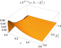
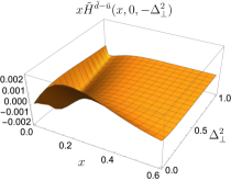
Figure 6: Flavor asymmetries for light sea quarks at finite momentum transfer, the electric asymmetry $xH^{\bar{d}-\bar{u}}$ (left panel), the magnetic asymmetry $xE^{\bar{d}-\bar{u}}$ (middle panel), and the helicity asymmetry $x\widetilde{H}^{\bar{d}-\bar{u}}$ (right panel) in the range $0.005<x<0.6$ and momentum transfer $0<\Delta_{\perp}^{2}<1$ GeV².

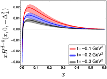
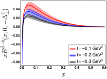
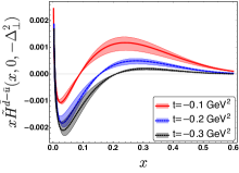
Figure 7: Two-dimensional plots of the sea quarks’ GPDs asymmetries $xH^{\bar{d}-\bar{u}}(x,0,-\Delta_{\perp}^{2})$ (left panel), $xE^{\bar{d}-\bar{u}}(x,0,-\Delta_{\perp}^{2})$ (middle panel), and $x\widetilde{H}^{\bar{d}-\bar{u}}(x,0,-\Delta_{\perp}^{2})$ (right panel) in the range $0.001<x<0.6$ with different values of momentum transfer $t=-\Delta_{\perp}^{2}$.

III.2 Sea quark orbital angular momentum

By exploring the GPDs associated with sea quarks, it becomes feasible to investigate the OAM contributions of the $\bar{u}$ and $\bar{d}$ quarks within the proton, which hold considerable importance in understanding the underlying characteristics of nucleon spin structure. Using the spin decomposition according to Ji Ji (1997b), the quark contribution can be separated further into the usual quark helicity and the gauge-invariant OAM,

$$L^{\bar{q}}=\int\text{d}x\,L^{\bar{q}}(x)\,,$$ (22)

where $L^{\bar{q}}(x)$ can be represented in terms of the chiral-even GPDs by the following relation

$$L^{\bar{q}}(x)=\frac{1}{2}\left\{x\left[H^{\bar{q}/P}(x,0,0)+E^{\bar{q}/P}(x,0,0)\right]-\widetilde{H}^{\bar{q}/P}(x,0,0)\right\}\,.$$ (23)

Figure 8 shows the $xL^{\bar{q}}(x)$ for both the up and down sea quarks. We find that the distributions are positive for all values of $x$, having a peak around $x\sim 0.15$. The distribution for the $\bar{d}$ is slightly larger than that of the $\bar{u}$ quark making the asymmetry $xL^{\bar{d}-\bar{u}}(x)$ small but positive. It vanishes after $x$ increases over $0.6$.

It is expected that the sea quarks do not contribute much to the OAM of the proton but it also depends on the region of $x$. Since there are more sea quarks involved in the lower-$x$ region, therefore, the result of the OAM $L^{\bar{q}}$ depends on the limit of $x$ in the Eq. (22). In the region, $0.001<x<1$, our model provides

$$L^{\bar{u}}=0.040\pm 0.003,~{}~{}~{}~{}L^{\bar{d}}=0.048\pm 0.002,$$ (24)

while in the region $0.01<x<1$, we obtain

$$L^{\bar{u}}=0.035\pm 0.003,~{}~{}~{}~{}L^{\bar{d}}=0.044\pm 0.002,$$ (25)

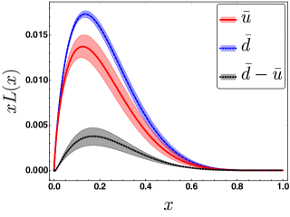
Figure 8: The sea quark OAM distribution, $xL(x)$, for $\bar{d}$ (blue line with blue band) and $\bar{u}$ (red line with red band) and their asymmetry $xL^{\bar{d}-\bar{u}}(x)$ (black line with black band) in the proton evaluated within our model.

IV Sea quark TMDs

TMDs encode three-dimensional momentum information of a parton inside a hadron. TMDs are able to describe a wide range of phenomena following QCD factorization theorems Barone et al. (2010); Collins et al. (1989). They are essential in order to characterise the SIDIS or the Drell-Yan processes Collins et al. (1985), where the collinear picture of the parton model fails. The quark TMDs are parameterization factors of the quark correlation function Goeke et al. (2005); Meissner et al. (2007)

$$\Phi^{\Gamma}(x,{\bf k}_{\perp};P,S)=\frac{1}{xP^{+}}\int\frac{\text{d}\xi^{-}}{2\pi}\,\frac{\text{d}^{2}\mathbf{\xi}{{}_{\perp}}}{(2\pi)^{2}}\,e^{ik\cdot\xi}\,\langle P,S\lvert\bar{\psi}(0)\mathcal{W}(0,\,\xi)\Gamma\psi(\xi)\rvert P,S\rangle\bigg{\rvert}_{\xi^{+}=0}\,,$$ (26)

where, $\psi$ represents the quark field, and $\Gamma$ is the Dirac matrix, which in the leading twist, is taken as $\Gamma\equiv\gamma^{+}$, $\gamma^{+}\gamma^{5}$, $i\sigma^{j+}\gamma^{5}$.

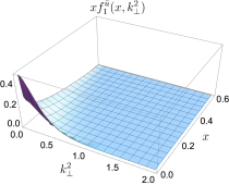
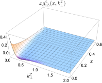
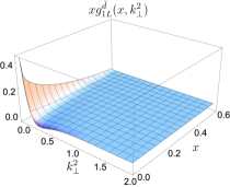
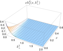
Figure 9: The sea quark T-even TMDs, $x{f}^{\bar{q}}_{1}(x,{\bf k}_{\perp}^{2})$ (left panel), $x{g}^{\bar{q}}_{1L}(x,{\bf k}_{\perp}^{2})$ (middle panel), and $xh_{1}^{\bar{q}}(x,{\bf k}_{\perp}^{2})$ (right panel) calculated in the range $0.001<x<0.6$ and momentum transfer $0<{\bf k}_{\perp}^{2}<2$ GeV² in the proton within our model. The upper panel is for the $\bar{u}$ quark and the lower panel represents the distributions for the $\bar{d}$ quark. ${\bf k}_{\perp}^{2}$ is in units of GeV².

It turns out that, at the leading twist there are eight quark TMDs for the nucleon. They are parameterized as follows  Goeke et al. (2005); Meissner et al. (2007):

$$\Phi^{[\gamma^{+}]}(x,\mathbf{k}_{\perp};\mathbf{S})=f_{1}^{q}-\frac{\epsilon_{\perp}^{ij}k_{\perp}^{i}S_{\perp}^{j}}{m}f_{1T}^{\perp q}\;,$$ (27)

$$\Phi^{[\gamma^{+}\gamma^{5}]}(x,\mathbf{k}_{\perp};\mathbf{S})=S_{z}g_{1L}^{q}+\frac{\mathbf{k}_{\perp}\cdot\mathbf{S}_{\perp}}{m}g_{1T}^{q}\;,$$ (28)

$$\Phi^{[i\sigma^{j+}\gamma^{5}]}(x,\mathbf{k}_{\perp};\mathbf{S})=S_{\perp}^{j}h_{1}^{q}+S_{z}\frac{k^{j}_{\perp}}{m}h_{1L}^{\perp q}+S^{i}_{\perp}\frac{2k_{\perp}^{i}k_{\perp}^{j}-\mathbf{k}_{\perp}^{2}\delta^{ij}}{2m^{2}}h_{1T}^{\perp q}+\frac{\epsilon_{\perp}^{ji}k_{\perp}^{i}}{m}h_{1}^{\perp q}\;,$$ (29)

where $h_{1}^{q}:\,=h_{1T}^{q}+\frac{\mathbf{k}_{\perp}^{2}}{2m^{2}}h_{1T}^{\perp q}$ and we use the convention $\epsilon^{12}=1$. We choose a frame in which the incoming proton has zero transverse momentum i.e. $P=(P^{+},\mathbf{0}_{\perp},P^{-})$ and the spin four vector such that $P\cdot S=0$ and $S^{2}=-1$. The covariant four-vector $S$ can be represented by the three-vector $\mathbf{S}:\,=(\perp{S},S_{z})$, with $\mathbf{S}^{2}=1$.

In the current study, we only retain the zeroth-order expansion of the gauge link. Note that $f_{1T}^{\perp}$ and $h_{1}^{\perp}$, are T-odd distributions and vanish under the zeroth-order expansion of the gauge link, i.e., $\mathcal{W}(0,\,\xi)=1$ in Eq. (26). All six T-even leading-twist TMDs can be expressed in terms of the LFWFs in our model as Bacchetta et al. (2016),

$${f}^{\bar{q}}_{1}(x,{\bf k}_{\perp}) = \frac{1}{16\pi^{3}}\biggl{[}|\psi^{\uparrow}_{\bar{q};+\frac{1}{2}}(x,{\bf k}_{\perp})|^{2}+|\psi^{\uparrow}_{\bar{q};-\frac{1}{2}}(x,{\bf k}_{\perp})|^{2}\biggr{]}\,,$$ (30)

$${g}^{\bar{q}}_{1L}(x,{\bf k}_{\perp}) = \frac{1}{16\pi^{3}}\biggl{[}|\psi^{\uparrow}_{\bar{q};+\frac{1}{2}}(x,{\bf k}_{\perp})|^{2}-|\psi^{\uparrow}_{\bar{q};-\frac{1}{2}}(x,{\bf k}_{\perp})|^{2}\biggr{]}\,,$$ (31)

$$g_{1T}^{\bar{q}}(x,\textbf{k}_{\perp}^{2}) = \frac{M}{2(2\pi)^{3}{\bf k}_{\perp}^{2}}\bigg{[}k_{R}\psi^{\uparrow\dagger}_{\bar{q},+\frac{1}{2}}(x,\textbf{k}_{\perp})\psi^{\downarrow}_{\bar{q},+\frac{1}{2}}(x,\textbf{k}_{\perp})+k_{L}\psi^{\downarrow\dagger}_{\bar{q},+\frac{1}{2}}(x,\textbf{k}_{\perp})\psi^{\uparrow}_{\bar{q},+\frac{1}{2}}(x,\textbf{k}_{\perp})\bigg{]}\,,$$ (32)

$$h_{1L}^{\perp\bar{q}}(x,\textbf{k}_{\perp}^{2}) = \frac{M}{2(2\pi)^{3}{\bf k}_{\perp}^{2}}\bigg{[}k_{R}\psi^{\uparrow\dagger}_{\bar{q},-\frac{1}{2}}(x,\textbf{k}_{\perp})\psi^{\uparrow}_{\bar{q},+\frac{1}{2}}(x,\textbf{k}_{\perp})+k_{L}\psi^{\uparrow\dagger}_{\bar{q},+\frac{1}{2}}(x,\textbf{k}_{\perp})\psi^{\uparrow}_{\bar{q},-\frac{1}{2}}(x,\textbf{k}_{\perp})\bigg{]}\,,$$ (33)

$$h_{1T}^{\perp\bar{q}}(x,\textbf{k}_{\perp}^{2}) = \frac{M}{2(2\pi)^{3}{\bf k}_{\perp}^{4}}\bigg{[}k_{R}^{2}\psi^{\uparrow\dagger}_{\bar{q},-\frac{1}{2}}(x,\textbf{k}_{\perp})\psi^{\downarrow}_{\bar{q},+\frac{1}{2}}(x,\textbf{k}_{\perp})+k_{L}^{2}\psi^{\downarrow\dagger}_{\bar{q},+\frac{1}{2}}(x,\textbf{k}_{\perp})\psi^{\uparrow}_{\bar{q},-\frac{1}{2}}(x,\textbf{k}_{\perp})\bigg{]}\,,$$ (34)

$$h_{1}^{\bar{q}}(x,\textbf{k}_{\perp}^{2}) = \frac{1}{2(2\pi)^{3}}\psi^{\uparrow\dagger}_{\bar{q},+\frac{1}{2}}(x,\textbf{k}_{\perp})\psi^{\downarrow}_{\bar{q},-\frac{1}{2}}(x,\textbf{k}_{\perp})\,,$$ (35)

where $k_{R/L}=k_{1}\pm ik_{2}$ are defined in terms of the components of the transverse momentum. Utilizing the explicit form of the LFWFs, Eq. (5), we derive the following expressions of the sea quark T-even TMDs within our model,

$${f}^{q}_{1}(x,{\bf k}_{\perp}^{2}) = \frac{1}{\pi\kappa^{2}}\biggl{[}1+\frac{{\bf k}_{\perp}^{2}}{\kappa^{2}}\biggr{]}Ax^{2\alpha-1}(1-x)^{6+2\beta}\log(1/1-x)\exp{\bigg{[}-\frac{\log[1/(1-x)]}{\kappa^{2}x(1-x)}{\bf k}_{\perp}^{2}\bigg{]}}\,,$$ (36)

$${g}^{q}_{1L}(x,{\bf k}_{\perp}^{2}) = \frac{1}{\pi\kappa^{2}}\biggl{[}1-\frac{{\bf k}_{\perp}^{2}}{\kappa^{2}}\biggr{]}Ax^{2\alpha-1}(1-x)^{6+2\beta}\log(1/1-x)\exp{\bigg{[}-\frac{\log[1/(1-x)]}{\kappa^{2}x(1-x)}{\bf k}_{\perp}^{2}\bigg{]}}\,,$$ (37)

$${g}^{q}_{1T}(x,{\bf k}_{\perp}^{2}) = \frac{1}{\pi\kappa^{2}}\frac{2M}{\kappa}Ax^{2\alpha-1}(1-x)^{6+2\beta}\log(1/1-x)\exp{\bigg{[}-\frac{\log[1/(1-x)]}{\kappa^{2}x(1-x)}{\bf k}_{\perp}^{2}\bigg{]}}$$ (38)

$${h}^{q\perp}_{1L}(x,{\bf k}_{\perp}^{2}) = -\frac{1}{\pi\kappa^{2}}\frac{2M}{\kappa}Ax^{2\alpha-1}(1-x)^{6+2\beta}\log(1/1-x)\exp{\bigg{[}-\frac{\log[1/(1-x)]}{\kappa^{2}x(1-x)}{\bf k}_{\perp}^{2}\bigg{]}}\,,$$ (39)

$${h}^{q\perp}_{1T}(x,{\bf k}_{\perp}^{2}) = -\frac{1}{\pi\kappa^{2}}\frac{2M^{2}}{\kappa^{2}}Ax^{2\alpha-1}(1-x)^{6+2\beta}\log(1/1-x)\exp{\bigg{[}-\frac{\log[1/(1-x)]}{\kappa^{2}x(1-x)}{\bf k}_{\perp}^{2}\bigg{]}}\,,$$ (40)

$${h}^{q}_{1}(x,{\bf k}_{\perp}^{2}) = \frac{1}{\pi\kappa^{2}}Ax^{2\alpha-1}(1-x)^{6+2\beta}\log(1/1-x)\exp{\bigg{[}-\frac{\log[1/(1-x)]}{\kappa^{2}x(1-x)}{\bf k}_{\perp}^{2}\bigg{]}}\,.$$ (41)

The 3D structures of the six leading-twist sea quark TMDs in our model are shown in Figs. 9 and 10. We present the three T-even TMDs: $f_{1}^{\bar{q}}(x,{\bf k}_{\perp}^{2})$, $g_{1L}^{\bar{q}}(x,{\bf k}_{\perp}^{2})$, and $h_{1}^{\bar{q}}(x,{\bf k}_{\perp}^{2})$, which have their colinear limits, shown in Fig. 1, 3, and 4, respectively. The other three TMDs: $g_{1T}^{\bar{q}}(x,{\bf k}_{\perp}^{2})$, $h_{1L}^{\bar{q}}(x,{\bf k}_{\perp}^{2})$, and $h_{1T}^{\bar{q}}(x,{\bf k}_{\perp}^{2})$ are illustrated in Fig. 10. It is clearly seen there that all six nonzero TMDs have peaks near $(x,{\bf k}_{\perp}^{2})\to(0,0)$. These peaks designate the dominant probability is to find a light sea quark in the proton in each of the different polarization configurations. The $xf_{1}^{\bar{q}}$, $xg_{1L}^{\bar{q}}$, $xh_{1}^{\bar{q}}$, and $xg_{1T}^{\bar{q}}$ show positive distributions and they appear very similar by eye, the peak in the longitudinal direction runs higher with decreasing ${\bf k}_{\perp}^{2}$ but falls rapidly to zero after ${\bf k}_{\perp}^{2}$ increases above $1$ GeV². Meanwhile, the peak in the transverse direction falls to zero when $x$ increases above $0.6$. We also notice that $xg_{1L}^{\bar{q}}(x,{\bf k}_{\perp}^{2})$ shows slightly negative distribution for the region $0.2~{}{\rm GeV}^{2}<{\bf k}_{\perp}^{2}<1.0~{}{\rm GeV}^{2}$ at very low-$x$. This TMD after integrating out the momenta quantifies the amount of spin contribution of the sea quarks in the proton. In this particular model, the TMDs corresponding to transversely polarized quarks within a longitudinally polarized proton, denoted by ${h}^{q\perp}_{1L}(x,{\bf k}_{\perp}^{2})$ and a transversely polarized proton, denoted by ${h}^{q\perp}_{1T}(x,{\bf k}_{\perp}^{2})$ are negative for both the anti-up and anti-down quarks.The negative trend of ${h}^{\bar{q}\perp}_{1L}$ for both the anti-up and the anti-down quarks is similar to the valence up and down quarks Maji and Chakrabarti (2017), while the ${h}^{\bar{q}\perp}_{1T}$ distribution for the sea quarks doesn’t follow the same trend as in the case of valence quarks. Our model predicts negative pretzelosity for both the anti-up and the anti-down quarks.

The features of all the anti-up quark TMDs are very similar to those for the anti-down quark. However, we also find that there exists the flavor asymmetries in the transverse momentum plane, as can be seen from Fig. 11. The asymmetry distributions $xf_{1}^{\bar{d}-\bar{u}}$, $xg_{1L}^{\bar{d}-\bar{u}}$, and $xh_{1}^{\bar{d}-\bar{u}}$ are found to be very similar in our model having a peak around $(x,{\bf k}_{\perp}^{2})=(0.03,0)$ but falls rapidly to zero with increasing ${\bf k}_{\perp}^{2}$. Note that the ($\bar{d}-\bar{u}$) TMD asymmetries are negative at low-$x$ independent of choice of ${\bf k}_{\perp}^{2}$, indicating the density of anti-up quark is larger than that of the anti-down quark at very small-$x$ domain, which is also observed in the PDFs and the GPDs asymmetries in Figs. 2 and  7, respectively.

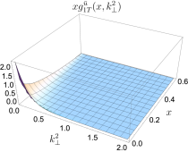
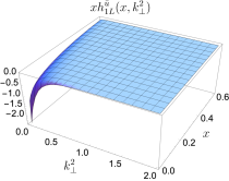
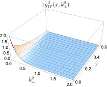
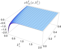
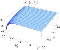
Figure 10: The sea quark T-even TMDs, $x{g}^{\bar{q}}_{1T}(x,{\bf k}_{\perp}^{2})$, $x{h}^{\bar{q}}_{1L}(x,{\bf k}_{\perp}^{2})$, and $xh_{1T}^{\bar{q}}(x,{\bf k}_{\perp}^{2})$ calculated in the range $0.001<x<0.6$ and momentum transfer $0<{\bf k}_{\perp}^{2}<2$ GeV² in the proton within our model. The upper panel is for the $\bar{u}$ quark and the lower panel represents the distributions for the $\bar{d}$ quark. ${\bf k}_{\perp}^{2}$ is in units of GeV².

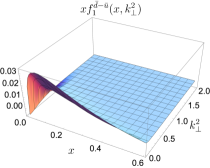
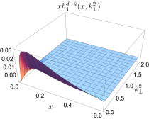
Figure 11: TMD asymmetries of light sea quarks in the proton, $xf_{1}^{\bar{d}-\bar{u}}$ (left plot), $xg_{1L}^{\bar{d}-\bar{u}}$ (middle plot), and $xh_{1}^{\bar{d}-\bar{u}}$ (right plot) calculated in the range $0.005<x<0.6$ and momentum transfer $0<{\bf k}_{\perp}^{2}<2$ GeV² in the proton within our model. ${\bf k}_{\perp}^{2}$ is in units of GeV².

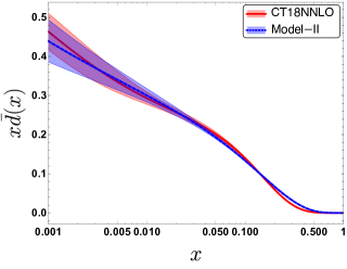
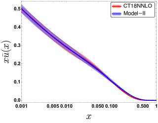
Figure 12: The sea quark unpolarized distributions in the proton, left panel: $x{\bar{d}}(x)$ and right panel: $x{\bar{u}}(x)$ as a function of longitudinal momentum fraction $x$ in the kinematics region $0.001\leq x\leq 1$ at $Q_{0}=2$ GeV. Our model results (dashed-blue lines with blue bands) are compared with the CTEQ18 NNLO dataset (solid-red lines with red bands) Hou et al. (2021)

.

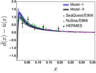
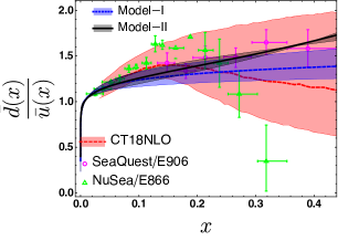
Figure 13: The comparison of light flavor sea asymmetries in the proton between the Model-I (blue lines with blue bands) and Model-II (black lines with black bands), left panel: $\bar{d}(x)-\bar{u}(x)$ and right panel: $\bar{d}(x)/\bar{u}(x)$ as a function of $x$. Our results are compared with the experimental data from the SeaQuest/E906 Dove et al. (2023) (magenta points), NuSea/E866 Towell et al. (2001) (green points), and HERMES Ackerstaff et al. (1998)(black points) Collaborations. In the right panel, we also include the CTEQ18 NLO global analysis Hou et al. (2021) (blue line with blue band) for the comparison.

V Model-II

For further investigation of the model dependency in the flavor asymmetry, instead of choosing Eq. (5) in our light-front spectator model, we use a different form of the wave function adopted from a phenomenological model discussed in Ref. Brodsky et al. (2022),

$$\varphi(x,{\bf k}_{\perp}^{2})=\sqrt{A}\frac{4\pi}{\kappa}\sqrt{\frac{\log[1/(1-x)]}{x}}x^{\alpha}(1-x)^{3+\beta}\exp{\bigg{[}-\frac{{\bf k}_{\perp}^{2}}{2\kappa^{2}}\bigg{]}}.$$ (42)

We refer this model as Model-II.

Table 3: Fitted parameters for Model-II at $Q_{0}=2$ GeV.

	A	$\alpha$	$\beta$
$\overline{d}$	$0.162_{0.015}^{-0.012}$	$-0.572_{0.015}^{-0.014}$	$-0.253_{0.164}^{-0.133}$
$\overline{u}$	$0.116_{-0.01}^{0.009}$	$-0.606_{-0.003}^{0.002}$	$-0.022_{-0.004}^{0.004}$

V.1 PDFs

In this particular model, the unpolarized sea quark PDF reads

$$f_{1}^{\bar{q}}(x) = \int\frac{\text{d}^{2}{\bf k}_{\perp}}{16\pi^{3}}\,\biggl{[}|\psi^{\uparrow}_{\bar{q};+\frac{1}{2}}(x,{\bf k}_{\perp})|^{2}+|\psi^{\uparrow}_{\bar{q};-\frac{1}{2}}(x,{\bf k}_{\perp})|^{2}\biggr{]}$$ (43)

$$= 2Ax^{2\alpha-1}(1-x)^{6+2\beta}\log\left(\frac{1}{1-x}\right),$$

while the helicity PDF $g_{1L}(x)$ vanishes. We fit $f_{1}^{\bar{q}}(x)$ with the CT18NNLO data at $Q_{0}=2$ GeV and obtain a different set of the model parameters, $\alpha$, $\beta$, and $A$ given in Table 3. The results of the fits for $x{\bar{q}}(x)$ are shown in Fig. 12. The value of $\chi^{2}$/d.o.f. for the fits of the $x{\bar{d}}(x)$ and $x{\bar{u}}(x)$ are $0.2530$ and $0.0234$, respectively in the region $0.001<x<0.1$.

Figure 13 compares the flavor asymmetries between between the Model-I (using Eq. (5) and parameters listed in Table 1) and the Model-II. We find that the ${\bar{d}}(x)-{\bar{u}}(x)$ asymmetry in both models is almost identical. However, for the ${\bar{d}}(x)/{\bar{u}}(x)$ asymmetry, the Model-II describes the growth trend toward higher $x$ of the latest experimental data from the SeaQuest/E906 Collaboration  Dove et al. (2023) better than the Model-I.

V.2 GPDs and OAM

The GPDs can be evaluated following the similar procedure as described in Eqs. (14) to (16) for the Model-I. Using the light-front wave functions, the explicit expressions of the sea quark GPDs at zero skewness in the Model-II read

$$H^{\bar{q}}(x,0,-\Delta_{\perp}^{2}) = 2Ax^{2\alpha-1}(1-x)^{6+2\beta}\log\left(\frac{1}{1-x}\right)\left(1-\frac{\Delta_{\perp}^{2}(1-x)^{2}}{4\kappa^{2}}\right)\exp{\bigg{[}-\frac{(1-x)^{2}}{4\kappa^{2}}\Delta_{\perp}^{2}\bigg{]}}\,,$$ (44)

$$E^{\bar{q}}(x,0,-\Delta_{\perp}^{2}) = \frac{M_{N}}{\kappa}2Ax^{2\alpha-1}(1-x)^{7+2\beta}\exp{\bigg{[}-\frac{(1-x)^{2}}{4\kappa^{2}}\Delta_{\perp}^{2}\bigg{]}}\,,$$ (45)

$$\tilde{H}^{q}(x,0,-\Delta_{\perp}^{2}) = 0\,.$$ (46)

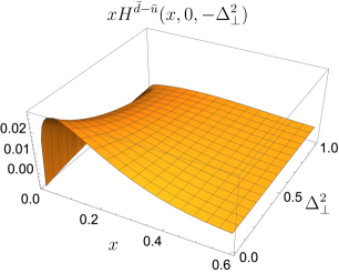
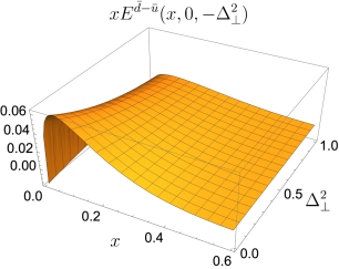
Figure 14: The electric $xH^{\bar{d}-\bar{u}}$ (left plot) and magnetic $xE^{\bar{d}-\bar{u}}$ (right plot) GPDs asymmetry in the range $0.005<x<0.6$ and the momentum transfer $0<\Delta_{\perp}^{2}<1$ from Model-II.

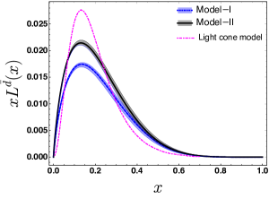
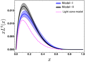
Figure 15: Comparison of the sea quark OAM distributions, $xL^{\bar{q}}(x)$, among the Model-I, the Model-II, and a light-cone model Luan and Lu (2023). The left plot is for the $\bar{d}$ quark and the right plot is for the $\bar{u}$ quark.

Figure 14 presents the qualitative behavior of $xH^{\bar{d}-\bar{u}}(x,0,-\Delta_{\perp}^{2})$ and $xE^{\bar{d}-\bar{u}}(x,0,-\Delta_{\perp}^{2})$ computed using the Model-II. The distributions are plotted in the region $0.005<x<0.6$ and $0<\Delta_{\perp}^{2}<1.0$ GeV². We observe that there is not much difference in magnitude of the peaks compared to that in the Model-I (Fig. 6) but with increasing $x$ and $\Delta_{\perp}^{2}$, the behaviors are quite different between these two models. The asymmetries in the Model-I fall faster than the Model-II. We find that Model-II provides compatible behaviour of the distributions $xH^{\bar{d}-\bar{u}}(x,0,-\Delta_{\perp}^{2})$ and $xE^{\bar{d}-\bar{u}}(x,0,-\Delta_{\perp}^{2})$ as observed in non-local covariant chiral effective theory He et al. (2022).

Table 4: The Kinetic OAM, helicity and total angular momentum of up and down sea quarks in Model-I, Model-II and a Light cone model Luan and Lu (2023).

	$L^{\bar{u}}$	$L^{\bar{d}}$	$\Delta\Sigma^{\bar{u}}/2$	$\Delta\Sigma^{\bar{d}}/2$	$J^{\bar{u}}=L^{\bar{u}}+\Delta\Sigma^{\bar{u}}/2$	$J^{\bar{d}}=L^{\bar{d}}+\Delta\Sigma^{\bar{d}}/2$
Model-I	$0.040\pm 0.003$	$0.048\pm 0.002$	$0.013\pm 0.001$	$0.015\pm 0.001$	$0.053\pm 0.004$	$0.063\pm 0.003$
Model-II	$0.048\pm 0.003$	$0.059\pm 0.002$	0.00	0.00	$0.048\pm 0.003$	$0.059\pm 0.002$
Light cone model Luan and Lu (2023)	$0.025$	$0.046$	0.00	0.00	$0.025$	$0.046$

Figure 15 compares the distribution $xL^{\bar{q}}(x)$ between light cone model Luan and Lu (2023), the Model-I and the Model-II for both the down and up sea quarks. The qualitative nature of the distribution is more or less same in these three models except the magnitude in the light-cone model. Table 4 displays our predictions for the up and down sea quarks’ OAM, spin, and total angular momentum. These results are evaluated within the region $0.001<x<1$ for the Model-I and Model-II. We observe that the down sea quark contributes more to the proton spin than the up sea quark. The spin contribution vanishes in the Model-II and the light-cone model Luan and Lu (2023). The total angular momentum in the Model-I is higher than the Model-II and the light-one model for both sea quarks. While the down quark’s kinetic OAM is comparable in the Model-I and the light cone model, the up quark’s kinetic OAM is comparable in the Model-I and the Model-II.

V.3 TMDs

Employing the light-front wave functions, we also calculate the sea quark TMDs in the Model-II. The unpolarized TMD in this particular model is expressed as

$${f}^{q}_{1}(x,{\bf k}_{\perp}^{2}) = \frac{1}{\pi\kappa^{2}}Ax^{2\alpha-1}(1-x)^{6+2\beta}\log(1/1-x)\left(1+\frac{{\bf k}_{\perp}^{2}}{\kappa^{2}}\right)\exp{\left[-\frac{{\bf k}_{\perp}^{2}}{\kappa^{2}}\right]}\,.$$ (47)

The flavor asymmetry in TMD within the Model-II is shown in Fig. 16. Here again, we notice that the qualitative nature of $xf_{1}^{\bar{d}-\bar{u}}(x,{\bf k}_{\perp}^{2})$ in the Model-II is more or less same as observed in the Model-I (Fig. 11). The magnitude of the peak is comparable to that in Model-I but with increasing ${\bf k}_{\perp}^{2}$, the asymmetries in the Model-II fall much slower than the Model-I.

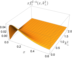
Figure 16: Flavor asymmetry in the TMD, $xf_{1}^{\bar{d}-\bar{u}}(x,{\bf k}_{\perp}^{2})$ calculated in the range $0.005<x<0.6$ and momentum transfer $0<{\bf k}_{\perp}^{2}<2$ GeV² in the proton within Model-II.

VI Summary and Outlook

In this work, we have studied the flavor asymmetries of the light sea quarks within the proton by employing a light-front spectator model, where the sea quarks are viewed as active partons and the remaining components of the proton are considered as the spectator. We have formulated this model based on the light-front wave function modelled by the soft wall AdS/QCD and parameterized by fitting the unpolarized parton distribution functions (PDFs) of light sea quarks from the CTEQ18 NNLO global analysis at the scale $Q_{0}=2$ GeV. We have calculated the sea quark leading-twist PDFs, generalized parton distributions (GPDs), and transverse momentum dependent parton distribution functions (TMDs) and their flavor asymmetries. We have observed that at small-$x$ ($<0.01$), ${\bar{u}}(x)$ is larger than ${\bar{d}}(x)$ in our model. The ${\bar{d}}(x)-{\bar{u}}(x)$ asymmetry agrees well with the available experimental data from the NuSea/E866, HERMES, and SeaQuest/E906 Collaborations Towell et al. (2001); Ackerstaff et al. (1998); Dove et al. (2023). From the comparison between the model and the experiments, we have found that our model describes well the trend of the latest experimental data of the ${\bar{d}}(x)/{\bar{u}}(x)$ asymmetry from the the SeaQuest/E906 Collaboration Dove et al. (2023), however fails to explain the overall behavior shown by NuSea/E866 data Towell et al. (2001). Similar results are also observed in the pion model Choudhary et al. (2023); Alberg et al. (2022) and the chiral light-front perturbation theory Alberg and Miller (2019). Our model leads to more or less satisfactory results for the sea quark helicity PDFs when we compare with the experimental data from the COMPASS Alekseev et al. (2010) and the HERMES Airapetian et al. (2004). It should be noted that the signs of sea quark helicity PDFs are not fixed by the experiments.

We have presented results for the sea quark unpolarized and helicity-dependent GPDs of the proton in momentum space for zero skewness and we found that the qualitative behavior of the GPD asymmetries in our model bears similarities to other phenomenological models He et al. (2022); Luan and Lu (2023). We have employed these GPDs to study the orbital angular momentum (OAM) distribution at the density level. Within our model, we have found that the $\bar{d}$ quark distribution dominates over the $\bar{u}$ quark distribution and their qualitative features are in accord with the behavior observed in a light-front baryon-meson fluctuation model Luan and Lu (2023). We have obtained that the sea quark OAMs, $L^{\bar{u}}=0.040\pm 0.003$ and $L^{\bar{d}}=0.048\pm 0.002$ strongly dominate over their spin contributions, $\Delta\Sigma^{\bar{u}}/2=0.013\pm 0.001$ and $\Delta\Sigma^{\bar{d}}/2=0.015\pm 0.001$.

We have further investigated the leading-twist TMDs of the sea quarks within the proton. In this study, the gauge link has been set to unity, which leaves us six nonzero T-even TMDs out of the eight leading-twist TMDs. We have observed that the properties of all nonzero TMDs for both the $\bar{u}$ and $\bar{d}$ are are very similar. They have peaks at $(x,{\bf k}_{\perp}^{2})\to(0,0)$ and fall rapidly as $x$ and ${\bf k}_{\perp}^{2}$ increase. It is not surprising since the sea quark density is much higher at small-$x$ domain. The sea asymmetry in the TMDs has been observed only when ${\bf k}_{\perp}^{2}$ is small ($<0.2$ GeV²) for all values of $x$. For further investigation of the model dependency of the sea quark properties, we have considered a different form of the light-front wave function (Model-II) and studied those asymmetries in this model. We have noticed that this model shows more or less similar characteristics of the sea quarks as observed in the Model-I.

The proposed light-front spectator models can be further employed to compute the other properties of the sea quarks, such as the chiral-odd GPDs, T-odd TMDs, and Wigner distributions, etc., in the proton as well as to study the role of sea quarks in the single and double spin asymmetries. The present calculation can be straightforwardly extended to investigate the strange and the charm flavor asymmetries in the proton.

References

- Brodsky et al. (1980) S. J. Brodsky, P. Hoyer, C. Peterson, and N. Sakai, Phys. Lett. B 93, 451 (1980).
- Brodsky et al. (1981) S. J. Brodsky, C. Peterson, and N. Sakai, Phys. Rev. D 23, 2745 (1981).
- Drell and Yan (1971) S. D. Drell and T.-M. Yan, Annals Phys. 66, 578 (1971).
- Chang and Peng (2014) W.-C. Chang and J.-C. Peng, Prog. Part. Nucl. Phys. 79, 95 (2014), eprint 1406.1260.
- Buccella and Soffer (1993) F. Buccella and J. Soffer, EPL 24, 165 (1993).
- Kumano (1998) S. Kumano, Phys. Rept. 303, 183 (1998), eprint hep-ph/9702367.
- Gottfried (1967) K. Gottfried, Phys. Rev. Lett. 18, 1174 (1967).
- Amaudruz et al. (1991) P. Amaudruz et al. (New Muon), Phys. Rev. Lett. 66, 2712 (1991).
- Arneodo et al. (1994) M. Arneodo et al. (New Muon), Phys. Rev. D 50, R1 (1994).
- Kumano (1991) S. Kumano, Phys. Rev. D 43, 3067 (1991).
- Wakamatsu (2014) M. Wakamatsu, Phys. Rev. D 90, 034005 (2014), eprint 1405.7095.
- Lin et al. (2015) H.-W. Lin, J.-W. Chen, S. D. Cohen, and X. Ji, Phys. Rev. D 91, 054510 (2015), eprint 1402.1462.
- Song et al. (2011) H. Song, X. Zhang, and B.-Q. Ma, Eur. Phys. J. C 71, 1542 (2011), eprint 1101.3378.
- Brodsky et al. (2022) S. J. Brodsky, V. E. Lyubovitskij, and I. Schmidt, Phys. Rev. D 106, 094025 (2022), eprint 2209.00403.
- Garvey and Peng (2001) G. T. Garvey and J.-C. Peng, Prog. Part. Nucl. Phys. 47, 203 (2001), eprint nucl-ex/0109010.
- Dove et al. (2023) J. Dove et al. (FNAL E906, SeaQuest), Phys. Rev. C 108, 035202 (2023), eprint 2212.12160.
- Accardi et al. (2020) A. Accardi, C. E. Keppel, S. Li, W. Melnitchouk, G. Niculescu, I. Niculescu, and J. F. Owens (CTEQ-Jefferson Lab (CJ)), Phys. Lett. B 801, 135143 (2020), eprint 1910.02931.
- Kotlorz et al. (2021) A. Kotlorz, D. Kotlorz, and O. V. Teryaev, Int. J. Mod. Phys. A 36, 2150254 (2021).
- Hawker et al. (1998) E. A. Hawker et al. (NuSea), Phys. Rev. Lett. 80, 3715 (1998), eprint hep-ex/9803011.
- Peng et al. (1998) J. C. Peng et al. (NuSea), Phys. Rev. D 58, 092004 (1998), eprint hep-ph/9804288.
- Dove (2020) J. Dove, Ph.D. thesis, Illinois U., Urbana (2020).
- Nagai (2019) K. Nagai (SeaQuest), JPS Conf. Proc. 26, 021011 (2019).
- McGaughey et al. (1992) P. L. McGaughey et al., Phys. Rev. Lett. 69, 1726 (1992).
- Choudhary et al. (2023) S. Choudhary, P. Srivastava, and H. Dahiya (2023), eprint 2303.11744.
- Dorokhov and Kochelev (1991) A. E. Dorokhov and N. I. Kochelev, Phys. Lett. B 259, 335 (1991).
- Dorokhov and Kochelev (1993) A. E. Dorokhov and N. I. Kochelev, Phys. Lett. B 304, 167 (1993).
- Trevisan et al. (2008) L. A. Trevisan, C. Mirez, T. Frederico, and L. Tomio, Eur. Phys. J. C 56, 221 (2008).
- He et al. (2022) F. He, C.-R. Ji, W. Melnitchouk, A. W. Thomas, and P. Wang, Phys. Rev. D 106, 054006 (2022), eprint 2202.00266.
- Rojo et al. (2015) J. Rojo et al., J. Phys. G 42, 103103 (2015), eprint 1507.00556.
- Harland-Lang et al. (2015) L. A. Harland-Lang, A. D. Martin, P. Motylinski, and R. S. Thorne, Eur. Phys. J. C 75, 204 (2015), eprint 1412.3989.
- Accardi et al. (2016) A. Accardi et al., Eur. Phys. J. A 52, 268 (2016), eprint 1212.1701.
- Abdul Khalek et al. (2022) R. Abdul Khalek et al., Nucl. Phys. A 1026, 122447 (2022), eprint 2103.05419.
- Anderle et al. (2021) D. P. Anderle et al., Front. Phys. (Beijing) 16, 64701 (2021), eprint 2102.09222.
- Cao (2016) F. G. Cao, Int. J. Mod. Phys. Conf. Ser. 40, 1660020 (2016).
- He and Wang (2018) F. He and P. Wang, Phys. Rev. D 97, 036007 (2018), eprint 1711.05896.
- Lyubovitskij and Schmidt (2023) V. E. Lyubovitskij and I. Schmidt, JHEP 05, 054 (2023), [Erratum: JHEP 08, 061 (2023)], eprint 2212.04340.
- Sufian et al. (2020) R. S. Sufian, T. Liu, A. Alexandru, S. J. Brodsky, G. F. de Téramond, H. G. Dosch, T. Draper, K.-F. Liu, and Y.-B. Yang, Phys. Lett. B 808, 135633 (2020), eprint 2003.01078.
- Towell et al. (2001) R. S. Towell et al. (NuSea), Phys. Rev. D 64, 052002 (2001), eprint hep-ex/0103030.
- Dove et al. (2021) J. Dove et al. (SeaQuest), Nature 590, 561 (2021), [Erratum: Nature 604, E26 (2022)], eprint 2103.04024.
- Ackerstaff et al. (1998) K. Ackerstaff et al. (HERMES), Phys. Rev. Lett. 81, 5519 (1998), eprint hep-ex/9807013.
- Dulat et al. (2016) S. Dulat, T.-J. Hou, J. Gao, M. Guzzi, J. Huston, P. Nadolsky, J. Pumplin, C. Schmidt, D. Stump, and C. P. Yuan, Phys. Rev. D 93, 033006 (2016), eprint 1506.07443.
- Ball et al. (2017) R. D. Ball et al. (NNPDF), Eur. Phys. J. C 77, 663 (2017), eprint 1706.00428.
- Alekhin et al. (2017) S. Alekhin, J. Blümlein, S. Moch, and R. Placakyte, Phys. Rev. D 96, 014011 (2017), eprint 1701.05838.
- Martin et al. (2009) A. D. Martin, W. J. Stirling, R. S. Thorne, and G. Watt, Eur. Phys. J. C 63, 189 (2009), eprint 0901.0002.
- Thomas (1983) A. W. Thomas, Phys. Lett. B 126, 97 (1983).
- Alberg and Miller (2019) M. Alberg and G. A. Miller, Phys. Rev. C 100, 035205 (2019), eprint 1712.05814.
- Wang et al. (2023) P. Wang, F. He, C.-R. Ji, and W. Melnitchouk, Prog. Part. Nucl. Phys. 129, 104017 (2023), eprint 2206.09361.
- Alexandrou et al. (2021) C. Alexandrou, M. Constantinou, K. Hadjiyiannakou, K. Jansen, and F. Manigrasso, Phys. Rev. D 104, 054503 (2021), eprint 2106.16065.
- Chang and Peng (2011) W.-C. Chang and J.-C. Peng, Phys. Rev. Lett. 106, 252002 (2011), eprint 1102.5631.
- Henley and Miller (1990) E. M. Henley and G. A. Miller, Phys. Lett. B 251, 453 (1990).
- Geesaman and Reimer (2019) D. F. Geesaman and P. E. Reimer, Rept. Prog. Phys. 82, 046301 (2019), eprint 1812.10372.
- Ji et al. (2021) X. Ji, F. Yuan, and Y. Zhao, Nature Rev. Phys. 3, 27 (2021), eprint 2009.01291.
- Chekanov et al. (2003) S. Chekanov et al. (ZEUS), Phys. Lett. B 573, 46 (2003), eprint hep-ex/0305028.
- Alekseev et al. (2009) M. Alekseev et al. (COMPASS), Phys. Lett. B 673, 127 (2009), eprint 0802.2160.
- Airapetian et al. (2009) A. Airapetian et al. (HERMES), Phys. Rev. Lett. 103, 152002 (2009), eprint 0906.3918.
- Diehl (2003) M. Diehl, Phys. Rept. 388, 41 (2003), eprint hep-ph/0307382.
- Belitsky and Radyushkin (2005) A. V. Belitsky and A. V. Radyushkin, Phys. Rept. 418, 1 (2005), eprint hep-ph/0504030.
- Goeke et al. (2001) K. Goeke, M. V. Polyakov, and M. Vanderhaeghen, Prog. Part. Nucl. Phys. 47, 401 (2001), eprint hep-ph/0106012.
- Ji (1998) X.-D. Ji, J. Phys. G 24, 1181 (1998), eprint hep-ph/9807358.
- Burkardt (2003) M. Burkardt, Int. J. Mod. Phys. A 18, 173 (2003), eprint hep-ph/0207047.
- Ji (1997a) X.-D. Ji, Phys. Rev. D 55, 7114 (1997a), eprint hep-ph/9609381.
- Goloskokov and Kroll (2008) S. V. Goloskokov and P. Kroll, Eur. Phys. J. C 53, 367 (2008), eprint 0708.3569.
- Collins et al. (1997) J. C. Collins, L. Frankfurt, and M. Strikman, Phys. Rev. D 56, 2982 (1997), eprint hep-ph/9611433.
- Collins et al. (1985) J. C. Collins, D. E. Soper, and G. F. Sterman, Nucl. Phys. B 250, 199 (1985).
- Boer and Mulders (1998) D. Boer and P. J. Mulders, Phys. Rev. D 57, 5780 (1998), eprint hep-ph/9711485.
- Angeles-Martinez et al. (2015) R. Angeles-Martinez et al., Acta Phys. Polon. B 46, 2501 (2015), eprint 1507.05267.
- Bacchetta et al. (2007) A. Bacchetta, M. Diehl, K. Goeke, A. Metz, P. J. Mulders, and M. Schlegel, JHEP 02, 093 (2007), eprint hep-ph/0611265.
- Ji et al. (2005) X.-d. Ji, J.-p. Ma, and F. Yuan, Phys. Rev. D 71, 034005 (2005), eprint hep-ph/0404183.
- Tangerman and Mulders (1995) R. D. Tangerman and P. J. Mulders, Phys. Rev. D 51, 3357 (1995), eprint hep-ph/9403227.
- Collins (2002) J. C. Collins, Phys. Lett. B 536, 43 (2002), eprint hep-ph/0204004.
- Zhou et al. (2010) J. Zhou, F. Yuan, and Z.-T. Liang, Phys. Rev. D 81, 054008 (2010), eprint 0909.2238.
- Alexandrou et al. (2020) C. Alexandrou, K. Cichy, M. Constantinou, K. Hadjiyiannakou, K. Jansen, A. Scapellato, and F. Steffens, Phys. Rev. Lett. 125, 262001 (2020), eprint 2008.10573.
- Lin (2022) H.-W. Lin, Phys. Lett. B 824, 136821 (2022), eprint 2112.07519.
- Ji et al. (1997) X.-D. Ji, W. Melnitchouk, and X. Song, Phys. Rev. D 56, 5511 (1997), eprint hep-ph/9702379.
- Scopetta and Vento (2003) S. Scopetta and V. Vento, Eur. Phys. J. A 16, 527 (2003), eprint hep-ph/0201265.
- Petrov et al. (1998) V. Y. Petrov, P. V. Pobylitsa, M. V. Polyakov, I. Bornig, K. Goeke, and C. Weiss, Phys. Rev. D 57, 4325 (1998), eprint hep-ph/9710270.
- Penttinen et al. (2000) M. Penttinen, M. V. Polyakov, and K. Goeke, Phys. Rev. D 62, 014024 (2000), eprint hep-ph/9909489.
- Boffi et al. (2003) S. Boffi, B. Pasquini, and M. Traini, Nucl. Phys. B 649, 243 (2003), eprint hep-ph/0207340.
- Boffi et al. (2004) S. Boffi, B. Pasquini, and M. Traini, Nucl. Phys. B 680, 147 (2004), eprint hep-ph/0311016.
- Vega et al. (2011) A. Vega, I. Schmidt, T. Gutsche, and V. E. Lyubovitskij, Phys. Rev. D 83, 036001 (2011), eprint 1010.2815.
- Chakrabarti and Mondal (2013a) D. Chakrabarti and C. Mondal, Phys. Rev. D 88, 073006 (2013a), eprint 1307.5128.
- Mondal and Chakrabarti (2015) C. Mondal and D. Chakrabarti, Eur. Phys. J. C 75, 261 (2015), eprint 1501.05489.
- Chakrabarti and Mondal (2013b) D. Chakrabarti and C. Mondal, Phys. Rev. D 88, 073006 (2013b), eprint 1307.5128.
- Mondal (2017) C. Mondal, Eur. Phys. J. C 77, 640 (2017), eprint 1709.06877.
- de Teramond et al. (2018) G. F. de Teramond, T. Liu, R. S. Sufian, H. G. Dosch, S. J. Brodsky, and A. Deur (HLFHS), Phys. Rev. Lett. 120, 182001 (2018), eprint 1801.09154.
- Xu et al. (2021) S. Xu, C. Mondal, J. Lan, X. Zhao, Y. Li, and J. P. Vary (BLFQ), Phys. Rev. D 104, 094036 (2021), eprint 2108.03909.
- Liu et al. (2022) Y. Liu, S. Xu, C. Mondal, X. Zhao, and J. P. Vary (BLFQ), Phys. Rev. D 105, 094018 (2022), eprint 2202.00985.
- Kaur et al. (2023) S. Kaur, S. Xu, C. Mondal, X. Zhao, and J. P. Vary (BLFQ) (2023), eprint 2307.09869.
- Avakian et al. (2010) H. Avakian, A. V. Efremov, P. Schweitzer, and F. Yuan, Phys. Rev. D 81, 074035 (2010), eprint 1001.5467.
- Efremov et al. (2009) A. V. Efremov, P. Schweitzer, O. V. Teryaev, and P. Zavada, Phys. Rev. D 80, 014021 (2009), eprint 0903.3490.
- Bastami et al. (2021) S. Bastami, A. V. Efremov, P. Schweitzer, O. V. Teryaev, and P. Zavada, Phys. Rev. D 103, 014024 (2021), eprint 2011.06203.
- Bacchetta et al. (2008) A. Bacchetta, F. Conti, and M. Radici, Phys. Rev. D 78, 074010 (2008), eprint 0807.0323.
- Maji and Chakrabarti (2017) T. Maji and D. Chakrabarti, Phys. Rev. D 95, 074009 (2017), eprint 1702.04557.
- Pasquini et al. (2008) B. Pasquini, S. Cazzaniga, and S. Boffi, Phys. Rev. D 78, 034025 (2008), eprint 0806.2298.
- Musch et al. (2011) B. U. Musch, P. Hagler, J. W. Negele, and A. Schafer, Phys. Rev. D 83, 094507 (2011), eprint 1011.1213.
- Ji et al. (2015) X. Ji, P. Sun, X. Xiong, and F. Yuan, Phys. Rev. D 91, 074009 (2015), eprint 1405.7640.
- Hu et al. (2022) Z. Hu, S. Xu, C. Mondal, X. Zhao, and J. P. Vary (BLFQ), Phys. Lett. B 833, 137360 (2022), eprint 2205.04714.
- Luan and Lu (2023) X. Luan and Z. Lu, Eur. Phys. J. C 83, 504 (2023), eprint 2302.11278.
- Hou et al. (2021) T.-J. Hou et al., Phys. Rev. D 103, 014013 (2021), eprint 1912.10053.
- Chakrabarti et al. (2023) D. Chakrabarti, P. Choudhary, B. Gurjar, R. Kishore, T. Maji, C. Mondal, and A. Mukherjee, Phys. Rev. D 108, 014009 (2023), eprint 2304.09908.
- Ball et al. (2022) R. D. Ball et al. (NNPDF), Eur. Phys. J. C 82, 428 (2022), eprint 2109.02653.
- Baldit et al. (1994) A. Baldit et al. (NA51), Phys. Lett. B 332, 244 (1994).
- Alekseev et al. (2010) M. G. Alekseev et al. (COMPASS), Phys. Lett. B 693, 227 (2010), eprint 1007.4061.
- Airapetian et al. (2004) A. Airapetian et al. (HERMES), Phys. Rev. Lett. 92, 012005 (2004), eprint hep-ex/0307064.
- Diehl (2001) M. Diehl, Eur. Phys. J. C 19, 485 (2001), eprint hep-ph/0101335.
- Ji (1997b) X.-D. Ji, Phys. Rev. Lett. 78, 610 (1997b), eprint hep-ph/9603249.
- Barone et al. (2010) V. Barone, F. Bradamante, and A. Martin, Prog. Part. Nucl. Phys. 65, 267 (2010), eprint 1011.0909.
- Collins et al. (1989) J. C. Collins, D. E. Soper, and G. F. Sterman, Adv. Ser. Direct. High Energy Phys. 5, 1 (1989), eprint hep-ph/0409313.
- Goeke et al. (2005) K. Goeke, A. Metz, and M. Schlegel, Phys. Lett. B 618, 90 (2005), eprint hep-ph/0504130.
- Meissner et al. (2007) S. Meissner, A. Metz, and K. Goeke, Phys. Rev. D 76, 034002 (2007), eprint hep-ph/0703176.
- Bacchetta et al. (2016) A. Bacchetta, L. Mantovani, and B. Pasquini, Phys. Rev. D 93, 013005 (2016), eprint 1508.06964.
- Alberg et al. (2022) M. Alberg, L. Ehinger, and G. A. Miller, Phys. Rev. D 105, 114054 (2022), eprint 2108.12439.