Heisenberg machines with programmable spin-circuits

Abstract

We show that we can harness two recent experimental developments to build a compact hardware emulator for the classical Heisenberg model in statistical physics. The first is the demonstration of spin-diffusion lengths in excess of microns in graphene even at room temperature. The second is the demonstration of low barrier magnets (LBMs) whose magnetization can fluctuate rapidly even at sub-nanosecond rates. Using experimentally benchmarked circuit models, we show that an array of LBMs driven by an external current source has a steady-state distribution corresponding to a classical system with an energy function of the form $E=-1/2\sum_{i,j}J_{ij}(\hat{m}_{i}\cdot\hat{m}_{j}$). This may seem surprising for a non-equilibrium system but we show that it can be justified by a Lyapunov function corresponding to a system of coupled Landau-Lifshitz-Gilbert (LLG) equations. The Lyapunov function we construct describes LBMs interacting through the spin currents they inject into the spin neutral substrate. We suggest ways to tune the coupling coefficients $J_{ij}$ so that it can be used as a hardware solver for optimization problems involving continuous variables represented by vector magnetizations, similar to the role of the Ising model in solving optimization problems with binary variables. Finally, we implement a Heisenberg AND gate based on a network of three coupled stochastic LLG equations, illustrating the concept of probabilistic computing with a programmable Heisenberg model.

With the slowing down of Moore’s law, there is tremendous interest in unconventional computing approaches. Prominent among these approaches are the energy-based models (EBMs) inspired by statistical physics, in which the problem is mapped to an energy function, such that the solution corresponds to the minimum energy state [1, 2, 3], which can then be identified using powerful optimization algorithms.

A particularly attractive way to find the minimum energy state of an energy function becomes possible if we can design a physical system whose natural physics makes it relax to this state. Such a system could be harnessed to solve this class of problems orders of magnitude faster and more efficiently than an algorithm implemented in software. An interesting EBM is the classical Heisenberg model

$$E=-\frac{1}{2}\sum_{i,j}J_{ij}\,(\hat{m}_{i}\cdot\hat{m}_{j})$$ (1)

where $\hat{m}_{i,j}$ are unit vectors in 2D or 3D, which is different from the Ising model

$$E_{\mbox{{\footnotesize ising}}}=-\frac{1}{2}\sum_{i,j}J_{ij}\ s_{i}s_{j}$$ (2)

where $s_{i},s_{j}$ are variables with only two allowed values, $\pm 1$. Hopfield networks and Boltzmann machines based on the Ising model, Eq. (2), have generated tremendous recent excitement and even mapped to physical systems [4, 5]. The modern Hopfield network [6], based on the classical Heisenberg model, Eq. (1), shows promise in machine learning applications and it should be of great interest to map it to an energy-efficient physical system.

In this letter, we propose and establish the feasibility of mapping Eq. (1) to a physical system consisting of an array of low barrier magnets (LBMs) interacting via spin currents through a spin-neutral channel (e.g., Cu, graphene) as shown in Fig. 1. The system is similar to the 2D graphene channels with long spin-diffusion length ($\lambda_{s}$) used to demonstrate room temperature spin logic [7, 8, 9, 10], but with one key difference. Here, the magnets are not the usual stable magnets, but LBMs similar to those used to represent Ising spins or probabilistic bits (p-bits) [11, 12]. A charge current is driven through each LBM $i$ by an external source, and the associated spin current diffuses through the substrate and exerts a spin-torque on a neighboring LBM $j$, leading to an effective interaction term $J_{ij}$ between them.

Figure 1: Heisenberg machines with programmable spin-circuits. Low barrier magnets (LBMs) and the spin neutral channels form the Heisenberg array, where an external charge current is injected into the LBMs and thereby inducing a spin current inside the channel. Magnets are assumed to have a small energy barrier ($\Delta_{B}\rightarrow 0$) with no effective anisotropy ($\vec{H}_{\rm eff}\rightarrow 0$). The proposed array is analogous to a system of coupled stochastic Landau–Lifshitz–Gilbert (sLLG) equations where each sLLG sends a spin current vector $\vec{I}_{s}$ to its neighbors, where the spin current is defined as a function of the magnet magnetization $\vec{I}_{s_{i}}=I_{s}\hat{m}_{i}$ . This coupled LBM system minimizes the Heisenberg Hamiltonian with continuous spin states, functioning as a Heisenberg machine, analogous to Ising machines.

Note that this is a particularly compact physical realization of Eq. (1) compared to the reported realizations of the Ising model (Eq. (2)) using p-bits [4, 13, 14], which require separate hardware to implement “synapses” that sense the state of each p-bit and drive neighboring p-bits accordingly. The structure proposed here (Fig. 1) integrates both the neuron and the synapse at once, thus making it possible to implement relatively fast synapses that can utilize the nanosecond fluctuations that have been demonstrated [15, 16] and could be designed to be even faster. The only additional hardware needed here is a final readout of the output magnets, rather than repeated readouts and re-injections from intermediate magnets.

The central result of this paper is to establish that the structure in Fig. 1 indeed minimizes a classical Heisenberg energy function of the form Eq. (1). This is not at all obvious since our structure is not at equilibrium and is not expected to necessarily obey a Boltzmann law $\propto\exp(-E/k_{B}T)$, $k_{B}T$, being the thermal energy. What we theoretically show is that an energy function of the form Eq. (1) constitutes a Lyapunov function that is minimized by the LBM dynamical equations. Our numerical simulations further indicate that different configurations also follow a Boltzmann law at least approximately.

Lyapunov functions.— To model a structure like Fig. 1 with $N$ LBMs we start from a set of $N$ coupled Landau-Lifshitz-Gilbert (LLG) equations using experimentally benchmarked physical parameters from [17, 18, 10], which were carefully derived from the work of Bauer, Brataas and Kelly on magnetoelectric circuit theory [19]. These were later turned into explicit circuit models that are modularly simulated in standard circuit simulators [20, 21, 17]. Throughout this letter, we focus on LBMs with no shape or easy-plane anisotropy which can be practically built by reducing the energy barriers of magnets with perpendicular anisotropy (PMA). To illustrate the Lyapunov function approach, we first show that a single magnet ($\hat{m}_{1}$) with an injected spin current $\vec{I}_{s}$, coming from another fixed magnet $\hat{m}_{2}$ such that $\vec{I}_{s}=I_{s}\hat{m}_{2}$, minimizes the function

$$E=-\left({\frac{{I_{s}}}{I_{0}}}\right)\hat{m_{1}}\cdot\hat{m}_{2}=-J_{12}\ \hat{m}_{1}\cdot\hat{m}_{2}$$ (3)

where $J_{12}$ is the dimensionless and symmetric coupling ($J_{12}=J_{21}$) coefficient defined as $I_{s}/I_{0}$. $I_{0}$ is a constant given by $2q\alpha k_{B}T/\hbar$ where $q$ is the electron charge, $\hbar$ is the reduced Planck’s constant and $\alpha$ is the damping coefficient of the nanomagnet. $I_{0}$ can be formally derived from the Fokker-Planck equation (FPE) [22] as we show in the supplementary. We show that $dE/dt$ is always negative by starting from the deterministic LLG equation [23, 24] for $\hat{m}_{1}$:

$$(1+\alpha^{2})\frac{d\hat{m}_{1}}{dt}=\frac{\hat{m}_{1}\times\vec{I_{s}}\times\hat{m}_{1}}{qN_{s}}+\frac{\alpha(\hat{m}_{1}\times\vec{I_{s}})}{qN_{s}}$$ (4)

where $N_{s}$ being the total number of spins in magnet 1.

We then extend this result to a system of $N$ coupled LBMs, described by $N$ coupled LLG equations (see supplementary):

$$(1+\alpha^{2})\frac{d\hat{m}_{i}}{dt}=\frac{\hat{m}_{i}\times I_{0}\,\vec{I_{i}}\times\hat{m}_{i}}{qN_{s}}+\frac{\alpha(\hat{m}_{i}\times I_{0}\,\vec{I_{i}})}{qN_{s}}$$ (5)

with $\vec{I_{i}}=\sum_{j}J_{ij}\hat{m}_{j}$, assuming the interaction strength to be symmetric $(J_{ij}=J_{ji})$. These equations imply $dE/dt\leq 0$, where $E$ is now the classical Heisenberg model described in Eq. (1). As a result, the system dynamics always tend to minimize a classical Heisenberg model whose parameters $J_{ij}$ can be programmed. This description of a non-equilibrium system with an equilibrium model is reminiscent of spin-currents interacting with PMA magnets [25].

Numerical simulation.— We will now present numerical results for two examples: a system of two LBMs and a frustrated system of three LBMs, indicating that the results not only minimize the Lyapunov function in Eq. (1), but also follow the Boltzmann law, where states are sampled according to $\rho(\hat{m}_{1},\hat{m}_{2},\ldots\hat{m}_{N})\propto\exp[-E(\hat{m}_{1},\hat{m}_{2},\ldots\hat{m}_{N})]$.

Figure 2: Simulated hardware for the Heisenberg emulator. (a) 2-LBM system that emulates a Heisenberg model of two spins. (b) Simulated configuration in HSPICE using benchmarked circuit models. Transport physics from the LBM to the channel and from the channel to the ground are characterized by an FM$|$NM and NM modules, respectively. Magnetization dynamics of the LBM are described by the sLLG modules. All circuits are described by 4 components: charge, and spins $(z,x,y)$. (c) The Boltzmann solution is related to the proposed hardware through $I_{M}$ that takes the charge-to-spin current conversions into account. The relation between spin current and interaction strength is given by ($J_{12}=I_{s}/I_{0}$). (d) 3-LBM system that emulates a Heisenberg model of three spins in a frustrated configuration. (e) Simulated configuration in HSPICE. (f) Boltzmann solution for the 3-magnet system. We use the same $I_{M}$ value in the 2-magnet system (even though a new charge-to-spin mapping may need to be measured or calculated, see supplementary). Insets show the probability distribution of the magnets correlation $\cos\theta_{12}$ at a given input $I_{c}$, which can be analytically derived for two LBMs (see supplementary).

The physical structure of the two studied systems are described in Figs. 2(a) and 2(d). All magnets were chosen to be identical and receive the same input current $I_{c}$. In our setup, the charge current $I_{c}$ flows to a nearby ground injecting pure spin-currents in all directions, as commonly done in non-local spin valves [26, 10]. Simulations were carried out on a standard circuit simulator (HSPICE) using 4-component spin-circuits [17, 27]. The full circuits used for simulating the two examples are shown in Figs. 2(b) and 2(e). The used modules are of two categories: transport and magnetism, where the transport through LBMs into the spin-neutral channel are characterized by an FM$|$NM interface module, which defines the interface between the ferromagnet (FM) and the normal metal (NM) [17, 19]. The magnetic fluctuations of LBMs are described by the stochastic LLG (sLLG) module, carefully benchmarked against corresponding FPEs for monodomain magnets [27, 25]. The spin-neutral channel between LBMs is solely described by the transport module NM. All transport modules are represented by 4$\times$4 matrices describing the interactions between charge and spins in the $z,x,y$ directions. The physical parameters we used are reported in the supplementary.

The correlation between the two coupled LBMs can be described by the cosine of the relative angle between their magnetization vectors $\langle\cos\theta_{12}\rangle$. If the two LBMs are coupled by a $J_{ij}$, their correlation can be computed from a Boltzmann-like equation using Eq. (1):

$$\langle\cos\theta_{12}\rangle=\int_{S_{1}}\int_{S_{2}}\frac{1}{Z}\cos\theta_{12}\exp(-E)dS_{1}dS_{2}$$ (6)

where ($dS_{i}=\sin(\theta_{i})d\theta_{i}d\phi_{i}$) describes integration on the surface of the unit sphere and $Z$ is the partition function. For any given symmetric coupling $J_{ij}$ between LBM 1 and 2, we can evaluate Eq. (6) numerically. To make contact between the circuit shown in Fig. 2(a) and Eq. (6) however we need a normalizing parameter such that $J_{ij}=I_{sij}/I_{0}$ where $I_{sij}$ is the component of the spin-current along magnet $j$ incident to magnet $i$. We need another configuration-dependent parameter relating the injected charge current to the spin-currents. We define a single parameter, $I_{M}$ that combines the two such that $J_{ij}=(I_{c}/I_{M})$. For the 2-magnet system, we can find $I_{sij}$ analytically by defining a new basis: ($\hat{m}_{1},\hat{m}_{2},\hat{m}_{1}\times\hat{m}_{2}$) similar to the approach used in [28]. By a clever coordinate transformation, we exactly solve for $I_{M}$ in the 2-magnet system in the supplementary. Numerical results from our spin-circuits match those obtained from our analytical solution, as shown in FIG. 2. Note that in general systems ($N>2$), $I_{M}$ may depend on the geometry of the channel and it may need to be found by experimental calibration in different systems.

Figure 3: Programmability of the interaction strength $J_{ij}$. At fixed charge current $I_{c}$, the NM channel between LBMs encodes the magnitude of the coupling strength between magnets. Extending the channel length $L_{ch}$ reduces the correlation between the magnets due to more spins being neutralized. The polarity of the $J_{ij}$ is controlled through the direction of the input current $I_{c}$. The analytical analysis is provided in the supplementary, we assume the channel to be Cu with $400$ nm spin-diffusion length.

We then study a frustrated system of three magnets, with the emulation hardware shown in Fig. 2(d), described by the Boltzmann law as:

$$\langle\cos\theta_{12}\rangle=\int_{S_{1}}\int_{S_{2}}\int_{S_{3}}\frac{1}{Z}\cos\theta_{12}\exp(-E)dS_{1}dS_{2}dS_{3}$$ (7)

All magnets have identical charge inputs (swept from negative to positive values of $I_{c}$ where positive electron current is measured from the magnet into the channel) leading to a uniform $J_{ij}=\pm J_{0}$, ferromagnetic/antiferromagnetic interactions. At all currents we observe identical correlations, $i.e.$, $\langle\theta_{12}\rangle=\langle\theta_{13}\rangle=\langle\theta_{23}\rangle$, and thus we only report $\langle\cos\theta_{12}\rangle$ without loss of generality in Fig. 2. Similar to the 2-magnet system, positive currents lead to ferromagnetic correlation, however, negative currents result in a saturated correlation of $\cos\theta_{12}=-0.5$ where each magnet (on average) has a maximum of 120 degree separation between its neighbors (Fig. 2(f)), reminiscent of frustrated magnets realizing XY models [2].

Figure 4: Heisenberg AND Gate. Programming three coupled LBMs modeled by sLLGs. The interaction strength $J_{ij}=I_{sij}/I_{0}$ and bias terms $h_{i}=I_{si}/I_{0}$ (shown in the figure) are chosen to implement a Heisenberg AND gate, continuous spins were binarized by thresholding at zero. The network was annealed with a linear profile of $\beta$ (scaling the weights). Results show saturation around the ground state of the network. The truth table of the AND was verified numerically by the network response, matching the expected response obtained by the Boltzmann law. For the histogram producing the truth table, the network was simulated at a constant $\beta=4$.

Power estimation.—Since the proposed hardware comprises both the neuron and the synapse, the power consumption is expected to be order of magnitude less than possible digital implementations. There are no detailed estimations of the digital footprint for continuous stochastic neurons, however, transistor-level projections indicate that tens of thousands of transistors operating at 10’s of $\mu$W’s are needed even for binary stochastic neurons [29, 30]. To generate significant correlations, our systems presented in Fig. 2 consumes around $180$ nW and $270$ nW for the 2-LBM and the 3-LBM systems, about 100 nW per LBM terminal. We measure this power as the average at the two extremes of input charge currents for the ferromagnetic and the anti-ferromagnetic cases. These numbers can be understood by relating the necessary spin-currents to charge currents. Spin-currents need to be around $\approx\pm 15\ I_{0}\approx 1.88\ \mu$A to create large negative or positive correlations. With interface polarizations of $P\approx 0.1$, interface and side channel resistances of $R_{int}$ $\approx$1   $\Omega$, $R_{side}$$\approx 0.5$$\Omega$, a spin-diffusion length of 400 nm along 200 nm channels, and resistive division factors diverting the spin-currents, charge currents of around $I_{c}=250\ \mu$A are needed (see supplementary). These charge currents lead to $I_{c}^{2}R$ losses of around 100 nW per LBM arm. Considering the 10-20 $\mu$W estimations for binary stochastic neurons for the simpler Ising model, the proposed emulator should be at least 3 to 4 orders of magnitude more energy-efficient over digital implementations of the classical Heisenberg model.

Programmability.—Another practical aspect is the tunability of the interaction strengths, $J_{ij}$. In the proposed hardware, these interactions are described by the amount of spin current received from the other LBMs, which can be tuned through many parameters (e.g., input current, channel material, etc.). In Fig. 3, we analyze the programmability of $J_{ij}$ for a channel by tuning the channel length $L_{ch}$, the spin-diffusion length for Cu is around $400$ nm at room temperature [31], results show a reasonable tunability range for $J_{ij}$. Recently, it was reported that graphene can have a spin-diffusion length of up to 26 $\mu m$ at room temperature [9]. Having longer spin-diffusion length relaxes the constraints on tuning the interaction strength $J_{ij}$ and we can achieve higher values of $J_{ij}$, both are critical for machine learning applications, such as Boltzmann Machines [32, 33]. Throughout, we assumed configurations where all charge currents have the same sign and magnitude, leading to $J_{ij}$ with the same sign. However, systems with frustration involves positive and negative $J_{ij}$. In the supplementary, we discuss how to do $\pm J_{ij}$ in one configuration using auxiliary magnets.

Readout of LBMs.—An important practical consideration is the ability to read out the correlations induced in LBMs. Advances in modern spintronic capabilities offer various possibilities. We briefly consider three approaches that could be used. First, an experimentally demonstrated approach is using nearby ferromagnets for potentiometric read out, e.g., as commonly used for topological insulators (TI) [34, 35]. Secondly, inverse spin Hall effects in heavy metals and TIs can be used via terminals placed near the LBMs [36, 37]. Finally, magnetic tunnel junctions built on top of the LBMs could be used for read-out as commonly used in spin-orbit torque-based structures [38]. This approach may require isolated and separate terminals for the MTJ-read out and the charge injection over the LBM similar to those in all-spin logic devices and potentially is more challenging from a fabrication point of view [39].

Computation with Heisenberg models.— Next, we show a Heisenberg AND gate based on three coupled sLLG equations as shown in Fig. 4, without our full transport modules. By changing the interaction coefficients by linearly scaling the weights through $\beta$, we anneal the system. In practice, this could be done, for example, by increasing the charge current injected into the LBMs. Our annealing result aligns well with the ground state, the error in the network minimum state is around $0.03\%$ after 100 $\mu$s. We also obtain the full truth table for the AND gate by observing the network output at fixed $\beta$ for 400 $\mu$s. To generate Boolean output values, continuous spins were binarized using thresholding at the zero point. No thresholding was performed during the simulation; all spins were binarized post-simulation. Figure 4 shows that the network response is identical to that one obtained by the Boltzmann law, and in agreement with probabilistic AND gate operation. Further details are provided in supplementary. In this example, we showed the invertible logic operation of a probabilistic AND gate with Boolean output states, however, the continuous nature of our spins could also be useful in the areas of stochastic computing where arithmetic operations such as multiplication, division and factorization can be simplified by continuous stochastic neurons [40].

This letter presented compact LBM spin-circuits emulating the classical Heisenberg model. We established the equivalence between spin-circuits and the classical Heisenberg model analytically and numerically. With tremendous interest in building programmable physics-inspired computing hardware for the Ising model, the compact and energy-efficient realization of the classical Heisenberg model could be useful for a number of applications from training modern Hopfield networks to solving continuous optimization problems. We leave natural extensions of the concept to in-plane magnetic anisotropy (IMA) magnets realizing the classical XY model for future investigation. We envision that spin-circuit networks with LBMs can be extended beyond conservative systems described by an energy, such as Bayesian (Belief) networks with asymmetric network connections [33, 41, 42].

The spin-circuit codes used in this study are publicly available on GitHub [43].

Supplementary Material

I Fokker-Planck Equation for coupled LBMs

Consider a single low-barrier ($\Delta_{B}\rightarrow 0$) magnet $\hat{m}_{1}$ with no effective anisotropy ($\vec{H}_{\rm eff}=0$) that is under the influence of a spin current, $\vec{I}_{s}$ incident to it. Suppose $\vec{I}_{s}$ is polarized in the direction of another fixed magnet, $\hat{m}_{2}$, such that $\vec{I}_{s}=I_{s}\hat{m}_{2}$. We will assume $\hat{m}_{2}=\hat{z}$ without loss of generality. For this system, the following Fokker Planck equation (FPE) can be written at steady-state [22]:

$$\left(\frac{\alpha\gamma k_{B}T}{(1+\alpha^{2})M_{s}\mathrm{Vol.}}\right)\displaystyle\nabla^{2}P(\theta_{1},\phi_{1})-\nabla\cdot\left(P(\theta_{1},\phi_{1})\frac{d\hat{m}_{1}}{dt}\right)=0$$ (S.1)

where $\alpha$ is the damping coefficient, $\gamma$ is the gyromagnetic ratio of the electron, $M_{s}$ is the saturation magnetization of the magnet, $\mathrm{Vol.}$ is the volume of the magnetic body, $k_{B}T$ is the thermal energy and $P(\theta_{1},\phi_{1})$ is the probability density function for the magnetization, $\hat{m}_{1}$. In turn, $d\hat{m}_{1}/dt$ can be obtained from the Landau-Lifshitz-Gilbert (LLG) equation:

$$(1+\alpha^{2})\frac{d\hat{m}_{1}}{dt}=\frac{\hat{m}_{1}\times\vec{I_{s}}\times\hat{m}_{1}}{qN_{s}}+\frac{\alpha(\hat{m}_{1}\times\vec{I_{s}})}{qN_{s}}$$ (S.2)

where $q$ is the electron charge and $N_{s}$ is the number of spins in the magnetic volume, $i.e.$, $N_{s}=M_{s}\mathrm{Vol.}/\mu_{B}$, $\mu_{B}$ being the Bohr magneton. We can then write down the solution:

$$P(\theta_{1},\phi_{1})=\frac{1}{Z}\exp\left(\hat{m}_{1}\cdot\frac{\vec{I}_{s}}{I_{0}}\right)$$ (S.3)

where we defined

$$I_{0}=\frac{2q\alpha k_{B}T}{\hbar}$$ (S.4)

Direct substitution of Eq. (S.3) into Eq. (S.1) shows, after several steps of tedious algebra, the solution satisfies the Fokker-Planck equation. The form of Eq. (S.3) allows us to define a dimensionless energy for this non-equilibrium system, such that:

$$E=-\left(\frac{I_{s}}{I_{0}}\right)\hat{m}_{1}\cdot\hat{m}_{2}$$ (S.5)

where the steady-state probability of the system follows a Boltzmann-like law, with

$$P(\theta_{1},\phi_{1})=\frac{1}{Z}\exp(-E)$$ (S.6)

II Lyapunov Functions

Armed with our result in Eq. (S.5), we consider Lyapunov functions for $N=2$ and $N>2$ magnet systems. The main idea is to find an “energy” whose rate of change is nonnegative:

$$\frac{dE}{dt}=\vec{\nabla}_{\hat{m}}E\cdot\frac{d\hat{m}}{dt}\leq 0$$ (S.7)

Here we will prove that an energy of the form of Eq. (S.5) satisfies the above condition which we will extend to systems of magnets, $N>2$.

Two magnet system: Consider the same scenario we started from in Eq. (S.1): magnet $\hat{m}_{1}$ is receiving a spin current, $\vec{I}_{s}$, polarized in the direction of another fixed magnet, $\hat{m}_{2}$, such that $\vec{I}_{s}=I_{s}\hat{m}_{2}=(I_{0})J_{12}\hat{m}_{2}$, where $I_{0}$ is defined in Eq. (S.4). $J_{12}$ is the dimensionless coupling between magnet 2 and magnet 1. For this system, define the Lyapunov function, $E$, as:

$$E=-\left(\frac{I_{s}}{I_{0}}\right)\hat{m}_{1}\cdot\hat{m}_{2}\quad\mbox{with}\quad\vec{\nabla}_{\hat{m}_{1}}E=-\left(\frac{I_{s}}{I_{0}}\right)\hat{m}_{2}=-\frac{\vec{I_{s}}}{I_{0}}$$ (S.8)

From the LLG equation for $\hat{m}_{1}$ (Eq. (S.2)), we obtain:

$$C\frac{d\hat{m}_{1}}{dt}=\vec{I_{s}}-\hat{m}_{1}(\hat{m}_{1}\cdot\vec{I_{s}})+\alpha(\hat{m}_{1}\times\vec{I_{s}})$$ (S.9)

where we defined $C=qN_{s}(1+\alpha^{2})>0$. Combinations of Eq. (S.9) and Eq. (S.8) using Eq. (S.7) yields:

$$C\frac{dE}{dt}=-\frac{\vec{I_{s}}}{I_{0}}\cdot[\vec{I_{s}}-\hat{m}_{1}(\hat{m}_{1}\cdot\vec{I_{s}})+\alpha(\hat{m}_{1}\times\vec{I_{s}})]$$ (S.10)

Finally by simplifying Eq. (S.10) we can show that the condition for energy minimization is satisfied:

$$C\frac{dE}{dt}=-\frac{[\vec{I_{s}}\cdot\vec{I_{s}}-(\hat{m}_{1}\cdot\vec{I_{s}})^{2}]}{I_{0}}\leq 0$$ (S.11)

$N$-magnet system: Given how the Lyapunov function for the 2-magnet system can be formally derived to follow a Boltzmann-like equation, we posit the following Lyapunov function for the $N$-magnet system:

$$E=-\frac{1}{2}\sum_{i,j}J_{ij}\,(\hat{m}_{i}\cdot\hat{m}_{j})=-\frac{1}{2}\sum_{i,j}\,\frac{I_{sij}}{I_{0}}\,(\hat{m}_{i}\cdot\hat{m}_{j})$$ (S.12)

The input to the $i^{\rm th}$ magnet could be defined as $\vec{I_{i}}=\sum_{j}J_{ij}\hat{m}_{j}$. Assuming the reciprocity of the interaction strengths ($J_{ij}=J_{ji}$):

$$\vec{\nabla}_{\hat{m}_{i}}E=-\sum_{j}J_{ij}\hat{m}_{j}=-\vec{I_{i}}$$ (S.13)

The coupled LLG equations for $N$-magnets can be written as:

$$C\frac{d\hat{m}_{i}}{dt}=I_{0}[\vec{I_{i}}-\hat{m}_{i}(\hat{m}_{i}\cdot\vec{I_{i}})+\alpha(\hat{m}_{i}\times\vec{I_{i}})]$$ (S.14)

Combinations of Eq. (S.14) and Eq. (S.13) with equation (S.7) yields:

$$C\frac{dE}{dt}=\sum_{i}-(\vec{I_{i}}\cdot I_{0}[\vec{I_{i}}-\hat{m}_{i}(\hat{m}_{i}\cdot\vec{I_{i}})+\alpha(\hat{m}_{i}\times\vec{I_{i}})])$$ (S.15)

by noting that ($\sum_{i}\vec{I_{i}}\cdot\alpha(\hat{m}_{i}\times\vec{I_{i}})=0$), the expression can be further simplified to:

$$C\frac{dE}{dt}=\sum_{i}-I_{0}[\vec{I_{i}}\cdot\vec{I_{i}}-(\hat{m}_{i}\cdot\vec{I_{i}})^{2}]\leq 0$$ (S.16)

which shows that the condition for energy minimization is also satisfied for $N$-magnets.

III Langevin Function

From our results in Eq. (S.3) we can obtain the average magnetization $\langle m_{z}\rangle$ for a single magnet:

$$\langle m_{z}\rangle=\frac{\displaystyle\int_{\theta=0}^{\theta=\pi}\int_{\phi=0}^{\phi=2\pi}\cos(\theta)/Z\exp\left(\frac{Is}{I_{0}}\cos(\theta)\right)\sin(\theta)\,d\theta d\phi}{\displaystyle\int_{\theta=0}^{\theta=\pi}\displaystyle\int_{\phi=0}^{\phi=2\pi}\displaystyle 1/Z\exp\left(\frac{Is}{I_{0}}\cos(\theta)\right)\sin(\theta)\,d\theta d\phi}$$ (S.17)

which is found to be the Langevin function:

$$\langle m_{z}\rangle=\langle\cos\theta\rangle=\coth\left(\displaystyle\frac{I_{s}}{I_{0}}\right)-\displaystyle\frac{I_{0}}{I_{s}}$$ (S.18)

where $I_{0}=\displaystyle\frac{2q}{\hbar}k_{B}T\alpha$ as defined previously.

Figure S.1: Coupled LBMs with pure spin currents. (a) Two coupled sLLG equations, where each sLLG sends a spin current along its magnetization direction $\vec{I}_{s_{i}}=I_{s}\hat{m}_{i}$ to the other sLLG. (b) The two coupled sLLG equations are contacted to the Boltzmann numerical solution by the predefined constant $I_{0}$. (c) Three coupled sLLG equations in a frustrated configuration. (d) The three coupled sLLG equations also match with the Boltzmann law, note that $I_{0}$ is configuration independent.

The Langevin function exactly overlaps with the Boltzmann numerical solution of $\langle\cos\theta_{12}\rangle$ shown in Fig. S.1(b). The overlap was confirmed through numerical solution and it reproduced our results from SPICE simulations as shown in the insets of Fig. 2.

IV Coupled LBMs without transport

In Fig. S.1, we compute correlations purely based on spin-currents without any transport physics that involve conversions from charge currents to spin-currents. We consider coupled sLLG equations for two and three magnet systems and compute correlations between the magnets. We then compare these correlations with numerically obtained Boltzmann probabilities ($\rho=Z^{-1}\exp(-E$)) using the dimensionless energy of the form

$$E=-\sum_{i,j}J_{ij}(\hat{m}_{i}\cdot\hat{m}_{j})$$ (S.19)

where $J_{ij}=\left({I_{sij}}/{I_{0}}\right)$. Our numerical results indicate that the two and three magnet systems are well-described by this approach, indicating the generality of the constant $I_{0}$. In the case of 2-magnets, correlations obtained from the numerical Boltzmann approach amounts to taking the Langevin function as a function of $I_{s}$. We note that the results shown in the main text, Fig. 2 show deviations because the transport parameters relating charge currents to spin currents turn out to be different in different systems. These purely spin-current based results may suggest alternative physical realizations of coupled LBMs without involving charge currents.

V Spin-circuit modules

Spin-circuits [19, 20, 21, 17] provide a generalization of ordinary charge circuits where each node in the circuit is represented by a 4-dimensional voltage, ($[V_{c}V_{z}V_{x}V_{y}]^{T}$) corresponding to 3-spin components $(z,x,y)$ and 1-charge component. Fig. S.2 shows the details of the spin-circuit for the 2-LBM system considered in the main paper. For the normal metal (NM) module, the series conductance $G_{se}$ and the shunt conductance $G_{sh}$ are defined as:

$$G_{se}=\left[\begin{array}[]{c|cccc}&c&z&x&y\\ \hline\cr c&G_{c}&0&0&0\\ z&0&G_{s}&0&0\\ x&0&0&G_{s}&0\\ y&0&0&0&G_{s}\end{array}\right],\quad G_{sh}=\left[\begin{array}[]{c|cccc}&c&z&x&y\\ \hline\cr c&0&0&0&0\\ z&0&G_{s}^{\prime}&0&0\\ x&0&0&G_{s}^{\prime}&0\\ y&0&0&0&G_{s}^{\prime}\end{array}\right]$$ (S.20)

where $G_{c}=A_{NM}/(\rho_{NM}L)$, $G_{s}=A_{NM}/(\rho_{NM}\lambda_{s})\operatorname{csch}(L/\lambda_{s})$, and $G_{s}^{\prime}=A_{NM}/(\rho_{NM}\lambda_{s})\tanh(L/2\lambda_{s})$. $A_{NM}$ denotes the NM’s area, $\rho_{NM}$ is the NM’s resistivity, $L$ is the NM’ length, and $\lambda_{s}$ is the NM’s spin-diffusion length. Similarly, the shunt and series conductance for the FM$|$NM interface, if the magnet is pointing in the $+\hat{z}$ direction, are defined as:

$$G_{se}=[U_{R}]^{T}\left[\begin{array}[]{c|cccc}&c&z&x&y\\ \hline\cr c&G&P\,G&0&0\\ z&P\,G&G&0&0\\ x&0&0&0&0\\ y&0&0&0&0\end{array}\right][U_{R}],\quad G_{sh}=[U_{R}]^{T}\left[\begin{array}[]{c|cccc}&c&z&x&y\\ \hline\cr c&0&0&0&0\\ z&0&0&0&0\\ x&0&0&a\,G&b\,G\\ y&0&0&-b\,G&a\,G\end{array}\right][U_{R}]$$ (S.21)

where $G$ is the interface conductance, $P$ is the interface polarization, $a,b$ are the real and imaginary coefficients of the spin-mixing conductance, respectively. The rotation matrix $[U_{R}]$ is given by:

$$U_{R}=\left[\begin{array}[]{c|cccc}&c&z&x&y\\ \hline\cr c&1&0&0&0\\ z&0&\cos(\theta)&\sin(\theta)\cos(\phi)&\sin(\theta)\sin(\phi)\\ x&0&-\sin(\theta)\cos(\phi)&\cos(\theta)+\sin^{2}(\phi)(1-\cos(\theta))&-\sin(\phi)\cos(\phi)(1-\cos(\theta))\\ y&0&-\sin(\theta)\sin(\phi)&-\sin(\phi)\cos(\phi)(1-\cos(\theta))&\cos(\theta)+\cos^{2}(\phi)(1-\cos(\theta))\end{array}\right]$$ (S.22)

Figure S.2: Spin-circuit modules. The LBMs and the spin-neutral channel are described by a combination of series $G_{se}$ and shunt $G_{sh}$ conductance, where each conductance is a $4\times 4$ matrix that takes in consideration the interaction between charges and spins in $z,x,y$ directions. The sLLG module solves the stochastic LLG equation as a function of the received spin current $\vec{I}_{s}$ and thermal noise.

In our numerical modules, the sLLG module provides the instantaneous magnetization directions for all LBMs $\hat{m}_{i}(\theta_{i},\phi_{i})$, and the circuit simulator rotates the conductances based on the new magnetization. On the other hand, the magnetizations are updated by solving the stochastic LLG based on the received spin currents $\vec{I}_{s}$ along with the thermal noise which enters the effective fields. The self-consistency between magnetism and transport is well-defined because electronic timescales are much faster than magnetization dynamics, therefore, at each discrete time point, a lumped circuit module for the transport can be defined based on the new magnetizations.

VI Mapping Charge to Spin

Finding the exact analytical expression for the spin-to-charge mapping is challenging, but in the case of a 2-magnet system, this can be done analytically by a clever coordinate transformation and heavy algebraic manipulation. We first define a reference frame ($z^{\prime},x^{\prime},y^{\prime}$), where the $+\hat{z}^{\prime}$ axis always coincides with the fluctuating direction of the magnet $\hat{m}_{1}$. We use this new coordinate system to transform the $(z,x,y)$ coordinates of the channels and the interface matrix of the second magnet. Since the channels we consider in this paper are isotropic in spin (in the absence of any spin-orbit torques or directional spin relaxation), the channel conductances are unaffected by this transformation. For the second magnet, we have $\hat{m}^{\prime}_{2}=R\,\hat{m}_{2}$:

$$R=\displaystyle\left[\begin{array}[]{c|ccc}&z&x&y\\ \hline\cr z&\cos(\theta_{1})&\sin(\theta_{1})\cos(\phi_{1})&\sin(\theta_{1})\sin(\phi_{1})\\ x&-\cos(\varphi)\sin(\theta_{1})&\cos(\varphi)\cos(\theta_{1})\cos(\phi_{1})-\sin(\varphi)\sin(\phi_{1})&\cos(\varphi)\cos(\theta_{1})\sin(\phi_{1})+\sin(\varphi)\cos(\phi_{1})\\ y&\sin(\varphi)\sin(\theta_{1})&-\cos(\varphi)\sin(\phi_{1})-\sin(\varphi)\cos(\theta_{1})\cos(\phi_{1})&\cos(\varphi)\cos(\phi_{1})-\sin(\varphi)\cos(\theta_{1})\sin(\phi_{1})\end{array}\right]$$ (S.23)

where the angle $\varphi$ describes the applied rotation around the $(x,y)$ plane. Note that $R$ is described in ($z^{\prime},x^{\prime},y^{\prime}$) rather than ($z,x,y$), since this is how we express channel and interface matrices in spin-circuit modules described in Eq. (S.21). The new coordinates simplify the system for the purpose of finding the charge to spin conversion ratio, since now the coupled system reduces to the simpler configuration where one magnet ($\hat{m}_{1}$) is fixed to the $+\hat{z}^{\prime}$ direction and injects a spin-current of the form $\vec{I}_{s}=I_{s}\hat{z}^{\prime}$.

Another key point that needs to be considered is extracting the component of incident spin currents along the direction of transmitting magnets. As such, we need to decompose incident spin currents (such as $\vec{I}_{s2}$ in Fig. S.2) into its constituents. For this purpose, we choose a commonly used non-orthogonal basis for the 2-magnet system [28] $(\hat{m}_{1},\hat{m}_{2},\hat{m}_{1}\times\hat{m}_{2})$. This allows us to clearly resolve the individual contributions of each magnet to incident spin currents. This new basis can be described by the transformation matrix, $A$, that turns $(z,x,y)$ to $(\hat{m}_{1},\hat{m}_{2},\hat{m}_{1}\times\hat{m}_{2})$:

$$A=\left[\begin{array}[]{c|ccc}&\hat{m}_{1}&\hat{m}_{2}&\hat{m}_{1}\times\hat{m}_{2}\\ \hline\cr z&\cos(\theta_{1})&\cos(\theta_{2})&\sin(\theta_{1})\sin(\theta_{2})\sin({\phi_{2}-\phi_{1}})\\ x&\sin(\theta_{1})\cos(\phi_{1})&\sin(\theta_{2})\cos(\phi_{2})&\cos(\theta_{2})\sin(\theta_{1})\sin(\phi_{1})-\cos(\theta_{1})\sin(\theta_{2})\sin(\phi_{2})\\ y&\sin(\theta_{1})\sin(\phi_{1})&\sin(\theta_{2})\sin(\phi_{2})&\sin(\theta_{2})\cos(\theta_{1})\cos(\phi_{2})-\sin(\theta_{1})\cos(\theta_{2})\cos(\phi_{1})\end{array}\right]$$ (S.24)

Then the spin current component of interest is described by:

$$\vec{I}_{s2}=(R\,A)^{-1}\vec{I_{s2}}(z^{\prime},x^{\prime},y^{\prime})=I_{sm1}\,\hat{m}^{\prime}_{1}+I_{sm2}\,\hat{m}^{\prime}_{2}+I_{s\perp}\,(\hat{m}^{\prime}_{1}\times\hat{m}^{\prime}_{2})$$ (S.25)

It may seem that in order to find an analytical expression for $\vec{I}_{s2}$, we must know $(\theta_{2},\phi_{2})$, since the conductance matrices for the second magnet are a function of $(\theta_{2},\phi_{2})$. However, the spin current component along the direction of $\hat{m}_{1}$, described by $I_{sm1}$, is independent of the instantaneous direction of $\hat{m}_{2}$. This allows us calculate $I_{sm1}$, however, in our new coordinate system (where $\hat{m}_{1}=\hat{z}^{\prime}$). The spin-current $I_{s2}$ also needs to be expressed in $(z^{\prime},y^{\prime},x^{\prime})$.

After these basis transformations and tedious algebra using standard circuit theory, we solve the 2-magnet system and arrive at the analytical expression (keeping only leading order terms for $P$, since typically $P^{2}\ll 1$),

$$\frac{I_{sm1}}{I_{c}}=\frac{PR_{\text{int}}R_{\text{sp}}}{R_{\text{int}}^{2}\text{csch}^{2}\left(\displaystyle\frac{L_{s}}{\lambda_{s}}\right)\sinh\left(\displaystyle\frac{L_{\text{ch}}+2L_{s}}{\lambda_{s}}\right)+2R_{\text{int}}R_{\text{sp}}\text{csch}\left(\displaystyle\frac{L_{s}}{\lambda_{s}}\right)\sinh\left(\displaystyle\frac{L_{\text{ch}}+L_{s}}{\lambda_{s}}\right)+R_{\text{sp}}^{2}\sinh\left(\displaystyle\frac{L_{\text{ch}}}{\lambda_{s}}\right)}$$ (S.26)

where $R_{\text{sp}}$ is defined as the resistance of a block of NM with length $\lambda_{s}$, i.e., $R_{sp}=\rho\lambda_{s}/A_{NM}$ and $R_{\text{int}}$ is the interface resistance, $1/G$. $L_{ch}$ and $L_{s}$ are the side and middle channel lengths of the normal metals (NM).

The total mapping factor for the proposed hardware then becomes $I_{M}=I_{0}\,(I_{c}/I_{sm1})$. We used $I_{M}$ in Fig. 2 to relate our dimensionless Boltzmann models to our full numerical results and have obtained agreement, we also used $I_{M}$ in Fig. 3 where the interaction strength $J_{12}=I_{c}/I_{M}$ was analyzed by sweeping $L_{ch}$.

It is instructive to consider limits of Eq. (S.26), assuming no spin-relaxation, $\lambda_{s}\rightarrow\infty$):

$$\frac{I_{sm1}}{I_{c}}=P\left(\frac{R_{\text{side}}}{R_{\text{int}}+R_{\text{side}}}\right)\left(\frac{R_{\text{side}}\parallel R_{\text{int}}}{2(R_{\text{side}}\parallel R_{\text{int}})+R_{\text{ch}}}\right)$$ (S.27)

where $R_{\text{side}}$ and $R_{\text{ch}}$ is the charge resistance of the side ($\rho L_{s}/A_{NM}$) and middle ($\rho L_{ch}/A_{NM}$) channels, respectively.

In our power calculation for significant saturation, we let $I_{c}=15I_{0}\,(I_{c}/I_{sm1})$ to obtain the $I_{c}^{2}R$ dissipation, $R=R_{\text{side}}+R_{\text{int}}$. Pure spin neutral channels can further optimize the power consumption of our proposed device, graphene being a good example [10, 9].

Finally, we add that a special choice of the mixing conductance ($a=1$) leads to the $(\theta_{2},\phi_{2})$ independence of $I_{sm1}$. For arbitrary choices of the mixing conductance, one needs to solve a system of self-consistent equations for every new input $I_{c}$ such that the $(\theta_{2},\phi_{2})$ and $\vec{I}_{s2}$ agree.

VII Heisenberg AND-Gate: Boltzmann Approach

This section discusses the definition used to find the reported probabilities for the Heisenberg AND gate by the Boltzmann law. The definition will be discussed for a system of two spins but the same approach was used for the reported AND gate. In Fig. 4, all measurements were taken in the $z$-direction and continuous spins were binarized by setting ${m_{i}}_{z}=0$ as the thresholding point between 0 and 1. Accordingly, to find the probabilities of any logical state using the Boltzmann law, we integrate over the corresponding range for all spins. For example, binarizing two continuous spins produces four states $\{00,01,10,11\}$ and their corresponding probabilities are (states are read as $[{m_{1}}_{z},{m_{2}}_{z}]$):

$$P_{ij}=\int_{\phi_{1}=0}^{\phi_{1}=2\pi}\int_{\phi_{2}=0}^{\phi_{2}=2\pi}\int_{\theta_{1}=a}^{\theta_{1}=b}\int_{\theta_{2}=c}^{\theta_{2}=d}{\frac{1}{Z}\exp\left({J_{12}\ \hat{m}_{1}\cdot\hat{m}_{2}}\right)\sin(\theta_{1})}\sin(\theta_{2})d\theta_{1}d\theta_{2}d\phi_{1}d\phi_{2}$$ (S.28)

where $i,j\in\{0,1\}$ and $(a,b)$ or $(c,d)\rightarrow(0,\pi/2)$ when $i$ or $j$ is 1, and $(a,b)$ or $(c,d)\rightarrow(\pi/2,\pi)$ when $i$ or $j$ is 0. For the partition function $Z$, no special adjustment is required, it is evaluated by doing the normal full integral over the four variables such that the summation of the four probabilities is still equal to one. Similarly, for the Heisenberg AND-Gate the same approach is used to evaluate the probabilities of the $2^{3}=8$ states of the system.

VIII Programming positive and negative weights

To ensure symmetric spin currents incident to all magnets, we inject the same charge current over all LBMs, to create symmetric $J_{ij}$ values. This means however the network can only have all positive or all negative weights. Through graph embedding via auxiliary nodes (Fig. S.3), a mix of positive and negative weights can be obtained, where the role of auxiliary magnets is to have a double negative effect such that $-(-J_{ij})$ = $+J_{ij}$.

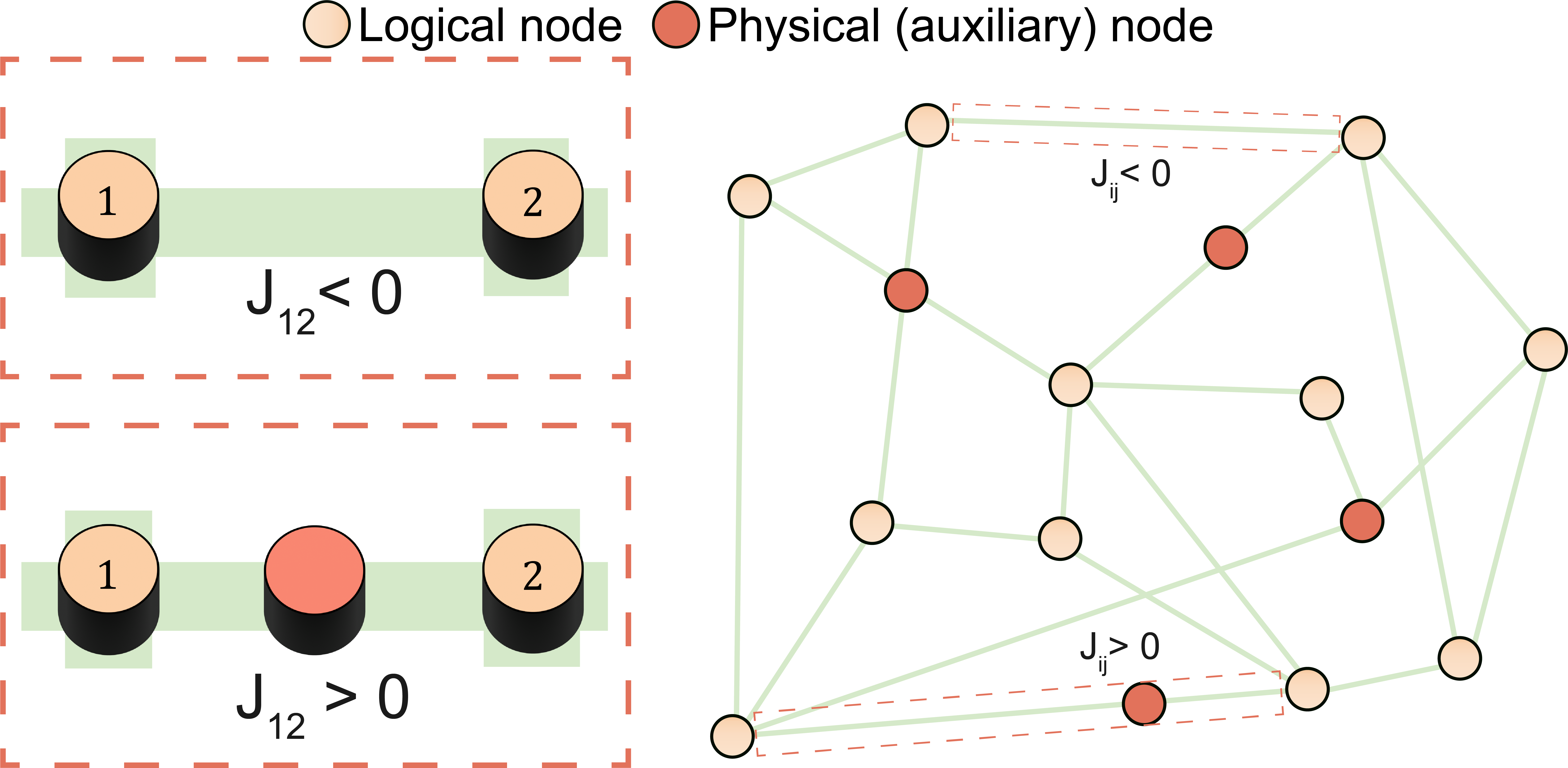
Figure S.3: Programming $\pm$ weights. Auxiliary magnets are introduced to choose the polarity of the interaction strength $J_{ij}$, where the input current is fixed such that all magnets have negative correlation ($J_{ij}<0$). The magnitude of the $J_{ij}$ is tuned by the channel length between any two spins ($\hat{m}_{i},\hat{m}_{j}$).

IX Physical parameters

Parameter	Value	Unit
Interface polarization ($P$)	0.1	–
Gilbert damping coefficient ($\alpha$)	0.01	–
Saturation magnetization ($M_{s}$)	1100 $\times 10^{3}$	A/m
Magnet volume ($\mathrm{Vol}.$)	(30 $\times$ 30 $\times$ 2)	nm3
Interface conductance ($G$)	1	S
Spin-Mixing conductance real part ($a\,G$)	1	–
Spin-Mixing Conductance Imaginary Part ($b\,G$)	0	–
NM Spin-Diffusion Length ($\lambda_{s}$)	400	nm
NM Resistivity ($\rho_{NM}$)	2.35	$\mu\Omega$.cm
NM Length ($L=L_{s}=L_{ch}$)	200	nm
NM Area ($A_{NM}$)	1.11 $\times 10^{-14}$	m2
Temperature	300	$K$
Transient Time Step (SPICE)	10	ps

The physical parameters we used in our simulations are reported in the Table above, where the parameters of the NM channel are chosen according to experiments performed in metallic non-local spin vales [31]. The transient noise (.trannoise) function of HSPICE has been used to solve the stochastic differential equations. This solver has been rigorously benchmarked with exact time-dependent Fokker-Planck equations in Ref. [27].

References

- Teh et al. [2003] Y. W. Teh, M. Welling, S. Osindero, and G. E. Hinton, Journal of Machine Learning Research 4, 1235 (2003).
- Berloff et al. [2017] N. G. Berloff, M. Silva, K. Kalinin, A. Askitopoulos, J. D. Töpfer, P. Cilibrizzi, W. Langbein, and P. G. Lagoudakis, Nature Materials 16, 1120 (2017).
- Huembeli et al. [2022] P. Huembeli, J. M. Arrazola, N. Killoran, M. Mohseni, and P. Wittek, Quantum Machine Intelligence 4, 10.1007/s42484-021-00057-7 (2022).
- Borders et al. [2019] W. A. Borders, A. Z. Pervaiz, S. Fukami, K. Y. Camsari, H. Ohno, and S. Datta, Nature 573, 390 (2019).
- Mohseni et al. [2022] N. Mohseni, P. L. McMahon, and T. Byrnes, Nature Reviews Physics 4, 363 (2022).
- Ramsauer et al. [2021] H. Ramsauer, B. Schäfl, J. Lehner, P. Seidl, M. Widrich, T. Adler, L. Gruber, M. Holzleitner, M. Pavlović, G. K. Sandve, V. Greiff, D. Kreil, M. Kopp, G. Klambauer, J. Brandstetter, and S. Hochreiter, Hopfield networks is all you need (2021), arXiv:2008.02217 .
- Ishihara et al. [2020] R. Ishihara, Y. Ando, S. Lee, R. Ohshima, M. Goto, S. Miwa, Y. Suzuki, H. Koike, and M. Shiraishi, Phys. Rev. Appl. 13, 044010 (2020).
- Panda et al. [2020] J. Panda, M. Ramu, O. Karis, T. Sarkar, and M. V. Kamalakar, ACS Nano 14, 12771 (2020).
- Bisswanger et al. [2022] T. Bisswanger, Z. Winter, A. Schmidt, F. Volmer, K. Watanabe, T. Taniguchi, C. Stampfer, and B. Beschoten, Nano Letters 22, 4949 (2022).
- Khokhriakov et al. [2022] D. Khokhriakov, S. Sayed, A. M. Hoque, B. Karpiak, B. Zhao, S. Datta, and S. P. Dash, Phys. Rev. Appl. 18, 064063 (2022).
- Camsari et al. [2017a] K. Y. Camsari, R. Faria, B. M. Sutton, and S. Datta, Physical Review X 7, 031014 (2017a).
- Camsari et al. [2017b] K. Y. Camsari, S. Salahuddin, and S. Datta, IEEE Electron Device Letters 38, 1767 (2017b).
- Kaiser et al. [2022] J. Kaiser, W. A. Borders, K. Y. Camsari, S. Fukami, H. Ohno, and S. Datta, Phys. Rev. Appl. 17, 014016 (2022).
- Grimaldi et al. [2022] A. Grimaldi, K. Selcuk, N. A. Aadit, K. Kobayashi, Q. Cao, S. Chowdhury, G. Finocchio, S. Kanai, H. Ohno, S. Fukami, and K. Y. Camsari, in 2022 International Electron Devices Meeting (IEDM) (2022) pp. 22.4.1–22.4.4.
- Hayakawa et al. [2021] K. Hayakawa, S. Kanai, T. Funatsu, J. Igarashi, B. Jinnai, W. A. Borders, H. Ohno, and S. Fukami, Phys. Rev. Lett. 126, 117202 (2021).
- Safranski et al. [2021] C. Safranski, J. Kaiser, P. Trouilloud, P. Hashemi, G. Hu, and J. Z. Sun, Nano Letters 21, 2040 (2021).
- Camsari et al. [2015] K. Y. Camsari, S. Ganguly, and S. Datta, Scientific Reports 5, 10.1038/srep10571 (2015).
- Sayed et al. [2016] S. Sayed, V. Q. Diep, K. Y. Camsari, and S. Datta, Scientific Reports 6, 10.1038/srep28868 (2016).
- Brataas et al. [2006] A. Brataas, G. E. Bauer, and P. J. Kelly, Physics Reports 427, 157 (2006).
- Srinivasan et al. [2016] S. Srinivasan, V. Diep, B. Behin-Aein, A. Sarkar, and S. Datta, Modeling multi-magnet networks interacting via spin currents, in Handbook of Spintronics, edited by Y. Xu, D. Awschalom, and J. Nitta (Springer Netherlands, 2016) pp. 1281–1335.
- Manipatruni et al. [2012] S. Manipatruni, D. E. Nikonov, and I. A. Young, IEEE Transactions on Circuits and Systems I: Regular Papers 59, 2801 (2012).
- Brown Jr [1963] W. F. Brown Jr, Physical review 130, 1677 (1963).
- Sun [2000] J. Z. Sun, Physical Review B 62, 570 (2000).
- Sun et al. [2004] J. Z. Sun, T. Kuan, J. Katine, and R. H. Koch, in Quantum Sensing and Nanophotonic Devices, Vol. 5359 (SPIE, 2004) pp. 445–455.
- Butler et al. [2012] W. H. Butler, T. Mewes, C. K. A. Mewes, P. B. Visscher, W. H. Rippard, S. E. Russek, and R. Heindl, IEEE Transactions on Magnetics 48, 4684 (2012).
- Kimura et al. [2006] T. Kimura, Y. Otani, and J. Hamrle, Physical review letters 96, 037201 (2006).
- Torunbalci et al. [2018] M. M. Torunbalci, P. Upadhyaya, S. A. Bhave, and K. Y. Camsari, IEEE Transactions on Electron Devices 65, 4628 (2018).
- Datta et al. [2011] D. Datta, B. Behin-Aein, S. Datta, and S. Salahuddin, IEEE Transactions on Nanotechnology 11, 261 (2011).
- Kobayashi et al. [2023] K. Kobayashi, N. Singh, Q. Cao, K. Selcuk, T. Hu, S. Niazi, N. A. Aadit, S. Kanai, H. Ohno, S. Fukami, et al., arXiv preprint arXiv:2304.05949 (2023).
- Debashis et al. [2022] P. Debashis, H. Li, D. Nikonov, and I. Young, IEEE Magnetics Letters 13, 1 (2022).
- Kimura et al. [2008] T. Kimura, T. Sato, and Y. Otani, Phys. Rev. Lett. 100, 066602 (2008).
- Hinton et al. [1984] G. E. Hinton, T. J. Sejnowski, and D. H. Ackley, Boltzmann Machines: Constraint Satisfaction Networks That Learn, Tech. Rep. CMU-CS-84-119, (Computer Science Department, Carnegie Mellon University, 1984).
- Ackley et al. [1985] D. H. Ackley, G. E. Hinton, and T. J. Sejnowski, Cognitive Science 9, 147 (1985).
- Hong et al. [2012] S. Hong, V. Diep, S. Datta, and Y. P. Chen, Physical Review B 86, 085131 (2012).
- Kim et al. [2019] J. Kim, C. Jang, X. Wang, J. Paglione, S. Hong, J. Lee, H. Choi, and D. Kim, Physical Review B 99, 245148 (2019).
- Choi et al. [2022] W. Y. Choi, I. C. Arango, V. T. Pham, D. C. Vaz, H. Yang, I. Groen, C.-C. Lin, E. S. Kabir, K. Oguz, P. Debashis, et al., Nano Letters 22, 7992 (2022).
- Pham et al. [2020] V. T. Pham, I. Groen, S. Manipatruni, W. Y. Choi, D. E. Nikonov, E. Sagasta, C.-C. Lin, T. A. Gosavi, A. Marty, L. E. Hueso, et al., Nature Electronics 3, 309 (2020).
- Liu et al. [2012] L. Liu, C.-F. Pai, Y. Li, H. Tseng, D. Ralph, and R. Buhrman, Science 336, 555 (2012).
- Behin-Aein et al. [2010] B. Behin-Aein, D. Datta, S. Salahuddin, and S. Datta, Nature nanotechnology 5, 266 (2010).
- Alaghi and Hayes [2013] A. Alaghi and J. P. Hayes, ACM Transactions on Embedded computing systems (TECS) 12, 1 (2013).
- Harabi et al. [2022] K.-E. Harabi, T. Hirtzlin, C. Turck, E. Vianello, R. Laurent, J. Droulez, P. Bessière, J.-M. Portal, M. Bocquet, and D. Querlioz, Nature Electronics 10.1038/s41928-022-00886-9 (2022).
- Debashis et al. [2020] P. Debashis, V. Ostwal, R. Faria, S. Datta, J. Appenzeller, and Z. Chen, Scientific Reports 10, 10.1038/s41598-020-72842-6 (2020).
- Bunaiyan and Camsari [2023] S. Bunaiyan and K. Y. Camsari, Heisenberg machines (HSPICE code), https://github.com/OPUSLab/HeisenbergMachines (2023).