Diffusion Posterior Sampling for Nonlinear CT Reconstruction

Abstract

Diffusion models have been demonstrated as powerful deep learning tools for image generation in CT reconstruction and restoration. Recently, diffusion posterior sampling, where a score-based diffusion prior is combined with a likelihood model, has been used to produce high quality CT images given low-quality measurements. This technique is attractive since it permits a one-time, unsupervised training of a CT prior; which can then be incorporated with an arbitrary data model. However, current methods only rely on a linear model of x-ray CT physics to reconstruct or restore images. While it is common to linearize the transmission tomography reconstruction problem, this is an approximation to the true and inherently nonlinear forward model. We propose a new method that solves the inverse problem of nonlinear CT image reconstruction via diffusion posterior sampling. We implement a traditional unconditional diffusion model by training a prior score function estimator, and apply Bayes rule to combine this prior with a measurement likelihood score function derived from the nonlinear physical model to arrive at a posterior score function that can be used to sample the reverse-time diffusion process. This plug-and-play method allows incorporation of a diffusion-based prior with generalized nonlinear CT image reconstruction into multiple CT system designs with different forward models, without the need for any additional training. We develop the algorithm that performs this reconstruction, including an ordered-subsets variant for accelerated processing and demonstrate the technique in both fully sampled low dose data and sparse-view geometries using a single unsupervised training of the prior.

1 INTRODUCTION

Neural networks have been widely investigated for CT reconstruction and have shown impressive performance capabilities [1, 2, 3]. Recently, diffusion models have been shown to be particularly powerful deep learning tools for CT reconstruction and restoration [4, 5, 6, 7, 8]. Such methods have generally been based on denoising diffusion probabilistic models (DDPM) [9] and score-based generative diffusion models through stochastic differential equations (SDEs) [10]. Most diffusion models for CT reconstruction have been trained in a supervised manner, where the conditional data input is known in both training and generation [7, 8, 11]. Recent research on image denoising and restoration has demonstrated the potential of unsupervised training by leveraging the power of posterior sampling, where the conditional data input is only available during the reverse-time diffusion process [12, 13, 5]. The unsupervised training does not assume a fixed measurement process during training, and can thus be flexibly incorporated with different measurement models without retraining. In these efforts, the measurement model has been presumed to be linear. Lopez-Montes et al.[14] have recently applied such an approach using a linearized model to tomographic data.

It is well-known that the transmission tomography forward model that relates the underlying attenuation values to the measurements is nonlinear. While the model is commonly linearized for mathematical convenience, such approximation can result in deviation from the true underlying data model and can cause problems in many circumstances including models for very low dose data [15], beam-hardening [16], and detector blur [17]. In this work, we propose an approach for nonlinear CT image reduction using diffusion posterior sampling (which we will refer to as DPS Nonlinear). Specifically, we seek to solve the inverse problem of CT image reconstruction via DPS with a score-based diffusion prior and a physics-driven measurement likelihood term. This method guides the updates of the reverse-time diffusion process so that the final results are consistent with the raw (nonlinear) measurements from a CT imaging system. Our approach trains a traditional score-based diffusion model for unconditional CT image generation and applies Bayes rule by adding the gradient of the log-likelihood (i.e.) from the non-linear physical model to achieve the posterior score function necessary for DPS. The method is plug-and-play, meaning it does not require any extra training for application to a different CT system measurement model.

2 METHODS

2.1 Diffusion Posterior Sampling using a Nonlinear Physical Model

The proposed DPS Nonlinear method combines diffusion posterior sampling with a nonlinear physical model. This approach requires estimation of the prior distribution of CT images using a score-based generative model [9, 10]. Specifically, a diffusion model is adopted wherein a forward stochastic process is defined where an image is perturbed by successively added noise. A reverse process is then defined where we may sample images from the estimated prior distribution starting from a noise image. Specifically, we follow prior work [9, 10] where the forward diffusion process is governed by

$$\mathbf{x_{t}}=\sqrt{\bar{\alpha}_{t}}\mathbf{x_{0}}+(1-\bar{\alpha}_{t})\mathbf{\epsilon_{noise}}\;\;\;t\in(0,T],$$ (1)

where $\mathbf{\epsilon_{noise}}\sim N(0,I)$ is Gaussian noise, $\mathbf{x_{0}}\sim\mathbf{p_{data}}$ denote a true image sampled from a training dataset, $\bar{\alpha}_{t}$ is a variance scheduler such that the final noise is close to a predefined noise distribution $\mathbf{\pi(x)}$, and the process is defined on $t\in(0,T]$. The final sample $\mathbf{p_{t=T}}$ usually follows the predefined noise distribution $\mathbf{\pi(x)}$ and it does not contain any information of training dataset $\mathbf{p_{data}}$ or $\mathbf{p_{t=0}}$. To recover the data in a tractable distribution, which can be achieved by reversing the perturbation forward process in Equation (1) to get the reverse-time SDE given by

$$\mathbf{dx_{t}}=[\mathbf{f}(\mathbf{x_{t}},t)+g^{2}(t)\nabla_{\mathbf{x_{t}}}\log p(\mathbf{x_{t}})]dt+g(t)\mathbf{d\bar{w}_{t}}\;\;\;t\in(0,T],$$ (2)

where $\mathbf{f}$ is drift coefficient term for $\mathbf{x_{t}}$ defined by $\mathbf{f}(\mathbf{x_{t}},t)=-1/2\beta_{t}\mathbf{x_{t}}$, $g$ is the diffusion coefficient for $\mathbf{x_{t}}$ defined by $g(t)=\sqrt{\beta_{t}}$, $\beta_{t}=-1/\sqrt{\bar{\alpha}_{t}}\frac{d}{dt}\bar{\alpha}_{t}$, $\bar{\mathbf{w}}$ is a standard Wiener process when reverse-time flows from T to 0, and $dt$ is an infinitesimal negative timestep. The continuous structure also allows for the production of data samples from $\mathbf{p_{0}}(\mathbf{x_{0}}|\mathbf{y})$ if the posterior $\mathbf{y}$ and $\mathbf{p_{t}}(\mathbf{y}|\mathbf{x_{t}})$ is known. Equation (2) then can be transformed into a conditional reverse-time SDE:

$$\mathbf{dx_{t}}=[\mathbf{f}(\mathbf{x_{t}},t)+g^{2}(t)\nabla_{\mathbf{x_{t}}}\log p(\mathbf{x_{t}}|\mathbf{y})]dt+g(t)\mathbf{d\bar{w}_{t}}\;\;\;t\in(0,T].$$ (3)

Furthermore, applying the Bayes rule, the conditioned reverse stochastic process in Equation (3) for diffusion posterior sampling is given by

$$\mathbf{d\mathbf{x_{t}}}=[\mathbf{f}(\mathbf{x_{t}},t)+g^{2}(t)(\nabla_{\mathbf{x_{t}}}\log p(\mathbf{x_{t}})+\nabla_{\mathbf{x_{t}}}\log p(\mathbf{y}|\mathbf{x_{t}}))]dt+g(t)\mathbf{d\bar{w}_{t}}\;\;\;t\in(0,T].$$ (4)

Following previous score matching methods[10, 18], the prior score $\nabla_{\mathbf{x_{t}}}\log p(\mathbf{x_{t}})$ is estimated by a neural network to form a score model $\mathbf{s_{\theta}}(\mathbf{x_{t}},t)$ using the following loss function:

$$\theta^{*}=\arg\min_{\theta}\ E_{t\sim u(\epsilon,1),\mathbf{x_{t}}\sim p(\mathbf{x_{t}}|\mathbf{x_{0}}),\mathbf{x_{0}}\sim\mathbf{p_{data}}}[||\mathbf{s_{\theta}}(\mathbf{x_{t}},t)-\nabla_{\mathbf{x_{t}}}\log p(\mathbf{x_{t}}|\mathbf{x_{0}})||^{2}_{2}],$$ (5)

where network parameters, $\theta$, are estimated through a training process and the expected loss is evaluated over the uniform distribution timestep $t\in(0,T]$ and degraded images $\mathbf{x_{t}}$. The degraded images are generated by perturbing ground truth images $\mathbf{x_{0}}$ from a training dataset for the corresponding timestep $t$. Plugging the score estimate into Equation (4) yields the resulting reverse-time SDE:

$$\mathbf{dx_{t}}=[\mathbf{f}(\mathbf{x_{t}},t)+g^{2}(t)(\mathbf{s_{\theta^{*}}}(\mathbf{x_{t}},t)+\nabla_{\mathbf{x_{t}}}\log p(\mathbf{y}|\mathbf{x_{t}}))]dt+g(t)\mathbf{d\bar{w}_{t}}\;\;\;t\in(0,T].$$ (6)

Following Chung et al.[13], the gradient of the likelihood term, $\nabla_{\mathbf{x_{t}}}\log p(\mathbf{y}|\mathbf{x_{t}})$, can be approximated as follows

$$\nabla_{\mathbf{x_{t}}}\log p(\mathbf{y}|\mathbf{x_{t}})=\nabla_{\mathbf{x_{t}}}\mathbf{\hat{x}_{0}}(\mathbf{x_{t}})\nabla_{\mathbf{x_{0}}}\log p(\mathbf{y}|\mathbf{x_{0}}=\mathbf{\mathbf{\hat{x}_{0}}})\;\;\;\text{where}\;\;\;\mathbf{\hat{x}_{0}}=\frac{1}{\sqrt{\bar{\alpha}_{t}}}(\mathbf{x_{t}}+(1-\bar{\alpha}_{t})\mathbf{s_{\theta^{*}}}(\mathbf{x_{t}},t)),$$ (7)

where $\mathbf{\hat{x}_{0}}$ denotes an approximation of $\mathbf{x_{0}}$ from $\mathbf{x_{t}}$, and $\nabla_{\mathbf{x_{t}}}$ denotes the gradient with respect to $\mathbf{x_{t}}$. For $\nabla_{\mathbf{x_{0}}}\log p(\mathbf{y}|\mathbf{x_{0}}=\mathbf{\hat{x}_{0}})$, we propose to apply a nonlinear physical model defined by a Gaussian distribution:

$$\mathbf{y}\sim N(\mathbf{\bar{y}},\mathbf{D}\{\mathbf{y}\})\;\;\;\text{where}\;\;\;\mathbf{\bar{y}}(\mathbf{x_{0}})=\mathbf{B}\exp(-\mathbf{A}\mathbf{x_{0}}),$$ (8)

where $\mathbf{\bar{\mathbf{y}}}$ denotes the mean measurement vector, $\mathbf{y}$ denotes the real projection coming from different CT system, $\mathbf{x_{0}}$ denotes the image of attenuation coefficients in transmission tomography, $\mathbf{A}$ is the linear projection matrix defined for a given CT imaging system, $\mathbf{D\{\cdot\}}$ represent a diagonal matrix. $\mathbf{B}$ is a matrix operator that can model various physical effects including measurement-dependent fluence levels, detector blur, etc. as in Tilley et al. [19] Given independent Gaussian noise with measurement variance $\mathbf{\sigma_{y}}=\mathbf{y}$ (approximating Poisson noise), one may write the measurement log-likelihood as

$$\log p(\mathbf{y}|\mathbf{{x}_{0}})=-\frac{1}{2}(\mathbf{y}-\bar{\mathbf{y}}(\mathbf{{x}_{0}}))^{T}\mathbf{D}^{-1}\{\mathbf{y}\}(\mathbf{y}-\bar{\mathbf{y}}(\mathbf{{x}_{0}})),$$ (9)

which includes the explicit dependence of the mean measurement model, $\bar{\mathbf{y}}$, on the underlying true image, $\mathbf{x_{0}}$, as defined in (8). Applying the chain rule, the gradient of this equation with respect to $\mathbf{x_{0}}$ is

$$\nabla_{\mathbf{{x}_{0}}}\log p(\mathbf{y}|\mathbf{{x}_{0}})=\bar{\mathbf{y}}^{\prime}(\mathbf{{x}_{0}})^{T}\mathbf{D}^{-1}\{\mathbf{y}\}(\mathbf{y}-\bar{\mathbf{y}}(\mathbf{{x}_{0}})))$$ (10)

where

$$\bar{\mathbf{y}}^{\prime}(\mathbf{{x}_{0}})=-\mathbf{A}^{T}\mathbf{D}\{\exp(-\mathbf{A}\mathbf{{x}_{0}})\}\mathbf{B}^{T}.$$ (11)

Combining terms and plugging in for the mean measurement model, we may write the expression

$$\nabla_{\mathbf{x_{0}}}\log p(\mathbf{y}|\mathbf{x_{0}})=-\mathbf{A}^{\text{T}}\mathbf{D}\{\exp(-\mathbf{A}\mathbf{x_{0}})\}\mathbf{B}^{\text{T}}\mathbf{D}\{1/\mathbf{y}\}(\mathbf{y}-\mathbf{B}\exp(-\mathbf{A}\mathbf{x_{0}})),$$ (12)

where $\{\cdot\}^{\text{T}}$ denotes a matrix transpose with $\mathbf{A}^{\text{T}}$ representing backprojection. Equations (7) and (12) are plugged into Equation (4) to enable nonlinear physical model based diffusion posterior sampling in a reverse-time diffusion process.

2.2 Unconditional Training in Forward Diffusion

A neural network is used to estimate the score function in the unconditional score-based diffusion model [10]. This network may be trained in an unsupervised fashion independent of the measurement model. The resulting DPS Nonlinear method does not require any extra training for different CT systems. In this work, we adopt a U-Net [20] with an attention residual module and time embedding module[10] for score estimation. The XCAT phantom[21] was used for the dataset of prior score model training. A total of 54 human models were divided into training, validation, and test sets with a ratio of approximately 8:1:1 and then individual slices of 256 $\times$ 256 voxels were extracted for each dataset. Individual human models were divided across datasets to avoid mixing between training, validation, and testing. For the stochastic process, we adopted a schedule defined by $\bar{\alpha}_{t}=1e^{-5t}$ with $t\in(0,T]$ where $T=1$. For training, we applied Adam optimizer, setting the batch size to 8 and the initial learning rate to 0.001. We trained our score estimator over 600 Epochs with early stopping to get the best weights for the prior score function. This trained score model was subsequently used for CT reconstruction for different CT system models.

2.3 Reconstruction using Diffusion Posterior Sampling

For the reverse-time diffusion, we plug in the likelihood score function and generate the samples with the prior score function from the trained score model. The algorithm includes a time-dependent coefficient scheduler $\lambda(t)$, which balances the weighting between the likelihood score function and the prior score function over the process of reverse-time diffusion. Following Chung et al. [13], taking the derivative of the prior score function $\mathbf{s_{\theta^{*}}}(\mathbf{x_{t}},t)$ with respect to the input $\mathbf{x_{t}}$ is accomplished by calculating the Jacobian matrix using backward propagation in the score model. We adopted the standard Variance Preserving Stochastic Stochastic Differential Equations (VP-SDEs) to discretize the reverse process into $N$ bins. The final DPS Nonlinear reconstruction algorithm is summarized in Algorithm 1.

$\mathbf{x_{1}}\sim N(0,I)$,  $\mathbf{\hat{y}}\leftarrow I_{0}\exp(-\mathbf{A}\mathbf{x_{y}})$,  $\mathbf{y}\sim N(\mathbf{\hat{y}},\mathbf{\hat{y}})$,  $\lambda(t)$, $\Delta t\leftarrow\frac{1}{N}$;

for $i=N-1\ \text{to}\ 0$ do

        $t\leftarrow(i+1)/N$

       $\mathbf{\hat{s}}\leftarrow\mathbf{s_{\theta}^{*}}(\mathbf{x_{t}},t)$

       $\mathbf{\hat{x}_{0}}\leftarrow\frac{1}{\sqrt{\bar{\alpha}_{t}}}(\mathbf{x_{t}}+(1-\bar{\alpha}_{t})\mathbf{\hat{s}})$

       $\mathbf{\Delta_{x_{t}}}\leftarrow-\mathbf{A^{T}}\exp(-\mathbf{A}\mathbf{\hat{x}_{0}}){\mathbf{y^{-1}}}I_{0}(\mathbf{y}-I_{0}\exp(-\mathbf{A}\mathbf{\hat{x}_{0}}))$

       $\mathbf{\Delta_{x_{0}}}\leftarrow\frac{1}{\sqrt{\bar{\alpha}_{t}}}(1+(1-\bar{\alpha}_{i})\nabla_{\mathbf{x_{t}}}\mathbf{\hat{s}}(\mathbf{x_{t}}))\;\;\;\#\nabla_{\mathbf{x_{t}}}\mathbf{\hat{s}}(\mathbf{x_{t}})\;is\;taking\;the\;backpropagation_{\theta^{*}}(\mathbf{\hat{s}})\>w.r.t\>\mathbf{x_{t}}$

       $\mathbf{dx}\leftarrow[\mathbf{f}(t)\mathbf{x_{t}}+g^{2}(t)(\mathbf{\hat{s}}+\lambda(t)\mathbf{\Delta_{x_{0}}}\mathbf{\Delta_{x_{t}}})]dt$

       $\mathbf{z}\sim N(0,I)$

       $\mathbf{x_{t-\Delta t}}\leftarrow\mathbf{x_{t}}-\mathbf{dx}+g(t)\sqrt{\Delta t}\mathbf{z}$

end for

Algorithm 1 DPS Nonlinear

The probabilistic framework of the DPS model allows a separation of the prior model and the measurement model. This separation is explicit both mathematically in the application of Bayes rule, but also in the resulting algorithm which alternates between reverse diffusion updates and gradient-based updates based on the likelihood model. Thus, the DPS approach can be viewed as a way to merge model-based iterative reconstruction (MBIR) and a diffusion-based prior. Indeed, if the diffusion prior were removed, one would have a maximum-likelihood approach that uses a gradient ascent algorithm for iterations. This also suggests that one may leverage some of the many acceleration strategies that have been applied in MBIR to improve the efficiency of DPS. This was also recognized by Wenjun et al [22]. Here, we modify the DPS Nonlinear approach to use ordered-subsets.[23, 24, 25]

In short, in classic MBIR, it was found that the gradient of the likelihood can be well-approximated by a subset of the projection data (usually a fraction of projection angles from regularly spaced data), which requires only a fraction of the computations associated with the full projection ($\mathbf{A}$) or backprojection ($\mathbf{A}^{T}$). To apply the same technique to DPS Nonlinear, we divide the projections into assigned number of subsets $N_{os}$. Instead of using the whole projection $\mathbf{y}$, updates are based on rotating subsets of projections, applied in turn $\mathbf{y_{j}}$ where $j\in\;\{1,2,3,...,N_{os}\}$. One can interpret this with as Order-Subset nonlinear diffusion posterior sampling (OS-DPS Nonlinear), given by

$$\mathbf{d}\mathbf{x_{t}}=[\mathbf{f}(\mathbf{x_{t}},t)+g^{2}(t)(\nabla_{\mathbf{x_{t}}}\log p(\mathbf{x_{t}})+\nabla_{\mathbf{x_{t}}}\log p_{j}(\mathbf{y_{j}}|\mathbf{x_{t}})]dt+g(t)\mathbf{d}\mathbf{\bar{w}_{t}}\;\;\;t\in(0,T]\;\;\;j\in\{1,2,3,...,N_{os}\},$$ (13)

where $j$ is the current index of subset. The subset $j$ can be calculated by $mod(i,N_{os})$, which is taking the remainder of current index of iteration $i$ divided by number of total order subsets. The likelihood term for each order subset $\nabla_{\mathbf{x_{t}}}\log p_{j}(\mathbf{y_{j}}|\mathbf{x_{t}})$ is updated through the following equation

$$\nabla_{\mathbf{x_{0}}}\log p_{j}(\mathbf{y_{j}}|\mathbf{x_{0}})=-\mathbf{A_{j}}^{\text{T}}D\{\exp(-\mathbf{A_{j}}\mathbf{x_{0}})\}\mathbf{B}^{\text{T}}D\{1/\mathbf{y_{j}}\}(\mathbf{y_{j}}-\mathbf{B}\exp(-\mathbf{A_{j}}\mathbf{x_{0}}))\;\;\;j\in\{1,2,3,...,N_{os}\},$$ (14)

where $\mathbf{A_{j}}$ denotes subset projection matrices, and $\mathbf{A^{T}_{j}}$ are the associated subset backprojection matrices. The DPS Nonlinear method can be treated as a special case of OS-DPS Nonlinear when the $N_{os}=1$. The OS-DPS Nonlinear algorithm is summarized in Algorithm 2.

$\mathbf{x_{1}}\sim N(0,I)$,  $\mathbf{\hat{y}_{j}}\leftarrow I_{0}\exp(-\mathbf{A_{j}}\mathbf{x_{y}})$, $\mathbf{y_{j}}\sim N(\mathbf{\hat{y}_{j}},\mathbf{\hat{y}_{j}})$,  $\Delta t\leftarrow\frac{1}{N}$, $\lambda(t)$, $j\in\{1,2,3,...,N_{os}\}$;

for $i=N-1\ \text{to}\ 0$ do

        $t\leftarrow(i+1)/N$

       $j\leftarrow mod(i+1,N_{os})$

       $\mathbf{\hat{s}}\leftarrow\mathbf{s_{\theta}^{*}}(\mathbf{x_{t}},t)$

       $\mathbf{\hat{x}_{0}}\leftarrow\frac{1}{\sqrt{\bar{\alpha}_{t}}}(\mathbf{x_{t}}+(1-\bar{\alpha}_{t})\mathbf{\hat{s}})$

       $\mathbf{\Delta_{x_{t}}}\leftarrow-\mathbf{A_{j}^{T}}\exp(-\mathbf{A_{j}}\mathbf{\hat{x}_{0}})\mathbf{y_{j}^{-1}}I_{0}(\mathbf{y_{j}}-I_{0}\exp(-\mathbf{A_{j}}\mathbf{\hat{x}_{0}}))$

       $\mathbf{\Delta_{x_{0}}}\leftarrow\frac{1}{\sqrt{\bar{\alpha}_{t}}}(1+(1-\bar{\alpha}_{i})\nabla_{\mathbf{x_{t}}}\mathbf{\hat{s}}(\mathbf{x_{t}}))\;\;\;\#\nabla_{\mathbf{x_{t}}}\mathbf{\hat{s}}(\mathbf{x_{t}})\;is\;taking\;the\;backpropagation_{\theta^{*}}(\mathbf{\hat{s}})\>w.r.t\>\mathbf{x_{t}}$

       $\mathbf{dx}\leftarrow[\mathbf{f}(t)\mathbf{x_{t}}+g^{2}(t)(\mathbf{\hat{s}}+\lambda(t)\mathbf{\Delta_{x_{0}}}\mathbf{\Delta_{x_{t}}}]dt$

       $\mathbf{z}\sim N(0,I)$

       $\mathbf{x_{t-\Delta t}}\leftarrow\mathbf{x_{t}}-\mathbf{dx}+g(t)\sqrt{\Delta t}\mathbf{z}$

end for

Algorithm 2 OS-DPS Nonlinear

2.4 Evaluation of DPS Nonlinear and OS-DPS Nonlinear

We evaluate DPS Nonlinear in two different scenarios: 1) Fully sampled low-dose CT reconstruction; and 2) Sparse-view CT reconstruction. For comparison, we compute standard filtered-backprojection (FBP) and model-based iterative reconstructions (MBIR). For the model-based iterative reconstructions, we apply our nonlinear physical model to maximum-likelihood reconstruction using gradient ascent with a fixed step size. For each approach we report Peak Signal-to-Noise ratio (PSNR) and Structured Similarity (SSIM). Additionally, we evaluate OS-DPS Nonlinear in the fully sampled low-dose CT reconstruction scenario and in a limited computation case. For all the experiments, we emulate a system geometry with a source-to-detector distance of 1500 mm, and a source-to-axis distance of 1000 mm. We choose the simple case of $\mathbf{B}=I_{0}$, where $I_{0}$ is a scalar defining the mean number of photons/detector pixel in barebeam. Projections are one-dimensional with 1024 - 0.8 mm pixels. All the systems are implemented using LEAP projectors/backprojectors[26] and PyTorch. Detailed settings and parameters are defined in the following experiments.

2.4.1 Low-dose CT Reconstruction Comparisons

For the low-dose CT reconstruction scenario, $I_{0}=10^{3}$ photons/pixel with 360 projections covering $360^{\circ}$. The lambda scheduler was set to $\lambda(t)=10^{-3.1t-0.7}$ where the $t$ is the reverse timestep from 1 to 0. The number of iterations in the reverse-diffusion is set to $1000$. For the MBIR, we adopt $40000$ gradient ascent iterations with step size equals to $6\times 10^{-7}$.

2.4.2 Sparse view CT reconstruction Comparisons

Sparse view CT reconstruction is applied to a system with $I_{0}=10^{5}$ photons/pixel with 30 projects cover $360^{\circ}$. In this case, the lambda scheduler is set to $\lambda(t)=10^{-4.3t-1.5}$ and the number of iterations in the reverse diffusion process is set to $1000$. For MBIR, we adopt $150000$ gradient ascent iterations with step size equals to $3\times 10^{-8}$.

2.4.3 OS-DPS Nonlinear Comparisons

For evaluation of OS-DPS Nonlinear, use the same scenario as low-dose CT reconstruction. The system is defined by $I_{0}=10^{3}$ photons/pixel with 360 projections covering $360^{\circ}$. We consider 1, 6, 12, 24, 36, 48, and 60 ordered subsets (OS) for the comparison. The lambda scheduler remains the same as the low-dose CT reconstruction when the OS = 1 and is modified to $10^{-5.5t+1.7}$ for OS = 6, $10^{-6.6t+2.8}$ for OS = 12, $10^{-7.5t+3.7}$ for OS = 24, $10^{-8.4t+4.6}$ for OS = 36, $10^{-8.8t+4}$ for OS = 48, and $10^{-9.2t+5.4}$ for OS = 60. According to the Equation (6), $\lambda(t)$ should not be greater than 1 during the whole reverse-time process. Therefore, any lambda in the reverse process that is greater than 1 is thresholded back to 1. We first apply the same $1000$ iterations in the reverse-diffusion to evaluate differences. In addition to PSNR and SSIM, we proposed another way of comparing the results generated by diffusion posterior sampling. For a single input image, we run the posterior sampling to generate 32 results. Based on these 32 generated results, we take the mean and standard deviation of them to get the sample mean image and standard deviation image. We further subtract the mean from the ground truth image to get a bias image. We compare sample mean image, bias image, and standard deviation images between different numbers of ordered subsets.

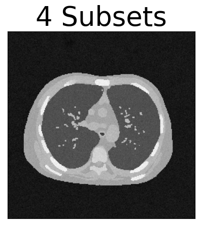
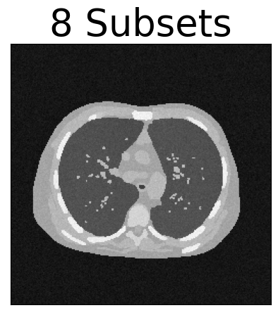
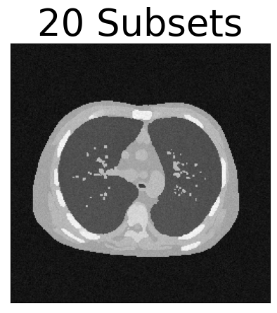
To further test our method, we apply our OS-DPS Nonlinear under a different scenario where the system is defined by $I_{0}=10^{4}$ photons/pixel with $200$ projections over $360^{\circ}$. To consider the potential of ordered subsets under limited computation time, we compare results with a relatively low fixed number of $200$ iterations/time steps. The lambda scheduler is set to $10^{-3.4t-1.4}$ for OS = 4, $10^{-3.7t+1.1}$ for OS = 8, and $10^{-4.1t-0.7}$ for OS = 20.

3 Results

3.1 Low-dose CT Reconstruction

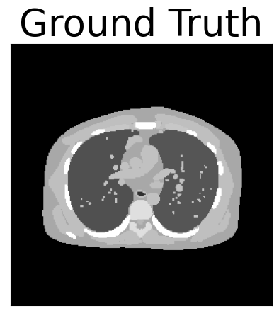
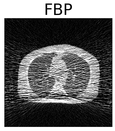
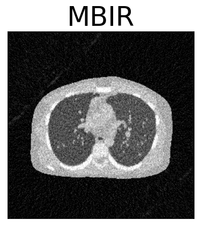
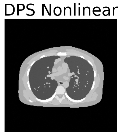
Figure 1 shows reconstructions in the low-dose CT scenario. We see that the proposed DPS reconstruction yields a sharp image with recognizable anatomical structures, indicating that the proposed method is capable of guiding the unconditional diffusion generation through the posterior sampling. In contrast, the FBP reconstruction has heavy streaking associated with the very low x-ray fluence (particularly along the long axis and the spine where photon starvation effects are more pronounced.) The MBIR approach is both noisy and with residual blur, obscuring many fine details. We found the PSNR of FBP was $27.67$ dB, MBIR was $32.26$ dB, and the DPS approach was $54.55$ dB. For the SSIM, DPS achieved $0.7224$ while FBP was $0.0742$ and MBIR was $0.2082$. These quantitative measures exhibit the same rank ordering of our subjective image quality assessment.

Figure 1: Low-dose CT reconstructions comparing FBP, MBIR, and the proposed DPS Nonlinear approach. All images share a common colormap with W/L = 2000/0 HU.

Looking closely at the DPS reconstruction for low-dose CT reconstruction, we note that the generative aspect of the DPS approach is evident. There are features in the DPS reconstruction that do not match exactly those found in the ground truth. Such hallucinations are common with these generative approaches - particularly when applied to very low-fidelity data as in this scenario.

Figure 2: Additional DPS sample reconstructions from the same data illustrating variability in the outputs.

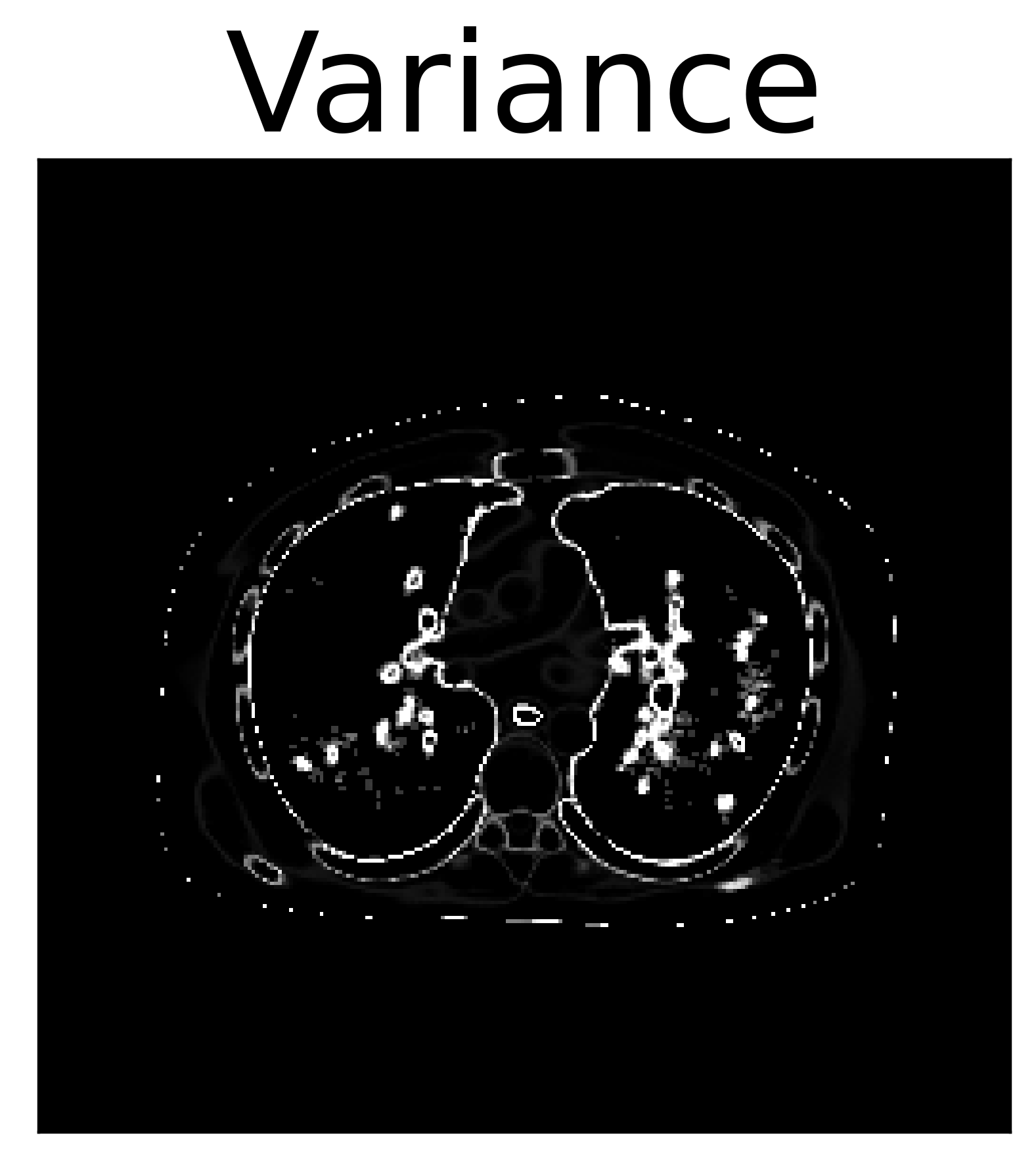
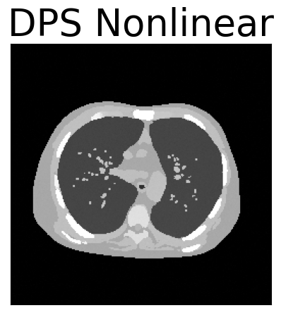
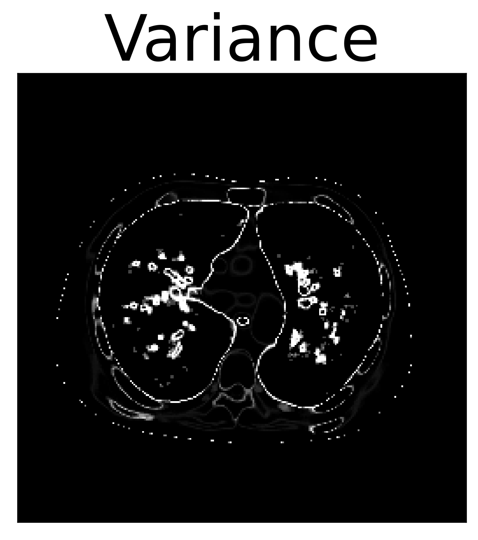
Figure 2 further explores some of the generative aspects of the proposed DPS approach. Among several sample outputs applied to the same data, one can see both common features and variable features in the reconstruction. In general, DPS Nonlinear is more stable in the generation of low frequency general structures than the high frequency details. In particular, the fine details in the lung tend to be most variable with more consistency in major high contrast structures. This is particularly evident from a variance image computed from 32 of these DPS examples. Note the increased variability at tissue boundaries and in the smaller features in the lungs.

3.2 Sparse-view CT Reconstruction

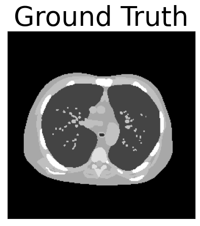
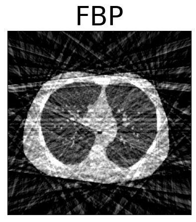
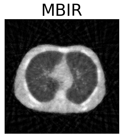
Figure 3 illustrates the flexibility of the DPS Nonlinear approach with application to a sparse-view CT reconstruction. Again, we see that the DPS Nonlinear approach yields an image with sharp edges and recognizable features. In this case, there is better agreement with the underlying ground truth (suggesting, perhaps, less reliance on the generative nature of DPS and a better conditioned reconstruction problem). The FBP reconstruction exhibits obvious streaking due to undersampling, and MBIR shows significant blur and noise. In terms of PSNR, our proposed method DPS Nonlinear yielded $59.54$ dB versus $27.66$ dB with FBP and $37.15$ dB with MBIR. For SSIM, our method achieved $0.6774$ while FBP and MBIR was $0.2392$ and $0.3093$, respectively. Again, these quantitative measures agree well with perceived image quality.

Figure 3: Sparse-view CT reconstructions comparing, FBP, MBIR, and DPS Nonlinear. Colormap: W/L = 2000/0 HU.

As in the low-dose situation, we generated 32 samples and computed a variance image. Three DPS Nonlinear reconstructions are shown to illustrate some of the variability associated with the stochastic reverse process. Three examples and the variance image are shown in Figure 4. Similar to the low-dose scenario, DPS Nonlinear tends to be more stable in the generation of low frequency general structures than the high frequency details in the lung and at tissue boundaries.

Figure 4: Additional DPS sample reconstructions from the same data illustrating variability in the outputs.

3.3 OS-DPS Nonlinear Evaluations

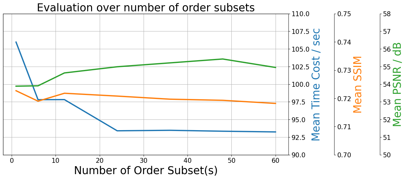
Figure 5 illustrates the mean computation time, SSIM, and PSNR of 32 samples for OS-DPS Nonlinear with different numbers of ordered subsets. Note that the computation time reached a plateau when the OS = 24 at around 93 seconds with a peak at OS=1 at 106 seconds. This represents a speed-up of around $12\%$. Recall that the ordered subsets approach is only speeding up the construction of likelihood term in Equation (6), indicating that the reverse diffusion update in the DPS Nonlinear reverse process remain a significant contributor to overall computation time. We did not observe a significant drop on the SSIM and PSNR as the number of subsets increased. The mean SSIM went up $\sim 2\%$ and mean PSNR went down only $\sim 0.5\%$.

Figure 5: The mean computation time, SSIM, and PSNR over the 32 samples generated under different number of order subsets with $1000$ iterations. The mean time cost represents the time OS-DPS Nonlinear takes to generate one sample.

Figure 6: Comparison of sample mean image, bias image, and mean variance image under different order subsets. The first row of images are the sample mean image of different order subsets, the second row of images are the bias image under different order subsets, and the third row of images are the mean variance image of different order subsets. Colormap: W/L = 2000/0 HU for mean and bias image, W/L = 100000/50000 HU for standard mean variance image.

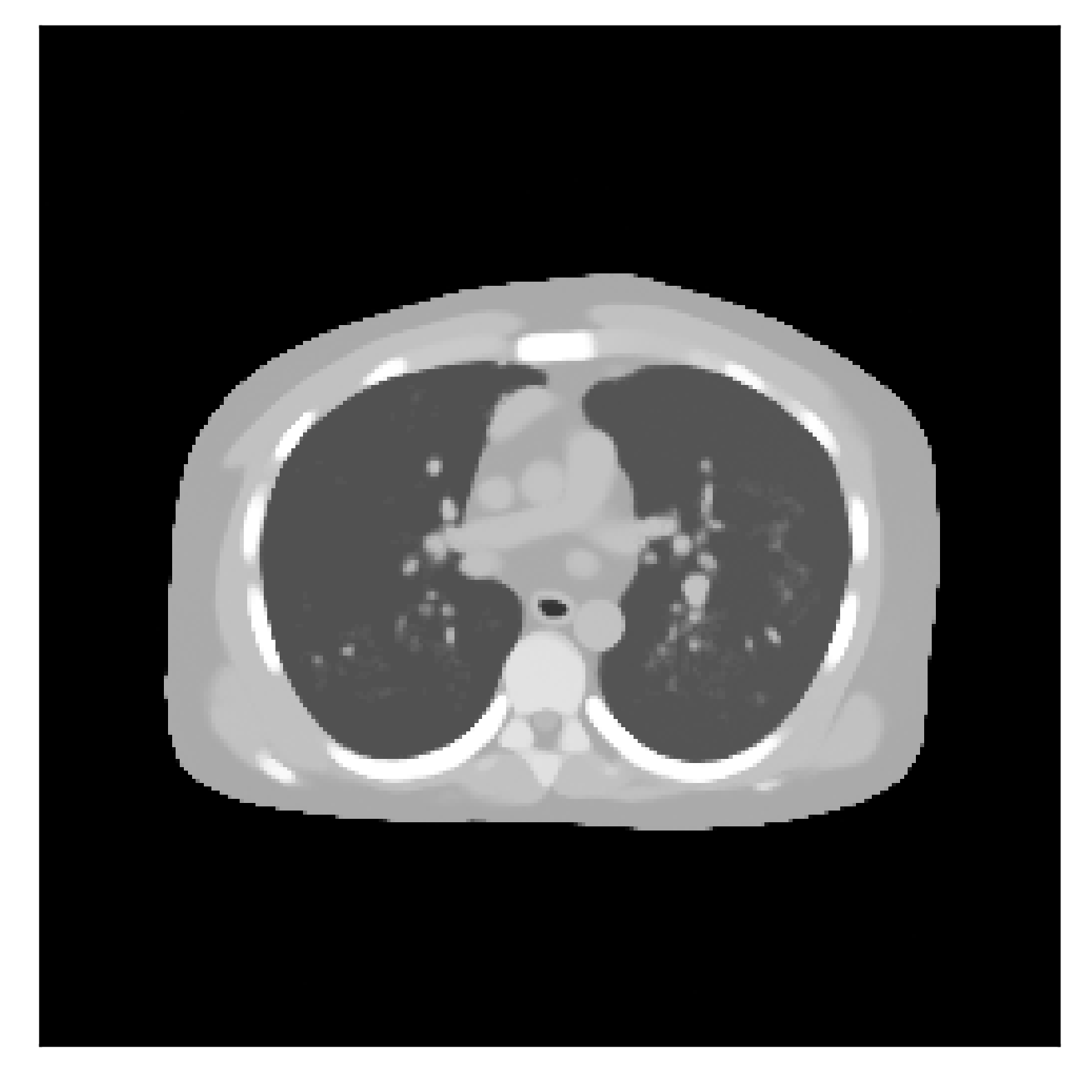
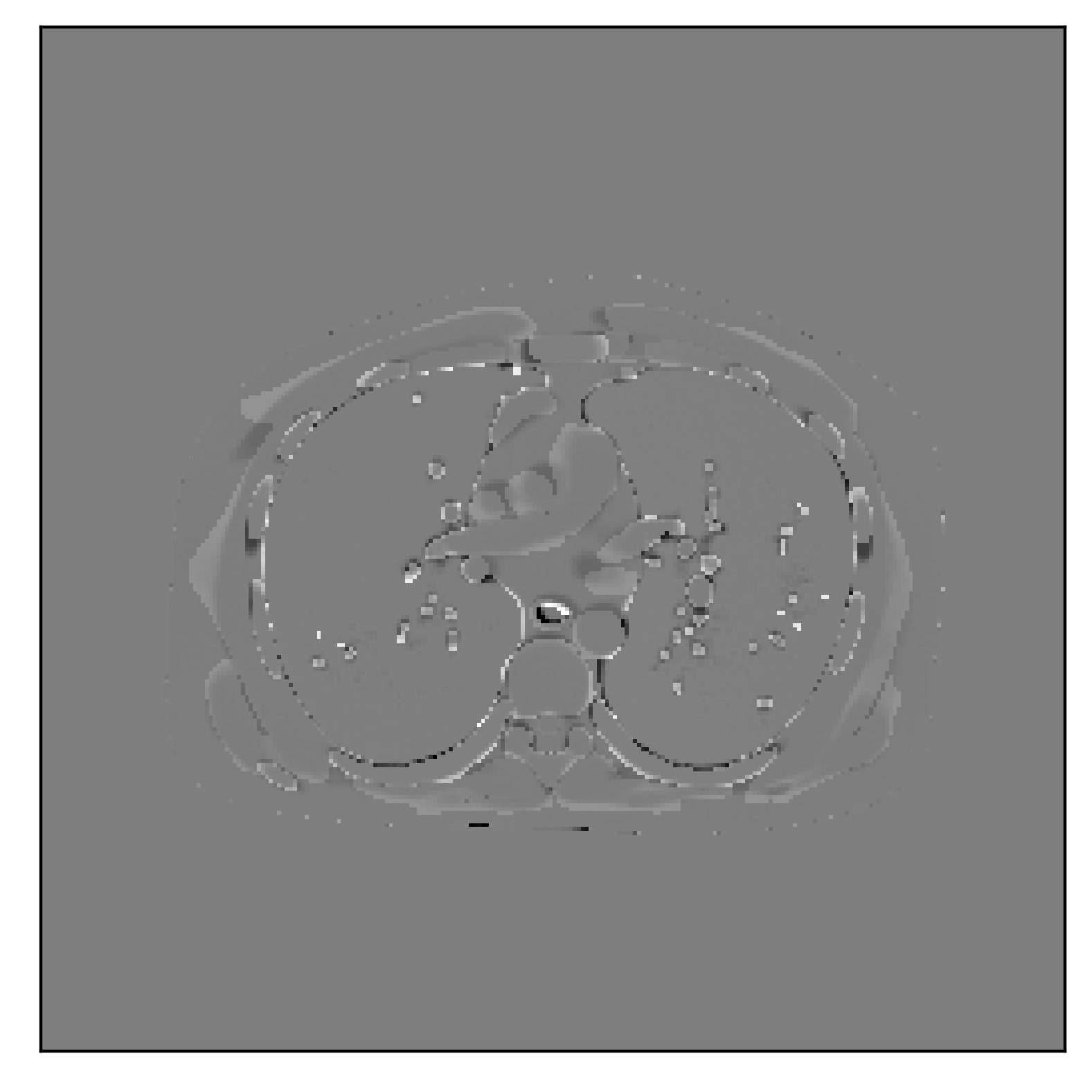
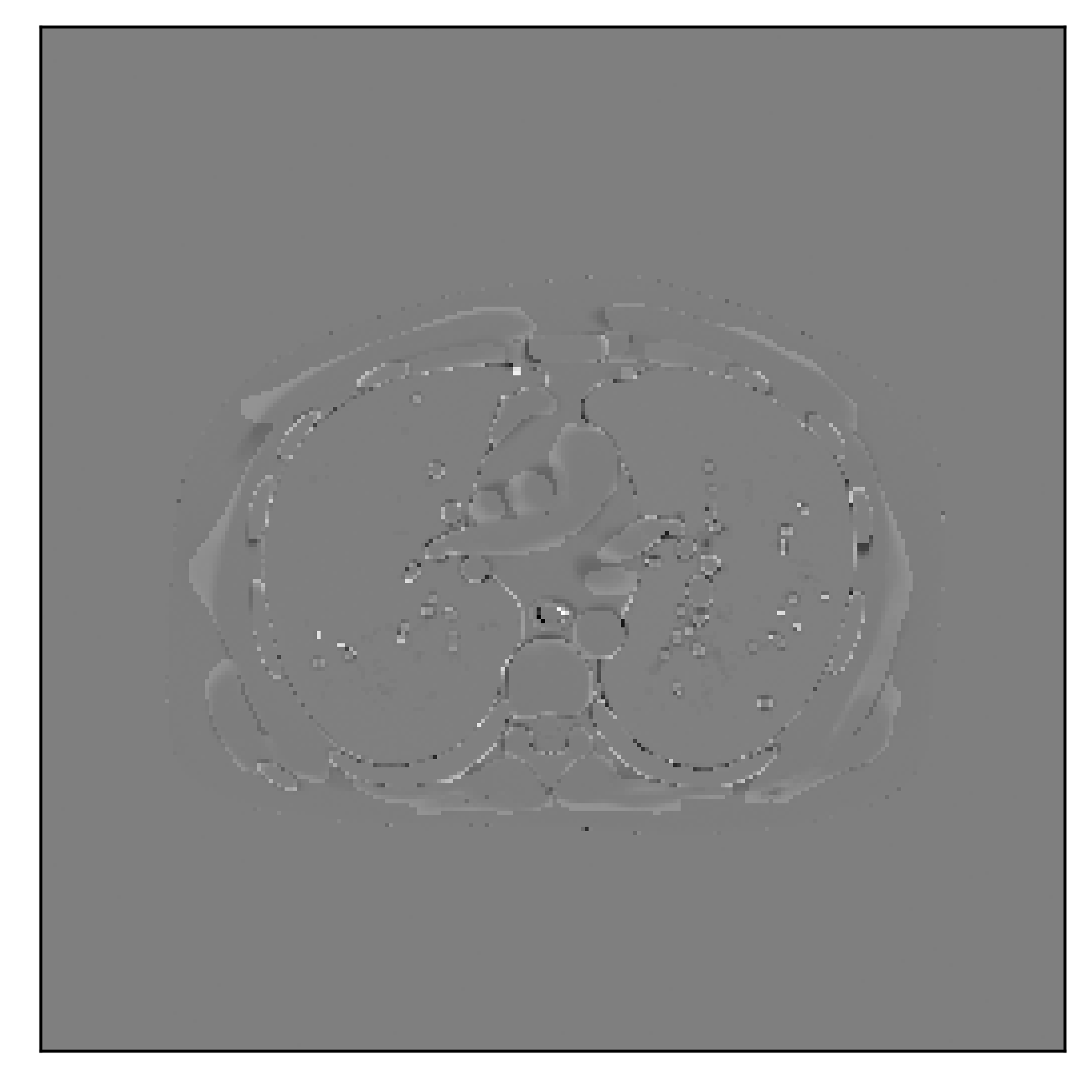
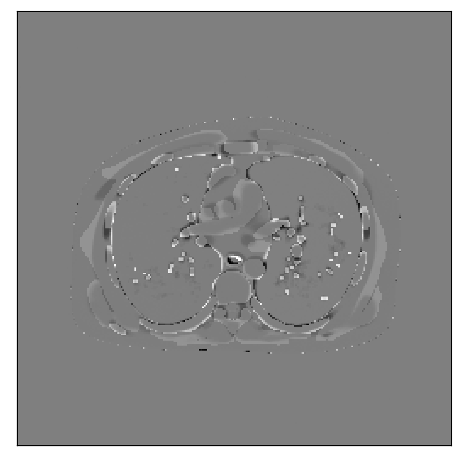
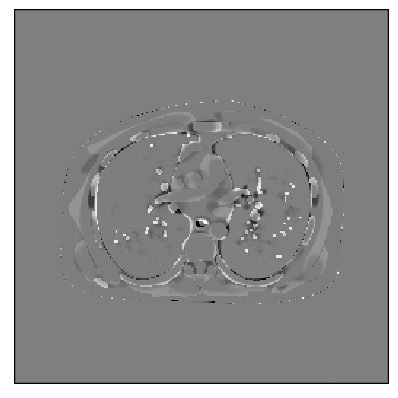
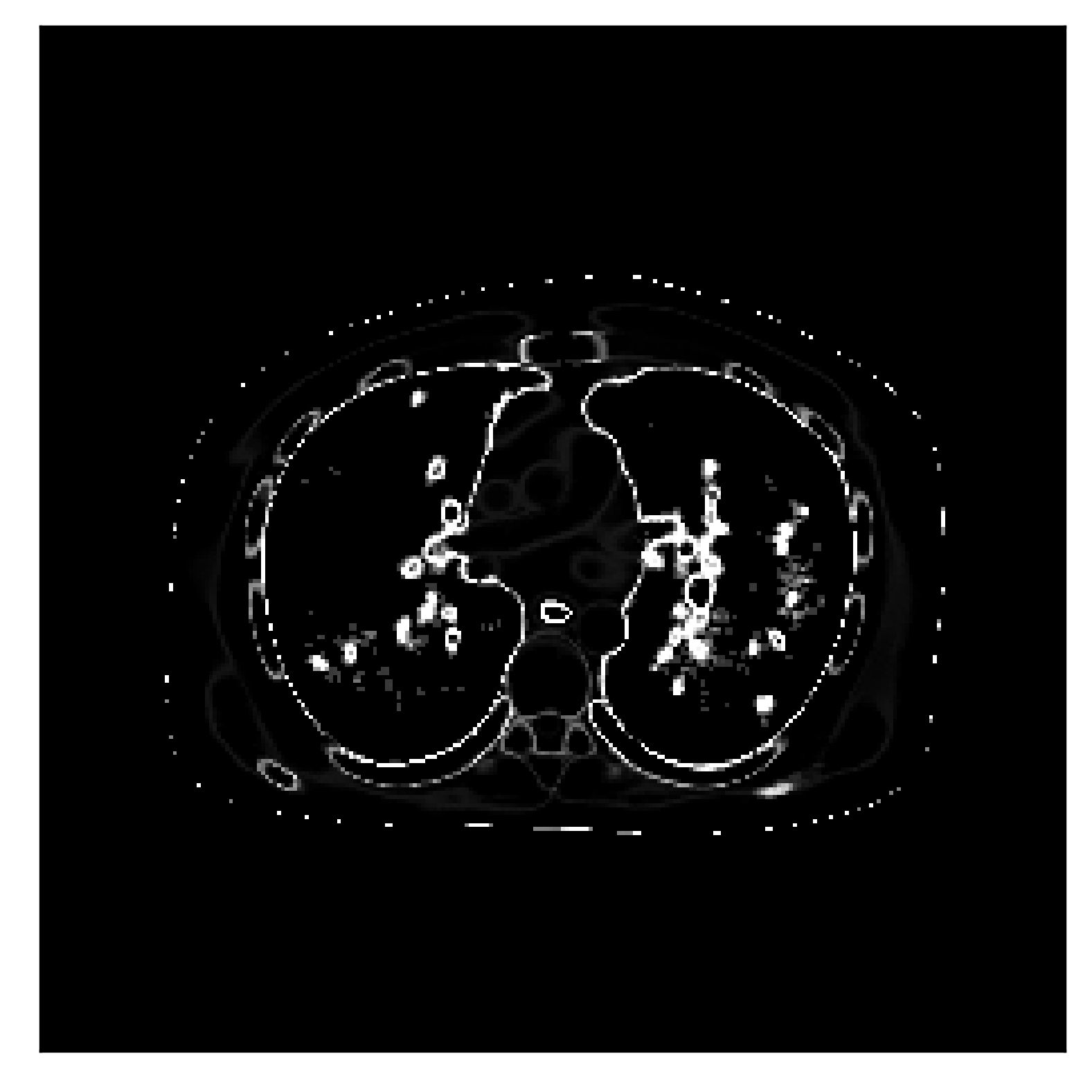
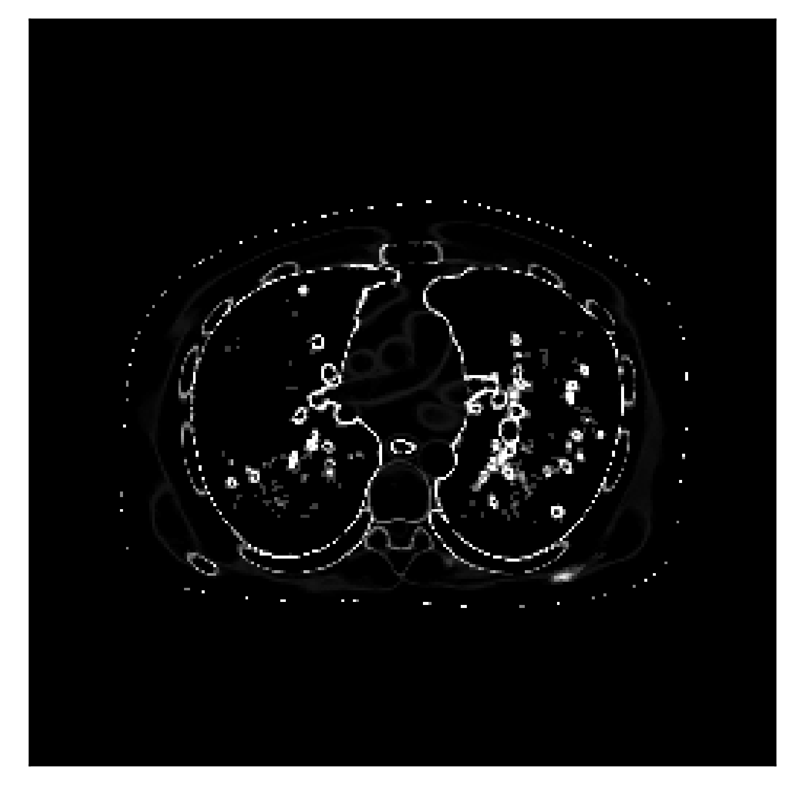
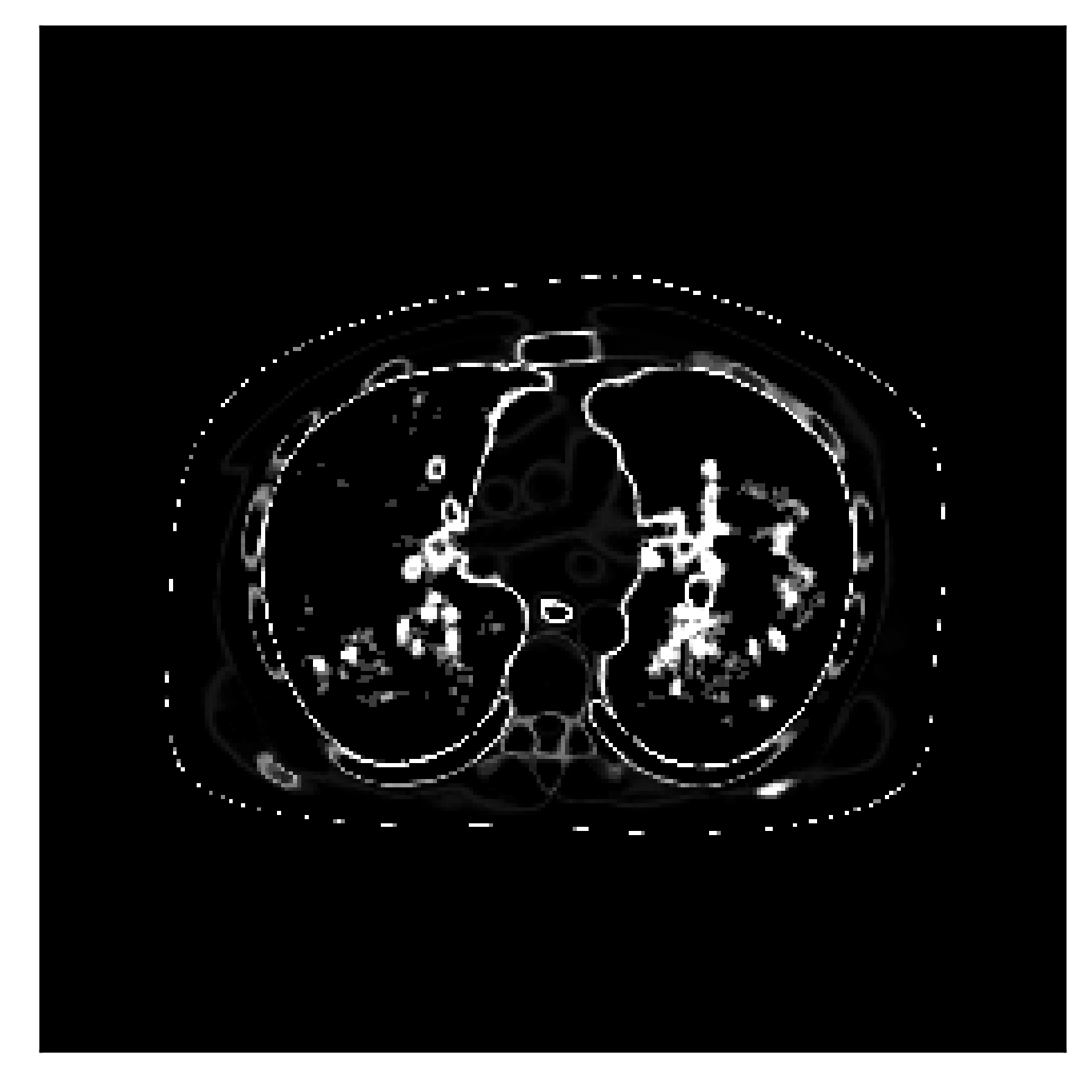
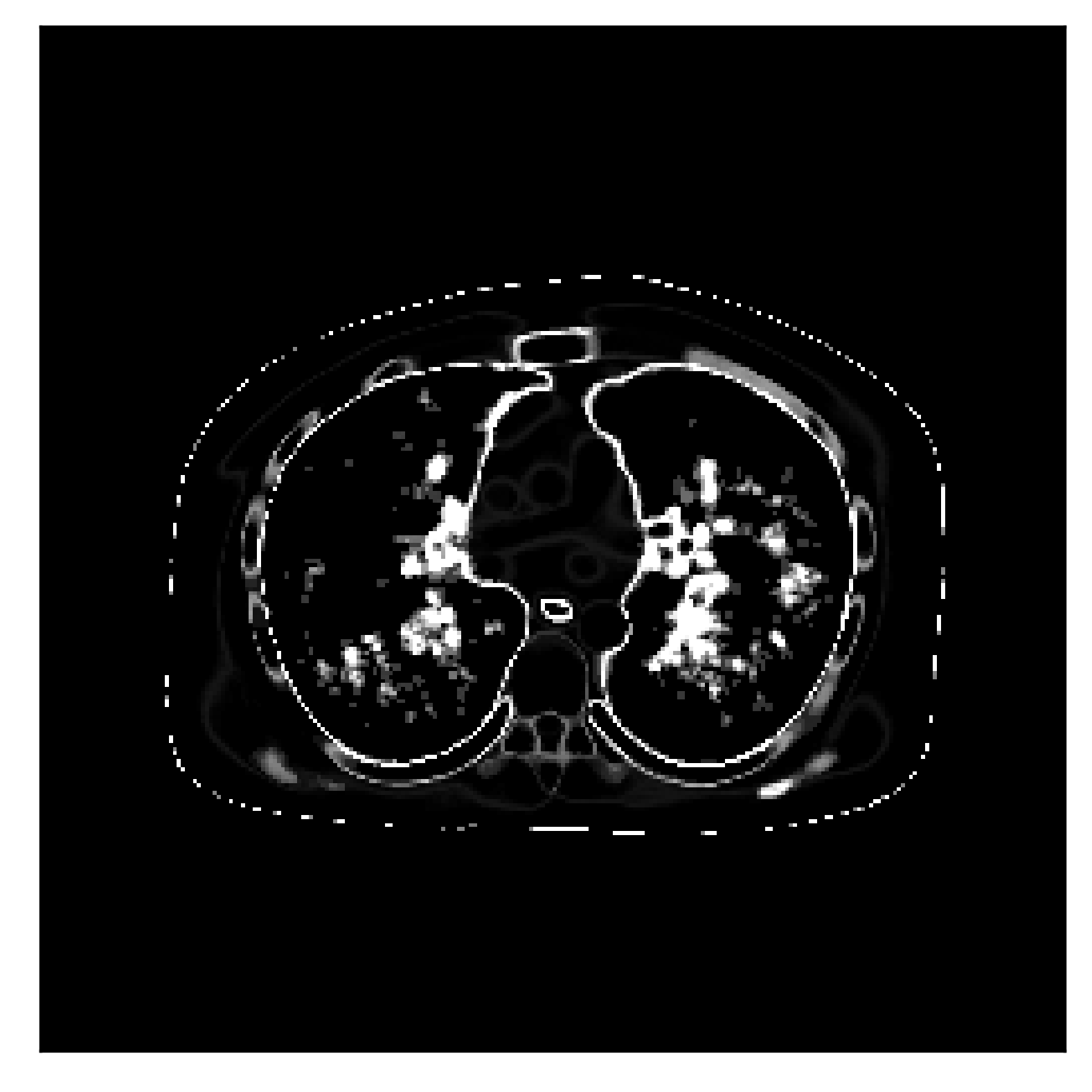
To visualize OS-DPS reconstruction results, we chose to plot the mean, bias, and standard deviation images for a sampling of different numbers of ordered subsets (equal to 1, 6, 24, and 48). These results are shown in Figure 6. Again, the highest variability across all approaches lies in small lung features and at tissue boundaries. In general there appears to be an increase both in variability and bias as larger number of subsets are used. Interestingly, the six subset scenario appear that it might have some regional decreases in variability and bias relative to the single subset scenario, but this not evident in the previously computed PSNR (which is computed over the entire image).

Figure 7 demonstrates OS-DPS Nonlinear performance for only $200$ iterations for different numbers of ordered subsets. All of the results are generated in around 20 seconds, which is significantly faster than the $1000$ iteration case. Despite the limited computation time, the reconstructed data appear qualitatively similar to previous results. We found that OS-DPS Nonlinear achieved a PSNR of $42.48$ dB for 4 subsets, $43.83$ dB for 8 subsets, $44.33$ dB for 20 subsets. Similarly, the SSIM for 4 subsets was $0.3481$, 8 subsets was $0.3601$, and 20 subsets was $0.3730$. Though subtle in a subjective evaluation of the images, these quantitative results suggest that ordered-subsets can improve the image quality when computation time is limited.

Figure 7: Combined CT reconstructions comparing, 4 subsets, 8 subsets, and 20 subsets. Colormap: W/L = 2000/0 HU. These results are generated within only $200$ iterations of OS-DPS.

4 Discussion and Conclusion

We have demonstrated a new application of diffusion posterior sampling where a nonlinear measurement model is specified to combine prior knowledge of CT imagery from unsupervised training with a reverse process that is conditioned on the data likelihood model. We demonstrate the technique on two different measurement models to illustrate the application of DPS Nonlinear without the need for re-training for different measurement processes. We observe better performance than classic reconstruction methods; however, we also see the hallucinations that are possible with this and other generative approaches. How to address, analyze, and present data from generative methods remains an extremely important research area. In an investigation of the ordered-subsets variant of DPS Nonlinear, we found that OS-DPS Nonlinear does permit modest gains in terms of computational speedup and/or image quality (in a scenario of limited reconstruction time). We note that our implementation of DPS Nonlinear was careful to use projectors and backprojectors that are PyTorch compliant to reduce inefficiencies associated with GPU-CPU transfers or other data formatting issues. While these computational advantages may be enhanced with a more thorough optimization of all algorithm parameters and may be more significant for larger (e.g. 3D reconstruction) datasets; these results also suggest the need for acceleration of the computations associated with the reverse diffusion process.

In general, this initial study on DPS Nonlinear shows great promise; however, many aspects are not fully investigated. For example, a more comprehensive investigation of important algorithmic elements is required including selection of $\lambda$ and the required number of time steps, as these can have an impact on the balance between the prior and the data likelihood, as well as the output image quality.

While the preliminary data shown here illustrate the basic potential of the DPS approach, the prospects for DPS Nonlinear application across imaging systems is very broad. We continue to investigate applications where the nonlinear model is a critical element to reconstruction. For example, measurement models that exhibit significant detector blur are difficult (or impossible) to linearize - making the DPS Nonlinear approach an attractive option for reconstruction.

ACKNOWLEDGEMENTS: This work was supported, in part, by NIH grant R01CA249538. Thanks to Xiaoxuan Zhang (University of Pennsylvania, Philadelphia, PA, USA), Peiqing Teng (Johns Hopkins University, Baltimore, MD, USA), Xiao Jiang (Johns Hopkins University, Baltimore, MD, USA) for their contributions.

References

- [1] Kang, E., Min, J., and Ye, J. C., “A deep convolutional neural network using directional wavelets for low-dose x-ray ct reconstruction,” Medical physics 44(10), e360–e375 (2017).
- [2] Wu, D., Kim, K., El Fakhri, G., and Li, Q., “Iterative low-dose ct reconstruction with priors trained by artificial neural network,” IEEE transactions on medical imaging 36(12), 2479–2486 (2017).
- [3] Jing, J., Xia, W., Hou, M., Chen, H., Liu, Y., Zhou, J., and Zhang, Y., “Training low dose ct denoising network without high quality reference data,” Physics in Medicine & Biology 67(8), 084002 (2022).
- [4] Kazerouni, A., Aghdam, E. K., Heidari, M., Azad, R., Fayyaz, M., Hacihaliloglu, I., and Merhof, D., “Diffusion models in medical imaging: A comprehensive survey,” Medical Image Analysis , 102846 (2023).
- [5] Chung, H., Sim, B., Ryu, D., and Ye, J. C., “Improving diffusion models for inverse problems using manifold constraints,” Advances in Neural Information Processing Systems 35, 25683–25696 (2022).
- [6] Müller-Franzes, G., Niehues, J. M., Khader, F., Arasteh, S. T., Haarburger, C., Kuhl, C., Wang, T., Han, T., Nebelung, S., Kather, J. N., et al., “Diffusion probabilistic models beat gans on medical images,” arXiv preprint arXiv:2212.07501 (2022).
- [7] Liu, J., Anirudh, R., Thiagarajan, J. J., He, S., Mohan, K. A., Kamilov, U. S., and Kim, H., “Dolce: A model-based probabilistic diffusion framework for limited-angle ct reconstruction,” arXiv preprint arXiv:2211.12340 (2022).
- [8] Xia, W., Cong, W., and Wang, G., “Patch-based denoising diffusion probabilistic model for sparse-view ct reconstruction,” arXiv preprint arXiv:2211.10388 (2022).
- [9] Ho, J., Jain, A., and Abbeel, P., “Denoising diffusion probabilistic models,” Advances in neural information processing systems 33, 6840–6851 (2020).
- [10] Song, Y., Sohl-Dickstein, J., Kingma, D. P., Kumar, A., Ermon, S., and Poole, B., “Score-based generative modeling through stochastic differential equations,” arXiv preprint arXiv:2011.13456 (2020).
- [11] Tivnan, M., Teneggi, J., Lee, T.-C., Zhang, R., Boedeker, K., Cai, L., Gang, G. J., Sulam, J., and Stayman, J. W., “Fourier diffusion models: A method to control mtf and nps in score-based stochastic image generation,” arXiv preprint arXiv:2303.13285 (2023).
- [12] Song, Y., Shen, L., Xing, L., and Ermon, S., “Solving inverse problems in medical imaging with score-based generative models,” arXiv preprint arXiv:2111.08005 (2021).
- [13] Chung, H., Kim, J., Mccann, M. T., Klasky, M. L., and Ye, J. C., “Diffusion posterior sampling for general noisy inverse problems,” arXiv preprint arXiv:2209.14687 (2022).
- [14] Lopez Montes, A., McSkimming, T., Zbijewksi, W., Skeats, A., Delnooz, C., Siewerdsen, J., and Sisneiga, A., “Diffusion posterior sampling-based reconstruction for stationary ct imaging of intracranial hemorrhage,” in [Int’l Mtg. on Fully 3D Image Recon in Rad. & Nuc. Med. ], (2023).
- [15] Bushe, D., Zhang, R., Chen, G.-H., and Li, K., “Unbiased zero-count correction method in low-dose high-resolution photon counting detector ct,” Physics in Medicine & Biology 68(11), 115002 (2023).
- [16] Hsieh, J., Molthen, R. C., Dawson, C. A., and Johnson, R. H., “An iterative approach to the beam hardening correction in cone beam ct,” Medical physics 27(1), 23–29 (2000).
- [17] Tilley, S., Siewerdsen, J. H., and Stayman, J. W., “Model-based iterative reconstruction for flat-panel cone-beam ct with focal spot blur, detector blur, and correlated noise,” Physics in Medicine & Biology 61(1), 296 (2015).
- [18] Hyvärinen, A. and Dayan, P., “Estimation of non-normalized statistical models by score matching.,” Journal of Machine Learning Research 6(4) (2005).
- [19] Tilley, S., Jacobson, M., Cao, Q., Brehler, M., Sisniega, A., Zbijewski, W., and Stayman, J. W., “Penalized-likelihood reconstruction with high-fidelity measurement models for high-resolution cone-beam imaging,” IEEE transactions on medical imaging 37(4), 988–999 (2017).
- [20] Ronneberger, O., Fischer, P., and Brox, T., “U-net: Convolutional networks for biomedical image segmentation,” in [MICCAI 2015 ], 234–241, Springer (2015).
- [21] Segars, W. P., Sturgeon, G., Mendonca, S., Grimes, J., and Tsui, B. M., “4d xcat phantom for multimodality imaging research,” Medical physics 37(9), 4902–4915 (2010).
- [22] Xia, W., Shi, Y., Niu, C., Cong, W., and Wang, G., “Diffusion prior regularized iterative reconstruction for low-dose ct,” arXiv preprint arXiv:2310.06949 (2023).
- [23] Erdogan, H. and Fessler, J. A., “Ordered subsets algorithms for transmission tomography,” Physics in Medicine & Biology 44(11), 2835 (1999).
- [24] Ahn, S. and Fessler, J. A., “Globally convergent image reconstruction for emission tomography using relaxed ordered subsets algorithms,” IEEE transactions on medical imaging 22(5), 613–626 (2003).
- [25] Hudson, H. M. and Larkin, R. S., “Accelerated image reconstruction using ordered subsets of projection data,” IEEE transactions on medical imaging 13(4), 601–609 (1994).
- [26] Kim, H. and Champley, K., “Differentiable forward projector for x-ray computed tomography,” arXiv preprint arXiv:2307.05801 (2023).