Uncertainty-biased molecular dynamics for learning uniformly accurate interatomic potentials

Abstract

Efficiently creating a concise but comprehensive data set for training machine-learned interatomic potentials (MLIPs) is an under-explored problem. Active learning (AL), which uses either biased or unbiased molecular dynamics (MD) simulations to generate candidate pools, aims to address this objective. Existing biased and unbiased MD simulations, however, are prone to miss either rare events or extrapolative regions—areas of the configurational space where unreliable predictions are made. Simultaneously exploring both regions is necessary for developing uniformly accurate MLIPs. In this work, we demonstrate that MD simulations, when biased by the MLIP’s energy uncertainty, effectively capture extrapolative regions and rare events without the need to know a priori the system’s transition temperatures and pressures. Exploiting automatic differentiation, we enhance bias-forces-driven MD simulations by introducing the concept of bias stress. We also employ calibrated ensemble-free uncertainties derived from sketched gradient features to yield MLIPs with similar or better accuracy than ensemble-based uncertainty methods at a lower computational cost. We use the proposed uncertainty-driven AL approach to develop MLIPs for two benchmark systems: alanine dipeptide and MIL-53(Al). Compared to MLIPs trained with conventional MD simulations, MLIPs trained with the proposed data-generation method more accurately represent the relevant configurational space for both atomic systems.

Introduction

Computational techniques are invaluable for exploring complex configurational and compositional spaces of molecular and material systems. The accuracy and efficiency, however, depend on the chosen computational methods. Ab initio molecular dynamics (AIMD) simulations using density-functional theory (DFT) provide accurate results but are computationally demanding. Atomistic simulations with classical force fields (FFs) offer a faster alternative but often lack accuracy. Thus, developing accurate and computationally efficient interatomic potentials is a key challenge that has been successfully addressed by machine-learned interatomic potentials (MLIPs).[1, 2, 3] An essential component of any MLIP is the accurate encoding of the atomic system by a local representation, which depends on configurational (atomic positions) and compositional (atomic types) degrees of freedom.[4] Recently, a wide range of machine learning approaches have been introduced, including linear and kernel-based models,[5, 6, 7, 8] Gaussian approximation,[9, 10] and neural network (NN) interatomic potentials,[11, 12, 13, 14, 15, 16, 17, 18] all demonstrating remarkable success in atomistic simulations.

The effectiveness of MLIPs, however, crucially relies on training data sufficiently covering the relevant configurational and compositional spaces.[19, 20] Without such training data, MLIPs cannot faithfully reproduce the underlying physics. An open challenge, therefore, is the generation of comprehensive training data sets for MLIPs, covering relevant configurational and compositional spaces and ensuring that resulting MLIPs are uniformly accurate across these spaces. This objective must be realized while reducing the number of expensive DFT evaluations, which provide reference energies, atomic forces, and stresses. This challenge is further complicated by the limited knowledge of physical conditions, such as temperature and pressure, at which configurational changes occur.

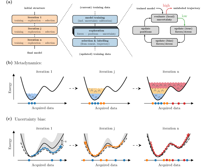
Figure 1: A schematic overview of an AL algorithm for MLIP training. Training structures are selected from data gathered during biased or unbiased MD simulations. (a) An AL experiment begins with training an MLIP in the first iteration using a small set of randomly perturbed initial configurations. The current MLIP is employed in each iteration to run parallel MD simulations. Each simulation continues until it reaches a predefined uncertainty threshold. Then, a batch of configurations is selected from all trajectories. Reference energies and forces of these samples are evaluated using a DFT solver, updating the training data set. The updated data set is employed for training the MLIP in the next iteration. (b) Adaptive biasing strategies like metadynamics enhance the exploration of the configurational space. In metadynamics, exploration along manually defined CVs is facilitated by adding Gaussian functions to a history-dependent bias (areas filled by blue, orange, and red colors). However, even for well-defined CVs, exploring the configurational space of interest may require long simulation times due to the diffusive motion along these CVs. (c) Uncertainty-biased MD aims to minimize uncertainty $u$ (grey shaded area) related to the actual error, thereby facilitating the exploration of the configurational space. In uncertainty-biased MD, we subtract the MLIP’s energy uncertainty from the predicted energy (continuous black line) and run MD simulations using the altered energy surface (dashed black line). Curved lines denote distinct MD trajectories. Unlike metadynamics, uncertainty-biased MD operates without defining CVs and drives MD simulations toward high uncertainty regions in each iteration.

To address this challenge, iterative active learning (AL) algorithms can be used to improve the accuracy of MLIPs by providing an augmented data set;[21, 22, 23, 24, 25, 26] see Fig. 1 (a). They select the data most informative to the model, that is, atomic configurations with higher energy and force uncertainties, as estimated by the model. This data is drawn from configurational and compositional spaces explored during, e.g., molecular dynamics (MD) simulations. Reference DFT energies, atomic forces, and stresses are evaluated for the selected atomic configurations. Furthermore, energy and force uncertainties indicate the onset of extrapolative regions—regions where unreliable predictions are made—prompting the termination of the MD simulation and the evaluation of reference DFT values. In such a naive AL setting, covering the configurational space and exploring extrapolative configurations might require running longer MD simulations and defining physical conditions for observing slow configurational changes (rare events).

Alternatively, enhanced sampling methods can significantly speed up the exploration of the configurational space by using adaptive biasing strategies such as metadynamics;[27, 28, 29, 30, 31, 32] see Fig. 1 (b). However, metadynamics requires manually selecting a few collective variables (CVs) which are assumed to describe the system. The limited number of CVs restricts exploration, as they might miss relevant transitions and parts of the configurational space. In contrast, MD simulations biased toward regions of high uncertainty can enhance the discovery of extrapolative configurations.[33, 34] A related work utilizes uncertainty gradients with respect to atomic positions for adversarial training of MLIPs.[35] To obtain MLIPs that are uniformly accurate across the relevant configurational space, however, efficient exploration of both rare events and extrapolative configurations is necessary. The extent to which uncertainty-biased MD can achieve this objective remains an unexplored research area.

In this work, we demonstrate the capability of uncertainty-biased MD to explore the relevant configurational space, including fast exploration of rare events and extrapolative regions; see Fig. 1 (c). We achieve this by exploring the CVs of alanine dipeptide—a widely used model for protein backbone structure. To assess the coverage of the CV space, we introduce a measure using a tree-based weighted recursive space partitioning. Furthermore, we extend existing uncertainty-biased MD simulations by automatic differentiation (AD) and propose a novel biasing technique that utilizes bias stresses obtained by differentiating the model’s uncertainty with respect to infinitesimal strain deformations. We assess the efficiency of the proposed biasing technique by running MD simulations at constant pressure ($NpT$ statistical ensemble) and exploring cell parameters of MIL-53(Al)—a flexible metal-organic framework (MOF) featuring closed- and large-pore stable states.

A key ingredient of any uncertainty-driven AL algorithm is a sensitive measure of local structural changes for detecting the onset of extrapolative regions. However, MLIP uncertainties often underestimate actual errors, resulting in the exploration of unphysical regions, negatively affecting MLIP training. Thus, calibrated uncertainties are crucial for learning high-quality MLIPs in a data-driven manner. In our setting, we demonstrate that conformal prediction (CP) helps align the highest force error with its corresponding uncertainty value. This approach effectively makes MLIPs not underestimate force errors, which is important for preventing MD simulations from exploring unphysical configurations. Thus, CP-based uncertainty calibration helps set reasonable uncertainty thresholds without limiting the exploration of the configurational space. In contrast, conventional approaches drive MD away from high-uncertainty regions, which can hinder exploration.[36]

Contrary to existing work,[33, 34] which relies on ensembles of MLIPs for uncertainty quantification, we use ensemble-free uncertainties of NN-based MLIPs derived from gradient features.[37, 38, 39] These features can be interpreted as the sensitivity of a model’s output to changes in its parameters. We demonstrate that gradient features can be used to define uncertainties of total and atom-based properties, such as energy and atomic forces. To make gradient-based uncertainties computationally efficient, we employ the sketching technique[40] and reduce the dimensionality of gradient features.

We further enhance configurational space exploration and improve the computational efficiency of uncertainty-driven AL by employing batch selection algorithms.[38, 39] These algorithms simultaneously select multiple atomic configurations from trajectories generated during parallel MD simulations. Batch selection algorithms enforce the informativeness and diversity of the selected atomic structures. Thus, they ensure the construction of maximally diverse training data sets.

Results

In the following, we first demonstrate the necessity of uncertainty calibration on an example of MIL-53(Al) to constrain MD simulations to physically reasonable regions of the configurational space. Then, we present two complementary analyses demonstrating the improved data efficiency of MLIPs obtained by our uncertainty-driven AL approach, developing MLIPs for alanine dipeptide and MIL-53(Al). Furthermore, we investigate how uncertainty-biased MD enhances the exploration of the configurational space, utilizing bias forces and stress. To benchmark our results, we draw a comparison with MD run at elevated temperatures and pressures as well as metadynamics simulations. The details on the ensemble-free uncertainties (distance- and posterior-based ones derived from sketched gradient features) and uncertainty-biased MD can be found in the Methods section.

Calibrating uncertainties with conformal prediction

Total and atom-based uncertainties are typically poorly calibrated,[41] meaning that they often underestimate actual errors. The underestimation of errors is particularly dangerous when dynamically generating candidate pools, as it may result in exploring unphysical configurations. Specifically, poor calibration complicates defining an appropriate uncertainty threshold for prompting the termination of MD simulations and the evaluation of reference DFT energies, atomic forces, and stresses. To address this issue, we utilize inductive CP, which computes a re-scaling factor based on predicted uncertainties and prediction errors on a calibration set. The confidence level $1-\alpha$ in CP is defined such that the probability of underestimating the error is at most $\alpha$ on data drawn from the same distribution as the calibration set. The detailed procedure can be found in the Methods section.

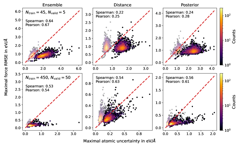
Figure 2: Correlation of maximal atom-based uncertainties with maximal atomic force RMSEs for MIL-53(Al). The results are presented for the test data set from Ref. 32. All uncertainty quantification methods are calibrated using CP and atomic force RMSEs. The top row shows the results of MLIPs trained using 45 atomic configurations, while five are additionally used for early stopping and uncertainty calibration. The bottom row shows the results obtained with $450$ and $50$ MIL-53(Al) configurations, respectively. The training and validation data are taken from Ref. 32. Transparent hexbin points represent uncertainties calibrated with $\alpha=0.5$ (low confidence; see Methods), while opaque ones denote uncertainties calibrated with $\alpha=0.05$ (high confidence). Calibrating uncertainties with a high confidence level helps align the largest actual error with the corresponding uncertainty, shifting the hexbin points to or below the red diagonal line. This alignment is crucial for identifying unreliable predictions and prompting the termination of MD simulations.

Figure 2 demonstrates the correlation of maximal atom-based uncertainties with maximal atomic force RMSEs for the MIL-53(Al) test data set from Ref. 32. In the figure, transparent hexbins represent uncertainties calibrated with a lower confidence ($\alpha=0.5$; see Methods), while opaque ones depict those calibrated with a higher confidence ($\alpha=0.05$). The presented uncertainties are derived from gradient features or an ensemble of three MLIPs (see Methods) and calibrated using CP with atomic force RMSEs. For posterior- and distance-based uncertainties, which are unitless, the re-scaling with CP ensures that the resulting uncertainties are provided in correct units, i.e., eV/Å. Ensemble-based uncertainty quantification already provides correct units, which are preserved by CP. Equivalent results for alanine dipeptide can be found in the Supplementary Information.

Figure 2 (top) demonstrates results for MLIPs trained on 45 MIL-53(Al) configurations, while five samples were additionally used for early stopping and uncertainty calibration. Figure 2 (bottom) shows the results for MLIPs trained and validated on 450 and 50 MIL-53(Al) configurations, respectively. In both experiments, the training and validation samples were selected from the data sets provided by Ref. 32. The first 50 samples correspond to randomly perturbed MIL-53(Al) structures, while the remaining 450 are generated using metadynamics combined with the incremental learning approach.[32] The latter is an iterative learning algorithm that improves MLIPs by training on configurations generated sequentially over time, explicitly using the last simulation frame of atomistic simulations.

We observe that uncertainties calibrated with a lower confidence level often underestimate actual errors. In this case, MD simulations can explore unphysical regions before reaching the uncertainty threshold, especially in cases with a small correlation between uncertainties and actual errors. By employing CP with higher confidence, we help align the largest prediction error with the corresponding uncertainty, thereby improving its ability to identify the onset of extrapolative regions. This alignment becomes apparent in Fig. 2, where CP shifts the hexbin points to be on or below the diagonal line.

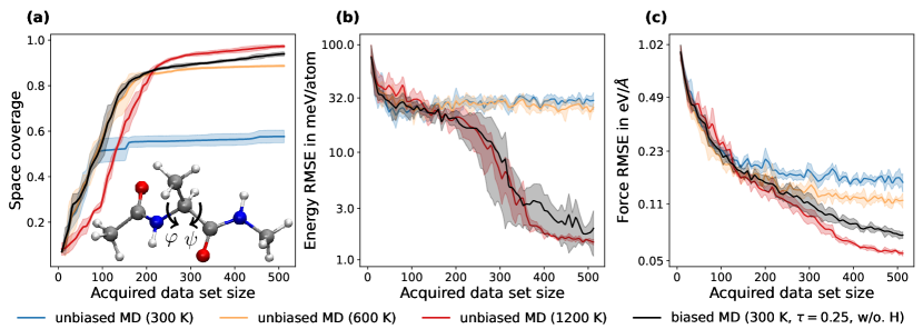
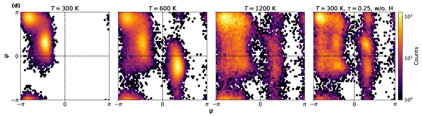
Figure 3: Comparison of AL approaches employing biased and unbiased MD simulations to generate the candidate pool of atomic configurations for alanine dipeptide. Results are provided for the posterior-based uncertainty quantification derived from sketched gradient features. Unlike unbiased MD simulations, which rely on atom-based uncertainties to terminate MD simulations, biased MD simulations use both total and atom-based uncertainties for biasing MD simulations and prompting their termination, respectively. We use three metrics to assess the performance of our AL approaches: (a) Coverage of the CV space; (b) Energy RMSE; and (c) Force RMSE. All RMSEs are evaluated on the alanine dipeptide test data set; see Methods. Shaded areas denote the standard deviation across five independent runs. The alanine dipeptide molecule, including its CVs, is shown as an inset in (a). The color code of the inset molecule is C grey, O red, N blue, and H white. (d) Ramachandran plots demonstrating the CV spaces explored by the four AL experiments. Biased MD simulations achieve exceptional performance, close to those of MD simulations conducted at 1200 K, without a priori knowledge of transition temperatures between stable states. The CV space covered by uncertainty-biased MD simulations at 300 K matches that of unbiased simulations at 1200 K, significantly outperforming the coverage achieved by unbiased MD simulations at 300 K and 600 K.

Table 1: CV space coverage, atomic energy (E-) and atomic force (F-) RMSEs, as well as position (Pos.) and uncertainty (Unc.) ACTs for alanine dipeptide experiments conducted with posterior-based uncertainties. CV space coverage, E- and F-RMSEs are reported for MLIPs obtained at the end of each experiment, while ACTs are computed using the entire trajectory obtained throughout the experiment. E-RMSE is given in meV/atom, while F-RMSE is in eV/Å. ACTs are provided in ps. For biased MD, we compare two cases: one with (w.) biasing hydrogen atoms and one without (w/o.).

Experiment	CV space cov.	E-RMSE	F-RMSE	Pos. ACT	Unc. ACT
unbiased MD (300 K)	0.58 $\pm$ 0.03	30.29 $\pm$ 5.47	0.149 $\pm$ 0.019	2.07 $\pm$ 0.11	327.11 $\pm$ 8.69
unbiased MD (600 K)	0.89 $\pm$ 0.00	26.03 $\pm$ 2.23	0.116 $\pm$ 0.012	1.23 $\pm$ 0.02	257.88 $\pm$ 22.01
unbiased MD (1200 K)	0.97 $\pm$ 0.01	1.47 $\pm$ 0.09	0.055 $\pm$ 0.002	0.74 $\pm$ 0.02	21.41 $\pm$ 4.91
biased MD (300 K, $\tau=0.25$, w. H)	0.87 $\pm$ 0.02	5.09 $\pm$ 5.40	0.082 $\pm$ 0.016	2.08 $\pm$ 0.13	19.38 $\pm$ 7.42
biased MD (300 K, $\tau=0.25$, w/o. H)	0.94 $\pm$ 0.01	1.97 $\pm$ 0.88	0.071 $\pm$ 0.003	0.69 $\pm$ 0.04	52.79 $\pm$ 19.40

In Fig. 2 (top), we find that even training and calibrating models with a small set of randomly perturbed atomic configurations is sufficient for robust identification of unreliable predictions. This result is crucial as we rely on such data sets to initialize our AL experiments, eliminating the need for predefined data sets.[33, 34] Furthermore, we observe that calibrated uncertainties from model ensembles tend to overestimate the actual error to a greater extent compared to gradient-based approaches. While this may not be critical when exploring unphysical configurations, it can be wasteful, leading to a premature termination of MD simulations. This trend is consistent across all training and calibration data sizes. Lastly, the results provided here and in the Supplementary Information demonstrate that all uncertainty quantification methods perform comparably regarding Pearson and Spearman correlation coefficients.

Performance of bias-forces-driven active learning

Exploring the configurational space of complex molecular systems, particularly those with multiple stable states, is essential for developing accurate and robust MLIPs. We apply bias-forces-driven MD simulations combined with AL to develop MLIPs for alanine dipeptide in vacuum. This dipeptide exhibits two stable conformers characterized by the backbone dihedral angles $\phi$ and $\psi$ (as shown in the inset of Fig. 3): the $\mathrm{C}_{\mathrm{7eq}}$ state with $\phi\approx-1.5$ rad and $\psi\approx 1.19$ rad and the $\mathrm{C}_{\mathrm{ax}}$ state with $\phi\approx 0.9$ rad and $\psi\approx-0.9$ rad.[42] We use unbiased MD simulations as the baseline to create the candidate pool for AL. We employ the AMBER ff19SB force field for reference energy and force calculations,[43] as implemented in the TorchMD package using PyTorch.[44, 45]

Each AL experiment starts with training an MLIP with eight alanine dipeptide configurations randomly perturbed from its initial configuration in the $\mathrm{C}_{\mathrm{7eq}}$ state. Trained MLIPs are then used to run eight parallel MD simulations, initialized from the initial configuration or configurations selected in later iterations. Each MD simulation runs until reaching an empirically defined uncertainty threshold of 1.5 eV/Å. A lower threshold value may result in slower CV space exploration, while a larger one would lead to the exploration of unphysical configurations. The maximum data set size, comprising training and validation data, is limited to 512 configurations. Biased (bias-forces-driven) and unbiased MD simulations are performed using the canonical ($NVT$) statistical ensemble within the ASE simulation package.[46] Unbiased MD simulations are run with the Langevin thermostat at temperatures of 300 K, 600 K, and 1200 K, whereas biased simulations are performed at a constant temperature of 300 K. We have chosen an integration time step of 0.5 fs and set a maximum of 20,000 steps for an MD simulation. A biasing strength of $\tau=0.25$ was also chosen for biased AL experiments. In reference calculations, we employ a force threshold of 20 eV/Å to exclude unphysical structures, mainly encountered at high biasing strengths (equivalently, a smaller integration time step could be used). All AL experiments have been repeated five times.

Figure 3 demonstrates the performance of MLIPs obtained for alanine dipeptide depending on the number of acquired configurations. Table 1 presents error metrics evaluated for MLIPs at the end of each experiment. Here, we provide results for the posterior-based uncertainty. Equivalent results for other uncertainty methods are presented in the Supplementary Information. Figure 3 (a) presents the coverage of the CV space defined by the two dihedral angles ($\phi$ and $\psi$). We measure the coverage of the respective space by a tree-based weighted recursive space partitioning; see Methods. AL experiments combined with unbiased MD simulations at 1200 K serve as the upper-performance limit for MLIPs in the case of alanine dipeptide, achieving the highest coverage of $0.97$ after acquiring 512 configurations. Increasing temperature even further while using interatomic potentials, which allow for bond breaking and formation, might lead to the degradation of the molecule. Uncertainty-biased MD simulations at 300 K result in slightly lower coverage values, surpassing the coverages achieved by unbiased counterparts at 300 K and 600 K.

Furthermore, biased MD simulations outperform unbiased dynamics at 1200 K, efficiently covering the CV space before acquiring about 200 configurations. This observation is attributed to the gradual increase in driving forces induced by the uncertainty bias, resulting in a more gradual distortion of the atomic structure. In contrast, high-temperature unbiased simulations perturb the system more strongly and rapidly enter extrapolative regions without exploring relevant configurational changes. Thus, high-temperature simulations may cause the degradation of the investigated atomic systems, unlike uncertainty-biased dynamics.

Figures 3 (b) and (c) present energy and force RMSEs evaluated on the alanine dipeptide test data set; see Methods. Consistent with the findings in Fig. 3 (a), AL approaches combined with biased MD simulations at 300 K outperform their unbiased counterparts at 300 K and 600 K once they acquire about 100 configurations. Biased AL experiments achieve energy RMSE of 1.97 meV/atom, close to those observed in high-temperature MD simulations, surpassing others by a factor of more than 13. A similar trend is observed for force RMSE. Biased AL experiments achieve an RMSE of 0.071 eV/Å, outperforming their counterparts at 300 K and 600 K by factors of 2.1 and 1.6, respectively. These results demonstrate the efficiency of uncertainty-biased dynamics in exploring the configurational space and developing accurate and robust MLIPs.

Biased AL experiments achieve exceptional performance without a priori knowledge of transition temperatures between stable states; see Fig. 3 (d). Defining transition temperatures requires running MD simulations at different temperatures to explore the relevant configurational space without degrading the atomic system. In contrast, there is no strong dependence of the performance of our approach on biasing strength (see the Supplementary Information), which has to be chosen within a moderate range. Our results offer evidence of rare event exploration (for alanine dipeptide, the exploration of both stable states) through uncertainty-biased dynamics. The following section will present a detailed analysis of the exploration rates.

Additionally, we have identified how to further improve our biased MD simulations by making biasing strengths species dependent; see the Supplementary Information. The results presented in this section, achieved with a biasing strength of zero for hydrogen atoms, outperform settings where all atoms are biased equally, with improvements by a factor of 1.08 in coverage and 1.15 in force RMSE; see Table 1. Thus, a more sophisticated data-driven redistribution of biasing strengths can further enhance the performance of bias-forces-driven MD simulations.

Exploration rates for collective variables of alanine dipeptide

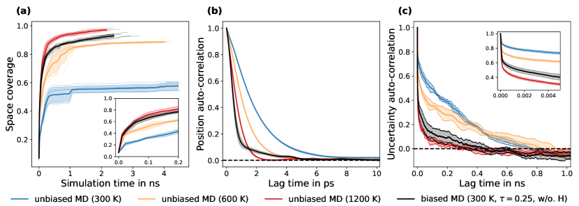
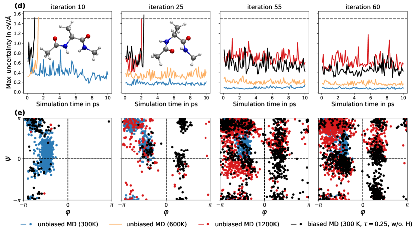
Figure 4: Evaluation of CV space exploration rates using biased and unbiased MD simulations for alanine dipeptide. Here, MD simulations generate candidate pools of atomic configurations for AL algorithms. Results are provided for the posterior-based uncertainty quantification derived from sketched gradient features. Unlike unbiased MD simulations, which rely on atom-based uncertainties to terminate MD simulations, biased MD simulations use both total and atom-based uncertainties for biasing MD simulations and prompting their termination, respectively. We use three metrics to asses the exploration rates: (a) Coverage of the CV space; (b) Auto-correlation functions of atomic positions; and (c) Auto-correlation functions of atom-based uncertainties. Shaded areas denote the standard deviation across five independent runs. (d) Time evolution of the maximal atom-based uncertainty within an AL iteration and the entire experiment. Time evolution is shown for one of the eight MD simulations. The dashed gray line represents the uncertainty threshold of 1.5 eV/Å. The insets show configurations that reached the uncertainty threshold for uncertainty-biased MD. (e) Ramachandran plots illustrate the exploration of the CV space over AL iterations and the entire experiment. Ramachandran plots are presented for unbiased MD simulations at 300 K and 1200 K and biased MD simulations at 300 K. Simulation time refers to the effective number of MD steps ($\times$ 0.5 fs) required to reach the final coverage, while lag time denotes the time interval between two successive MD frames. Biased MD simulations at 300 K exhibit at least two times higher exploration rates than their unbiased counterparts at 300 K and 600 K. Their exploration rates are comparable to those of unbiased MD simulations at 1200 K, with the advantage of gradually distorting the molecule, reducing the risk of its degradation.

We have observed that uncertainty-biased MD simulations effectively explore the configurational space of alanine dipeptide, defined by its CVs. Figure 4 evaluates the extent to which the introduced bias forces in MD simulations accelerate their exploration. In Fig. 4 (a), we present the coverage of the CV space as a function of simulation time, i.e., as a function of the effective number of MD steps. The figure demonstrates that uncertainty-driven AL experiments at 300 K outperform unbiased experiments at 300 K and 600 K. They achieve the same coverage in considerably shorter simulation times, thereby enhancing exploration rates by a factor of larger than two. At the same time, biased MD simulations yield results comparable to those obtained from unbiased MD simulations at 1200 K. Thus, we can argue that uncertainty-biased MD explores the relevant configurational space at a similar rate to unbiased MD conducted at 1200 K.

The exploration rates estimated from Fig. 4 (a) provide an approximate measure of how uncertainty-biased dynamics accelerate the exploration of the configurational space. To offer a more thorough assessment, we examine auto-correlation functions (ACFs) computed for both position and uncertainty spaces in Figures 4 (b) and (c), where a faster decay corresponds to a faster exploration of the respective space. We compute ACFs using concatenated MD trajectories from all AL iterations as they cover the explored configurational space during the entire experiment. Additionally, we calculate the auto-correlation time (ACT) for each experiment. For the definition of ACF and ACT, we refer to Methods. Table 1 presents ACTs for all AL experiments. Smaller ACTs correspond to a faster decay of ACFs, indicating a faster exploration of the respective spaces.

Using the computed ACTs, we conclude that biased AL experiments at 300 K explore position and uncertainty spaces two to six times faster than the unbiased MD simulations at 300 K and 600 K. Compared to the unbiased dynamics at 1200 K, they achieve comparable exploration rates in the position space and rates lower by a factor of two for the uncertainty space. Furthermore, we observed that biasing hydrogen atoms results in reduced uncertainty ACTs compared to the experiments where hydrogen atoms remained unbiased. However, explicitly biasing hydrogen atoms is less efficient in exploring the position space by a factor of three. Thus, shorter uncertainty ACTs of unbiased MD simulations at 1200 K can be attributed to a stronger distortion of bonds, including hydrogen atoms, resulting in fast exploration of extrapolative regions. While this effect is unfavorable for the enhanced exploration of slow modes, such as the CVs of alanine dipeptide, in a biased MD simulation, it may be necessary to consider incorporating small, non-zero biasing strengths for hydrogen atoms to ensure the robustness of MD simulations at elevated temperatures. Interestingly, we observe that uncertainty-biased MD simulations manage to sample two slow modes in alanine dipeptide, even though 27 degrees of freedom (corresponding to the heavy C, N, and O atoms) were effectively biased, demonstrating their remarkable efficiency.

To gain insight into the exploration of the CV space during the AL experiments, we refer to Figs. 4 (d) and (e), which illustrate the time evolution of the maximal atom-based uncertainty and the coverage of the sampled CV space for selected AL iterations. Biased MD simulations consistently explore configurations with higher uncertainty values than their unbiased counterparts at 300 K and 600 K. Furthermore, bias forces not only drive the exploration toward both stable states of alanine dipeptide but also facilitate transitions between them. These results are on par with unbiased MD simulations at 1200 K, indicating that MD simulations driven by bias forces reduce the uncertainty level uniformly across the relevant configurational space. Due to the direct correlation between uncertainties and actual errors, we can argue that uncertainty-driven AL generates uniformly accurate MLIPs across the relevant configurational space.

Performance of bias-stress-driven active learning

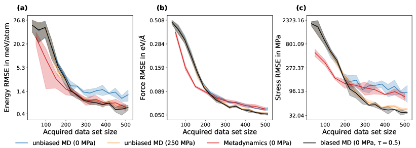
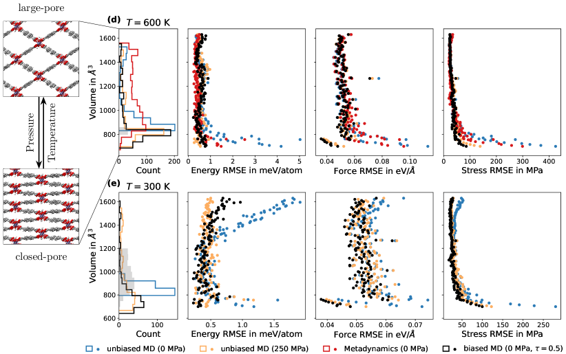
Figure 5: Comparison of AL approaches employing biased and unbiased MD simulations to generate the candidate pool of atomic configurations for MIL-53(Al). Results are provided for the posterior-based uncertainty quantification derived from sketched gradient features. Unlike unbiased MD simulations, which rely on atom-based uncertainties to terminate MD simulations, biased MD simulations use both total and atom-based uncertainties for biasing MD simulations and prompting their termination, respectively. We use three metrics to assess the performance of our AL approaches: (a) Energy RMSE; (b) Force RMSE; and (c) Stress RMSE. All RMSEs are evaluated on the MIL-53(Al) test data set.[32] Shaded areas denote the standard deviation across three independent runs, except for metadynamics. For it, shaded areas denote standard deviation across three randomly initialized MLIPs. (d) Volume distribution for atomic configurations acquired during MD at 600 K, along with volume-dependent energy, force, and stress RMSEs. (e) Volume distribution for configurations acquired during MD at 300 K, along with volume-dependent energy, force, and stress RMSEs. We employ a temperature of 300 K to reduce the probability of exploring the large-pore state of MIL-53(Al). Bias-stress-driven MD simulations outperform metadynamics-based simulations with adaptive biasing of the cell parameters. Metadynamics aims to cover the volume space uniformly. In contrast, uncertainty-biased MD generates training data sets that reduce force and stress RMSEs uniformly. Additionally, biased MD simulations enhance the exploration of closed- and large-pore states of MIL-53(Al) shown in the inset of (d).

Table 2: Atomic energy (E-), atomic force (F-), and stress (S-) RMSEs, as well as position (Pos.) and uncertainty (Unc.) ACTs for MIL-53(Al) experiments conducted with posterior-based uncertainties. E-, F-, and S-RMSEs are reported for MLIPs obtained at the end of each experiment, while ACTs are computed using the entire trajectory sampled throughout the experiment. E-RMSE is given in meV/atom, F-RMSE in eV/Å, and S-RMSE in MPa. ACTs are provided in ps.

Experiment	E-RMSE	F-RMSE	S-RMSE	Pos. ACT	Unc. ACT
$T=600$ K
unbiased MD (0 MPa)	1.17 $\pm$ 0.36	0.058 $\pm$ 0.002	90.81 $\pm$ 32.82	10.60 $\pm$ 9.54	88.05 $\pm$ 2.53
unbiased MD (250 MPa)	0.57 $\pm$ 0.05	0.052 $\pm$ 0.001	42.72 $\pm$ 1.37	2.08 $\pm$ 0.58	66.32 $\pm$ 2.02
Metadynamics (0 MPa)	0.58 $\pm$ 0.10	0.058 $\pm$ 0.002	74.83 $\pm$ 11.89	–	–
biased MD (0 MPa, $\tau=0.5$)	0.57 $\pm$ 0.08	0.051 $\pm$ 0.001	36.60 $\pm$ 1.46	2.75 $\pm$ 0.46	44.87 $\pm$ 14.08
$T=300$ K
unbiased MD (0 MPa)	0.88 $\pm$ 0.20	0.056 $\pm$ 0.001	58.57 $\pm$ 5.94	3.45 $\pm$ 4.06	99.25 $\pm$ 10.34
unbiased MD (250 MPa)	0.48 $\pm$ 0.01	0.054 $\pm$ 0.000	39.88 $\pm$ 1.76	1.86 $\pm$ 0.14	54.56 $\pm$ 4.82
biased MD (0 MPa, $\tau=0.5$)	0.49 $\pm$ 0.09	0.052 $\pm$ 0.001	33.89 $\pm$ 3.06	42.92 $\pm$ 14.18	26.89 $\pm$ 8.94

Generating training data for bulk material systems with large unit cells and multiple stable states poses a significant challenge in developing MLIPs. Therefore, we assess the performance of the bias-stress-driven AL applied to MIL-53(Al), a flexible MOF that undergoes reversible, large-amplitude volume changes under external stimuli, such as temperature and pressure (see inset of Fig. 5). MIL-53(Al) features two stable phases: the closed-pore state with a unit cell volume of $V\sim 830$ Å³ and the large-pore state with $V\sim 1419$ Å³. For reference energy, force, and stress calculations, we use the CP2K simulation package (version 2023.1)[47] and DFT at the PBE-D3(BJ) level.[48, 49] Our baseline for generating the candidate pool for AL involves unbiased MD and metadynamics,[32] which uses an adaptive biasing strategy for cell parameters of MIL-53(Al).

In each AL experiment, we start with 32 MIL-53(Al) configurations randomly perturbed around its closed-pore state, with 90 % reserved for training. Trained MLIPs are then used to perform 32 parallel MD simulations, each running until it reaches an uncertainty threshold of 1.0 eV/Å. The maximum data set size is limited to 512 configurations, comprising training and validation data. Both biased (bias-stress-driven) and unbiased MD simulations use the isobaric-isothermal form of the Nosé–Hoover dynamics.[50, 51] Unbiased MD simulations are carried out at 600 K and 0 MPa, as well as $\pm$ 250 MPa (half of the simulations each), while biased simulations are performed at 600 K and 0 MPa. The characteristic time scales of the thermostat and barostat are set to 0.1 ps and 1 ps, respectively. We have chosen an integration time step of 0.5 fs and set a maximum of 20,000 MD steps for an MD simulation. A stress-biasing strength of $\tau=0.5$ is used in biased AL experiments. In reference calculations, we employ a force threshold of 20 eV/Å to exclude strongly distorted structures. We use the data set from Ref. 32 as a metadynamics-generated baseline and select the first 500 sequentially generated configurations. All AL experiments are repeated three times, except for metadynamics, which was run once.[32] For metadynamics, we train three MLIPs initialized using different random seeds.

Figures 5 (a)–(c) demonstrate the performance of MLIPs developed for MIL-53(Al) depending on the number of acquired configurations. Table 2 presents error metrics evaluated for MLIPs at the end of each experiment. Here, we present results for the posterior-based uncertainty. Equivalent results for other uncertainty quantification methods are presented in the Supplementary Information. We observe that MLIPs trained with configurations generated using metadynamics outperform the others for data set sizes below 200 samples. This difference in performance can be attributed to how perturbed configurations are generated and the differing experimental settings between incremental learning and AL applied here. Bias-stress-driven AL outperforms metadynamics-based incremental learning after acquiring about 200 atomic configurations regarding force and stress RMSEs. Metadynamics-based experiments achieve performance on par with unbiased AL experiments conducted at 0 MPa after they reach a data set size of 200 configurations. For uncertainty-biased MD, the force RMSE improves by a factor of 1.14, and the stress RMSE improves by a factor of two. Furthermore, AL experiments employing biased MD simulations outperform unbiased MD simulations at 250 MPa regarding stress RMSE. Therefore, we can argue that bias-stress-driven MD generates a data set that better represents the relevant configurational space of flexible MOFs without a priori knowing the transition pressure, compared to MLIPs trained with conventional MD and metadynamics simulations.

Figures 5 (d) and (e) show the main advantage of biased MD simulations over unbiased and metadynamics-based approaches. In Fig. 5 (e), we reduce the temperature to 300 K and initiate the AL experiments with 256 configurations, each having a unit cell volume below 1200 Å³ (drawn from Ref. 32). Using a lower temperature and learning the configurational space around the closed-pore state is required to decrease the probability of MD simulations exploring the large-pore stable state of MIL-53(Al). In contrast, we found that using randomly perturbed atomic configurations can lead to underestimated energy barriers by MLIPs, thus facilitating the transition between both stable states in initial AL iterations.

While exploring the large-pore state less frequently than metadynamics-based counterparts, bias-stress-driven MD simulations span a broader range of volumes and effectively reduce energy, force, and stress RMSEs uniformly across the entire volume space. Compared to zero-pressure unbiased MD simulations, it effectively biases dynamics toward exploring the large-pore state. However, since this state can be modeled using atomic environments from the closed-pore state, bias stress does not favor exploration of the former. Instead, it drives the dynamics toward smaller volumes where all other approaches tend to predict energy, force, and stress values with higher errors.

These results show that uncertainty-biased MD simulations aim to reduce errors across the relevant configurational space and accelerate the simultaneous exploration of extrapolative regions and transitions between stable states. In contrast, metadynamics may require longer simulation times to generate equivalent candidate pools as it focuses on generating configurations uniformly distributed in the CV space, which is unnecessary for developing MLIPs. Note that metadynamics was not initially designed for generating training data sets, whereas uncertainty-biased MD offers an excellent tool for this task.

Exploration rates for cell parameters of MIL-53(Al)

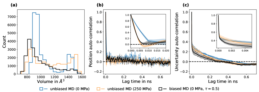
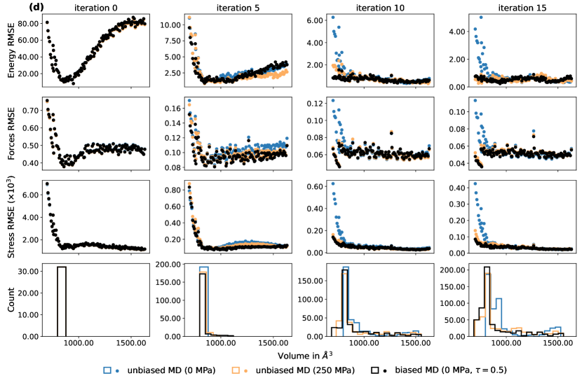
Figure 6: Evaluation of configurational space exploration rates using biased and unbiased MD simulations for MIL-53(Al). Here, MD simulations generate candidate pools of atomic configurations for AL algorithms. Results are provided for the posterior-based uncertainty quantification derived from sketched gradient features. Unlike unbiased MD simulations, which rely on atom-based uncertainties to terminate MD simulations, biased MD simulations use both total and atom-based uncertainties for biasing MD simulations and prompting their termination, respectively. We use three metrics to asses the exploration rates: (a) Volume distribution of configurations sampled throughout the experiment; (b) Auto-correlation functions for positions; and (c) Auto-correlation functions for atom-based uncertainties. Shaded areas denote the standard deviation across three independent runs. (d) Time evolution of the volume distribution of configurations acquired during training and of energy, force, and stress RMSEs evaluated on the test data set depending on the unit cell volume. Bias-stress-driven MD simulations achieve exploration rates comparable to those of high-pressure unbiased MD simulations. They efficiently reduce RMSEs uniformly across the entire volume space, even in the early stages of AL, surpassing the performance of unbiased simulations.

Figure 6 assesses the extent to which uncertainty-biased (bias stress) MD simulations enhance the exploration of the extensive volume space of MIL-53(Al). In Fig. 6 (a), we observe a higher frequency of transitions between stable states for biased MD simulations than for zero-pressure MD counterparts. Additionally, uncertainty-biased simulations favor the exploration of smaller MIL-53(Al) volumes, in line with the results shown in Fig. 5. Figures 6 (b) and (c) present ACFs for both positions and uncertainty spaces, with estimated ACTs provided in Table 2. These results indicate that bias-stress-driven MD is at least as efficient as high-pressure MD simulations in exploring both spaces. Similar to alanine dipeptide, a faster decay of ACFs corresponds to smaller ACTs, indicating a faster exploration of the respective space.

Figure 6 (d) demonstrates the time evolution of energy, force, and stress RMSEs and reveals that local atomic environments in the large-pore state are effectively represented by those in the closed-pore state, explaining the stronger preference for smaller volumes as observed in Figure 6 (a) and Figures 5 (d) and (e). This effect is evident from the low force and stress RMSEs in the early iterations for the large-pore state, even though this state has not been explored yet. Furthermore, uncertainty-biased simulations consistently outperform their counterparts, starting from the early stages, by uniformly reducing errors across the test volume space.

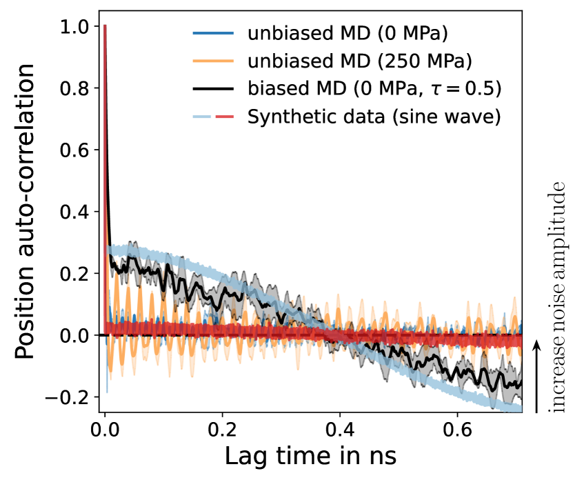
Figure 7: ACF for positions obtained by running biased and unbiased MD simulations at 300 K for MIL-53(Al). Shaded areas denote the standard deviation across three independent runs. We employ a temperature of 300 K to reduce the probability of exploring the large-pore state of MIL-53(Al). The ACF exhibits strongly correlated motions attributed to volume fluctuations induced by the bias stress. These fluctuations can be modeled by a sine wave with a period twice the length of the simulation. The red line denotes a sine wave with a larger noise amplitude than the one denoted by the blue line.

From these results and the findings in Fig. 5 (d), we conclude that bias-stress-driven MD simulations significantly enhance the exploration of the relevant configurational space, including rare events (i.e., transitions between stable phases). However, in Table 2, we obtained longer ACTs for biased dynamics at 300 K compared to its unbiased counterparts, which seems to contradict our previous arguments. When examining the ACF shown in Fig. 7, it becomes evident that a stronger correlation in the position space results from the volume fluctuations induced in MIL-53(Al) by the bias stress. These fluctuations can be represented by a sine wave with additive random noise and a period twice the simulation’s length; see Methods. This observation implies that bias stress induces correlated motions in the MIL-53(Al) system, causing it to expand and contract alternately for half of the simulation time. This phenomenon results in periodic exploration of both the boundaries of small and large volumes within the configurational space.

In contrast to the conventional approaches, including the bias-forces-driven MD simulations, which aim for uncorrelated random-walk-like behavior of predetermined CVs to capture configurational changes, our method introduces correlated motion that explores the entire configurational space without prior knowledge. Increasing the amplitude of random noise in the sine wave reduces the amplitude of these fluctuations in the ACF, similar to raising the temperature in an atomic system. This decrease in the amplitude explains why this effect is not observed in Fig. 6 (b).

Discussion

Our present study investigates a new paradigm for data set generation, facilitating the development of high-quality MLIPs for chemically complex atomic systems. We employ uncertainty-biased MD simulations to generate candidate pools for AL algorithms. Our results show, for the first time, that applying uncertainty bias facilitates simultaneous exploration of extrapolative regions and rare events. Efficient exploration of both is crucial in constructing comprehensive training datasets, consequently enabling the development of uniformly accurate MLIPs. In contrast, classical enhanced sampling techniques (e.g., metadynamics) or unbiased MD simulations at elevated temperatures and pressures cannot simultaneously explore extrapolative regions and rare events. Enhanced sampling techniques were designed to ensure the reconstruction of the underlying Boltzmann distribution. However, this property is unnecessary for data set generation and limits their effectiveness in this context.

Furthermore, the performance of enhanced sampling techniques depends on the manual definition of hyper-parameters, e.g., CVs for metadynamics. Setting them requires expert knowledge because the wrong choice can limit the range of explored configurations. In contrast, uncertainty-biased MD simulations need to define an uncertainty threshold and biasing strength. Both parameters influence the exploration rate of configurational space without constraining the space that can be explored. The biasing strength is advantageous over defining transition temperatures and pressures as it reduces the risk of degrading the atomic system. Furthermore, employing species-dependent biasing strength can restrict biasing in sensitive configurational regions, e.g., biasing hydrogen atoms. Simultaneously, it enables targeted biasing of pre-defined atom groups similar to metadynamics.

We compare uncertainty quantification methods, including the variance of an ensemble of MLIPs, and ensemble-free methods derived from sketched gradient features, focusing on configurational space exploration rates and generating uniformly accurate potentials; see Supplementary Information. Overall, gradient-based approaches yield MLIPs with similar performance to those created using ensemble-based uncertainty while significantly reducing the computational cost of uncertainty quantification. For MIL-53(AL), we find that ensemble-based uncertainties overestimate the force error stronger than gradient-based approaches, resulting in earlier termination of MD simulations and potentially worse configurational space exploration. For alanine dipeptide, using an ensemble of MLIPs improves their robustness during MD simulations, facilitating CV space exploration. Therefore, improving the robustness of a single MLIP during an MD simulation is a promising research direction,[52] combined with the proposed ensemble-free techniques.

While this study thoroughly investigates AL with uncertainty-biased MD for generating candidate pools, further research is still necessary. For example, one should analyze how well uncertainty-biased MD explores a configurational space with multiple stable states and how it identifies the respective slow modes using solely uncertainty bias. Also, assessing the uniform accuracy of resulting MLIPs and the enhanced exploration in higher-dimensional CV spaces remains challenging. Although uncertainty-biased MD proves efficient, it comes with an additional computational cost, increasing the inference times by 1.3 to 1.7 compared to unbiased MD, mainly due to calculating uncertainty gradients. In cases with known CVs or transition conditions, this increase in the computational cost might exceed the benefits. Lastly, unlike MD, Monte Carlo simulations generally allow significant configurational changes, eliminating the need to explore intermediate transition paths. Combined with uncertainty bias, they might potentially avoid exploring intermediate, low-uncertainty transition regions, improving the efficiency of uncertainty-driven data generation.

Methods

Machine-learned interatomic potentials

We define an atomic configuration, $S=\{\mathbf{r}_{i},Z_{i}\}_{i=1}^{N_{\mathrm{at}}}$, where $\mathbf{r}_{i}\in\mathbb{R}^{3}$ are Cartesian coordinates and $Z_{i}\in\mathbb{N}$ is the atomic number of atom $i$, with a total of $N_{\mathrm{at}}$ atoms. Our focus lies on interatomic NN potentials, which map an atomic configuration to a scalar energy $E$. The mapping is denoted as $f_{\bm{\theta}}:S\mapsto E\in\mathbb{R}$, where $\bm{\theta}$ denotes the trainable parameters. By assuming the locality of interatomic interactions, we decompose the total energy of the system into individual atomic contributions[11]

$$E\left(S,\bm{\theta}\right)=\sum_{i=1}^{N_{\mathrm{at}}}E_{i}\left(S_{i},\bm{\theta}\right),$$ (1)

where $S_{i}$ is the local environment of atom $i$, defined by the cutoff radius $r_{\mathrm{c}}$. The trainable parameters $\bm{\theta}$ are learned from atomic data sets containing atomic configurations and their energies, atomic forces, and stress tensors.

Gradient-based uncertainties

We quantify the uncertainty of a trained MLIP by expanding its energy per atom $E_{\mathrm{at}}=E/N_{\mathrm{at}}$ around the locally optimal parameters $\bm{\theta}^{\ast}$[37, 38, 39]

$$E_{\mathrm{at}}\left(S,\bm{\theta}\right)\approx E_{\mathrm{at}}\left(S,\bm{\theta}^{\ast}\right)+\left(\bm{\theta}-\bm{\theta}^{\ast}\right)^{\top}\underbrace{\nabla_{\bm{\theta}}E_{\mathrm{at}}\left(S,\bm{\theta}\right)\Big{|}_{\bm{\theta}=\bm{\theta}^{\ast}}}_{=\phi\left(S\right)},$$ (2)

where $S$ denotes an atomic configuration as defined in the previous section. Gradient features $\phi\left(S\right)\in\mathbb{R}^{N_{\mathrm{feat}}}$ can be interpreted as the sensitivity of the energy to small perturbations of the parameters. Here, $N_{\mathrm{feat}}$ is the number of trainable parameters of the MLIP, and $N_{\mathrm{at}}$ is the number of atoms. We employ the energy per atom $E_{\mathrm{at}}$ in Eq. (2), as it accounts for the extensive nature of the energy that scales proportionally with the system size. This choice ensures that uncertainties defined using gradient features do not favor the selection of larger structures. Gradient features can also be expressed as the mean of their atomic contributions: $\phi=\sum_{i=1}^{N_{\mathrm{at}}}\phi_{i}/N_{\mathrm{at}}$. For atomic gradient features $\phi_{i}$, using the energy per atom in Eq. (2) is unnecessary. Here, we use $\phi=\phi\left(S\right)$ and $\phi_{i}=\phi_{i}\left(S_{i}\right)$, with $S_{i}$ denoting the local environment of an atom $i$, to simplify the notation. Thus, gradient features can be used to quantify uncertainties in total and atom-based properties of an atomic system, such as energy and atomic forces, respectively.

Particularly, we define the atom-based model’s uncertainty (atomic forces) by employing squared distances between atomic gradient features

$$u_{i}^{2}=\min_{\phi_{j}^{\prime}\in\Phi_{\mathrm{train}}}\Big{\lVert}\left(\phi_{i}-\phi_{j}^{\prime}\right)\Big{\rVert}_{2}^{2}.$$ (3)

Alternatively, we consider Bayesian linear regression in Eq. (2) and compute the posterior uncertainty as

$$u_{i}^{2}=\lambda^{2}\phi_{i}^{\top}\left(\Phi_{\mathrm{train}}^{\top}\Phi_{\mathrm{train}}+\lambda^{2}\mathbf{I}\right)^{-1}\phi_{i},$$ (4)

where $\lambda$ is the regularization strength. Here, we define $\Phi_{\mathrm{train}}=\phi_{i}\left(\mathcal{X}_{\mathrm{train}}\right)\in\mathbb{R}^{\left(N_{\mathrm{at}}\cdot N_{\mathrm{train}}\right)\times N_{\mathrm{feat}}}$ with $\mathcal{X}_{\mathrm{train}}$ denoting the local atomic environments of configurations in the training set of size $N_{\mathrm{train}}$. In this work, we refer to our uncertainties as distance- and posterior-based uncertainties. Equivalent results can be obtained for total uncertainties (energy), employing gradient features $\phi=\sum_{i=1}^{N_{\mathrm{at}}}\phi_{i}/N_{\mathrm{at}}$ with $\Phi_{\mathrm{train}}=\phi\left(\mathcal{X}_{\mathrm{train}}\right)\in\mathbb{R}^{N_{\mathrm{train}}\times N_{\mathrm{feat}}}$.

Calculating uncertainties using gradient features is computationally challenging, especially for the posterior-based approach, for which a single uncertainty evaluation scales as $\mathcal{O}\left(N_{\mathrm{feat}}^{2}\right)$. Therefore, we employ the sketching technique[40] to reduce the dimensionality of gradient features, i.e., $\phi_{i}^{\mathrm{rp}}=\mathbf{U}\phi_{i}\in\mathbb{R}^{N_{\mathrm{rp}}}$ with $N_{\mathrm{rp}}$ and $\mathbf{U}\in\mathbb{R}^{N_{\mathrm{rp}}\times N_{\mathrm{feat}}}$ denoting the number of random projections and a random matrix, respectively.[38, 39] In previous work,[38] we have observed that uncertainties derived from sketched gradient features demonstrate a better correlation with RMSEs of related properties than those based on last-layer features.[53, 37, 54] More details on sketched gradient features can be found in the following sections. Atom-based uncertainties, defined by the distances between gradient features, scale linearly with both the system size and the number of training structures, i.e., as $\mathcal{O}\left(N_{\mathrm{at}}N_{\mathrm{train}}\right)$. Consequently, they require an additional approximation to ensure computational efficiency. To address this, we employed the batch selection algorithm that maximizes distances within the training set, allowing us to identify the most representative subset of atomic gradient features; see the following sections.

Uncertainty-biased molecular dynamics

Following previous works,[33, 34] we define a biased energy as

$$E^{\mathrm{biased}}\left(S,\bm{\theta}\right)=E\left(S,\bm{\theta}\right)-\tau u\left(S,\bm{\theta}\right),$$ (5)

where $\tau$ denotes the biasing strength. The negative sign ensures that negative uncertainty gradients with respect to atomic positions (bias forces) drive the system toward high uncertainty regions; see Fig. 1 (c). In this work, we use AD to compute bias forces acting on atom $i$, denoted as $-\nabla_{\mathbf{r}_{i}}u\left(S,\bm{\theta}\right)$ with atomic positions $\mathbf{r}_{i}$. The total biased force on atom $i$ reads

$$\mathbf{F}_{i}^{\mathrm{biased}}\left(S,\bm{\theta}\right)=\mathbf{F}_{i}\left(S,\bm{\theta}\right)+\tau\nabla_{\mathbf{r}_{i}}u\left(S,\bm{\theta}\right).$$ (6)

These biased forces can be used for MD simulations in, e.g., canonical ($NVT$) statistical ensemble to bias the exploration of the configurational space.

In the case of bulk atomic systems, the configurational space often includes variations in cell parameters, which define the shape and size of the unit cell, necessitating enhanced exploration of them. For this purpose, we propose the concept of bias stress, defined by

$$\frac{1}{V}\left.\nabla_{\bm{\epsilon}}u\left(S,\bm{\theta}\right)\right|_{\bm{\epsilon}=\mathbf{0}}$$

with $V$ denoting the volume of the periodic cell. This expression is motivated by the definition of the stress tensor.[55] Here, $u\left(S,\bm{\theta}\right)$ denotes the uncertainty after a strain deformation of the bulk atomic system with the symmetric tensor $\bm{\epsilon}\in\mathbb{R}^{3\times 3}$, i.e., $\tilde{\mathbf{r}}=\left(\mathbf{1}+\bm{\epsilon}\right)\cdot\mathbf{r}$. The calculation of the bias stress is straightforward with AD. The total biased stress reads

$$\bm{\sigma}^{\mathrm{biased}}\left(S,\bm{\theta}\right)=\bm{\sigma}\left(S,\bm{\theta}\right)-\tau\frac{1}{V}\left.\nabla_{\bm{\epsilon}}u\left(S,\bm{\theta}\right)\right|_{\bm{\epsilon}=\mathbf{0}}.$$ (7)

The bias stress tensor in Eq. (7) effectively reduces the internal pressure in the bulk atomic system. We propose combining the bias stress tensor with MD simulations conducted under constant pressure conditions ($NpT$ statistical ensemble) to enhance the data-driven exploration of cell parameters and pressure-induced transitions in bulk materials.

Uncertainty gradients exhibit different magnitudes compared to energy gradients. Thus, re-scaling uncertainty gradients is necessary to ensure consistent driving toward uncertain regions. Building upon the approach introduced in Ref. 34, we implement a re-scaling technique that monitors the magnitudes of both actual and bias forces (alternatively, actual and bias stresses) over $N$ steps and then computes the ratio between them. To re-scale bias forces, we use the following expression

$$\tau_{t}=\tau_{0}\times\frac{\sqrt{\sum_{n=0}^{N-1}\lVert\mathbf{F}_{t-n\Delta t}\rVert_{2}^{2}}}{\sqrt{\sum_{n=0}^{N-1}\lVert\nabla_{\mathbf{r}_{i}}u_{t-n\Delta t}\rVert_{2}^{2}}}.$$ (8)

An equivalent expression is applied for bias stresses.

The re-scaling of uncertainty gradients is reminiscent of the AdaGrad algorithm,[56] which dynamically adjusts the learning rate (analogous to the biasing strength) based on historical gradients from previous iterations. While incorporating momentum through exponential moving averages can improve the AdaGrad approach, treating all past gradients with equal weight is essential within the context of this study. Our attempts to damp learning along directions with high curvature (high-frequency oscillations), similar to the Adam optimizer,[57] did not yield improved performance. We further find that employing species-dependent biasing strengths for bias forces, $\tau\rightarrow\tau_{Z_{i}}$, with a particular emphasis on damping biasing of hydrogen atoms, improves the efficiency of biased MD simulations.

We employ biased MD simulation to generate a candidate pool for AL, as depicted in Fig. 1 (a). To further enhance the exploration of the relevant configurational space and improve the computational efficiency of AL, we employ multiple parallel MD simulations. We expect biased MD simulations to have relatively short auto-correlation times obtained from position and uncertainty auto-correlation functions. Short auto-correlation times imply that the generated candidates will be less correlated than those generated with unbiased MD simulations. However, we cannot guarantee the generation of uncorrelated samples with biased MD simulations throughout AL, particularly in later AL iterations when the uncertainty level is reduced. Therefore, we propose to use batch selection algorithms (see later sections) that select $N_{\mathrm{batch}}>1$ samples at once. These algorithms enforce the informativeness and diversity of the selected atomic configurations and the resulting training data set.

Gaussian moment neural network

This work uses the Gaussian moment neural network (GM-NN) approach for modeling interatomic interactions.[15, 17] GM-NN employs an artificial NN to map a local atomic environment $S_{i}$ to the atomic energy $E_{i}\left(S_{i},\bm{\theta}\right)$; see Eq. (1). It uses a fully-connected feed-forward NN with two hidden layers[15, 17]

$$\begin{split}y_{i}&=0.1\cdot\mathbf{b}^{(3)}+\frac{1}{\sqrt{d_{2}}}\mathbf{W}^{(3)}\phi\left(0.1\cdot\mathbf{b}^{(2)}+\right.\\ &\quad\left.\frac{1}{\sqrt{d_{1}}}\mathbf{W}^{(2)}\phi\left(0.1\cdot\mathbf{b}^{(1)}+\frac{1}{\sqrt{d_{0}}}\mathbf{W}^{(1)}\mathbf{G}_{i}\right)\right),\end{split}$$ (9)

with $\mathbf{W}^{(l+1)}\in\mathbb{R}^{d_{l+1}\times d_{l}}$ and $\mathbf{b}^{(l+1)}\in\mathbb{R}^{d_{l+1}}$ representing the weights and biases of layer $l+1$. In this work, we employ a NN with $d_{0}=910$ input neurons (corresponding to the dimension of the input feature vector $\mathbf{G}_{i}=\mathbf{G}_{i}\left(S_{i}\right)$), $d_{1}=d_{2}=512$ hidden neurons, and a single output neuron, $d_{3}=1$. The network’s weights $\mathbf{W}^{(l+1)}$ are initialized by selecting entries from a normal distribution with zero mean and unit variance. The trainable bias vectors $\mathbf{b}^{(l+1)}$ are initialized to zero. To improve the accuracy and convergence of the GM-NN model, we implement a neural tangent parameterization (factors of $0.1$ and $1/\sqrt{d_{l}}$).[58] For the activation function $\phi$, we use the Swish/SiLU function.[59, 60]

To aid the training process, we scale and shift the output of the NN

$$E_{i}\left(S_{i},\bm{\theta}\right)=c\cdot(\rho_{Z_{i}}y_{i}+\mu_{Z_{i}}),$$ (10)

where the trainable shift parameters $\mu_{Z_{i}}$ are initialized by solving a linear regression problem, and the trainable scale parameters $\rho_{Z_{i}}$ are initialized to one. The per-atom RMSE of the regression solution determines the constant $c$.[17]

GM-NN models employ a Gaussian moment (GM) representation to encode the invariance of total energy with respect to translations, rotations, and permutations of the same species.[15] By computing pairwise distance vectors $\mathbf{r}_{ij}=\mathbf{r}_{i}-\mathbf{r}_{j}$ and then splitting them into radial and angular components, denoted as $r_{ij}=\lVert\mathbf{r}_{ij}\rVert_{2}$ and $\hat{\mathbf{r}}_{ij}=\mathbf{r}_{ij}/r_{ij}$, respectively, we obtain GMs as follows

$$\bm{\Psi}_{i,L,s}=\sum_{j\neq i}R_{Z_{i},Z_{j},s}\left(r_{ij},\bm{\beta}\right)\hat{\mathbf{r}}_{ij}^{\otimes L},$$ (11)

where $\hat{\mathbf{r}}_{ij}^{\otimes L}=\hat{\mathbf{r}}_{ij}\otimes\cdots\otimes\hat{\mathbf{r}}_{ij}$ is the $L$-fold outer product. The nonlinear radial functions $R_{Z_{i},Z_{j},s}\left(r_{ij},\bm{\beta}\right)$ are defined as a sum of Gaussian functions $\Phi_{s^{\prime}}\left(r_{ij}\right)$ ($N_{\mathrm{Gauss}}=9$ for this work)[17]

$$R_{Z_{i},Z_{j},s}\left(r_{ij},\bm{\beta}\right)=\frac{1}{\sqrt{N_{\mathrm{Gauss}}}}\sum_{s^{\prime}=1}^{N_{\mathrm{Gauss}}}\beta_{Z_{i},Z_{j},s,s^{\prime}}\Phi_{s^{\prime}}\left(r_{ij}\right).$$ (12)

The factor $1/\sqrt{N_{\mathrm{Gauss}}}$ impacts the effective learning rate inspired by neural tangent parameterization.[58] The radial functions are centered at equidistantly spaced grid points ranging from $r_{\mathrm{min}}=0.5$ Å to $r_{\mathrm{c}}$, set to 5.0 Å and 6.0 Å for alanine dipeptide and MIL-53(Al), respectively. The radial functions are re-scaled by a cosine cutoff function,[11] to ensure a smooth dependence on the number of atoms within the cutoff sphere. Chemical information is embedded in the GM representation through trainable parameters $\beta_{Z_{i},Z_{j},s,s^{\prime}}$, with the index $s$ iterating over the number of independent radial basis functions ($N_{\mathrm{basis}}=7$ for this work).

Features invariant to rotations, $\mathbf{G}_{i}$, are obtained by computing full tensor contractions of tensors defined in Eq. (11), e.g.,[15, 17]

$$G_{i,s_{1},s_{2},s_{3}}=\left(\bm{\Psi}_{i,1,s_{1}}\right)_{a}\left(\bm{\Psi}_{i,1,s_{2}}\right)_{b}\left(\bm{\Psi}_{i,2,s_{3}}\right)_{a,b},$$ (13)

where we use Einstein notation, i.e., the right-hand sides are summed over $a,b\in\{1,2,3\}$. Specific full tensor contractions are defined by using generating graphs.[61] In a practical implementation, we compute all GMs at once and reduce the number of invariant features based on the permutational symmetries of the respective graphs.

All parameters $\bm{\theta}=\{\mathbf{W},\textbf{b},\bm{\beta},\bm{\rho},\bm{\mu}\}$ of the NN are optimized by minimizing the combined squared loss on training data $\mathcal{D}_{\mathrm{train}}=\left(\mathcal{X}_{\mathrm{train}},\mathcal{Y}_{\mathrm{train}}\right)$, with $\mathcal{X}_{\mathrm{train}}=\{S^{(k)}\}_{k=1}^{N_{\mathrm{train}}}$ and $\mathcal{Y}_{\mathrm{train}}=\{E_{k}^{\mathrm{ref}},\{\mathbf{F}_{i,k}^{\mathrm{ref}}\}_{i=1}^{N_{\mathrm{at}}},\bm{\sigma}_{k}^{\mathrm{ref}}\}_{k=1}^{N_{\mathrm{train}}}$,

$$\begin{split}\mathcal{L}\left(\bm{\theta},\mathcal{D}_{\mathrm{train}}\right)=\sum_{k=1}^{N_{\mathrm{train}}}\Bigg{[}C_{\mathrm{e}}&\Big{\lVert}E_{k}^{\mathrm{ref}}-E(S^{(k)},\bm{\theta})\Big{\rVert}_{2}^{2}+\\ C_{\mathrm{f}}\sum_{i=1}^{N_{\mathrm{at}}^{(k)}}&\Big{\lVert}\mathbf{F}_{i,k}^{\mathrm{ref}}-\mathbf{F}_{i}\left(S^{(k)},\bm{\theta}\right)\Big{\rVert}_{2}^{2}+\\ C_{\mathrm{s}}&\Big{\lVert}V_{k}\bm{\sigma}_{k}^{\mathrm{ref}}-V_{k}\bm{\sigma}\left(S^{(k)},\bm{\theta}\right)\Big{\rVert}_{2}^{2}\Bigg{]}.\end{split}$$ (14)

We have chosen $C_{\mathrm{e}}=1.0$, $C_{\mathrm{f}}=4.0\leavevmode\nobreak\ \text{\AA}^{2}$, and $C_{\mathrm{s}}=0.01$ to balance the relative contributions of energies, forces, and stresses, respectively.

Using AD, we compute atomic forces as negative gradients of total energy with respect to atomic coordinates

$$\mathbf{F}_{i}\left(S^{(k)},\bm{\theta}\right)=-\nabla_{\mathbf{r}_{i}}E\left(S^{(k)},\bm{\theta}\right).$$ (15)

Furthermore, we use AD to compute stress tensor, defined by[55]

$$\bm{\sigma}\left(S^{(k)},\bm{\theta}\right)=\frac{1}{V_{k}}\left.\nabla_{\bm{\epsilon}}E\left(S^{(k)},\bm{\theta}\right)\right|_{\bm{\epsilon}=\mathbf{0}},$$ (16)

where $E\left(S^{(k)},\bm{\theta}\right)$ is total energy after a strain deformation with symmetric tensor $\bm{\epsilon}\in\mathbb{R}^{3\times 3}$, i.e., $\tilde{\mathbf{r}}=\left(\mathbf{1}+\bm{\epsilon}\right)\cdot\mathbf{r}$. As the stress tensor is symmetric, we use only its upper triangular part in the loss function. Here, $V_{k}$ is the volume of the periodic cell.

We employ the Adam optimizer[57] to minimize the loss function. The respective parameters of the optimizer are $\beta_{1}=0.9$, $\beta_{2}=0.999$, and $\epsilon=10^{-7}$. Usually, we work with a mini-batch of 32 molecules. However, smaller mini-batches were used in the initial AL iterations because the training data sizes were less than 32. The layer-wise learning rates are decayed linearly. The initial values are set to 0.03 for the parameters of the fully connected layers, 0.02 for the trainable representation, as well as 0.05 and 0.001 for the shift and scale parameters of atomic energies, respectively. The training is performed for 1000 training epochs. To prevent overfitting during training, we employ the early stopping technique.[62] All models are trained using PyTorch.[45]

Sketched gradient features

We obtain atomic gradient features by computing gradients of Eq. (1) with respect to the parameters of the fully connected layers in Eq. (9). Particularly, we make use of the product structure of atomic gradient features. To obtain the latter, we re-write the network in Eq. (9) as follows

$$\begin{split}&\mathbf{z}_{i}^{(l+1)}=\tilde{\mathbf{W}}^{(l+1)}\tilde{\mathbf{x}}_{i}^{(l)}\in\mathbb{R}^{d_{l+1}},\\ &\tilde{\mathbf{W}}^{(l+1)}=\left(\mathbf{W}^{(l+1)},\mathbf{b}^{(l+1)}\right)\in\mathbb{R}^{d_{l+1}\times\left(d_{l}+1\right)},\\ &\tilde{\mathbf{x}}_{i}^{(l)}=\left(\frac{1}{\sqrt{d_{l}}}\mathbf{x}_{i}^{(l)},0.1\right)^{\top}\in\mathbb{R}^{d_{l}},\end{split}$$ (17)

where $\mathbf{z}^{(l)}$ and $\mathbf{x}^{(l)}$ denote the pre- and post-activation vectors of layer $l$. Thus, atomic gradient features read

$$\begin{split}\phi_{i}(S_{i})&=\left(\frac{\partial\mathbf{z}_{i}^{(L)}}{\partial\tilde{\mathbf{W}}^{(1)}},\cdots,\frac{\partial\mathbf{z}_{i}^{(L)}}{\partial\tilde{\mathbf{W}}^{(L)}}\right)\\ &=\left(\frac{\partial\mathbf{z}_{i}^{(L)}}{\partial\mathbf{z}_{i}^{(1)}}\otimes\tilde{\mathbf{x}}_{i}^{(0)},\cdots,\frac{\partial\mathbf{z}_{i}^{(L)}}{\partial\mathbf{z}_{i}^{(L)}}\otimes\tilde{\mathbf{x}}_{i}^{(L-1)}\right).\end{split}$$ (18)

To make the calculation of gradient features computationally tractable, we employ the random projections (sketching) technique,[40] as proposed in Refs. 39, 38. For atomic gradient features $\phi_{i}\left(S_{i}\right)\in\mathbf{R}^{N_{\mathrm{feat}}}$ and a random matrix $\mathbf{U}\in\mathbb{R}^{N_{\mathrm{rp}}\times N_{\mathrm{feat}}}$—with $N_{\mathrm{feat}}$ and $N_{\mathrm{rp}}$ representing the number of atomic features and random projections, respectively—we can define randomly projected atomic gradient features as

$$\phi_{i}^{\mathrm{rp}}\left(S_{i}\right)=\mathbf{U}\phi_{i}\left(S_{i}\right)\in\mathbb{R}^{N_{\mathrm{rp}}}.$$ (19)

While a Gaussian sketch could be employed, where the elements of $\mathbf{U}$ are drawn from standard normal distributions, we use a tensor sketching approach that is more runtime and memory efficient.[39] Specifically, denoting the element-wise or Hadamard product as $\odot$, we compute

$$\phi_{i}^{\mathrm{rp}}(S_{i})=\sum_{l=1}^{L}\left(\mathbf{U}_{\mathrm{out}}^{(l)}\phi_{i,\mathrm{out}}^{(l)}(S_{i})\right)\odot\left(\mathbf{U}_{\mathrm{in}}^{(l-1)}\phi_{i,\mathrm{in}}^{(l-1)}(S_{i})\right),$$ (20)

with $\phi_{i,\mathrm{out}}^{(l)}(S_{i})=\partial\mathbf{z}_{i}^{(L)}/\partial\mathbf{z}_{i}^{(l)}$ and $\phi_{i,\mathrm{in}}^{(l)}(S_{i})=\tilde{\mathbf{x}}_{i}^{(l)}$. All entries of $\mathbf{U}_{\mathrm{in}}^{(l)}$ and $\mathbf{U}_{\mathrm{out}}^{(l)}$ are sampled independently from a standard normal distribution.

For atom-based uncertainties, we can directly use the sketched atomic gradient features. For (total) uncertainties per atom, we need to work with a mean $\phi(S)=\sum_{i=1}^{N_{\mathrm{at}}}\phi_{i}(S_{i})/N_{\mathrm{at}}$. Thus, we use that the individual projections (rows of Eq. (20)) are linear in the features and obtain for the (total) gradient features[38]

$$\phi^{\mathrm{rp}}(S)=\frac{1}{N_{\mathrm{at}}}\sum_{i=1}^{N_{\mathrm{at}}}\sum_{l=1}^{L}\left(\mathbf{U}_{\mathrm{out}}^{(l)}\phi_{i,\mathrm{out}}^{(l)}(S_{i})\right)\odot\left(\mathbf{U}_{\mathrm{in}}^{(l-1)}\phi_{i,\mathrm{in}}^{(l-1)}(S_{i})\right),$$ (21)

given that all of the individual random projections use the same random matrices.

Ensemble-based uncertainty quantification

The variance of the predictions of individual models in an ensemble of MLIPs can be used to quantify their uncertainty. Thus, we define the variance of predicted energy as

$$u^{2}=\frac{1}{M}\sum_{j=1}^{M}\lVert E_{j}-\bar{E}\rVert_{2}^{2},$$ (22)

where $M$ is the number of models in the ensemble. The variance of atomic forces reads

$$u_{i}^{2}=\frac{1}{3M}\sum_{j=1}^{M}\lVert\mathbf{F}_{i,j}-\bar{\mathbf{F}}_{i}\rVert_{2}^{2},$$ (23)

Here, $\bar{E}$ and $\bar{\mathbf{F}}_{i}$ denote the arithmetic mean of the predictions from individual models. Our experiments demonstrated that $M=3$ is sufficient to obtain good performance. Using larger ensembles would make the ensemble-based uncertainty quantification even more computationally inefficient than gradient-based alternatives.

Batch selection methods

The simplest batch selection method is based on querying points only by their uncertainty values. Specifically, given the already selected structures $\mathcal{X}_{\mathrm{batch}}$ from an unlabeled pool $\mathcal{X}_{\mathrm{pool}}$ we select the next point by

$$S=\underset{S\in\mathcal{X}_{\mathrm{pool}}\backslash\mathcal{X}_{\mathrm{batch}}}{\operatorname*{arg\,max}}\,u\left(S\right),$$ (24)

until $N_{\mathrm{batch}}>1$ structures are selected. In this work, we use this selection method combined with ensemble-based uncertainties.

For the posterior-based uncertainty, we can constrain the diversity of the selected batch by using the posterior covariance between structures

$$\mathrm{Cov}\left(S,S^{\prime}\right)=\lambda^{2}\phi\left(S\right)^{\top}\left(\Phi_{\mathrm{train}}^{\top}\Phi_{\mathrm{train}}+\lambda^{2}\mathbf{I}\right)^{-1}\phi\left(S^{\prime}\right),$$ (25)

with $\Phi_{\mathrm{train}}=\phi\left(\mathcal{X}_{\mathrm{train}}\right)$. The corresponding method greedily selects structures, i.e., one structure per iteration, such that the determinant of the covariance matrix is maximized[63, 38, 39]

$$\begin{split}&S=\\ &\underset{S\in\mathcal{X}_{\mathrm{pool}}\backslash\mathcal{X}_{\mathrm{batch}}}{\operatorname*{arg\,max}}\,\det\left[\mathrm{Cov}\left(\mathcal{X}_{\mathrm{batch}}\cup\{S\},\mathcal{X}_{\mathrm{batch}}\cup\{S\}\right)\right].\end{split}$$ (26)

For the distance-based uncertainty, we ensure the diversity of the acquired batch by greedily selecting structures with a maximum distance to all previously selected and training data points. The respective selection method reads[64, 38, 39]

$$\begin{split}&S=\\ &\underset{S\in\mathcal{X}_{\mathrm{pool}}\backslash\mathcal{X}_{\mathrm{batch}}}{\operatorname*{arg\,max}}\,\underset{S^{\prime}\in\mathcal{X}_{\mathrm{train}}\cup\mathcal{X}_{\mathrm{batch}}}{\min}\,\Big{\lVert}\phi\left(S\right)-\phi\left(S^{\prime}\right)\Big{\rVert}_{2}^{2}.\end{split}$$ (27)

We also applied this batch selection method to define the most representative subset of atomic gradient features when calculating atom-based uncertainty using feature space distances.

Conformal prediction

Conformal prediction methods offer distribution-free uncertainty quantification with guaranteed finite sample coverage,[65, 66, 67, 68, 69] thus ensuring calibration. Finite sample coverage can be defined as

$$\mathbb{P}\{y_{\mathrm{test}}\in C\left(x_{\mathrm{test}}\right)\}\geq 1-\alpha.$$ (28)

Here, $\left(x_{\mathrm{test}},y_{\mathrm{test}}\right)$ are the newly observed data, while $C$ defines the prediction set based on previous observations $\{\left(x_{k},y_{k}\right)\}_{k=1}^{N_{\mathrm{calibr}}}$. The user determines the hyper-parameter $\alpha$ and defines the desired confidence level. CP methods guarantee that the prediction set contains the true label with a probability of almost $1-\alpha$.

We employ inductive CP, which comprises the following steps:[65, 69] (1) A subset of calibration data, sized $N_{\mathrm{calibr}}$, is selected, and the corresponding errors are computed on this subset. For atomic forces, we employ RMSEs $\Delta\mathbf{F}_{i}^{2}=\lVert\mathbf{F}_{i}-\mathbf{F}_{i}^{\mathrm{ref}}\rVert_{2}^{2}/3$, while for total energies the respective energy absolute errors per atom, $\Delta e=\lvert E-E^{\mathrm{ref}}\rvert/N_{\mathrm{at}}$, are used. (2) The uncertainty $u\left(S\right)$ is calculated for this subset of data. (3) The ratio $\Delta e/u\left(S\right)$ or $\Delta\mathbf{F}_{i}/u\left(S_{i}\right)$ is computed. (4) Utilizing quantile regression, the $\left(1-\alpha\right)\left(N_{\mathrm{calibr}}+1\right)/N_{\mathrm{calibr}}$-th quantile, denoted as $s$, is determined. (5) This $s$ value is applied to new observations, resulting in the re-scaled and calibrated uncertainty, $\tilde{u}=s\cdot u$.

Test data for alanine dipeptide

The test data set for alanine dipeptide comprises 2000 configurations randomly selected from an MD trajectory. This trajectory was generated within the ASE simulation package[46] by running an MD simulation in the canonical ($NVT$) statistical ensemble using the Langevin thermostat at $T=1200$ K. We have used a time step of 0.5 fs and a total simulation time of 1 ns. The AMBER ff19SB force field has provided forces,[43] as implemented in the TorchMD package using PyTorch.[44, 45] The data set effectively covers the relevant configurational space of alanine dipeptide, representing an upper boundary in exploring its CVs.

Coverage of collective variable space

To measure how well different methods explore the (bounded) space of interest, we implement a tree-based weighted recursive partitioning of a $d$-dimensional Euclidean space, which is reminiscent of quadtrees [70] and matrix-based octrees [71] but allows to choose how many times $n$ to split each dimension. Thus, the variety of the tree is $k=n^{d}$. Each node of this complete k-ary tree encodes a generalized hypercube of $d$ dimensions, where each side length depends on the boundaries of the original space. The root node represents the full bounded space. A tree of height $L$ has total number of partitions equal to $(k^{L+1}-1)/(k-1)$, and each level $\ell$ has $k^{\ell}$ nodes. The hyper-parameters we choose in this paper are $n=2$, $d=2$ (for the CVs $\phi$ and $\psi$ of alanine dipeptide), and $L=5$, for a total of $1365$ partitions of the space of interest.

Our proposed surface coverage metric uses this data structure as a proxy to capture how many space partitions a method can explore in the least amount of iterations. At the same time, we need to penalize methods that get stuck in a region of the space, exploring partitions of smaller volumes, that is, those represented by nodes at deeper levels in the tree. For this reason, each node at level $\ell$ is associated with a reward (or weight) of $1/k^{\ell}$, so each level of the tree has a cumulative reward of $1$. The optimal strategy would be to perform a breadth-first search of the nodes of this tree, which translates into observing the largest partitions of unobserved space first. In addition, partitions that are revisited by the methods give no additional reward, so there is no gain in getting stuck in a certain partition. We visually represent the idea of the algorithm in the Supplementary Information for the simple case of $d=2$.

Auto-correlation analysis

We evaluate the performance of uncertainty-biased MD simulations by investigating the auto-correlation between subsequent time frames of the MD trajectory. The auto-correlation function (ACF) is defined as[72]

$$A_{\mathcal{O}}\left(k\right)=\frac{\langle\mathcal{O}_{i}\mathcal{O}_{i+k}\rangle-\langle\mathcal{O}_{i}\rangle^{2}}{\langle\mathcal{O}_{i}^{2}\rangle-\langle\mathcal{O}_{i}\rangle^{2}},$$ (29)

where $\langle\cdots\rangle$ denotes the thermodynamic expectation value, $k$ is the lag time, and $\mathcal{O}$ is an observable, e.g., atomic forces or atom-based uncertainties. From ACF, we can calculate the auto-correlation time (ACT) for an MD trajectory of length $N$

$$\mathrm{ACT}_{\mathcal{O}}=\frac{1}{2}+\sum_{k=1}^{N}A_{\mathcal{O}}\left(k\right)\left(1-\frac{k}{N}\right).$$ (30)

ACT is related to effective sample size (ESS) by

$$\mathrm{ESS}_{\mathcal{O}}=\frac{N}{2\cdot\mathrm{ACT}_{\mathcal{O}}}.$$ (31)

In this work, we calculate ESS as implemented in TensorFlow[73] and use it to estimate the ACT.

Density functional theory calculations

DFT calculations for MIL-53(Al) were performed using the CP2K simulation package (version 2023.1).[47] To ensure consistency with incremental learning experiments,[32] we employed the PBE functional[48] with Grimme D3 dispersion correction.[49] A hybrid basis set, combining TZVP Gaussian basis functions and plane waves, was employed.[74] GTH pseudopotentials were used to smoothen the electron density near the nuclei.[75] To ensure the convergence of force and stress calculations, a plane wave cutoff energy of 1000 Ry was selected.

Random perturbation of atomic configurations

In this work, we obtain randomly perturbed atomic configurations by adding atomic shifts, denoted as $\bm{\delta}_{i}$, to the original atomic positions $\mathbf{r}_{i}$

$$\tilde{\mathbf{r}}_{i}=\mathbf{r}_{i}+\bm{\delta}_{i}.$$ (32)

The components of $\bm{\delta}_{i}$ are sampled independently from a uniform distribution: for alanine dipeptide, the range is between $-0.02$ Å and $0.02$ Å, and for MIL-53(Al), it is between $-0.08$ Å and $0.08$ Å. Additionally, for MIL-53(Al), we introduce random perturbations to its periodic cell $\mathbf{B}$ using a strain deformation $\bm{\epsilon}=\left(\mathbf{A}+\mathbf{A}^{\top}\right)/2$, where the components of $\mathbf{A}$ are sampled independently from a uniform distribution between $-0.02$ and $0.02$. This transformation can be expressed as

$$\tilde{\mathbf{B}}=\mathbf{B}\left(\mathbf{I}+2\bm{\epsilon}\right)^{1/2}.$$ (33)

The shifted atomic positions are re-scaled according to

$$\tilde{\tilde{\mathbf{r}}}_{i}=\left(\mathbf{I}+2\bm{\epsilon}\right)^{1/2}\tilde{\mathbf{r}}_{i}.$$ (34)

Sine wave with additive random noise

We model large-amplitude volume fluctuations in MIL-53(Al) induced by the bias stress using a sine wave with period $T_{0}$ and additive random noise $N\left(t\right)$

$$A\sin\left(\frac{2\pi t}{T_{0}}\right)+BN\left(t\right),$$

where $A$ and $B$ denote the amplitude of the sine wave and random noise, respectively. In this work, $N\left(t\right)\sim\mathcal{N}\left(0,1\right)$ represents random noise following a normal distribution with zero mean and unit variance. We chose $A=1.0$ and $B=0.5$ for the blue line in Fig. 7. For the red line, we increase the noise amplitude to $B=2.0$. To represent the volume fluctuations induced in MIL-53(Al) (see Fig. 7), a sine wave with the period twice the length of the MD simulation, i.e., $T_{0}=3.2$ ns is required.

Data Availability

The code, trained models, and generated data sets will be made publicly available upon publication.

Author contributions

All authors designed the project, discussed the results, and wrote the manuscript. V.Z. performed the calculations.

Additional information

Supplementary Information accompanies.

References

- [1] Butler, K. T., Davies, D. W., Cartwright, H., Isayev, O. & Walsh, A. Machine learning for molecular and materials science. \JournalTitleNature 559, 547–555, DOI: 10.1038/s41586-018-0337-2 (2018).
- [2] Xie, Y. et al. Uncertainty-aware molecular dynamics from bayesian active learning for phase transformations and thermal transport in sic. \JournalTitlenpj Comput. Mater. 9, 36, DOI: 10.1038/s41524-023-00988-8 (2023).
- [3] Gubaev, K. et al. Performance of two complementary machine-learned potentials in modelling chemically complex systems. \JournalTitlenpj Comput. Mater. 9, 129, DOI: 10.1038/s41524-023-01073-w (2023).
- [4] Langer, M. F., Goeßmann, A. & Rupp, M. Representations of molecules and materials for interpolation of quantum-mechanical simulations via machine learning. \JournalTitlenpj Comput. Mater. 8, 41, DOI: 10.1038/s41524-022-00721-x (2022).
- [5] Rupp, M., Tkatchenko, A., Müller, K.-R. & von Lilienfeld, O. A. Fast and Accurate Modeling of Molecular Atomization Energies with Machine Learning. \JournalTitlePhys. Rev. Lett. 108, 058301, DOI: 10.1103/PhysRevLett.108.058301 (2012).
- [6] Faber, F. A., Christensen, A. S., Huang, B. & von Lilienfeld, O. A. Alchemical and structural distribution based representation for universal quantum machine learning. \JournalTitleJ. Chem. Phys. 148, 241717, DOI: 10.1063/1.5020710 (2018).
- [7] Shapeev, A. V. Moment tensor potentials: A class of systematically improvable interatomic potentials. \JournalTitleMultiscale Model. Simul. 14, 1153–1173, DOI: 10.1137/15M1054183 (2016).
- [8] Drautz, R. Atomic cluster expansion for accurate and transferable interatomic potentials. \JournalTitlePhys. Rev. B 99, 014104 (2019).
- [9] Bartók, A. P., Payne, M. C., Kondor, R. & Csányi, G. Gaussian approximation potentials: The accuracy of quantum mechanics, without the electrons. \JournalTitlePhys. Rev. Lett. 104, 136403, DOI: 10.1103/PhysRevLett.104.136403 (2010).
- [10] Bartók, A. P., Kondor, R. & Csányi, G. On representing chemical environments. \JournalTitlePhys. Rev. B 87, 184115, DOI: 10.1103/PhysRevB.87.184115 (2013).
- [11] Behler, J. & Parrinello, M. Generalized Neural-Network Representation of High-Dimensional Potential-Energy Surfaces. \JournalTitlePhys. Rev. Lett. 98, 146401, DOI: 10.1103/PhysRevLett.98.146401 (2007).
- [12] Artrith, N. & Urban, A. An implementation of artificial neural-network potentials for atomistic materials simulations: Performance for TiO2. \JournalTitleComput. Mater. Sci. 114, 135–150, DOI: https://doi.org/10.1016/j.commatsci.2015.11.047 (2016).
- [13] Smith, J. S., Isayev, O. & Roitberg, A. E. Ani-1: an extensible neural network potential with dft accuracy at force field computational cost. \JournalTitleChem. Sci. 8, 3192–3203, DOI: 10.1039/C6SC05720A (2017).
- [14] Schütt, K. et al. Schnet: A continuous-filter convolutional neural network for modeling quantum interactions. In Guyon, I. et al. (eds.) NeurIPS, vol. 30, 991–1001 (Curran Associates, Inc., 2017).
- [15] Zaverkin, V. & Kästner, J. Gaussian Moments as Physically Inspired Molecular Descriptors for Accurate and Scalable Machine Learning Potentials. \JournalTitleJ. Chem. Theory Comput. 16, 5410–5421, DOI: 10.1021/acs.jctc.0c00347 (2020).
- [16] Schütt, K. T., Unke, O. T. & Gastegger, M. Equivariant message passing for the prediction of tensorial properties and molecular spectra. \JournalTitleICML 1–13 (2021).
- [17] Zaverkin, V., Holzmüller, D., Steinwart, I. & Kästner, J. Fast and Sample-Efficient Interatomic Neural Network Potentials for Molecules and Materials Based on Gaussian Moments. \JournalTitleJ. Chem. Theory Comput. 17, 6658–6670, DOI: 10.1021/acs.jctc.1c00527 (2021).
- [18] Batzner, S. et al. E(3)-equivariant graph neural networks for data-efficient and accurate interatomic potentials. \JournalTitleNat. Commun. 13, 2453 (2022).
- [19] Friederich, P., Häse, F., Proppe, J. & Aspuru-Guzik, A. Machine-learned potentials for next-generation matter simulations. \JournalTitleNat. Mater. 20, 750–761 (2021).
- [20] Unke, O. T. et al. Machine Learning Force Fields. \JournalTitleChem. Rev. 121, 10142–10186, DOI: 10.1021/acs.chemrev.0c01111 (2021).
- [21] Li, Z., Kermode, J. R. & De Vita, A. Molecular dynamics with on-the-fly machine learning of quantum-mechanical forces. \JournalTitlePhys. Rev. Lett. 114, 096405 (2015).
- [22] Podryabinkin, E. V. & Shapeev, A. V. Active learning of linearly parametrized interatomic potentials. \JournalTitleComput. Mater. Sci. 140, 171–180, DOI: https://doi.org/10.1016/j.commatsci.2017.08.031 (2017).
- [23] Gastegger, M., Behler, J. & Marquetand, P. Machine learning molecular dynamics for the simulation of infrared spectra. \JournalTitleChem. Sci. 8, 6924–6935, DOI: 10.1039/C7SC02267K (2017).
- [24] Zhang, L., Lin, D.-Y., Wang, H., Car, R. & E, W. Active learning of uniformly accurate interatomic potentials for materials simulation. \JournalTitlePhys. Rev. Mater. 3, 023804, DOI: 10.1103/PhysRevMaterials.3.023804 (2019).
- [25] Vandermause, J. et al. On-the-fly active learning of interpretable bayesian force fields for atomistic rare events. \JournalTitlenpj Comput. Mater. 6 (2020).
- [26] Briganti, V. & Lunghi, A. Efficient generation of stable linear machine-learning force fields with uncertainty-aware active learning. \JournalTitleMach. Learn.: Sci. Technol. 4, 035005, DOI: 10.1088/2632-2153/ace418 (2023).
- [27] Huber, T., Torda, A. E. & van Gunsteren, W. F. Local elevation: A method for improving the searching properties of molecular dynamics simulation. \JournalTitleJ. Comput. Aid. Mol. Des. 8, 695–708, DOI: 10.1007/BF00124016 (1994).
- [28] Laio, A. & Parrinello, M. Escaping free-energy minima. \JournalTitleProc. Natl. Acad. Sci. 99, 12562–12566 (2002).
- [29] Barducci, A., Bussi, G. & Parrinello, M. Well-tempered metadynamics: A smoothly converging and tunable free-energy method. \JournalTitlePhys. Rev. Lett. 100, 020603 (2008).
- [30] Yoo, D., Jung, J., Jeong, W. & Han, S. Metadynamics sampling in atomic environment space for collecting training data for machine learning potentials. \JournalTitlenpj Comput. Mater. 7, 131, DOI: 10.1038/s41524-021-00595-5 (2021).
- [31] Yang, M., Bonati, L., Polino, D. & Parrinello, M. Using metadynamics to build neural network potentials for reactive events: the case of urea decomposition in water. \JournalTitleCatal. Today 387, 143–149, DOI: https://doi.org/10.1016/j.cattod.2021.03.018 (2022).
- [32] Vandenhaute, S., Cools-Ceuppens, M., DeKeyser, S., Verstraelen, T. & Van Speybroeck, V. Machine learning potentials for metal-organic frameworks using an incremental learning approach. \JournalTitlenpj Comput. Mater. 9, 19, DOI: 10.1038/s41524-023-00969-x (2023).
- [33] Kulichenko, M. et al. Uncertainty-driven dynamics for active learning of interatomic potentials. \JournalTitleNat. Comput. Sci. 3, 230–239, DOI: 10.1038/s43588-023-00406-5 (2023).
- [34] van der Oord, C., Sachs, M., Kovács, D. P., Ortner, C. & Csányi, G. Hyperactive learning for data-driven interatomic potentials. \JournalTitlenpj Comput. Mater. 9, 168, DOI: 10.1038/s41524-023-01104-6 (2023).
- [35] Schwalbe-Koda, D., Tan, A. R. & Gómez-Bombarelli, R. Differentiable sampling of molecular geometries with uncertainty-based adversarial attacks. \JournalTitleNat. Commun. 12, 5104, DOI: 10.1038/s41467-021-25342-8 (2021).
- [36] Schran, C., Brezina, K. & Marsalek, O. Committee neural network potentials control generalization errors and enable active learning. \JournalTitleJ. Chem. Phys. 153, 104105, DOI: 10.1063/5.0016004 (2020). https://pubs.aip.org/aip/jcp/article-pdf/doi/10.1063/5.0016004/13902889/104105_1_online.pdf.
- [37] Zaverkin, V. & Kästner, J. Exploration of transferable and uniformly accurate neural network interatomic potentials using optimal experimental design. \JournalTitleMach. Learn.: Sci. Technol. 2, 035009, DOI: 10.1088/2632-2153/abe294 (2021).
- [38] Zaverkin, V., Holzmüller, D., Steinwart, I. & Kästner, J. Exploring chemical and conformational spaces by batch mode deep active learning. \JournalTitleDigital Discovery 1, 605–620, DOI: 10.1039/D2DD00034B (2022).
- [39] Holzmüller, D., Zaverkin, V., Kästner, J. & Steinwart, I. A framework and benchmark for deep batch active learning for regression. \JournalTitleJ. Mach. Learn. Res. 24, 1–81 (2023).
- [40] Woodruff, D. P. Sketching as a tool for numerical linear algebra. \JournalTitleArXiv abs/1411.4357, 1–139 (2014).
- [41] Pernot, P. The long road to calibrated prediction uncertainty in computational chemistry. \JournalTitleJ. Chem. Phys. 156, 114109, DOI: 10.1063/5.0084302 (2022). https://pubs.aip.org/aip/jcp/article-pdf/doi/10.1063/5.0084302/16539431/114109_1_online.pdf.
- [42] Bolhuis, P. G., Dellago, C. & Chandler, D. Reaction coordinates of biomolecular isomerization (2000).
- [43] Tian, C. et al. ff19sb: Amino-acid-specific protein backbone parameters trained against quantum mechanics energy surfaces in solution. \JournalTitleJ. Chem. Theory Comput. 16, 528–552, DOI: 10.1021/acs.jctc.9b00591 (2020). PMID: 31714766, https://doi.org/10.1021/acs.jctc.9b00591.
- [44] Doerr, S. et al. Torchmd: A deep learning framework for molecular simulations. \JournalTitleJ. Chem. Theory Comput. 17, 2355–2363, DOI: 10.1021/acs.jctc.0c01343 (2021). PMID: 33729795, https://doi.org/10.1021/acs.jctc.0c01343.
- [45] Paszke, A. et al. Pytorch: An imperative style, high-performance deep learning library. In Wallach, H. et al. (eds.) NeurIPS, vol. 32, 8024–8035 (Curran Associates, Inc., 2019).
- [46] Larsen, A. H. et al. The atomic simulation environment—a python library for working with atoms. \JournalTitleJ. Phys. Condens. Matter 29, 273002 (2017).
- [47] Kühne, T. D. et al. CP2K: An electronic structure and molecular dynamics software package - Quickstep: Efficient and accurate electronic structure calculations. \JournalTitleJ. Chem. Phys. 152, 194103, DOI: 10.1063/5.0007045 (2020). https://pubs.aip.org/aip/jcp/article-pdf/doi/10.1063/5.0007045/16718133/194103_1_online.pdf.
- [48] Perdew, J. P., Burke, K. & Ernzerhof, M. Generalized gradient approximation made simple. \JournalTitlePhys. Rev. Lett. 77, 3865–3868, DOI: 10.1103/PhysRevLett.77.3865 (1996).
- [49] Grimme, S., Antony, J., Ehrlich, S. & Krieg, H. A consistent and accurate ab initio parametrization of density functional dispersion correction (dft-d) for the 94 elements h-pu. \JournalTitleJ. Chem. Phys. 132, 154104 (2010).
- [50] Melchionna, S., Ciccotti, G. & Holian, B. L. Hoover NPT dynamics for systems varying in shape and size. \JournalTitleMol. Phys. 78, 533–544, DOI: 10.1080/00268979300100371 (1993).
- [51] Melchionna, S. Constrained systems and statistical distribution. \JournalTitlePhys. Rev. E 61, 6165–6170, DOI: 10.1103/PhysRevE.61.6165 (2000).
- [52] Ibayashi, H. et al. Allegro-legato: Scalable, fast, and robust neural-network quantum molecular dynamics via sharpness-aware minimization. In Bhatele, A., Hammond, J., Baboulin, M. & Kruse, C. (eds.) High Performance Computing, 223–239 (Springer Nature Switzerland, Cham, 2023).
- [53] Janet, J. P., Duan, C., Yang, T., Nandy, A. & Kulik, H. J. A quantitative uncertainty metric controls error in neural network-driven chemical discovery. \JournalTitleChem. Sci. 10, 7913–7922, DOI: 10.1039/C9SC02298H (2019).
- [54] Zhu, A., Batzner, S., Musaelian, A. & Kozinsky, B. Fast uncertainty estimates in deep learning interatomic potentials. \JournalTitleJ. Chem. Phys. 158, 164111, DOI: 10.1063/5.0136574 (2023). https://pubs.aip.org/aip/jcp/article-pdf/doi/10.1063/5.0136574/17060517/164111_1_5.0136574.pdf.
- [55] Knuth, F., Carbogno, C., Atalla, V., Blum, V. & Scheffler, M. All-electron formalism for total energy strain derivatives and stress tensor components for numeric atom-centered orbitals. \JournalTitleComput. Phys. Comm. 190, 33–50, DOI: https://doi.org/10.1016/j.cpc.2015.01.003 (2015).
- [56] Duchi, J., Hazan, E. & Singer, Y. Adaptive subgradient methods for online learning and stochastic optimization. \JournalTitleJ. Mach. Learn. Res. 12, 2121–2159 (2011).
- [57] Kingma, D. P. & Ba, J. Adam: A Method for Stochastic Optimization. \JournalTitleICLR (2015).
- [58] Jacot, A., Gabriel, F. & Hongler, C. Neural Tangent Kernel: Convergence and Generalization in Neural Networks. In Bengio, S. et al. (eds.) NeurIPS, vol. 31, 8580–8589 (Curran Associates, Inc., 2018).
- [59] Elfwing, S., Uchibe, E. & Doya, K. Sigmoid-Weighted Linear Units for Neural Network Function Approximation in Reinforcement Learning. \JournalTitleNeural Netw. 107, 3–11 (2018).
- [60] Ramachandran, P., Zoph, B. & Le, Q. V. Searching for activation functions. \JournalTitleICLR (2018).
- [61] Suk, T. & Flusser, J. Tensor method for constructing 3d moment invariants. In Real, P., Diaz-Pernil, D., Molina-Abril, H., Berciano, A. & Kropatsch, W. (eds.) Computer Analysis of Images and Patterns, vol. 6855 of Lecture Notes in Computer Science, 212–219 (Springer, 2011).
- [62] Prechelt, L. Early stopping — but when? In Montavon, G., Orr, G. B. & Müller, K.-R. (eds.) Neural Networks: Tricks of the Trade: Second Edition, 53–67, DOI: 10.1007/978-3-642-35289-8_5 (Springer, Berlin, Heidelberg, 2012).
- [63] Kirsch, A., Van Amersfoort, J. & Gal, Y. Batchbald: Efficient and diverse batch acquisition for deep bayesian active learning. \JournalTitleNeurIPS 32, 7026–7037 (2019).
- [64] Sener, O. & Savarese, S. Active learning for convolutional neural networks: A core-set approach. \JournalTitleICLR (2018).
- [65] Vovk, V., Gammerman, A. & Shafer, G. Algorithmic learning in a random world, vol. 29 (Springer, 2005).
- [66] Lei, J., G’Sell, M., Rinaldo, A., Tibshirani, R. J. & Wasserman, L. Distribution-free predictive inference for regression. \JournalTitleArXiv abs/1604.04173 (2017).
- [67] Romano, Y., Patterson, E. & Candès, E. J. Conformalized quantile regression. \JournalTitleArXiv abs/1905.03222 (2019).
- [68] Angelopoulos, A. N. & Bates, S. A gentle introduction to conformal prediction and distribution-free uncertainty quantification. \JournalTitleArXiv abs/2107.07511 (2022).
- [69] Hu, Y., Musielewicz, J., Ulissi, Z. W. & Medford, A. J. Robust and scalable uncertainty estimation with conformal prediction for machine-learned interatomic potentials. \JournalTitleMach. Learn.: Sci. Technol. 3, 045028, DOI: 10.1088/2632-2153/aca7b1 (2022).
- [70] Finkel, R. A. & Bentley, J. L. Quad trees a data structure for retrieval on composite keys. \JournalTitleActa Inform. 4, 1–9 (1974).
- [71] Meagher, D. J. Octree encoding: A new technique for the representation, manipulation and display of arbitrary 3-d objects by computer (Electrical and Systems Engineering Department Rensseiaer Polytechnic, 1980).
- [72] Janke, W. Monte Carlo Simulations in Statistical Physics – From Basic Principles to Advanced Applications. In Order, Disorder and Criticality, 93–166, DOI: 10.1142/9789814417891_0003 (World Scientific, Singapure, 2013).
- [73] Dillon, J. V. et al. Tensorflow distributions. \JournalTitlearXiv abs/1711.10604 (2017).
- [74] Lippert, G., Hutter, J. & Parrinello, M. A hybrid Gaussian and plane wave density functional scheme. \JournalTitleMol. Phys. 92, 477–487 (1997).
- [75] Goedecker, S., Teter, M. & Hutter, J. Separable dual-space gaussian pseudopotentials. \JournalTitlePhys. Rev. B 54, 1703–1710, DOI: 10.1103/PhysRevB.54.1703 (1996).