Decision Diagrams in Space!

Abstract

The Asteroid Routing Problem is like the Traveling Salesman Problem, but in space. The European Space Agency is interested in visiting asteroids to extract minerals, however, the asteroids are moving, and calculating trajectories between asteroids can be computationally expensive. The goal of the Asteroid Routing Problem is to find the optimal path that visits a set of asteroids while taking the movement of the asteroids into account. Existing methods of solving this problem do not yield exact solutions. We provide the first exact solution to the Asteroid Routing Problem by using a method of solving optimization problems with decision diagrams called peel-and-bound. We also discuss how this methodology can be used to generate new heuristic search techniques for global trajectory optimization problems.

1 Introduction

Every year, the Global Trajectory Optimization Competition (GTOC) poses a new challenge involving the optimization of interplanetary trajectories. The first GTOC was created and hosted by the Advanced Concepts Team at the European Space Agency in 2005 with the hope of facilitating the sharing of research between space agencies, academia, and industry partners [3]. Each GTOC has succeeded in that goal, but also gone further and created a standardized benchmark for measuring techniques. The challenges proposed are designed to be complex and well-defined enough that each year there is a clear winner; the techniques used by contest entrants are heuristic, and there are no methods for finding optimal solutions [5].

As the availability of key mineral resources on Earth dwindles, space agencies have proposed asteroids as near-term mining targets [7]. However, this approach comes with the significant challenge of transporting resources to and from these asteroids. The $11^{th}$ GTOC proposed the construction of a Dyson Ring, a collection of structures orbiting the sun tasked with harvesting such resources. Part of this process involves launching a spacecraft from Earth tasked with visiting a specific set of asteroids to harvest resources. Minimizing the cost of the trajectory of this spacecraft requires finding a permutation of the asteroids, and then optimizing the trajectories between the asteroids. Finding optimal solutions to the trajectory optimization problem is computationally expensive, complicated, and uses multiple objective functions. This problem inspired the creation of the Asteroid Routing Problem (ARP) as a benchmark for expensive black-box permutation optimization [7]. In the ARP, the objectives are combined into a single function, and the method used to solve the inner problem of optimizing the trajectories between the asteroids is fixed and deterministic so that a permutation will yield the same cost for any researcher evaluating it. This allows researchers studying the ARP to focus on the outer problem of optimizing the permutation of asteroids. The existing techniques are all heuristic, and in this paper we propose the first exact approach for solving the Asteroid Routing Problem.

Multivalued decision diagrams (MDDs) are a tool for using graphs to compactly represent the solution space of discrete optimization problems. Our approach to the ARP problem combines a method representing sequencing problems using decision diagrams (DDs) [1], with a DD-based branch-and-bound technique called peel-and-bound [9], and DD-based search techniques [2] to find an exact solution. We also discuss how this technique can be made scalable, and how it can be used to quickly generate strong heuristic solutions to the ARP. We are currently working on an implementation of the methods in this paper, with advice from the advanced concepts team at the European Space Agency.

This paper is structured as follows. Section 2 provides the necessary background and notation for the ARP and the DD-based methods. Section 3 focuses on the construction of the initial relaxed DD. Section 4 explains how peel-and-bound needs to be adjusted to work for the ARP. Section 5 concludes this paper with a discussion of how this may be applied to the Dyson Ring challenge, and our plan to provide a follow-up paper with full implementation details.

2 Background and Setup

2.1 Inside the Black Box

In order to solve the outer problem of optimizing asteroid permutations, it is necessary to understand how to use the black box that solves the inner problem of optimizing the trajectories. We begin with Lambert’s Problem [6].

Lambert’s Problem deals with finding an orbit to connect two points in space-time in a given time frame. Given information about the orbit of a spacecraft $s$, the orbit of an asteroid $a$, the start time for transit $\tau$, and total transit time $t$, the solution to Lambert’s Problem can be used to calculate a method of rendezvousing the spacecraft with the asteroid. There are two types of maneuvers for a spacecraft.

In a continuous maneuver, fuel is burned for a long period of time. In an impulsive maneuver, the direction and magnitude of velocity are adjusted using a short burst of fuel. For the ARP, we only consider impulsive maneuvers, and we use the solution to Lambert’s Problem to find two impulsive maneuvers. First $\Delta v_{1}$, the maneuver to insert the spacecraft into the orbit returned by solving Lambert’s Problem, and then $\Delta v_{2}$, the maneuver that inserts the spacecraft into the same orbit as the asteroid. So we have:

$$Lambert(s,a,\tau,t)=(\Delta v_{1},\Delta v_{2})$$ (1)

However, this does not allow for easy global optimization of the trajectories between asteroids. Notice that both starting time and transit time are inputs into Lambert’s Problem. In plain language, if we know when the spacecraft should leave, and when it should arrive, then we can calculate the optimal maneuvers. If you choose sub-optimal times, then the resulting maneuvers are also sub-optimal.

This is where Sequential Least Squares Programming (SLSQP) comes in [11]. In the ARP, we use SLSQP to answer the question: given the location of a spacecraft $s$, an asteroid $a$, a range of start times relative to liftoff ($\tau_{s},\tau_{f}$) and a range of transit times ($t_{s},t_{f}$), what is the optimal start time $\tau^{*}$ and optimal transit time $t^{*}$ that yield the optimal trajectory with cost $z^{*}$? We call that function $\mathcal{Q}$, so we have:

$$\mathcal{Q}(s,a,\tau_{s},\tau_{f},t_{s},t_{f})=(\tau^{*},t^{*},z^{*})$$ (2)

In this paper, we also use a function $\tilde{\mathcal{Q}}$ that takes in a range for total time $\Theta=\tau+t$, and outputs $\tau^{*}$ and $t^{*}$. So we have:

$$\tilde{\mathcal{Q}}(s,a,\Theta_{s},\Theta_{f})=(\tau^{*},t^{*},z^{*})$$ (3)

SLSQP iteratively solves Lambert’s Problem in order to find solutions. However, this is too slow to allow us to calculate a full cost matrix for every pair of asteroids for every point in time. The algorithm presented in this paper solves the ARP exactly without the need to calculate the full cost matrix.

2.2 Asteroid Routing Problem

In the ARP, a spacecraft is launched from Earth, and must visit $n$ asteroids $A=\{a_{1},...,a_{n}\}$. A solution for the purposes of this paper is simply a permutation of the asteroids ($\pi$) indicating the order they will be visited in. In the GTOC version of the problem, there are two objectives, minimize the sum of all the velocity impulses $\Delta v$, and minimize the sum of all the times $T$.

$$\Delta v=\sum_{i=1}^{2n}|\Delta v_{i}|\text{ and }T=\sum_{i=1}^{2n}t_{i}$$ (4)

However, for the ARP, a scalarized variant of the bi-objective problem is used that aggregates the two objectives as shown below.

$$f(\pi)=\Delta v+\frac{2km/s}{30days}\cdot T$$ (5)

Additionally, the parking time on each asteroid, and the transit time between each pair of asteroids, is bounded for each trajectory by $\tau_{\Omega}$ and $t_{\Omega}$, respectively. Note that this provides bounds on the search performed by SLSQP.

We will also use a function $\mathcal{Q}^{\prime}$ that has the same input and output parameters as $\mathcal{Q}$, but uses a modified objective function $f^{\prime}$ where waiting has no cost. So $\mathcal{Q}^{\prime}$ yields the optimal transfer trajectory between two asteroids during a specific range of times. As a final note, the ARP defines fixed parameters for the SLSQP so that there is a deterministic optimal solution. So we have:

$$SLSQP(\pi)=f(\pi)$$ (6)

2.3 Relaxed Decision Diagram

An MDD is a directed layered graph that encodes solutions to an optimization problem as paths from the root (denoted here as $earth$) to the terminal (denoted as $done$). A DD is relaxed if it encodes every feasible solution, but also encodes infeasible solutions [1]. Figure 1(a) displays a valid relaxed DD for an ARP with asteroids $\{A,B,C\}$. Each arc is labeled with the decision about which asteroid to go to next, and each node is labeled with the current asteroid. Notice that every feasible permutation of asteroids is trivially encoded as a path from the root to the terminal, but so are several infeasible permutations (such as $A\rightarrow B\rightarrow A$).

A relaxed DD can also be weighted. In a weighted DD, every arc is labeled with a bound on the cost of making the transition from its origin to its destination. In weighted relaxed DDs, the length of the shortest path from the root to the terminal is a relaxed (dual) bound on the optimization problem being represented. Figure 1(b) displays a weighted version of Figure 1(a). Each arc is still assigning the same decision, but the labels being displayed are now bounds on the cost of transferring between those two asteroids at that point in the sequence. Each node is now also labeled with the length of the shortest path to that node. Thus, the length of the shortest path ($A\rightarrow B\rightarrow C$, which is highlighted), is a bound on this ARP. In other words, no matter what permutation of asteroids you use, and no matter how well you optimize the trajectories between them, there is no route for the spacecraft that admits a cost less than $10$ for this example. The methodology of actually calculating valid bounds on the arc costs for the ARP is explained in Section 3.

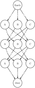
(a) Unweighted

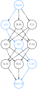
(b) Weighted

Figure 1: Relaxed decision diagrams for an ARP with asteroids $\{A,B,C\}$.

2.4 Refining a Relaxed Diagram

Simply having a relaxed DD is not enough to solve an optimization problem. Usually, if the shortest path through the relaxed diagram is feasible, then it is also optimal. However, for the ARP, the length of the shortest path might be super-optimal even if the path is feasible, as the costs on the arcs are not exact.

To get an optimal solution to the ARP, we are going to leverage three DD refinement techniques. We will illustrate them using the example from before. Let $\mathcal{M}$ be our relaxed DD, let $\pi^{*}$ be the shortest path through $\mathcal{M}$, let $\underline{z}$ be the length of $\pi^{*}$ (and thus a relaxed bound on the optimal cost). In Figure 1(b), we have a relaxed DD with a shortest path of $\pi^{*}=(A\rightarrow B\rightarrow C)$ and a cost of $\underline{z}=10$. Assume that we solve the inner problem for $\pi^{*}$ and find that $f(\pi^{*})=12$; now we know that our diagram is overestimating the quality of $\pi^{*}$, and we also have a real solution $\overline{z}$ with cost $\overline{z}=12$. In the remainder of this section, we discuss the refinement techniques, and then demonstrate how they work using our example in Figures 2(b), 2(c), and 2(d).

The first refinement technique we leverage is constraint propagation. Each node $u$ in Figure 1(b) is labeled with the length of the shortest path to that node $z_{\downarrow}(u)$. If each node is similarly labeled with the length of the shortest path from $u$ to the terminal $z_{\uparrow}(u)$, then any node where $z_{\downarrow}(u)+z_{\uparrow}(u)\geq\overline{z}$ can be removed from the diagram. This is true because there is no path passing through such a node with a cost less than our best known solution $\overline{z}$. There are other propagation techniques for solving sequencing problems with DDs that are also useful for this problem [1].

(a) Initial Diagram

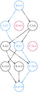
(b) Constraint Propagation

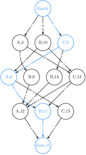
(c) Split

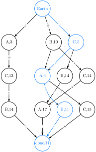
(d) Peel

Figure 2: Refining relaxed decision diagrams.

The second refinement technique we leverage is node splitting. In our example, we no longer need to include $\pi^{*}$ in our diagram because we know its true value. We remove $\pi^{*}$ from $\mathcal{M}$ to find a tighter relaxed bound on our problem. A node $u$ is split by making a copy $u^{\prime}$. The in-arcs are heuristically sorted into two sets and distributed between the two nodes. The out-arcs are copied such that both nodes have a copy of each arc. Then arcs are removed if they can be shown not to contain the optimal solution. In our example (Figure 2(c)), there is a node with two paths to reach it $\{(A\rightarrow B),(C\rightarrow B)\}$ and two out-arcs to $A$ and $C$. We split the node and give one in-arc to each, as well as a copy of both out-arcs. Then we observe that one node represents only paths starting with $(A\rightarrow B)$ and we want to remove the path $\pi^{*}=(A\rightarrow B\rightarrow C)$, so we can remove the $C$ out-arc for that node. Finally, we observe that the other node represents only paths starting with $(C\rightarrow B)$, and the path $C\rightarrow B\rightarrow C$ is infeasible, so we can remove the $C$ arc from this node as well.

The third refinement technique we leverage is the peel operation [8, 9]. In the peel operation, we start by picking a node $u$, and then iteratively split nodes from the top down until we have separated all of the paths passing through $u$ in $\mathcal{M}$ into a discrete graph that only connects at the root and terminal. The process of repeatedly peeling and splitting nodes in a relaxed DD until you reach an optimal solution is called peel-and-bound. In our example (Figure 2(d)), we peel the graph into a DD containing only paths that start with $A$, and a separate DD that contains no paths starting with $A$. Note that because we remove $\pi^{*}$, the only remaining path starting with $A$ is $(A\rightarrow C\rightarrow B)$. Also note that the process of solving a DD using peel-and-bound is extremely parallelizable. Each peeled DD can be considered a discrete problem to be solved, and so the problem can be easily divided among any number of available processors without the need for the processors to communicate (with the exception of requesting new tasks).

3 The Initial Decision Diagram

The examples in Section 2 assumed the availability of bounds on the arc costs. We also mentioned that calculating arc bounds is expensive because it uses SLSQP, and the algorithm we propose is designed to minimize the use of SLSQP. Consider that constraint propagation only ever removes arcs, it never adds them. A key insight is that when a DD is refined using splits and peels, the number of arcs in the DD may grow, but the new arcs are always copies of old arcs. Whether splitting or peeling, a valid bound on the cost of an arc is also a valid bound on its copy. So while it may be necessary or desirable to recalculate the bound on an arc at some point in the process to get a tighter bound, peels and splits can be carried out as much as memory limitations allow without the need to perform any SLSQP. We propose doing the bulk of the SLSQP upfront, thus constructing a strong initial relaxed DD, and allowing peel-and-bound to be used effectively.

We begin by constructing a relaxed DD $\mathcal{M}$ exactly as shown in Figure 1(a). We start with a root node at layer $0$, a terminal node at layer $n+1$, and $n$ nodes on each layer with index $i$, where $1\leq i\leq n$. Each node $u$ in a layer $i$ is given a label $\ell$ (where labels map to asteroids) unique to that layer. Then each node $v$ in layer $i-1$ is the origin for an arc ending at $u$, as long as $v$ has a different label. An arc with a null label is added from each node in layer $n$ to the terminal.

Now we weight the DD. The arcs going from layer $0$ to layer $1$ are straightforward. A valid bound on the cost of such an arc (the weight) $a_{uv}$ going from node $u$ to $v$ with label $l(v)$ is given by $\mathcal{Q}(Earth,l(v),0,\tau_{\Omega},0,t_{\Omega})$. The weight of each arc going from layer $n$ to $n+1$ is 0. Remember that we have $Q^{\prime}$ to retrieve the optimal transfer time when waiting is free. The latest possible start time for arcs going from layer $i-1$ to $i$ is $(i-1)(\tau_{\Omega}+t_{\Omega})$. So $\mathcal{Q}^{\prime}(l(u),l(v),0,(n-1)(\tau_{\Omega}+t_{\Omega}),0,t_{\Omega})=(\tau^{*},t^{*},z^{*})$ finds a valid weight for each arc $a_{uv}$ where $v$ is in layer $n$. Notice that the resulting $z^{*}$ is actually a valid weight for every arc going from a node with label $l(u)$ to a node with label $l(v)$ ($a_{l(u),l(v)}$). However, it is worth calculating better bounds. Consider that $Q^{\prime}$ will return the same $z^{*}$ for any arc $a_{l(u),l(v)}$ ending at layer $i$, provided that $\tau^{*}+t^{*}\leq(i-1)(\tau_{\Omega}+t_{\Omega})$. So $z^{*}$ can be used as the weight for any arc meeting that criterion, and then $Q^{\prime}$ can be queried for the next highest layer where the arc $a_{l(u),l(v)}$ is unweighted. This can be repeated until every arc is weighted.

The above construction is valid, but it is possible and worthwhile to do better. All work put into the initial diagram can be reused during peel-and-bound. Assume we find a heuristic solution $\overline{z}$. There are many methods available in the literature for doing this [10, 4]. Each node $u$ can be easily labeled as shown in Figure 2(b) with $z_{\downarrow}(u)$ and $z_{\uparrow}(u)$. Then the nodes $u$ on layer $1$ can be given an earliest start time label ($est$) by performing a binary search to find the value of $\Theta$ where $\tilde{\mathcal{Q}}(Earth,l(u),0,\Theta)=\overline{z}-z_{\uparrow}(u)$. The earliest arrival time ($eat$) to reach the end of an arc $a_{uv}$ can be similarly found by performing a binary search to find the value of $\Theta$ where $\tilde{\mathcal{Q}}(l(u),l(v),est(u),\Theta)=\overline{z}-z_{\downarrow}(u)-z_{\uparrow}(v)$. The $est$ of a node $u$ is the minimum $eat$ of arcs ending at $u$.

The weight of arcs leaving a node with a newly calculated $est$ can be recalculated using the same method as before with $\mathcal{Q}^{\prime}$, but replacing $\tau_{s}=0$ with $\tau_{s}=est$. Then all of the weights and $est$ labels can be iteratively updated until the bounds on the arc costs stop improving by a worthwhile metric. The decision of when to stop the process of constructing the initial DD is heuristic.

4 Using Peel-and-Bound

In almost all ways, the details of using peel-and-bound are heuristic decisions. No matter what choice you make, peel-and-bound will reach an optimal solution, because at each iteration, infeasible or sub-optimal solutions are removed from the diagram, and eventually the remaining shortest path length is optimal. However, decisions about when and where to peel and split have a large impact on the solve time. We propose using the same settings as used in the initial proposal outlining peel-and-bound [9]. For the search procedure, we propose using an embedded restricted decision diagram search [9]. This can be thought of as a beam-search or generalized greedy search where the search space is restricted to paths encoded in the relaxed DD. Instead of using SLSQP to evaluate the solutions as they are generated, the weights in the decision diagram are used to build a candidate list, and then the best candidate solutions are evaluated using SLSQP to search for improved solutions ($\overline{z}$).

5 Looking Forward

This paper details the first method of finding an exact solution to the Asteroid Routing Problem; all existing methods are heuristic. We are currently working on implementing our method of solving the ARP, and we believe the methods in this paper can be extended to the Dyson Ring challenge without much difficulty. These methods will also be useful to researchers interested in implementing new heuristic search techniques for global trajectory optimization.

References

- [1] Cire, A.A., van Hoeve, W.J.: Multivalued decision diagrams for sequencing problems. Operations Research 61(6), 1259, 1462 (2013)
- [2] Gillard, X.: Discrete Optimization with Decision Diagrams: Design of a Generic Solver, Improved Bounding Techniques, and Discovery of Good Feasible Solutions with Large Neighborhood Search. Phd dissertation, Université catholique de Louvain (2022)
- [3] GTOC: The global trajectory optimization competition portal (2006), https://sophia.estec.esa.int/gtoc_portal
- [4] Hennes, D., Izzo, D., Landau, D.: Fast approximators for optimal low-thrust hops between main belt asteroids. In: 2016 IEEE Symposium Series on Computational Intelligence (SSCI). pp. 1–7. IEEE (2016)
- [5] Izzo, D., López-Ibáñez, M.: Optimization challenges at the European Space Agency pp. 1542–1553 (2022)
- [6] Izzo, D.: Revisiting lambert’s problem. Celestial Mechanics and Dynamical Astronomy 121, 1–15 (2015)
- [7] López-Ibáñez, M., Chicano, F., Gil-Merino, R.: The asteroid routing problem: A benchmark for expensive black-box permutation optimization. In: International Conference on the Applications of Evolutionary Computation (Part of EvoStar). pp. 124–140. Springer (2022)
- [8] Rudich, I., Cappart, Q., Rousseau, L.M.: Peel-and-bound: Generating stronger relaxed bounds with multivalued decision diagrams. In: International Conference on Principles and Practice of Constraint Programming (2022)
- [9] Rudich, I., Cappart, Q., Rousseau, L.M.: Improved peel-and-bound: Methods for generating dual bounds with multivalued decision diagrams. Journal of Artificial Intelligence Research 77, 1489–1538 (aug 2023). https://doi.org/10.1613/jair.1.14607
- [10] Simões, L.F., Izzo, D., Haasdijk, E., Eiben, A.: Multi-rendezvous spacecraft trajectory optimization with beam p-aco. In: Evolutionary Computation in Combinatorial Optimization: 17th European Conference, EvoCOP 2017, Amsterdam, The Netherlands, April 19-21, 2017, Proceedings 17. pp. 141–156. Springer (2017)
- [11] Virtanen, P., Gommers, R., Oliphant, T.E., Haberland, M., Reddy, T., Cournapeau, D., Burovski, E., Peterson, P., Weckesser, W., Bright, J., et al.: Scipy 1.0: fundamental algorithms for scientific computing in python. Nature methods 17(3), 261–272 (2020)