Structural transitions in interacting lattice systems

Abstract

We consider two-dimensional systems of point particles located on rectangular lattices and interacting via pairwise potentials. The goal of this paper is to investigate the phase transitions (and their nature) at fixed density for the minimal energy of such systems. The 2D rectangle lattices we consider have an elementary cell of sides $a$ and $b$, the aspect ratio is defined as $\Delta=b/a$ and the inverse particle density $A=ab$; therefore, the “symmetric” state with $\Delta=1$ corresponds to the square lattice and the “non-symmetric” state to the rectangular lattice with $\Delta\neq 1$. For certain types of the interaction potential, by changing continuously the particle density, such lattice systems undertake at a specific value of the (inverse) particle density $A^{*}$ a structural transition from the symmetric to the non-symmetric state. The structural transition can be either of first order ($\Delta$ unstick from its symmetric value $\Delta=1$ discontinuously) or of second order ($\Delta$ unstick from $\Delta=1$ continuously); the first and second-order phase transitions are separated by the so-called tricritical point. We develop a general theory on how to determine the exact values of the transition densities and the location of the tricritical point. The general theory is applied to the double Yukawa and Yukawa-Coulomb potentials.

74G65, 74N05, 82B26

1 Introduction

Lattice systems of interacting particles are known as good models to understand physical [4, 9, 22, 23, 28] or biological [7, 26] phenomena in the simplest periodic setting (see also [13] and references therein). In particular, the ground state approach – where a lattice energy has to be minimized in order to find the most stable state of the system – is of high interest in applied mathematics.

Considering a radially symmetric interaction potential $f$ with parameters, a set of lattices $\mathcal{L}\subset\mathbb{R}^{d}$, and defining the energy of this lattice system as

$$\forall L\in\mathcal{L},\quad E[L]=\frac{1}{2}\sum_{p\in L\backslash\{0\}}f(|p|),$$

where $|\cdot|$ is the Euclidean norm on $\mathbb{R}^{2}$, one can ask the following important questions:

• what is the minimizer of $E$ in the class $\mathcal{L}$?

• does this minimizer changes when parameters of $f$ vary?

• does the minimizer changes when the lattice’s density varies?

These questions have recently received a certain interest in the mathematical community [4, 6, 9, 24, 25] as well as their more general associated problem known as crystallization (see [8] and references therein), best packings [15, 33] and universal optimality [14, 16]. The questions of phase transitions, i.e. studying the energy minimizers as density or parameters vary, have been shown as both interesting [5, 31] and difficult [11, 24] to solve.

Very few results exist in that direction. The Lennard-Jones system – i.e. for a difference of inverse power laws – is now entirely understood in dimension 2 [12, 24] in terms of minimizers at fixed density whereas many problems in the field are still open, with a lack of general theory. Furthermore, only few – but very important – results are known in higher dimensions, especially in dimensions 8 and 24 where best packing and universal optimality are proven [10, 16]. The rest of our knowledge is restricted to numerical investigations (see e.g. [11]).

The goal of this paper is to derive technical, theoretical and numerical results for phase transition problems in lattice systems. More precisely, we are tackling here both first and second order phase transitions for smooth potentials $f$ among two-dimensional rectangular lattices, splitting ground states into square and non-square structures. Following Landau’s free energy approach in statistical physics [1, 20, 21, 30], we expand our energy $E$ in terms of a (small) lattice parameter and we study the corresponding transition points (second-order phase transition), i.e. the value of the inverse density where transition occurs. Furthermore, we focus on important transition points called tricritical points where (continuous) second-order transition becomes of (discontinuous) first-order.

Our findings are both theoretical and numerical. After defining the classes of interaction potentials and lattices we are studying in this work, we obtain the following results:

1. Theoretically, we show how a Taylor expansion of the energy $E$ can be performed in terms of the lattice parameter $\varepsilon$ ($\varepsilon=0$ corresponding to the square lattice). Results are derived ensuring the existence of transition/tricritical points and showing the universal behavior of the energy minimizer in the neighborhood of these points.
   

2. Numerically, we are investigating both double Yukawa and Yukawa-Coulomb potentials. Since they are highly inhomogeneous, a numerical study is performed in order to plot phase diagrams, second-order phase transition curves and tricritical points.

In both cases, asymptotics results in the neighborhood of transition/tricritical points as well as singular values of potential’s parameters are derived.

The method can be generalized easily to other types of lattices, like the 2D (equilateral) triangle lattice which is the centered rectangle lattice with the aspect ratio $\sqrt{3}$ against the general centered rectangle lattice. The generalization of the method to 3D lattice structure is also straightforward. The application of the theory to other types of interaction potentials, especially to Lennard-Jones potential, is of our future interest.

Plan of the paper. In Section 2, we give the precise definitions of potentials, lattices and energies we are considering. General results on phase transitions are proved in Section 3 whereas applications to double Yukawa and Yukawa-Coulomb potentials are presented in Sections 4 and 5, respectively, with both numerical and theoretical aspects.

2 Preliminary formalism

In this section, we briefly present the type of potential, lattices and energy we are considering in this paper.

Let us start with potentials. Our goal is to cover the main interaction potentials presented for instance in [19] (see also [4]).

Definition 2.1 (Admissible potential).

We say that $f\in\mathcal{F}$ if $f:(0,\infty)\to\mathbb{R}$, $|f(r^{2})|=O(r^{-2-\varepsilon})$ for some $\varepsilon>0$ as $r\to\infty$, and there exists a Radon measure $\mu_{f}$ on $(0,+\infty)$ such that

$$f(r)=\int_{0}^{\infty}e^{-r^{2}t}\ {\rm d}\mu_{f}(t).$$ (2.1)

Furthermore, we say that $f\in\mathcal{F}_{+}$ if $\mu_{f}$ is non-negative.

Remarks 2.2 (Completely monotone potentials).

Let us write $f(r)=F(r^{2})$ where $F:(0,+\infty)\to\mathbb{R}$, then:

1. the measure $\mu_{f}$ is actually the inverse Laplace transform of $F$;

2. By Bernstein-Hausdorff-Widder theorem [2], we know that $f\in\mathcal{F}_{+}$ if and only if $F$ is completely monotone, i.e. the derivatives of $F$ alternate their sign: $\forall k\in\mathbb{N}$, $\forall r>0$, $(-1)^{k}F^{(k)}(r)\geq 0$.

Examples 2.3 (Riesz and Yukawa potentials).

Let us mention two important interaction potential we will consider in this work:

1. the Riesz potential with parameter $s>0$ is given by

   $$f(r)=\frac{1}{r^{s}},\qquad d\mu_{f}(t)=\frac{1}{\Gamma(s/2)}t^{s/2-1}dt$$ (2.2)

   with $\Gamma$ being the Euler Gamma function. We notice that $f\in\mathcal{F}_{+}$ if and only if $s>2$. Nevertheless, we will also consider lower exponents by renormalizing our lattice energy (see Remark 2.10) even though $f\not\in\mathcal{F}$ in that case, because of its non-integrability at infinity.

2. the Yukawa potential, belonging to $\mathcal{F}_{+}$ reads, for $\kappa>0$, as

   $$f(r)=\frac{e^{-\kappa r}}{r},\qquad d\mu_{f}(t)=\frac{1}{\sqrt{\pi t}}\exp\left(-\frac{\kappa^{2}}{4t}\right)dt.$$ (2.3)

The set of lattice structures we are considering is defined as follows.

Definition 2.4 (Family of rectangular lattices).

Let $\Delta\in(0,1]$ and $A>0$. The rectangular lattice of area $A$ and side-lengths $\sqrt{A\Delta}$ and $\sqrt{\frac{A}{\Delta}}$ is defined as

$$L_{\Delta,A}:=\sqrt{A}\left[\mathbb{Z}\left(\frac{1}{\sqrt{\Delta}},0\right)\oplus\mathbb{Z}\left(0,\sqrt{\Delta}\right)\right],$$

and its associated quadratic form is defined by

$$\forall(j,k)\in\mathbb{Z}^{2},\quad Q_{\Delta,A}(j,k):=\left|j\sqrt{A}\left(\frac{1}{\sqrt{\Delta}},0\right)+k\sqrt{A}\left(0,\sqrt{\Delta}\right)\right|^{2}=A\left(\frac{j^{2}}{\Delta}+k^{2}\Delta\right),$$

where $|\cdot|$ is the euclidean norm on $\mathbb{R}^{2}$.

Remark 2.5.

Notice that this family of lattices is exactly, up to isometry, the set of all rectangular lattices with fixed density. Furthermore, the particle system is invariant under rotation by the right angle $\pi/2$ which is equivalent to the interchange $\Delta$ and $1/\Delta$. The special case $\Delta=1$ corresponds to the “symmetric” state of the square lattice, the case $\Delta\neq 1$ corresponds to the “non-symmetric” state of the rectangle lattice.

The lattice energy we are studying in this paper is the energy per point of $L_{A,\Delta}$ interacting via potential $f$.

Definition 2.6 (Interaction energy).

Let $f\in\mathcal{F}$, $A>0$, $\Delta\in(0,1]$, then the $f$-energy of $L_{A,\Delta}$ is defined by

$$E(A,\Delta):=\frac{1}{2}\mathop{\sum\nolimits^{\prime}}_{j,k=-\infty}^{\infty}f\left(\sqrt{Q_{A,\Delta}(j,k)}\right)=\frac{1}{2}\mathop{\sum\nolimits^{\prime}}_{j,k=-\infty}^{\infty}f\left(\sqrt{A\left(\frac{j^{2}}{\Delta}+k^{2}\Delta\right)}\right).$$ (2.4)

Remark 2.7.

The prefactor $1/2$ appears because each energy term is shared by two particles and the prime at the sum means that the self-energy term $j=k=0$ is omitted. Note that the dependence of the energy on the parameters of the potential $f$ is not written explicitly, for simplicity reasons.

As already done in other papers [4, 17] for rectangular or general lattices, this energy can be written in terms of Jacobi theta functions thanks to the Laplace transform expression of $f$.

Lemma 2.8 (Integral representation of the energy, see e.g. [4, 17]).

Let $f\in\mathcal{F}$, $A>0$, $\Delta\in(0,1]$, then we have

$$E(A,\Delta)=\frac{1}{2}\int_{0}^{\infty}\left[\theta_{3}\left({\rm e}^{-t/\Delta}\right)\theta_{3}\left({\rm e}^{-t\Delta}\right)-1\right]{\rm d}\mu_{f}\left(\frac{t}{A}\right),$$ (2.5)

where

$$\theta_{3}(q)=\sum_{j=-\infty}^{\infty}q^{j^{2}}$$ (2.6)

denotes Jacobi elliptic function with zero argument.

Remark 2.9.

We use Gradshteyn-Ryzhik [18] notation for the third Jacobi theta function. Furthermore the subtraction of $-1$ in the square bracket is due to the absence of the self-energy term $(j,k)=(0,0)$ in the sum (2.4). If $\mu_{f}$ is absolutely continuous with respect to the Lebesgue measure, i.e. $d\mu_{f}(t)=\rho_{f}(t)dt$, then we have

$${\rm d}\mu_{f}\left(\frac{t}{A}\right)=\rho_{f}\left(\frac{t}{A}\right)\frac{{\rm d}t}{A}.$$ (2.7)

Moreover, note that the invariance of $E(A,\Delta)$ with respect to the transform $\Delta\to 1/\Delta$ is obviously ensured by the formula (2.5).

Remark 2.10.

If the potential $f$ decays to zero at large distances too slowly, the integral in (2.5) may diverge which requires a regularization (analytic continuation). Like for instance, for the Riesz potential the integral converges if $s>2$. The Coulomb case with $s=1$ has to be regularized by adding a uniform neutralizing background which corresponds to the subtraction of the singular term $-\pi/t$ in the square bracket in the integral (2.5), as it is explained for instance in [32].

3 General theory of structural transitions

To account better for the symmetry $\Delta\to 1/\Delta$ of the energy (2.5), we introduce the parameter $\varepsilon$ via

$$\Delta=e^{\varepsilon}.$$ (3.1)

Thus the $\Delta\to 1/\Delta$ symmetry of the energy (2.5) is converted to the $\varepsilon\to-\varepsilon$ one of the energy

$$E(A,e^{\varepsilon})=\frac{1}{2}\int_{0}^{\infty}\left[\theta_{3}\left({\rm e}^{-t\exp(-\varepsilon)}\right)\theta_{3}\left({\rm e}^{-t\exp(\varepsilon)}\right)-1\right]{\rm d}\mu_{f}\left(\frac{t}{A}\right).$$ (3.2)

At the same time, the symmetric (square lattice) value of the parameter $\Delta=1$ is consistent with $\varepsilon=0$.

Let us recall the universal optimality result (among lattices) concerning the square lattice, due to Montgomery [27].

Proposition 3.1 (Universal optimality among rectangular lattices).

If $f\in\mathcal{F}_{+}$, then $\varepsilon=0$ is the unique minimizer of $\varepsilon\mapsto E(A,e^{\varepsilon})$ for all $A>0$.

Proof.

Since $\mu_{f}$ is nonnegative and $\Delta=1$ is the unique minimizer of the positive function $\Delta\mapsto\theta_{3}(e^{-t\Delta})\theta_{3}(e^{-t\Delta^{-1}})-1$ as shown in [27], it follows that for all $\Delta>0$, $E(A,\Delta)\geq E(A,1)$ with equality if and only if $\Delta=1$. Applying the change of variable $\Delta=\exp(\varepsilon)$ completes the proof. ∎

The following result gives the expansion of $E(A,e^{\varepsilon})$, for fixed $A$ and as $\varepsilon\to 0$.

Theorem 3.2 (Taylor expansion of the energy).

Let $f\in\mathcal{F}$ and $A>0$, then, as $\varepsilon\to 0$,

$$E(A,e^{\varepsilon})=E_{0}(A)+E_{2}(A)\varepsilon^{2}+E_{4}(A)\varepsilon^{4}+O(\varepsilon^{6}),$$ (3.3)

where

$$E_{0}(A)=E(A,1)=\frac{1}{2}\int_{0}^{\infty}\left[\left(\theta_{3}\right)^{2}-1\right]{\rm d}\mu_{f}\left(\frac{t}{A}\right)$$ (3.4)

is the energy of the square lattice,

$$E_{2}(A)=\frac{d^{2}}{d\varepsilon^{2}}\left[E(A,e^{\varepsilon})\right]_{|\varepsilon=0}=\frac{1}{2}\int_{0}^{\infty}\left[t\theta_{3}\theta_{3}^{(1)}-t^{2}\left(\theta_{3}^{(1)}\right)^{2}+t^{2}\theta_{3}\theta_{3}^{(2)}\right]{\rm d}\mu_{f}\left(\frac{t}{A}\right),$$ (3.5)

and

$$E_{4}(A)=\frac{d^{4}}{d\varepsilon^{4}}\left[E(A,e^{\varepsilon})\right]_{|\varepsilon=0} = \frac{1}{24}\int_{0}^{\infty}\left[t\theta_{3}\theta_{3}^{(1)}-t^{2}\left(\theta_{3}^{(1)}\right)^{2}+7t^{2}\theta_{3}\theta_{3}^{(2)}+6t^{3}\theta_{3}\theta_{3}^{(3)}-6t^{3}\theta_{3}^{(1)}\theta_{3}^{(2)}\right.$$ (3.6)

$$\left.+t^{4}\theta_{3}\theta_{3}^{(4)}-4t^{4}\theta_{3}^{(1)}\theta_{3}^{(3)}+3t^{4}\left(\theta_{3}^{(2)}\right)^{2}\right]{\rm d}\mu_{f}\left(\frac{t}{A}\right),$$

and where the theta function and its derivatives are written for simplicity as

$$\theta_{3}:=\theta_{3}\left({\rm e}^{-t}\right),\qquad\theta_{3}^{(n)}:=\frac{{\rm d}^{n}}{{\rm d}t^{n}}\theta_{3}\left({\rm e}^{-t}\right),n\in\mathbb{N}.$$ (3.7)

Remark 3.3.

Note that because of the $\varepsilon\to-\varepsilon$ symmetry of the energy, the expansion contains only even powers of $\varepsilon$.

Proof.

We use the fact that $f$ is analytic and $f(\cdot^{2})$ is absolutely summable at infinity. Therefore, the wished expansion easily yields from the one of the theta functions product, i.e. for all $t>0$ and as $\varepsilon\to 0$, the quantity $\theta_{3}\left({\rm e}^{-t\exp(-\varepsilon)}\right)\theta_{3}\left({\rm e}^{-t\exp(\varepsilon)}\right)$ is given by

$$\sum_{j,k}{\rm e}^{-j^{2}t\exp(-\varepsilon)}{\rm e}^{-k^{2}t\exp(\varepsilon)} = \sum_{j,k}{\rm e}^{-(j^{2}+k^{2})t}\Big{[}1+\left(j^{2}-k^{2}\right)t\varepsilon$$ (3.8)

$$+\frac{1}{2}\left(-j^{2}-k^{2}-2j^{2}k^{2}t+j^{4}t+k^{4}t\right)t\varepsilon^{2}$$

$$+\frac{1}{6}\left(j^{2}-k^{2}\right)\left(1-3j^{2}t-3k^{2}t-2j^{2}k^{2}t^{2}+j^{4}t^{2}+k^{2}t^{2}\right)t\varepsilon^{3}$$

$$+\frac{1}{24}\left(-j^{2}-k^{2}-2j^{2}k^{2}t+7j^{4}t+7k^{4}t-6j^{6}t^{2}-6k^{6}t^{2}\right.$$

$$\left.+6j^{4}k^{2}t^{2}+6j^{2}k^{4}t^{2}+j^{8}t^{3}+k^{8}t^{3}-4j^{6}k^{2}t^{3}\right.$$

$$\left.-4j^{2}k^{6}t^{3}+6j^{4}k^{4}t^{3}\right)t\varepsilon^{4}+O\left(\varepsilon^{6}\right)\Big{]}.$$

The terms of odd orders $\varepsilon$ and $\varepsilon^{3}$ vanish because of the antisymmetry of summands with respect to the interchange of indices $j$ and $k$. The terms of even orders $\varepsilon^{2}$ and $\varepsilon^{4}$ can be further simplified by using the interchange of indices $j$ and $k$ and the sums of type $\sum_{j}j^{2n}\exp(-j^{2}t)$ with $n\in\mathbb{N}^{*}$ are equal to $(-1)^{n}\theta_{3}^{(n)}$. ∎

Remark 3.4 (Connection with Statistical Physics).

The present exact expansion (3.3) has its counterpart in statistical physics where it represents a mean-field approximation for a complicated statistical model in thermal equilibrium at some temperature, known as the Landau free energy [1, 20]. The parameter $\varepsilon$ plays there the role of the order parameter which vanishes in the disordered phase and takes non-zero values in the ordered phase. The general analysis of the expansion (3.3) in the context of critical phenomena in statistical models can be found in many textbooks, see e.g. [21, 30]. In what follows, we shall adopt this general analysis to our ground-state problem.

By (3.3), we have that, for all $A>0$, as $\varepsilon\to 0$,

$$E(A,e^{\varepsilon})-E(A,1)=E_{2}(A)\varepsilon^{2}+E_{4}(A)\varepsilon^{4}+O(\varepsilon^{6})=\varepsilon^{2}\left[E_{2}(A)+E_{4}(A)\varepsilon^{2}+O(\varepsilon^{4})\right].$$

Therefore, it appears that the sign of $E_{2}(A)$ determines the one of $E(A,e^{\varepsilon})-E(A,1)$ for sufficiently small values of $\varepsilon>0$, giving the optimality of the square lattice when $E(A,e^{\varepsilon})-E(A,1)>0$ and the optimality of a non-square one when $E(A,e^{\varepsilon})-E(A,1)<0$.

Definition 3.5.

Let $f\in\mathcal{F}\backslash\mathcal{F}_{+}$, then any $A^{*}$ such that

$$E_{2}(A^{*})=0$$ (3.9)

with a change of sign for $E_{2}$ at $A=A^{*}$ is called a transition point.

A simple condition can be written for insuring the existence of such transition point.

Proposition 3.6 (Existence of a transition point).

Let $f\in\mathcal{F}$. Then:

1. if $f\in\mathcal{F}_{+}$, then there is no transition point;

2. if $f\in\mathcal{F}\backslash\mathcal{F}_{+}$ such that $\mu_{f}<0$ on $(0,r_{0})$ or on $(r_{1},+\infty)$ for some $r_{0},r_{1}>0$, then a transition point exists.

Proof.

It has been shown by Faulhuber and Steinerberger [17] that

$$\forall t>0,\quad t\theta_{3}\theta_{3}^{(1)}+t^{2}\theta_{3}\theta_{3}^{(2)}-t^{2}\left(\theta_{3}^{(1)}\right)^{2}>0.$$

Therefore, if $f\in\mathcal{F}_{+}$, then $\mu_{f}$ is nonnegative and it follows that $E_{2}(A)>0$ for all $A>0$.
Furthermore, the second point follows from [6, Prop. 4.4] applied to the square lattice among rectangular lattices in dimension $d=2$. ∎

Examples 3.7.

Point $(1)$ of the previous result can be illustrated by any Riesz potential, whereas point $(2)$ is covered for instance by the double-Yukawa potential we study in the next section of the paper, given for all $r>0$ by

$$f(r)=v_{1}\frac{\exp{(-\kappa_{1}r)}}{r}-v_{2}\frac{\exp{(-\kappa_{2}r)}}{r},\quad v_{1}>v_{2}>0,\qquad\kappa_{1}>\kappa_{2}>0.$$

We now give conditions such that a second order phase transition (see [29]), i.e. the transition for the minimizer of $\varepsilon\to E(A,e^{\varepsilon})$ is continuous.

Proposition 3.8 (Second order phase transition).

Let $f\in\mathcal{F}$ and $A^{*}$ be a transition point such that:

1. $E_{2}$ is strictly decreasing in the neighborhood of $A^{*}$;

2. $E_{4}(A^{*})>0$.

Then there exists $A_{0}>0$ and $A_{1}>0$ such that

• if $A_{0}<A<A^{*}$, then $\varepsilon=0$ is the unique minimizer of $\varepsilon\to E(A,e^{\varepsilon})$;

• if $A^{*}<A<A_{1}$, a minimizer $\varepsilon$ of $\varepsilon\to E(A,e^{\varepsilon})$ satisfies the following asymptotics, as $A\to A^{*}$:

  $$\varepsilon=\sqrt{\frac{-\frac{dE_{2}}{dA}(A^{*})}{2E_{4}(A^{*})}}\sqrt{A-A^{*}}+o(\sqrt{A-A^{*}}).$$

Remark 3.9.

The same result can be written when $E_{2}$ is strictly increasing in the neighborhood of $A^{*}$, with the reverse condition $E_{4}(A^{*})<0$, which simply exchanges the regimes of optimality.

Proof.

Since a transition point exists, a simple Taylor expansion of $E_{2}$ as $A\to A^{*}$ reads

$$E_{2}(A) =E_{2}(A^{*})+\frac{dE_{2}}{dA}(A^{*})(A-A^{*})+o(A-A^{*})$$

$$=-\frac{dE_{2}}{dA}(A^{*})(A^{*}-A)+o(A-A^{*}).$$

By assumption, we know that $\frac{dE_{2}}{dA}(A^{*})<0$ and let us write $b:=-\frac{dE_{2}}{dA}(A^{*})>0$ for simplicity in such a way that, as $A\to A^{*}$,

$$E_{2}(A)=b(A^{*}-A)+o(A^{*}-A).$$ (3.10)

The value of $\varepsilon$ which minimizes $E(A,\cdot)$ satisfies the following asymptotic stationarity condition we get from (3.3):

$$\frac{\partial E(A,e^{\varepsilon})}{\partial\varepsilon}=2E_{2}(A)\varepsilon+4E_{4}(A)\varepsilon^{3}+O(\varepsilon^{5})=0.$$ (3.11)

Using (3.10), this condition, for $A$ in the neighborhood of $A^{*}$, is therefore equivalent to the couple of equations

$$\varepsilon=0\qquad\textnormal{or}\qquad\varepsilon^{2}=\frac{b}{2E_{4}(A^{*})}\left(A-A^{*}\right)+o(A-A^{*}).$$ (3.12)

We know that the first solution is dominant in a certain region $A_{0}<A<A^{*}$ with $A_{0}\geq 0$. Since $\varepsilon^{2}$ must be a real positive number and $E_{4}(A^{*})>0$, the second solution is

$$\varepsilon=\sqrt{\frac{b}{2E_{4}(A^{*})}}\left(A-A^{*}\right)^{1/2}+o(\left(A-A^{*}\right)^{1/2}),$$ (3.13)

dominant in the region $A^{*}<A<A_{1}$ for a certain $A_{1}>0$, which completes the proof. ∎

Remark 3.10.

Notice that indeed the transition at $A=A^{*}$ from $\varepsilon=0$ to $\varepsilon$ given by Eq. (3.13) is continuous. Consequently, the energy and its first derivative with respect to $A$ are continuous as well.
Furthermore, the singular behaviour $\varepsilon\propto(A-A^{*})^{\beta}$ as $A\to A^{*}$, $A>A^{*}$, of the minimizer defines the critical exponent $\beta$ which in our case acquires the mean-field value $1/2$. This critical exponent is universal in the sense that it does not depend on the particular form of the interaction potential $f$ as long as the (general) assumptions are satisfied.

Let us now assume that our interaction potential $f=f_{\alpha}$ depends on a parameter $\alpha\in\mathbb{R}$. Thus, a transition point satisfying the assumptions of second-order transition is $\alpha$-dependent and one can plot the graph of $\alpha\mapsto A^{*}(\alpha)$. We therefore get a curve of second-order transitions between square and non-square rectangular lattices as minimizers of $E(A,\cdot)$. In analogy with statistical mechanics, we expect only one curve of second-order transition. This curve exists say for $\alpha>\alpha^{t}$ and necessarily terminates at some $\alpha=\alpha^{t}$ once $A^{*}(\alpha=\alpha^{t})$ satisfies, besides $E_{2}(A^{*}(\alpha^{t}))=0$, also the condition $E_{4}(A^{*}(\alpha^{t}))=0$ which changes sign at this point.

Definition 3.11.

Let $f_{\alpha}\in\mathcal{F}$ depending on a real parameter $\alpha$. We say that $A^{t}>0$ and $\alpha^{t}$ are coordinates of a tricritical point if it is a transition point satisfying both conditions

$$E_{2}(A^{t}(\alpha^{t}))=0\qquad\textnormal{and}\qquad E_{4}(A^{t}(\alpha^{t}))=0,$$ (3.14)

with a change of sign for $E_{4}$ at $A^{t}(\alpha^{t})$.

Beyond this point, i.e., for $\alpha<\alpha^{t}$, transitions between the square and rectangle lattices become of first order, i.e., there is a discontinuity in $\varepsilon$ from 0 to a finite value. This means that our expansion (3.3) no longer applies and the curve of first-order transitions can be located only numerically by plotting the energy in the whole interval $\Delta\geq 1$. Using the same method as before, we can derive the singular behavior of $\varepsilon$ at the tricritical value of $\alpha=\alpha^{t}$, in the region $A>A^{t}$.

Proposition 3.12 (Transition at the tricritical point).

Let $f_{\alpha}\in\mathcal{F}$ depending on a real parameter $\alpha$ and $(\alpha^{t},A^{t})$ be the coordinates of a tricritical point such that

1. $E_{2}$ is strictly decreasing function of $A$ in the neighborhood of $A^{t}$;

2. $E_{6}(A^{t})=\frac{d^{6}}{d\varepsilon^{6}}\left[E(A,e^{\varepsilon})\right]_{|\varepsilon=0}>0$.

Therefore, there exists $A_{2}>0$ such that for $A^{t}<A<A_{2}$, a minimizer of $\varepsilon\to E(A,e^{\varepsilon})$ satisfies the following asymptotics as $A\to A^{t}$:

$$\varepsilon=\sqrt[4]{\frac{-\frac{dE_{2}}{dA}(A^{t})}{3E_{6}(A^{t})}}(A-A^{t})^{1/4}+o\left((A-A^{t})^{1/4}\right).$$

Remark 3.13.

As Proposition 3.8, the same result for the $A<A^{t}$ regime can be written when $E_{2}$ is strictly increasing in the neighborhood of $A^{t}$ and $E_{6}(A^{t})<0$.

Proof.

This follows from (3.10) and (3.11) expanded to order $5$ – coming from the Taylor expansion of the energy to order $6$ as $E(A,e^{\varepsilon})=E_{0}(A)+E_{2}(A)\varepsilon^{2}+E_{4}(A)\varepsilon^{4}+E_{6}(A)\varepsilon^{6}+o(\varepsilon^{8})$ – and following exactly the same lines as in the proof of Proposition 3.8. ∎

Remark 3.14.

For $\alpha=\alpha^{t}$, we therefore get the singular behavior $\varepsilon\propto(A-A^{t})^{1/4}$ as $A\to A^{t}$, $A>A^{t}$, so that the critical exponent at the tricritical point is $\beta^{t}=1/4$ which is again universal up to the assumptions.

The existence of transition and tricritical points and the second-order transition curves depends on the form of the interaction potential $f$ (see e.g. Proposition 3.6 for the transition point). In the next two sections, we shall present explicit results for the double Yukawa and Yukawa-Coulomb potentials which are combinations of two (repulsive and attractive) terms. Lattice systems with these potentials exhibit in certain regions of model’s parameters continuous as well as discontinuous structural transition from the square to rectangular lattices.

4 Double Yukawa potential

Potential, parameters constraints and energy. The double Yukawa interaction potential $f\in\mathcal{F}$ is defined on $(0,+\infty)$ by

$$f(r)=v_{1}\frac{\exp{(-\kappa_{1}r)}}{r}-v_{2}\frac{\exp{(-\kappa_{2}r)}}{r},\quad v_{1}>v_{2}>0,\quad\kappa_{1}>\kappa_{2}>0,$$ (4.1)

where we choose the parameters in such a way that the first repulsive term dominates at small distances whereas the second is attractive for large one. Furthermore, the corresponding measure, given by the inverse Laplace transform of $r\mapsto f(\sqrt{r})$, reads as

$${\rm d}\mu_{f}(t)=\left[v_{1}\exp{\left(-\frac{\kappa_{1}^{2}}{4t}\right)}-v_{2}\exp{\left(-\frac{\kappa_{2}^{2}}{4t}\right)}\right]\frac{{\rm d}t}{\sqrt{\pi t}}.$$ (4.2)

The potential (4.1) is supposed to have an attractive minimum $f(r_{\min})<0$ at some $r=r_{\min}$. For simplicity, we set $r_{\min}=1$ and $f(1)=-1$, reducing in this way the number of parameters four by two. We keep the independent parameters $(v_{1},\kappa_{1})$ since

$$\kappa_{2}=\frac{\kappa_{1}v_{1}-{\rm e}^{\kappa_{1}}}{v_{1}+{\rm e}^{\kappa_{1}}}\quad\textnormal{and}\quad v_{2}=\frac{{\rm e}^{\kappa_{2}-\kappa_{1}}(1+\kappa_{1})v_{1}}{1+\kappa_{2}}.$$ (4.3)

Since $\kappa_{2}>0$, the parameters $v_{1}$ and $\kappa_{1}$ are constrained to the subspace

$$v_{1}>\frac{{\rm e}^{\kappa_{1}}}{\kappa_{1}}.$$ (4.4)

The energy per particle for the double Yukawa potential reads, given (4.3), as

$$E(A,\Delta;v_{1},\kappa_{1})=\frac{1}{2\sqrt{A\pi}}\int_{0}^{\infty}\left(v_{1}e^{-\frac{\kappa_{1}^{2}A}{4t}}-v_{2}e^{-\frac{\kappa_{2}^{2}A}{4t}}\right)\left[\theta_{3}\left({\rm e}^{-t\Delta}\right)\theta_{3}\left({\rm e}^{-t/\Delta}\right)-1\right]\frac{{\rm d}t}{\sqrt{t}}.$$ (4.5)

Notice that the exponential terms with non-zero $\kappa_{1}$ and $\kappa_{2}$ make the integral convergent for small $t$ when $\theta_{3}\left({\rm e}^{-t\Delta}\right)\theta_{3}\left({\rm e}^{-t/\Delta}\right)\sim 1/t$ as $t\to 0$.

                                           

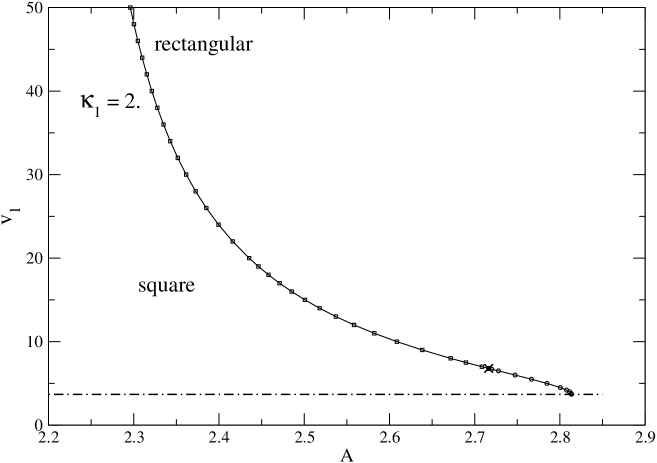
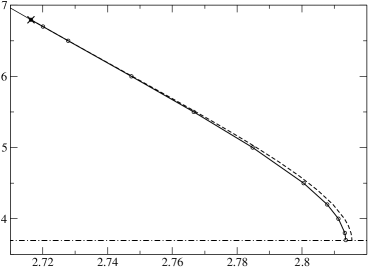
Figure 1: Phase diagram in the $(A,v_{1})$-plane for the double Yukawa potential with the fixed parameter $\kappa_{1}=2$. The critical curve of second-order transitions between the square and rectangular lattices is marked by open squares interconnected via a solid line. The cross marks the tricritical point. The discontinuous first-order transitions are indicated by open circles. The dashed line in the inset, given by $E_{2}(A)=0$, represents an artificial extension of the second-order transitions to the region dominated by first-order transitions. The dash-dotted straight line $v_{1}={\rm e}^{\kappa_{1}}/\kappa_{1}={\rm e}^{2}/2$ denotes the border of $v_{1}$-values.

Let us now show that the system always admits a transition point.

Lemma 4.1 (Existence of transition points).

For any fixed $(v_{1},\kappa_{1})$, $E$ admits a transition point $A^{*}(v_{1},\kappa_{1})$.

Proof.

For $t>0$, we have, since $v_{1}>v_{2}$ and $\kappa_{1}>\kappa_{2}$,

$$v_{1}\exp{\left(-\frac{\kappa_{1}^{2}}{4t}\right)}-v_{2}\exp{\left(-\frac{\kappa_{2}^{2}}{4t}\right)}<0\iff t<\frac{(\kappa_{1}^{2}-\kappa_{2}^{2})}{4\ln\left(\frac{v_{1}}{v_{2}}\right)}=:r_{0}.$$

It follows that $\mu_{f}<0$ on $(0,r_{0})$ and therefore, by Proposition 3.6, $E$ admits a transition point. ∎

Numerical investigation. Let us fix one of the two independent Yukawa parameters, say $\kappa_{1}=2$. By Lemma 4.1, for any given $v_{1}$, $E$ admits a transition point $A^{*}(v_{1})$. The phase diagram in the $(A,v_{1})$-plane is pictured in Fig. 1. Eq. (3.9) was used to calculate the critical curve of second-order transitions defined by

$$\mathcal{C}:=\{(A^{*},v_{1}(A^{*})):A^{*}\textnormal{ transition point}\}$$

between the square and rectangular phases, marked by open squares interconnected via a solid line. For a fixed $v_{1}$, the square (rectangular) lattice minimizes the energy in the whole interval $0\leq A\leq A^{*}$ ($A>A^{*}$). We observe the following:

1. $A^{*}\mapsto v_{1}(A^{*})$ is decreasing.

2. There exists a finite “minimal” value of $A^{*}$, $A^{*}_{\min}\approx 2.18626$, such that

   $$\lim_{A\to A^{*}_{\min}\atop A>A^{*}_{\min}}v_{1}(A_{\min}^{*})=+\infty.$$

3. The critical curve $\mathcal{C}$ ends up at the tricritical point with the coordinates $A^{t}\approx 2.7163619942262467$ and $v_{1}^{t}:=v_{1}(A^{t})\approx 6.7951845011079$, denoted by the cross.

For ${\rm e}^{\kappa_{1}}/\kappa_{1}<v_{1}<v_{1}^{t}$, the transition between the square and rectangular lattices is of the first order, see open circles in Fig. 1. For comparison, an artificial prolongation of the critical curve $v_{1}(A^{*})$ into this region is indicated by the dashed line in the inset of the figure.

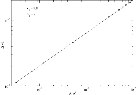
Figure 2: The double Yukawa potential with the parameters $\kappa_{1}=2$ and $v_{1}=9.8$, corresponding to the critical value of $A^{*}\approx 2.61449322978$. The log-log plot of $\Delta-1$ versus $A-A^{*}$ is presented, numerical data are represented by open circles interconnected via a dashed line. The fitting via $\Delta-1\propto(A-A^{*})^{\beta}$ yields the critical exponent $\beta^{*}\approx 0.50003$.

Singularity in the $A>A^{*}$ and $A>A^{t}$ regimes. To document the singular behaviour of $\varepsilon\sim\Delta-1$ close to the critical curve, let us choose $\kappa_{1}=2$ and $v_{1}=9.8$ and the corresponding critical value of the inverse density $A^{*}\approx 2.61449322978$. For $A$ slightly larger than $A^{*}$, the rectangle energy is minimized with respect to $\Delta$. The log-log plot of the obtained $\Delta-1$ versus $A-A^{*}$ is presented in Fig. 2. The data were fitted according to $\Delta-1\propto(A-A^{*})^{\beta}$. The obtained critical exponent $\beta\approx 0.50003$ is very close to the anticipated mean-field exponent $\beta=1/2$.

Figure 3: The double Yukawa potential with the parameter $\kappa_{1}=2$, the corresponding tricritical point has coordinates $A^{t}=2.7163619942262467\ldots$ and $v_{1}^{t}=6.7951845011079\ldots$. The log-log plot of $\Delta-1$ versus $A-A^{t}$ is presented in the rectangular region $A>A^{t}$, numerical data are denoted by open circles interconnected via a dashed line. The fitting via $\Delta-1\propto(A-A^{*})^{\beta}$ yields the tricritical exponent $\beta^{t}\approx 0.253$.

As concerns the tricritical point for the double Yukawa parameter $\kappa_{1}=2$, see the cross in Fig. 1, its coordinates $A^{t}=2.7163619942262467\ldots$ and $v_{1}^{t}=6.7951845011079\ldots$ were calculated by using the formula (3.14). The numerical calculation of the deviation $\Delta-1$ in the region of the rectangular lattice $A>A_{t}$ close to the tricritical point was made. The log-log plot of numerical data in Fig. 3 can be fitted as $\Delta-1\propto(A-A^{t})^{\beta^{t}}$, the obtained exponent $\beta^{t}\approx 0.253$ is reasonably close to the expected mean-field value $\beta^{t}=1/4$.

Figure 4: The components $(A^{t},v_{1}^{t})$ of the tricritical points as the functions of the Yukawa parameter $\kappa_{1}$. The tricritical point exists only if $\kappa_{1}\in(\kappa_{1}^{L},\kappa_{1}^{U})$ where $\kappa_{1}^{L}\approx 1.436$ and $\kappa_{1}^{U}\approx 2.03414$ are the lower and upper limits, respectively. The values of $A^{t}$ are represented by squares and the ones of $v_{1}^{t}$ by circles. The dash-and-dot line corresponds to the curve $v_{1}={\rm e}^{\kappa_{1}}/\kappa_{1}$, there are no physical solutions below it.

About the transition/tricritical points and their $\kappa_{1}$-dependence. The pair of coordinates of the tricritical point $A^{t}$ and $v_{1}^{t}$ can be calculated by using Eq. (3.14) for any value of $\kappa_{1}$, the obtained results are presented in Fig. 4. It turns out that a physically meaningful solution for the tricritical point exists only if $\kappa_{1}\in(\kappa_{1}^{L},\kappa_{1}^{U})$ where $\kappa_{1}^{L}\approx 1.436$ and $\kappa_{1}^{U}\approx 2.03414$ are the lower and upper limits, respectively. While $v_{1}^{t}$ is a decreasing function of $\kappa_{1}$, $A^{t}$ is a slowly increasing function of $\kappa_{1}$. The value of $v_{1}^{t}$ diverges when $\kappa_{1}$ approaches its lower limit $\kappa_{1}^{L}$ from above. Consequently, all transitions are of first order (discontinuous) for $0<\kappa_{1}\leq\kappa_{1}^{L}$. The upper limit $\kappa_{1}^{U}$ is given by the intersection of the $v_{1}^{t}$-curve with the dash-and-dot line $v_{1}={\rm e}^{\kappa_{1}}/\kappa_{1}$ which is the border of the accessible subspace for Yukawa parameters (4.4). All transitions are of second order (continuous) for $\kappa_{1}>\kappa_{1}^{U}$; for every $\kappa_{1}$ from this interval, the critical line goes down up to the border line $v_{1}={\rm e}^{\kappa_{1}}/\kappa_{1}$, leaving no space for a tricritical point and the corresponding first-order transitions.

Recall that for $\kappa_{1}=2$ the “minimal” critical value of $A^{*}$ at which $v_{1}(A^{*})$ goes to infinity was found numerically to be nonzero, in particular $A^{*}_{\min}\approx 2.18626$. In what follows, we aim at deriving an exact formula for $A^{*}_{\min}(\kappa_{1})$ for any value of $\kappa_{1}>0$. According to (4.3), for a fixed value of $\kappa_{1}$ and in the limit of large $v_{1}$, the Yukawa parameter $\kappa_{2}$ behaves as

$$\kappa_{2}=\kappa_{1}-\frac{1}{v_{1}}(1+\kappa_{1}){\rm e}^{\kappa_{1}}+O\left(\frac{1}{v_{1}^{2}}\right)$$ (4.6)

and the Yukawa parameter $v_{2}$ is given by

$$v_{2}=v_{1}-\kappa_{1}{\rm e}^{\kappa_{1}}+O\left(\frac{1}{v_{1}}\right).$$ (4.7)

Since

$${\rm d}\mu_{f}\left(\frac{t}{A}\right)=\rho_{f}\left(\frac{t}{A}\right)\frac{{\rm d}t}{A}=\left(v_{1}e^{-\frac{\kappa_{1}^{2}A}{4t}}-v_{2}e^{-\frac{\kappa_{2}^{2}A}{4t}}\right)\frac{{\rm d}t}{\sqrt{\pi tA}},$$ (4.8)

using the asymptotic expansions (4.6) and (4.7), the expression into brackets can be expressed as

$$v_{1}e^{-\frac{\kappa_{1}^{2}A}{4t}}-v_{2}e^{-\frac{\kappa_{2}^{2}A}{4t}}=\kappa_{1}{\rm e}^{\kappa_{1}}e^{-\frac{\kappa_{1}^{2}A}{4t}}\left[1-\frac{(1+\kappa_{1})}{2t}A\right]+O\left(\frac{1}{v_{1}}\right).$$ (4.9)

With regard to Eq. (3.5), the critical condition $E_{2}(A^{*})=0$ takes in the limit $v_{1}\to\infty$ the form

$$0=\int_{0}^{\infty}\sqrt{t}e^{-\frac{\kappa_{1}^{2}A^{*}_{\min}}{4t}}\left[1-\frac{(1+\kappa_{1})}{2t}A^{*}_{\min}\right]\left[\theta_{3}\theta_{3}^{(1)}-t\left(\theta_{3}^{(1)}+t\theta_{3}\theta_{3}^{(2)}\right)^{2}\right]{\rm d}t.$$ (4.10)

This equation determines for any $\kappa_{1}>0$ the exact value of the critical inverse density $A^{*}_{\min}(\kappa_{1})$ at which $v_{1}\to\infty$. In particular, at $\kappa_{1}=2$ the obtained $A^{*}_{\min}\approx 2.186262818188$ agrees with the previous numerical estimate $A^{*}_{\min}\approx 2.18626$. The monotonous decay of $A^{*}_{\min}$ with increasing the Yukawa parameter $\kappa_{1}>0$ is presented in Fig. 5 by the solid line connecting data (open circles). The function $A^{*}_{\min}(\kappa_{1})$ tends to unity in the limit $\kappa_{1}\to\infty$. In the opposite limit $\kappa_{1}\to 0^{+}$,

$$\lim_{\kappa_{1}\to 0^{+}}A^{*}_{\min}(\kappa_{1})=\frac{2\int_{0}^{\infty}\sqrt{t}\left[\theta_{3}\theta_{3}^{(1)}+t\theta_{3}\theta_{3}^{(2)}-t\left(\theta_{3}^{(1)}\right)^{2}\right]{\rm d}t}{\int_{0}^{\infty}\frac{1}{\sqrt{t}}\left[\theta_{3}\theta_{3}^{(1)}+t\theta_{3}\theta_{3}^{(2)}-t\left(\theta_{3}^{(1)}\right)^{2}\right]{\rm d}t}\approx 5.71344.$$ (4.11)

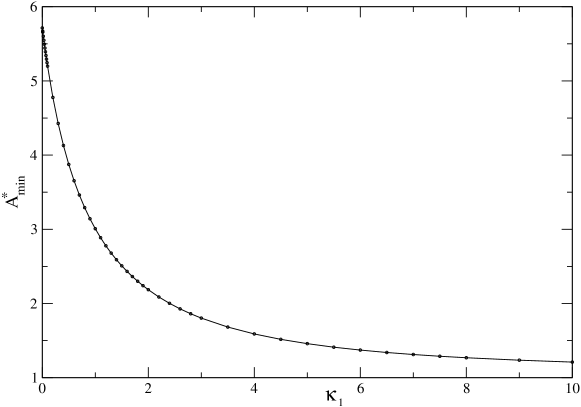
Figure 5: The dependence of the minimal value of the critical inverse density $A^{*}_{\min}$, at which a second-order transition takes place in the limit of $v_{1}\to\infty$, on the Yukawa parameter $\kappa_{1}>0$. The limiting values of $A^{*}_{\min}(\kappa_{1})$ are: $A^{*}_{\min}(\kappa_{1}\to\infty)=1$ and $A^{*}_{\min}(\kappa_{1}\to 0^{+})=5.71344\ldots$.

5 Yukawa-Coulomb potential

Potential, parameters constraints and energy. In the special Yukawa-Coulomb case $\kappa_{2}=0$, the potential

$$f(r)=v_{1}\frac{\exp{(-\kappa_{1}r)}}{r}-v_{2}\frac{1}{r}$$ (5.1)

has a minimum at $r_{\min}=1$ and $f(1)=-1$ under conditions

$$v_{1}=\frac{e^{\kappa_{1}}}{\kappa_{1}},\qquad v_{2}=\frac{1+\kappa_{1}}{\kappa_{1}}.$$ (5.2)

One is left with only one independent parameter $\kappa_{1}>0$ and there are no constraints on this parameter. The associated measure is therefore

$${\rm d}\mu_{f}(t)=\left[v_{1}\exp{\left(-\frac{\kappa_{1}^{2}}{4t}\right)}-v_{2}\right]\frac{{\rm d}t}{\sqrt{\pi t}}.$$ (5.3)

It is clear that $f\not\in\mathcal{F}$ since it is not integrable at infinity. Therefore, a regularization of the divergent lattice sum by a neutralizing background is necessary for the Coulomb term [32]. The energy then reads as

$$E(A,\Delta;\kappa_{1}) = \frac{1}{2\sqrt{A\pi}}\int_{0}^{\infty}\Bigg{\{}v_{1}{\rm e}^{-\frac{\kappa_{1}^{2}A}{4t}}\left[\theta_{3}\left({\rm e}^{-t\Delta}\right)\theta_{3}\left({\rm e}^{-t/\Delta}\right)-1\right]$$ (5.4)

$$-v_{2}\left[\theta_{3}\left({\rm e}^{-t\Delta}\right)\theta_{3}\left({\rm e}^{-t/\Delta}\right)-1-\frac{\pi}{t}\right]\Bigg{\}}\frac{{\rm d}t}{\sqrt{t}}.$$

The neutralizing background manifests itself as the addition of the singular term $-\pi/t$ in the last square bracket, which ensures the convergence of the integral. It is again straightforward to show that transitions point exists by direct application of Proposition 3.6 in the same way that we did in Lemma 4.1 for the $\kappa_{2}>0$ case.

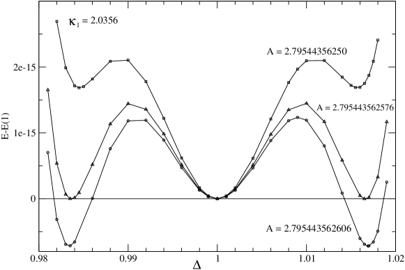
Figure 6: The plot of the energy difference $E(\Delta)-E(1)$ versus $\Delta$ for the Yukawa parameter $\kappa_{1}=2.0365$, just below its tricritical value $\kappa_{1}^{t}=2.036517758847\ldots$ where a first-order transition between the square and rectangular lattices exists. Three values of the inverse particle density $A$ are considered: $A=2.79544356250$ when the square lattice with $\Delta=1$ prevails, the first-order transition value $A_{\rm trans}=2.795443562576$ where the energies of the square and rectangular lattices, separated by energy barriers, coincide and $A=2.795443562606$ where the rectangular case is dominant via a jump in $\Delta$.

Numerical investigation. Solving the couple of equations (3.14) with $\kappa_{2}=0$, $v_{1}$ and $v_{2}$ given by (5.2), one gets the tricritical point for the Yukawa-Coulomb interaction: $A^{t}\approx 2.795433950879$ and $\kappa_{1}^{t}\approx 2.036517758847$. Let us make a small step into the region $\kappa_{1}<\kappa_{1}^{t}$, where a step-wise first-order transition exists, say $\kappa_{1}=2.0365$. We observe the following:

1. As is seen in Fig. 6, there is just one energy minimum at $\Delta=1$ for $A$ slightly below the first-order transition value $A_{\rm trans}=2.795443562576$ and the square lattice prevails.

2. For $A$ slightly larger than $A_{\rm trans}$, one gets two equivalent minima with $\Delta>1$, related via the symmetry $\Delta\to 1/\Delta$, meaning that the rectangular case is dominant via a jump in $\Delta$.

3. Exactly at $A_{\rm trans}$ we have three equivalent minima, i.e., the energies of the square and rectangular lattices, separated by energy barriers, coincide.

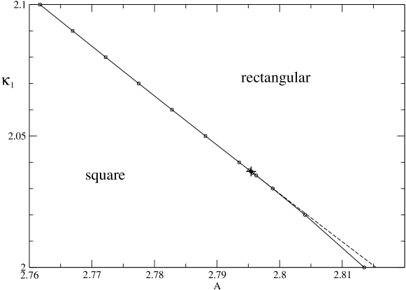
Figure 7: Phase diagram of the Yukawa-Coulomb model close to the tricritical point denoted by the cross. The critical line of second-order transitions is denoted by open squares, first-order transitions are indicated by open circles. The dashed line corresponds to an artificial prolongation of the critical line of second-order transitions to the region where first-order transitions are dominant.

The phase diagram of the Yukawa-Coulomb model is pictured in Fig. 7. The second-order transitions are marked by open squares, the first-order by open circles and the tricritical point by the cross. The dashed line is an artificial prolongation of the critical line beyond the tricritical point.

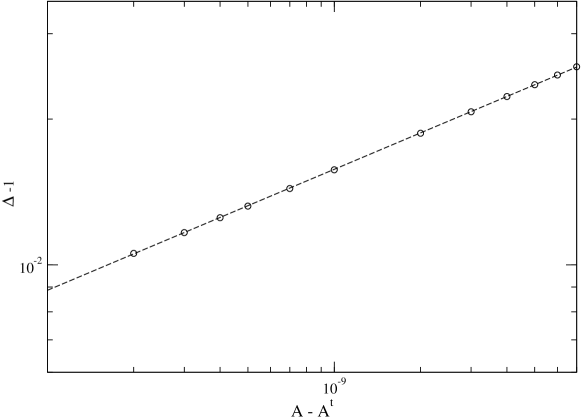
Figure 8: The plot of the deviation $\Delta-1$ versus $A-A^{t}$ for the Yukawa-Coulomb model close to the tricritical point.

In Fig. 8, $\Delta-1$ is plotted as the function of $(A-A^{t})$ in order to check the tricritical exponent in the Yukawa-Coulomb case. The numerical data are represented by open circles. Fitting the log-log plot via $\Delta-1\propto(A-A^{t})^{\beta^{t}}$, represented by the dashed line, yields the tricritical exponent $\beta^{t}=0.2498$ which is very close to the anticipated mean-field one $\beta^{t}=1/4$.

References

- [1] R. Bausch, Ginzburg criterion for tricritical points, Z. Physik 254 (1972) 81–88.
- [2] S. Bernstein, Sur les fonctions absolument monotones, Acta Math. 52 (1929) 1–66.
- [3] L. Bétermin and P. Zhang, Minimization of energy per particle among Bravais lattices in the whole plane: Lennard-Jones and Thomas-Fermi cases, Commun. Contemp. Math. 17 (2015) 1450049.
- [4] L. Bétermin, Two-dimensional theta functions and crystallization among Bravais lattices, SIAM J. Math. Anal. 48 (2016) 3236–3269.
- [5] L. Bétermin, Local variational study of 2d lattice energies and application to Lennard-Jones type interactions, Nonlinearity 31 (2018) 3973–4005.
- [6] L. Bétermin and M. Petrache, Optimal and non-optimal lattices for non-completely monotone interaction potentials, Anal. Math. Phys. 9 (2019) 2033–-2073.
- [7] L. Bétermin, Theta functions and optimal lattices for a grid cells model, SIAM J. Appl. Math. 81 (2021) 1931–1953.
- [8] L. Bétermin, L. De Luca and M. Petrache, Crystallization to the square lattice for a two-body potential. Arch. Ration. Mech. Anal. 240 (2021) 987–1053.
- [9] L. Bétermin, M. Friedrich and U. Stefanelli, Lattice ground states for embedded-atom models in 2D and 3D, Lett. Math. Phys. 111 (2021) 107.
- [10] L. Bétermin, Effect of periodic arrays of defects on lattice energy minimizers, Ann. Henri Poincaré 22 (2021) 2995–3023.
- [11] L. Bétermin, L. Šamaj and I. Travěnec, Three-dimensional lattice ground states for Riesz and Lennard-Jones type energies, Stud. Appl. Math. 150 (2023) 69–91.
- [12] L. Bétermin, Optimality of the triangular lattice for Lennard-Jones type lattice energies: a computer assisted method, J. Phys. A: Math. Theor. 56 (2023) 145204.
- [13] X. Blanc and M. Lewin, The crystallization conjecture: a review, EMS Surv. Math. Sci. 2 (2015) 255–306.
- [14] H. Cohn and A. Kumar, Universally optimal distribution of points on spheres. J. Amer. Math. Soc. 20 (2007) 99–148.
- [15] H. Cohn, A. Kumar, S.D. Miller, D. Radchenko, and M. Viazovska, The sphere packing problem in dimension 24, Ann. Math. 185 (2017) 1017–1033.
- [16] H. Cohn, A. Kumar, S.D. Miller, D. Radchenko, and M. Viazovska, Universal optimality of the and Leech lattices and interpolation formulas, Ann. Math. 196 (2022) 983–1082.
- [17] M. Faulhuber and S. Steinerberger, Optimal Gabor frame bounds for separable lattices and estimates for Jacobi theta functions, J. Math. Anal. Appl. 445 (2017) 407–-422.
- [18] I.S. Gradshteyn and I.M. Ryzhik, Table of Integrals, Series, and Products, 6th edn., Academic Press, London, 2000.
- [19] I.G. Kaplan, Intermolecular Interactions: Physical Picture, Computational Methods, Model Potentials, John Wiley and Sons, New York, 2006.
- [20] L.D. Landau, On the theory of phase transitions, Zh. Eksp. Teor. Fiz. 7 (1937) 19–32.
- [21] L.D. Landau and E.M. Lifshitz, Course of Theoretical Physics Vol. 5: Statistical Physics, 3rd edn., Elsevier, Amsterdam, 1980.
- [22] S. Luo, X. Ren and J. Wei, Non-hexagonal lattices from a two species interacting system, SIAM J. Math. Anal. 52 (2020) 1903–-1942.
- [23] S. Luo and J. Wei, On minima of sum of theta functions and Mueller-Ho Conjecture, Arch. Ration. Mech. Anal. 243 (2022) 139–-199.
- [24] S. Luo and J. Wei, On minima of difference of Epstein zeta functions and exact solutions to Lennard-Jones lattice energy, preprint, arXiv:2212.10727 (2022).
- [25] S. Luo and J. Wei, On lattice hexagonal crystallization for non-monotone potentials, preprint, arXiv:2302.05042 (2023).
- [26] A. Mogilner, L. Edelstein-Keshet, L. Bent, and A. Spiros, Mutual interactions, potentials, and individual distance in a social aggregation, J. Math. Biol 47 (2003) 353–389.
- [27] H.L. Montgomery, Minimal theta functions, Glasg. Math. J. 30 (1988) 75–85.
- [28] E. Sandier and S. Serfaty, From the Ginzburg-Landau model to vortex lattice problems. Comm. Math. Phys. 313 (2012) 635–743.
- [29] L. Šamaj, Z. Bajnok, Introduction to the Statistical Physics of Integrable Many-body Systems, Cambridge University Press, Cambridge, 2013.
- [30] J.C. Tolédano and P. Tolédano, The Landau theory of phase transitions, World Scientific, Singapore, 1987.
- [31] I. Travěnec and L. Šamaj, Two-dimensional Wigner crystals of classical Lennard-Jones particles, J. Phys. A: Math. Theor. 52 (2019) 205002.
- [32] I. Travěnec and L. Šamaj, Generation of off-critical zeros for hypercubic Epstein zeta functions, Appl. Math. Comput. 413 (2022) 126611.
- [33] M. Viazovska, The sphere packing problem in dimension 8, Ann. Math. 185 (2017) 991–1015.