Cosmic Riddles: Unraveling the Influence of Cosmic Curvature and Dark Energy Perturbations on Large-Scale Structure Formation - Part I

Abstract

This study explores the impact of cosmic curvature on structure formation through general relativistic first-order perturbation theory, focusing on scalar fluctuations and excluding anisotropic stress sources. We analyze continuity and Euler equations, incorporating cosmic curvature into Einstein equations. Emphasizing late-time dynamics, we investigate matter density contrast evolution in the presence of cosmic curvature and dark energy perturbations, with a specific focus on sub-Hubble scales. Solving the evolution equation, we conduct data analysis using cosmic chronometers, baryon acoustic oscillations, type Ia supernova observations, and $f\sigma_{8}$ data. While constraints on certain parameters remain consistent, excluding cosmic curvature tightens constraints on $\Omega_{\rm m0}$ and $\sigma_{\rm 80}$ in $\Lambda$CDM and wCDM models. Intriguingly, the non-phantom behavior of dark energy proves more favorable in both wCDM and CPL models across diverse data combinations.

1 Introduction

The investigation into the late-time cosmic dynamics, propelled by observations like type Ia supernovae [1, 2, 3, 4, 5, 6, 7, 8], cosmic microwave background [9, 10, 11], baryon acoustic oscillations [12, 13, 14], and cosmic chronometers [15, 16, 17], has unequivocally established the accelerating expansion of our Universe. This cosmic phenomenon, however, eludes conventional explanations within the confines of standard matter or dark matter paradigms governed by general relativity. Consequently, two overarching theoretical avenues have emerged to decipher the enigma of late-time cosmic acceleration: the proposition of dark energy [18, 19, 20, 21, 22, 23] or the contemplation of modifications to the foundational framework of general relativity [24, 25, 26, 27, 28, 29, 30, 31, 32, 33, 34, 35, 36]. While dark energy postulates an entity with a substantial negative pressure, capable of driving the cosmic acceleration, alternative theories entertain the prospect of tweaking the fundamental tenets of general relativity to account for the observed cosmic dynamics. This dual spectrum of theoretical paradigms underscores the intricate interplay between cosmic constituents and gravitational theories in unraveling the mysteries of the cosmos.

Dark energy, characterized by its significant negative pressure, emerges as a viable explanation for the observed late-time cosmic acceleration. While a plethora of theoretical models addressing dark energy populate the literature, the $\Lambda$CDM model stands out as a frontrunner in success [37]. This model attributes the role of dark energy to the cosmological constant ($\Lambda$), with a constant equation of state, denoted as $-1$. Despite its success, the $\Lambda$CDM model grapples with theoretical conundrums such as the cosmic coincidence and fine-tuning problems [38, 39, 40, 41]. Moreover, observational tensions, including the Hubble tension [42, 43, 44, 45] and $\sigma_{8}$ (or $S_{8}$) discrepancies [46, 47, 48, 49], underscored by variations in the measured values of $H_{0}$ and $\sigma_{\rm 80}$ between early and late universe observations, impel the quest to transcend the limitations of the $\Lambda$CDM model. This necessitates delving into alternative frameworks that can offer more comprehensive and accurate insights into the cosmic dynamics at play.

The conventional $\Lambda$CDM model operates under the assumption that the 3-space of the four-dimensional space-time is flat [9, 10, 11]. However, one avenue to transcend the standard $\Lambda$CDM model involves incorporating the influence of cosmic curvature into our analysis. While literature acknowledges prior investigations exploring the prospect of non-zero cosmic curvature in the Universe [50, 51, 52, 53, 54, 55, 56, 57, 58, 59, 60, 61, 62, 63, 64, 65, 66, 67, 68, 69], these studies predominantly focus on correcting the background dynamics of cosmic expansion due to the introduction of non-zero spatial curvature. Yet, the imperative lies in comprehensively examining the impact of cosmic curvature on the evolution of perturbations [70]. In this study, we go beyond the conventional approach by not only considering the effect of cosmic curvature on background dynamics but also delving into its role in shaping the evolution of first-order perturbations. This exploration involves crucial quantities like the matter density contrast and the growth rate, providing a more nuanced understanding of the interplay between cosmic curvature and perturbation dynamics.

The potential degeneracies between the equation of state for dark energy and cosmic curvature necessitate a comprehensive exploration of alternative dark energy models [71, 72, 73, 74, 75]. In our study, we go beyond the standard constant equation of state in the $\Lambda$CDM model and delve into models where the equation of state varies. Specifically, we consider the wCDM and the Chevallier-Polarski-Linder (CPL) [76, 77] model. The wCDM model features a dark energy equation of state that remains static over time but can take various values, including the cosmological constant’s value of $-1$. On the other hand, the CPL model introduces dynamic variations in the equation of state of dark energy. By adopting these models, we aim to scrutinize the potential degeneracies between the equation of state for dark energy and cosmic curvature, providing a more nuanced understanding of their interplay and its implications for cosmological dynamics.

While prevailing literature often assumes the homogeneity of dark energy, particularly evident in the $\Lambda$CDM model where dark energy exhibits no fluctuations, our study takes a pioneering approach. We extend our analysis beyond the homogeneous paradigm to encompass scenarios where dark energy experiences perturbations. This departure from the conventional assumptions is not only relevant for the $\Lambda$CDM model but also extends to other models like the wCDM and CPL [78, 79, 80, 81, 82]. A pivotal aspect of our investigation involves assessing the potential impact of dark energy fluctuations on the intricate process of structure formation. To accomplish this, we develop a robust mathematical framework that integrates dark energy perturbations within the realm of first-order fluctuations and general relativistic perturbations. It is essential to note that while the theoretical groundwork is laid out in this part of the study, the actual data analysis, focusing on realistic dark energy models featuring fluctuations, will be elucidated in the subsequent section of our research.

This paper unfolds in a structured manner. Section 2 delves into the metric employed for first-order perturbation theory, focusing on scalar fluctuations and excluding anisotropic stress. Moving to Section 3, we compute the background and first-order Einstein tensor components within this metric. The evolution of the perfect fluid in both background and first-order perturbation, including velocity fields, energy-momentum tensor, continuity, and Euler equations, is detailed in Section 4. Section 5 concentrates on treating matter as a perfect fluid, deriving continuity and Euler equations, and establishing a differential equation for the matter density contrast. Late-time dynamics, exploring background expansion and scalar perturbation evolution with matter and dark energy as Universe constituents, take center stage in Section 6. Section 7 reformulates all evolution equations in the sub-Hubble limit for computational simplicity and to extract relevant perturbation quantities like the growth rate. The four observational datasets considered in the analysis are briefly outlined in Section 8. Section 9 delves into the main study findings. Finally, Section 10 encapsulates the conclusion.

2 The metric to describe background and first order scalar fluctuations

We adopt the conformal Newtonian gauge to elucidate first-order general relativistic perturbations. Within this gauge, the line element, denoted as $d_{s}$, characterizing solely scalar fluctuations, is expressed as

$$d_{s}^{2}=\sigma\left[-c^{2}(1+2\Phi)dt^{2}+a^{2}(1-2\Phi)\left(\frac{dr^{2}}{1-\kappa r^{2}}+r^{2}d\theta^{2}+r^{2}\sin^{2}\theta d\phi^{2}\right)\right],$$ (2.1)

where $t$ represents cosmic time, $r$ denotes the comoving radial coordinate, and $\theta$ and $\phi$ stand for the comoving polar and azimuthal angles, respectively. $\kappa$ signifies the curvature of the space-time, while $c$ is the speed of light in a vacuum and $a$ is the cosmic scale factor. The Bardeen potential is denoted as $\Phi$, and the parameter $\sigma$ is introduced to characterize the signature of the metric in the line element, defined as

$$\sigma=\begin{cases}+1,&\mbox{for }(-,+,+,+)\mbox{ signature},\\ -1,&\mbox{for }(+,-,-,-)\mbox{ signature}.\\ \end{cases}$$ (2.2)

Note that in the line element given by Eq. (2.1), we adopt the scalar-vector-tensor decomposition theory. This allows us to analyze scalar fluctuations independently. Additionally, our assumption of the absence of anisotropic stresses in the Universe streamlines calculations, enabling us to focus on a single degree of freedom in the scalar fluctuations, governed by the Bardeen potential $\Phi$. A background metric, representing the Friedmann-Lemaître-Robertson-Walker (FLRW) metric with curvature contributions, is characterized by $\Phi=0$.

The metric and its inverse can be expressed perturbatively as follows

$$g_{\mu\nu} = \bar{g}_{\mu\nu}+\delta g_{\mu\nu},$$ (2.3)

$$g^{\mu\nu} = \bar{g}^{\mu\nu}+\delta g^{\mu\nu},$$ (2.4)

respectively. We denote the background counterpart of a quantity with an over bar, and its first-order perturbation with the pre-factor $\delta$. Consistent notation is maintained throughout this study. The non-zero components of both the background metric and its inverse are listed below:

$$\bar{g}_{tt} = -\sigma c^{2},\hskip 28.45274pt\bar{g}_{rr}=\frac{\sigma a^{2}}{1-\kappa r^{2}},\hskip 28.45274pt\bar{g}_{\theta\theta}=\sigma a^{2}r^{2},\hskip 28.45274pt\bar{g}_{\phi\phi}=\sigma a^{2}r^{2}\sin^{2}\theta,$$ (2.5)

$$\bar{g}^{tt} = -\frac{\sigma}{c^{2}},\hskip 28.45274pt\bar{g}^{rr}=\frac{\sigma(1-\kappa r^{2})}{a^{2}},\hskip 28.45274pt\bar{g}^{\theta\theta}=\frac{\sigma}{a^{2}r^{2}},\hskip 28.45274pt\bar{g}^{\phi\phi}=\frac{\sigma}{a^{2}r^{2}\sin^{2}\theta}.$$ (2.6)

The non-zero components of the first-order metric and its inverse are listed below:

$$\delta g_{tt} = -2\sigma c^{2}\Phi,\hskip 5.69046pt\delta g_{rr}=-\frac{2\sigma a^{2}\Phi}{1-\kappa r^{2}},\hskip 5.69046pt\delta g_{\theta\theta}=-2\sigma a^{2}r^{2}\Phi,\hskip 5.69046pt\delta g_{\phi\phi}=-2\sigma a^{2}r^{2}\left(\sin^{2}\theta\right)\Phi,$$ (2.7)

$$\delta g^{tt} = \frac{2\sigma\Phi}{c^{2}},\hskip 14.22636pt\delta g^{rr}=\frac{2\sigma(1-\kappa r^{2})\Phi}{a^{2}},\hskip 14.22636pt\delta g^{\theta\theta}=\frac{2\sigma\Phi}{a^{2}r^{2}},\hskip 14.22636pt\delta g^{\phi\phi}=\frac{2\sigma\Phi}{a^{2}r^{2}\sin^{2}\theta}.$$ (2.8)

3 The background and the first order Einstein tensor

With the components of the metric and its inverse in hand, we proceed to compute the components of the Einstein tensor perturbatively, denoted as

$$G^{\mu}_{\nu}=\bar{G}^{\mu}_{\nu}+\delta G^{\mu}_{\nu}.$$ (3.1)

The non-zero components of the Einstein tensor are provided below:

$$\bar{G}^{t}_{t} = -3\sigma\left(\frac{H^{2}}{c^{2}}+\frac{\kappa}{a^{2}}\right),$$ (3.2)

$$\bar{G}^{r}_{r} = \bar{G}^{\theta}_{\theta}=\bar{G}^{\phi}_{\phi}=-\sigma\left(\frac{2\dot{H}+3H^{2}}{c^{2}}+\frac{\kappa}{a^{2}}\right),$$ (3.3)

Where an over dot on a quantity indicates the partial derivative of that quantity with respect to cosmic time $t$. It’s important to note that for background quantities, the partial derivative with respect to $t$ is equivalent to the total derivative with respect to $t$, since all background quantities are functions of cosmic time $t$. On the other hand, perturbed quantities are functions of all four coordinates—$t$, $r$, $\theta$, and $\phi$. Here, $H$ represents the Hubble parameter, defined as $\frac{\dot{a}}{a}$. The $t$-$t$ component of the first-order Einstein tensor is expressed as

$$\delta G^{t}_{t}=2\sigma\left[\frac{3H\left(\frac{\partial\Phi}{\partial t}+H\Phi\right)}{c^{2}}-\frac{\vec{\nabla}^{2}\Phi+3\kappa\Phi}{a^{2}}\right],$$ (3.4)

where $\vec{\nabla}^{2}f$ represents the comoving gradient square, pertaining to the three-dimensional space, of a quantity $f$, and is defined as

$$\vec{\nabla}^{2}f = \frac{1}{h_{r}h_{\theta}h_{\phi}}\left[\frac{\partial}{\partial r}\left(\frac{h_{\theta}h_{\phi}}{h_{r}}\frac{\partial f}{\partial r}\right)+\frac{\partial}{\partial\theta}\left(\frac{h_{\phi}h_{r}}{h_{\theta}}\frac{\partial f}{\partial\theta}\right)+\frac{\partial}{\partial\phi}\left(\frac{h_{r}h_{\theta}}{h_{\phi}}\frac{\partial f}{\partial\phi}\right)\right],$$ (3.5)

$$= \frac{1}{r^{2}}\left[r^{2}(1-\kappa r^{2})\frac{\partial^{2}v}{\partial r^{2}}+r(2-3\kappa r^{2})\frac{\partial f}{\partial r}+\frac{\partial^{2}v}{\partial\theta^{2}}+\left(\cot\theta\right)\frac{\partial f}{\partial\theta}+\frac{\frac{\partial^{2}f}{\partial\phi^{2}}}{\sin^{2}\theta}\right].$$

Here, the factors of the curvilinear coordinates are given as

$$h_{r} = \frac{1}{\sqrt{1-\kappa r^{2}}},$$

$$h_{\theta} = r,$$

$$h_{\phi} = r\sin\theta.$$ (3.6)

The $r$-$t$ and $t$-$r$ components of the first-order Einstein tensor are given as

$$\delta G^{r}_{t}=\frac{2\sigma(1-\kappa r^{2})}{a^{2}}\frac{\partial}{\partial r}\left(\frac{\partial\Phi}{\partial t}+H\Phi\right)=-\frac{c^{2}(1-\kappa r^{2})}{a^{2}}\delta G^{t}_{r}.$$ (3.7)

The $\theta$-$t$ and $t$-$\theta$ components of the first-order Einstein tensor are given as

$$\delta G^{\theta}_{t}=\frac{2\sigma}{a^{2}r^{2}}\frac{\partial}{\partial\theta}\left(\frac{\partial\Phi}{\partial t}+H\Phi\right)=-\frac{c^{2}}{a^{2}r^{2}}\delta G^{t}_{\theta}.$$ (3.8)

The $\phi$-$t$ and $t$-$\phi$ components of the first-order Einstein tensor are given as

$$\delta G^{\phi}_{t}=\frac{2\sigma}{a^{2}r^{2}\sin^{2}\theta}\frac{\partial}{\partial\phi}\left(\frac{\partial\Phi}{\partial t}+H\Phi\right)=-\frac{c^{2}}{a^{2}r^{2}\sin^{2}\theta}\delta G^{t}_{\phi}.$$ (3.9)

The $r$-$r$, $\theta$-$\theta$, and $\phi$-$\phi$ components of the first-order Einstein tensor are given as

$$\delta G^{r}_{r}=\delta G^{\theta}_{\theta}=\delta G^{\phi}_{\phi}=2\sigma\left[\frac{\frac{\partial^{2}\Phi}{\partial t^{2}}+4H\frac{\partial\Phi}{\partial t}+(2\dot{H}+3H^{2})\Phi}{c^{2}}-\frac{\kappa\Phi}{a^{2}}\right],$$ (3.10)

All other components of the first-order Einstein tensor are trivially zero.

4 The description of a perfect fluid

In this section, we elucidate the dynamics of a perfect fluid within this metric framework.

4.1 The background and the first order velocity field of a perfect fluid

To characterize a perfect fluid, let’s express its four-velocity components, both covariant and contravariant, perturbatively as

$$U^{\mu} = \bar{U}^{\mu}+\delta U^{\mu},$$ (4.1)

$$U_{\mu} = \bar{U}_{\mu}+\delta U_{\mu}.$$ (4.2)

The spatial components of the contravariant four-velocity become zero when studying only scalar fluctuations. Thus, we have

$$\bar{U}^{r}=\bar{U}^{\theta}=\bar{U}^{\phi}=0.$$ (4.3)

The time component of the contravariant four-velocity can be computed using the identity provided as

$$\bar{g}_{\mu\nu}\bar{U}^{\mu}\bar{U}^{\nu}=-\sigma c^{2}.$$ (4.4)

Applying the aforementioned identity, we derive an algebraic equation for $\bar{U}^{t}$ as

$$\left(\bar{U}^{t}\right)^{2}=1,$$ (4.5)

and we opt for the positive solution of the above equation, yielding

$$\bar{U}^{t}=1.$$ (4.6)

Utilizing the contruction with the background metric, i.e., $\bar{U}{\mu}=\bar{g}{\mu\nu}\bar{U}^{\nu}$, we obtain all components of the covariant four-velocity as

$$\bar{U}_{t}=-\sigma c^{2},\hskip 28.45274pt\bar{U}_{r}=\bar{U}_{\theta}=\bar{U}_{\phi}=0.$$ (4.7)

Similarly, the first-order time component of the contravariant four-vector is computed using the provided identity

$$g_{\mu\nu}U^{\mu}U^{\nu}=-\sigma c^{2}.$$ (4.8)

And we have

$$\delta U^{t}=-\Phi,$$ (4.9)

By using $U_{\mu}=g_{\mu\nu}U^{\nu}$, we get

$$\delta U_{t} = -\sigma c^{2}\Phi,$$ (4.10)

$$\delta U_{r} = \frac{\sigma a^{2}\delta U^{r}}{1-\kappa r^{2}},\hskip 5.69046pt\delta U_{\theta}=\sigma a^{2}r^{2}\delta U^{\theta},\hskip 5.69046pt\delta U_{\phi}=\sigma a^{2}r^{2}\left(\sin^{2}\theta\right)\delta U^{\phi},$$ (4.11)

The curl-free part of the velocity contributes to the scalar fluctuations. Therefore, we opt for

$$\delta U_{r}=-\sigma\frac{\partial(av)}{\partial r},\hskip 14.22636pt\delta U_{\theta}=-\sigma\frac{\partial(av)}{\partial\theta},\hskip 14.22636pt\delta U_{\phi}=-\sigma\frac{\partial(av)}{\partial\phi}.$$ (4.12)

Now, employing the relations in Eq. (4.11), we determine the contravariant spatial components of the four-velocity as

$$\delta U^{r}=-\frac{1-\kappa r^{2}}{a}\frac{\partial v}{\partial r},\hskip 14.22636pt\delta U^{\theta}=-\frac{1}{ar^{2}}\frac{\partial v}{\partial\theta},\hskip 14.22636pt\delta U^{\phi}=-\frac{1}{ar^{2}\sin^{2}\theta}\frac{\partial v}{\partial\phi}.$$ (4.13)

4.2 The energy-momentum tensor of a perfect fluid

The energy-momentum tensor of a perfect fluid can be expressed in the following form

$$T^{\mu}_{\nu}=\left(\rho+\frac{P}{c^{2}}\right)U^{\mu}U_{\nu}+\sigma P\delta^{\mu}_{\nu},$$ (4.14)

where $\rho$ and $P$ represent the volumetric mass density and pressure of the perfect fluid, respectively, while $\delta$ denotes the usual Kronecker delta symbol. These quantities are expressed in perturbative order as

$$\rho = \bar{\rho}+\delta\rho,$$ (4.15)

$$P = \bar{P}+\delta P.$$ (4.16)

Similarly, the energy-momentum tensor of the perfect fluid can be expressed in perturbative order as

$$T^{\mu}_{\nu}=\bar{T}^{\mu}_{\nu}+\delta T^{\mu}_{\nu},$$ (4.17)

Utilizing Eqs. (4.3),  (4.6),  (4.7),  (4.9),  (4.10),  (4.13),  (4.15), and (4.16) in Eq.(4.14), we obtain components of the energy-momentum tensor for both the background and first-order counterpart. The non-zero background components of the energy-momentum tensor for the perfect fluid are listed below

$$\bar{T}^{t}_{t} = -\sigma c^{2}\bar{\rho},$$ (4.18)

$$\bar{T}^{r}_{r} = \bar{T}^{\theta}_{\theta}=\bar{T}^{\phi}_{\phi}=\sigma\bar{P}.$$ (4.19)

The $t$-$t$ component of the first-order energy-momentum tensor for the perfect fluid is given below

$$\delta T^{t}_{t}=-\sigma c^{2}\delta\rho.$$ (4.20)

The $r$-$t$ and $t$-$r$ components of the first-order energy-momentum tensor for the perfect fluid are given below

$$\delta T^{r}_{t}=\frac{\sigma(1-\kappa r^{2})(c^{2}\bar{\rho}+\bar{P})\frac{\partial v}{\partial r}}{a}=-\frac{c^{2}(1-\kappa r^{2})}{a^{2}}\delta T^{t}_{r}.$$ (4.21)

The $\theta$-$t$ and $t$-$\theta$ components of the first-order energy-momentum tensor for the perfect fluid are given below

$$\delta T^{\theta}_{t}=\frac{\sigma(c^{2}\bar{\rho}+\bar{P})\frac{\partial v}{\partial\theta}}{ar^{2}}=-\frac{c^{2}}{a^{2}r^{2}}\delta T^{t}_{\theta}.$$ (4.22)

The $\phi$-$t$ and $t$-$\phi$ components of the first-order energy-momentum tensor for the perfect fluid are given below

$$\delta T^{\phi}_{t}=\frac{\sigma(c^{2}\bar{\rho}+\bar{P})\frac{\partial v}{\partial\phi}}{ar^{2}\sin^{2}\theta}=-\frac{c^{2}}{a^{2}r^{2}\sin^{2}\theta}\delta T^{t}_{\phi},$$ (4.23)

The $r$-$r$, $\theta$-$\theta$, and $\phi$-$\phi$ components of the first-order energy-momentum tensor for the perfect fluid are given below

$$\delta T^{r}_{r}=\delta T^{\theta}_{\theta}=\delta T^{\phi}_{\phi}=\sigma\delta P.$$ (4.24)

All other components of the first-order energy-momentum tensor for the perfect fluid are trivially zero.

4.3 The continuity equation for a perfect fluid

In this study, we assume that there is no interaction of the perfect fluid with other fields or fluids present in the universe. Therefore, the divergence of the energy-momentum tensor for the perfect fluid is zero, i.e.,

$$\nabla_{\mu}T^{\mu}_{\nu}=0.$$ (4.25)

Analyzing the above equation order by order, we arrive at the background condition

$$\bar{\nabla}_{\mu}\bar{T}^{\mu}_{\nu}=0.$$ (4.26)

The above condition corresponds to four equations. The $t$ part of this equation corresponds to

$$\dot{\bar{\rho}}+3H\left(\bar{\rho}+\frac{\bar{P}}{c^{2}}\right)=0.$$ (4.27)

This constitutes the continuity equation for the perfect fluid at the background level. Now, we establish a relationship between the background pressure and energy density of the perfect fluid using a quantity called the equation of state, denoted by $w$ and defined as

$$\bar{P}=w\bar{\rho}c^{2}.$$ (4.28)

Utilizing Eq.(4.28), Eq.(4.27) can be rewritten as

$$\dot{\bar{\rho}}+3H(1+w)\bar{\rho}=0.$$ (4.29)

Similarly, we obtain the continuity equation for the perfect fluid at the first order as

$$\dot{(\delta\rho)}+3H\left(\delta\rho+\frac{\delta P}{c^{2}}\right)-\frac{(1+w)\bar{\rho}(\theta_{g}+3a\dot{\Phi})}{a}=0,$$ (4.30)

where

$$\theta_{g}=\vec{\nabla}^{2}v=\frac{1}{r^{2}}\left[r^{2}(1-\kappa r^{2})\frac{\partial^{2}v}{\partial r^{2}}+r(2-3\kappa r^{2})\frac{\partial v}{\partial r}+\frac{\partial^{2}v}{\partial\theta^{2}}+\left(\cot\theta\right)\frac{\partial v}{\partial\theta}+\frac{\frac{\partial^{2}v}{\partial\phi^{2}}}{\sin^{2}\theta}\right].$$ (4.31)

Now, we define the density contrast, $\delta_{g}$, for the perfect fluid as

$$\delta\rho=\bar{\rho}\delta_{g}.$$ (4.32)

Applying the above definition, Eq.(4.30) can be rewritten as

$$\dot{\delta}_{g}-3wH\delta_{g}-\frac{(1+w)\theta_{g}}{a}-3(1+w)\dot{\Phi}+\frac{3H(\delta P)}{c^{2}\bar{\rho}}=0.$$ (4.33)

4.4 The Euler equations for a perfect fluid

The spatial parts of Eq.(4.25) are referred to as the Euler equations for the perfect fluid. The background Euler equations for the perfect fluid are trivially zero, i.e.,

$$\bar{\nabla}_{\mu}\bar{T}^{\mu}_{r}=\bar{\nabla}_{\mu}\bar{T}^{\mu}_{\theta}=\bar{\nabla}_{\mu}\bar{T}^{\mu}_{\phi}=0.$$ (4.34)

So, we do not obtain any corresponding equations. The first-order Euler equations corresponding to the conditions $\nabla_{\mu}T^{\mu}_{r}=0$, $\nabla_{\mu}T^{\mu}_{\theta}=0$, and $\nabla_{\mu}T^{\mu}_{\phi}=0$ are given as

$$\frac{\partial A}{\partial r} = 0,$$ (4.35)

$$\frac{\partial A}{\partial\theta} = 0,$$ (4.36)

$$\frac{\partial A}{\partial\phi} = 0,$$ (4.37)

respectively, where we have

$$A=\dot{v}+\left[(1-3w)H+\frac{\dot{w}}{1+w}\right]v-\frac{c^{2}\Phi}{a}-\frac{\delta P}{a(1+w)\bar{\rho}}.$$ (4.38)

As all three spatial first derivatives of $A$ are individually zero, we can further manipulate these equations into the following form to obtain a single useful Euler equation given as

$$\frac{1}{h_{r}h_{\theta}h_{\phi}}\left[\frac{\partial}{\partial r}\left(\frac{h_{\theta}h_{\phi}}{h_{r}}\frac{\partial A}{\partial r}\right)+\frac{\partial}{\partial\theta}\left(\frac{h_{\phi}h_{r}}{h_{\theta}}\frac{\partial A}{\partial\theta}\right)+\frac{\partial}{\partial\phi}\left(\frac{h_{r}h_{\theta}}{h_{\phi}}\frac{\partial A}{\partial\phi}\right)\right]=\vec{\nabla}^{2}A=0.$$ (4.39)

Finally, by substituting the expression of $A$ from Eq.(4.38) into Eq.(4.39), we obtain a simplified form of the Euler equation for the perfect fluid given as

$$\dot{\theta}_{g}+\left[(1-3w)H+\frac{\dot{w}}{1+w}\right]\theta_{g}-\frac{c^{2}\vec{\nabla}^{2}\Phi}{a}-\frac{\vec{\nabla}^{2}(\delta P)}{a(1+w)\bar{\rho}}=0.$$ (4.40)

5 Matter as a perfect fluid

The matter components of the Universe can be modeled as a perfect fluid. In this context, we assume the matter is cold, implying zero pressure and pressure perturbations, resulting in an equation of state $w=0$. Additionally, we assume that matter does not interact with other fields. Since matter is considered a perfect fluid, all the equations describing a perfect fluid hold true for matter, with the additional constraints $w=0$, $\bar{P}=0$, and $\delta P=0$. Moreover, $\dot{w}=0$ and $\vec{\nabla}^{2}(\delta P)=0$. Throughout this study, we denote all non-zero quantities related to matter with the subscript "m". Using these considerations, let’s outline the key equations for the matter counterpart. By substituting $w=0$ into Eq.(4.29), we obtain the background continuity equation for matter given as

$$\dot{\bar{\rho}}_{m}+3H\bar{\rho}_{m}=0.$$ (5.1)

Similarly, substituting $w=0$ and $\delta P=0$ into Eq.(4.33), we derive the first-order continuity equation for matter given as

$$\dot{\delta}_{m}-\frac{\theta_{m}}{a}-3\dot{\Phi}=0.$$ (5.2)

Similarly, substituting $w=0$, $\dot{w}=0$, and $\vec{\nabla}^{2}(\delta P)=0$ into Eq.(4.40), we derive the first-order Euler equation for matter given as

$$\dot{\theta}_{m}+H\theta_{m}-\frac{c^{2}\vec{\nabla}^{2}\Phi}{a}=0.$$ (5.3)

Let’s further manipulate Eqs.(5.2) and (5.3) to derive a more useful differential equation for matter. To do this, we first take the time derivative of Eq.(5.2), resulting in

$$\ddot{\delta}_{m}-\frac{\dot{\theta}_{m}}{a}+\frac{H\theta_{m}}{a}-3\ddot{\Phi}=0.$$ (5.4)

By utilizing Eq.(5.3), we obtain

$$\dot{\theta}_{m}=\frac{c^{2}\vec{\nabla}^{2}\Phi}{a}-H\theta_{m}.$$ (5.5)

Substituting the above equation into Eq.(5.4), we obtain

$$\ddot{\delta}_{m}+\frac{2H\theta_{m}}{a}-\frac{c^{2}\vec{\nabla}^{2}\Phi}{a^{2}}-3\ddot{\Phi}=0.$$ (5.6)

By employing Eq.(5.2), we obtain

$$\theta_{m}=a(\dot{\delta}_{m}-3\dot{\Phi}).$$ (5.7)

Substituting the above equation into Eq.(5.6), we obtain a second-order differential equation for $\delta_{m}$ that is independent of $\theta_{m}$, given as

$$\ddot{\delta}_{m}+2H\delta_{m}-\frac{c^{2}\vec{\nabla}^{2}\Phi}{a^{2}}-6H\dot{\Phi}-3\ddot{\Phi}=0.$$ (5.8)

6 Late-time dynamics: Einstein equations

We are now at a stage to derive the Einstein equations. This study emphasizes the dynamics of the late-time Universe, where we can neglect the contribution from radiation. We exclusively consider matter and dark energy, where ’matter’ refers to cold dark matter and baryons combined. Henceforth, we use the abbreviation ’DE’ for dark energy and denote any quantity related to dark energy with the subscript ’Q’. In this scenario, the Einstein equations are obtained perturbatively as follows

$$G^{\mu}_{\nu} = \frac{8\pi G}{c^{4}}\left[T^{\mu}_{\nu}(\rm matter)+T^{\mu}_{\nu}(\rm DE)\right],$$ (6.1)

$$\bar{G}^{\mu}_{\nu} = \frac{8\pi G}{c^{4}}\left[\bar{T}^{\mu}_{\nu}(\rm matter)+\bar{T}^{\mu}_{\nu}(\rm DE)\right],$$ (6.2)

$$\delta G^{\mu}_{\nu} = \frac{8\pi G}{c^{4}}\left[\delta T^{\mu}_{\nu}(\rm matter)+\delta T^{\mu}_{\nu}(\rm DE)\right],$$ (6.3)

where $G$ represents Newton’s gravitational constant. Utilizing all the above equations, we finally obtain the two independent non-trivial Einstein equations for the background evolution, given below

$$3H^{2} = 8\pi G(\bar{\rho}_{m}+\bar{\rho}_{Q})-\frac{3c^{2}\kappa}{a^{2}},$$ (6.4)

$$2\dot{H}+3H^{2} = -\frac{8\pi G}{c^{2}}\bar{P}_{Q}-\frac{c^{2}\kappa}{a^{2}}.$$ (6.5)

The $t$-$t$ component of the first-order perturbation in the Einstein equations is given as

$$\frac{c^{2}\left(\vec{\nabla}^{2}\Phi+3\kappa\Phi\right)}{a^{2}}-3H(\dot{\Phi}+H\Phi)=4\pi G(\delta\rho_{m}+\delta\rho_{Q})=4\pi G(\bar{\rho}_{m}\delta_{m}+\bar{\rho}_{Q}\delta_{Q}).$$ (6.6)

The three independent equations corresponding to the $r$-$t$ (or $t$-$r$), $\theta$-$t$ (or $t$-$\theta$), and $\phi$-$t$ (or $t$-$\phi$) components of the first-order perturbation in the Einstein equations are given as

$$\frac{\partial B}{\partial r} = 0,$$ (6.7)

$$\frac{\partial B}{\partial\theta} = 0,$$ (6.8)

$$\frac{\partial B}{\partial\phi} = 0,$$ (6.9)

respectively, where we have

$$B=\dot{\Phi}+H\Phi-\frac{4\pi Ga}{c^{2}}\left[\bar{\rho}_{m}v_{m}+\bar{\rho}_{Q}(1+w_{Q})v_{Q}\right].$$ (6.10)

Eqs.(6.7), (6.8), and (6.9) can be manipulated to be written in a single equation, as

$$\frac{1}{h_{r}h_{\theta}h_{\phi}}\left[\frac{\partial}{\partial r}\left(\frac{h_{\theta}h_{\phi}}{h_{r}}\frac{\partial B}{\partial r}\right)+\frac{\partial}{\partial\theta}\left(\frac{h_{\phi}h_{r}}{h_{\theta}}\frac{\partial B}{\partial\theta}\right)+\frac{\partial}{\partial\phi}\left(\frac{h_{r}h_{\theta}}{h_{\phi}}\frac{\partial B}{\partial\phi}\right)\right]=\vec{\nabla}^{2}B=0.$$ (6.11)

Substituting the expression of $B$ from Eq.(6.10) into Eq.(6.11), we finally obtain a simplified form of all three Einstein equations in a useful single equation, as

$$c^{2}\vec{\nabla}^{2}(\dot{\Phi}+H\Phi)=4\pi Ga\left[\bar{\rho}_{m}\theta_{m}+\bar{\rho}_{Q}(1+w_{Q})\theta_{Q}\right].$$ (6.12)

Finally, a single independent equation from either the $r$-$r$, $\theta$-$\theta$, or $\phi$-$\phi$ components of the first-order perturbation in the Einstein equations is given as

$$\ddot{\Phi}+4H\dot{\Phi}+(2\dot{H}+3H^{2})\Phi-\frac{c^{2}\kappa\Phi}{a^{2}}=\frac{4\pi G}{c^{2}}\delta P_{Q}.$$ (6.13)

All other Einstein equations are trivially zero, so no additional equations arise.

7 Late-time dynamics: sub-Hubble approximation

We are now focusing on sub-Hubble scales to study the evolution of perturbations, particularly the matter density contrast. On sub-Hubble scales, we assume that the spatial derivatives of a quantity are significantly larger than its time derivative. Therefore, we can neglect the terms $H\dot{\Phi}$ and $\ddot{\Phi}$ compared to the term $\frac{c^{2}\vec{\nabla}^{2}\Phi}{a^{2}}$ in Eq.(5.8). Thus, in the sub-Hubble limit, Eq.(5.8) can be approximated as

$$\ddot{\delta}_{m}+2H\delta_{m}-\frac{c^{2}\vec{\nabla}^{2}\Phi}{a^{2}}\simeq 0.$$ (7.1)

Applying similar approximations, in the sub-Hubble limit, Eq.(6.6) can be approximated as

$$\frac{c^{2}\vec{\nabla}^{2}\Phi}{a^{2}}\simeq 4\pi G(\bar{\rho}_{m}\delta_{m}+\bar{\rho}_{Q}\delta_{Q}).$$ (7.2)

Now, by substituting Eq.(7.2) into Eq.(7.1), we obtain the evolution equation for the matter density contrast as

$$\ddot{\delta}_{m}+2H\delta_{m}\simeq 4\pi G(\bar{\rho}_{m}\delta_{m}+\bar{\rho}_{Q}\delta_{Q})=\frac{3}{2}H^{2}(\Omega_{m}\delta_{m}+\Omega_{Q}\delta_{Q}),$$ (7.3)

where we define the density parameters for curvature, matter, and dark energy as

$$\Omega_{k}=-\frac{c^{2}\kappa}{a^{2}H^{2}},\hskip 14.22636pt\Omega_{m}=\frac{8\pi G\bar{\rho}_{m}}{3H^{2}},\hskip 14.22636pt\Omega_{Q}=\frac{8\pi G\bar{\rho}_{Q}}{3H^{2}}=1-\Omega_{m}-\Omega_{k}.$$ (7.4)

respectively. In the above equation, the last equality is a manifestation of Eq.(6.4). Utilizing the above definitions and expressing the derivatives with respect to the e-fold, $N=\ln a$, Eq.(7.4) can be rewritten as

$$\frac{d^{2}\delta_{m}}{dN^{2}}+F\frac{d\delta_{m}}{dN}-\frac{3}{2}\left[\Omega_{m}\delta_{m}+(1-\Omega_{m}-\Omega_{k})\delta_{Q}\right]\simeq 0,$$ (7.5)

where we have

$$F=2+\frac{1}{H}\frac{dH}{dN}=2+\frac{\dot{H}}{H^{2}}=\frac{1}{2}\left[2-\Omega_{m}-\left(1+3w_{Q}\right)(1-\Omega_{m}-\Omega_{k})\right].$$ (7.6)

7.1 Homogeneous dark energy

In this study, we focus on the homogeneous dark energy models, where dark energy has no fluctuations. Later, in near future, in the next study, we shall considers models in which the dark energy is not homogeneous. In the homogeneous dark energy models, we have $\delta_{Q}=0$ and the evolution equation for the matter density contrast becomes

$$\frac{d^{2}\delta_{m}}{dN^{2}}+\frac{1}{2}\left[2-\Omega_{m}-\left(1+3w_{Q}\right)(1-\Omega_{m}-\Omega_{k})\right]\frac{d\delta_{m}}{dN}-\frac{3}{2}\Omega_{m}\delta_{m}\simeq 0.$$ (7.7)

Additionally, by solving Eq.(5.1) and employing the definitions in Eq.(7.4), we obtain

$$\Omega_{m}=\frac{\Omega_{\rm m0}a^{-3}}{E^{2}}=\frac{\Omega_{\rm m0}e^{-3N}}{E^{2}}=\frac{\Omega_{\rm m0}(1+z)^{3}}{E^{2}},$$ (7.8)

where $E$ denotes the normalized Hubble parameter, defined as $E=\frac{H}{H_{0}}$, where $H_{0}$ represents the present value of the Hubble parameter. $\Omega_{\rm m0}$ represents the present value of the matter density contrast. $z$ represents the redshift and is related to the scale factor as $1+z=\frac{1}{a}$. The definition of $\Omega_{k}$ in Eq.(7.4) can be manipulated to be rewritten as

$$\Omega_{k}=\frac{\Omega_{\rm k0}a^{-2}}{E^{2}}=\frac{\Omega_{\rm k0}e^{-2N}}{E^{2}}=\frac{\Omega_{\rm k0}(1+z)^{2}}{E^{2}},$$ (7.9)

where $\Omega_{\rm k0}$ denotes the present value of the curvature density contrast. By employing Eqs.(7.8) and (7.9), along with the background Einstein equation Eq.(6.4), the normalized Hubble parameter $E$ can be expressed as

$$E^{2}=\Omega_{\rm m0}(1+z)^{3}+\Omega_{\rm k0}(1+z)^{2}+(1-\Omega_{\rm m0}-\Omega_{\rm k0})f_{\rm DE},$$ (7.10)

where $f_{\rm DE}$ is connected to the evolution of dark energy density and can be computed from the expression of the equation of state of dark energy, $w_{Q}$, as given below

$$f_{\rm DE}=\exp\left[3\int_{0}^{z}\frac{1+w_{Q}(\tilde{z})}{1+\tilde{z}}d\tilde{z}\right],$$ (7.11)

where $\tilde{z}$ serves as the dummy variable for the redshift $z$. In this study, we exclusively focus on three prominent dark energy models, namely the parametrizations of the equation of state of dark energy $w_{Q}$: the $\Lambda$CDM model, the wCDM parametrization, and the Chevallier-Polarski-Linder (CPL) parametrization [76, 77]. In these parametrizations, the equation of state for dark energy is expressed as

$$w_{Q}\hskip 2.84544pt(\text{$\Lambda$CDM}) = -1,$$ (7.12)

$$w_{Q}\hskip 2.84544pt(\text{wCDM}) = w_{0},$$ (7.13)

$$w_{Q}\hskip 2.84544pt(\text{CPL}) = w_{0}+w_{a}\frac{z}{1+z},$$ (7.14)

respectively, where $w_{0}$ serves as the model parameter for the wCDM model, while $w_{0}$ and $w_{a}$ are the two model parameters for the CPL parametrization. Therefore, the wCDM model is a subset of the CPL model where $w_{a}=0$. The $\Lambda$CDM model is a subset of the CPL model where $w_{0}=-1$ and $w_{a}=0$, and it is also a subset of the wCDM model where $w_{0}=-1$. By substituting Eqs.(7.12), (7.13), and (7.14) into Eq.(7.11), we obtain the expressions of $f_{\rm DE}$ for the $\Lambda$CDM, the wCDM, and the CPL models

$$f_{\rm DE}\hskip 2.84544pt(\text{$\Lambda$CDM}) = 1,$$ (7.15)

$$f_{\rm DE}\hskip 2.84544pt(\text{wCDM}) = (1+z)^{3(1+w_{0})},$$ (7.16)

$$f_{\rm DE}\hskip 2.84544pt(\text{CPL}) = (1+z)^{3(1+w_{0}+w_{a})}e^{-3w_{a}\frac{z}{1+z}},$$ (7.17)

respectively.

7.2 Initial conditions

We consider initial conditions in the early matter-dominated era to solve the differential equation in Eq.(7.7) at an initial redshift $z^{i}=1100$. We denote the initial value of any quantity by superscript "i". In the matter-dominated era, we approximately have $\Omega_{m}\simeq 1$, $\Omega_{k}\simeq 0$, and $\Omega_{Q}\simeq 0$. With these approximations, the evolution equation for $\delta_{m}$ during the matter-dominated era becomes

$$\frac{d^{2}\delta_{m}}{dN^{2}}+\frac{1}{2}\frac{d\delta_{m}}{dN}-\frac{3}{2}\delta_{m}\simeq 0\hskip 14.22636pt\text{(at early matter dominated era)}.$$ (7.18)

There are two solutions to the above differential equation. One is proportional to $a^{-3/2}$, representing the decaying solution. The other is the growing solution, corresponding to $\delta_{m}\propto a$. As we are interested in the growing mode solutions, we set the initial conditions accordingly as

$$\delta_{m}^{i} = a^{i},$$ (7.19)

$$\left(\frac{d\delta_{m}}{dN}\right)^{i} = a^{i}.$$ (7.20)

7.3 $f$ and $\sigma_{8}$

We are now turning our attention to two additional quantities. The first one is the logarithmic growth factor, defined as [83]

$$f=\frac{d\ln D_{+}}{d\ln a},$$ (7.21)

where $D_{+}$ represents the growing mode solution of the matter density contrast, $\delta_{m}$. In the sub-Hubble limit within this framework, the normalization factor of the matter power spectrum, denoted as $\sigma_{8}$, retains its scale-independence and can be represented as [84]

$$\sigma_{8}(z)=\sigma_{\rm 80}\frac{D_{+}(z)}{D_{+}(z=0)},$$ (7.22)

where $\sigma_{\rm 80}$ denotes the present value of $\sigma_{8}$.

8 Observational data

In our analysis, we incorporate diverse observational datasets to robustly constrain the model parameters and cosmological nuisance parameters. Our primary source of information comes from the Pantheon compilation, which compiles type Ia supernova observations. These supernovae serve as standard candles, and their apparent peak absolute magnitudes vary with redshift [7]. The observed apparent magnitude is dependent on both the luminosity of the source at a given redshift and the nuisance parameter $M_{B}$, representing the peak absolute magnitude of a type Ia supernova. We additionally take into account the covariances existing between data points at varying redshifts. To ensure a comprehensive analysis, we label this dataset as ’SN’.

In our exploration, we integrate data from cosmic chronometer (CC) observations, which encompasses an extensive collection of 32 Hubble parameter measurements spanning a diverse range of redshift values ($0.07\leq z\leq 1.965$). This dataset, meticulously detailed in [17], emerges as a pivotal asset in deciphering the complexities of cosmic evolution. It is noteworthy that within these 32 Hubble parameter measurements, 15 display correlations, a nuanced aspect we deliberately incorporate into our analytical framework. By judiciously considering these covariances, we elevate the precision of our analysis, ensuring a more nuanced understanding of the intricate dynamics governing the cosmic landscape. We denote this dataset as ’CC’.

Expanding our observational repertoire, we integrate baryon acoustic oscillations (BAO) data into our analysis. These observations provide insights into cosmological distances, specifically the angular diameter distance. The BAO dataset includes measurements in both the line of sight and transverse directions [13]. The former is connected to the Hubble parameter, while the latter is linked to the angular diameter distance [12, 13, 14]. Adhering to the methodology in [13], with the exception of eBOSS emission-line galaxies (ELGs) data at $z=0.8$ due to asymmetric statistical measurement deviations, we label the BAO observations as ’BAO’. Notably, BAO measurements are sensitive to the parameter $r_{d}$, representing the distance to the baryon drag epoch. We treat $r_{d}$ as a nuisance parameter in our analysis.

Finally, we incorporate $f\sigma_{8}$ data, spanning redshifts from $z=0.001$ to $z=1.944$, to constrain the model parameters across both background and perturbation evolutions [85]. This dataset is labeled ’$f\sigma_{8}$.’

By synthesizing information from these diverse observations, we aim to refine our understanding of the Universe’s dynamics, simultaneously constraining model parameters and accounting for relevant cosmological nuisance parameters.

9 Results

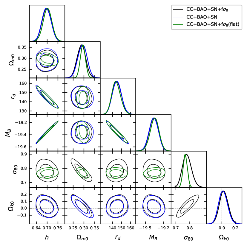
Figure 1: Constraints on the parameters of the $\Lambda$CDM model are depicted through various lines. The black, blue, and green lines correspond to the datasets combinations ’CC+BAO+SN+$f\sigma_{8}$’ (considering cosmic curvature), ’CC+BAO+SN’ (considering cosmic curvature), and ’CC+BAO+SN+$f\sigma_{8}$(flat)’ (excluding cosmic curvature), respectively.

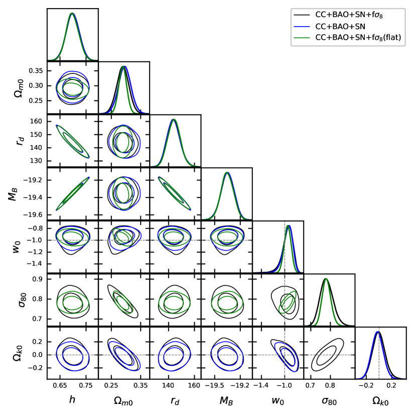
Figure 2: The constraints on the parameters of the wCDM model are illustrated through different lines. The black, blue, and green lines correspond to the datasets combinations ’CC+BAO+SN+$f\sigma_{8}$’ (accounting for cosmic curvature), ’CC+BAO+SN’ (factoring in cosmic curvature), and ’CC+BAO+SN+$f\sigma_{8}$(flat)’ (disregarding cosmic curvature), respectively.

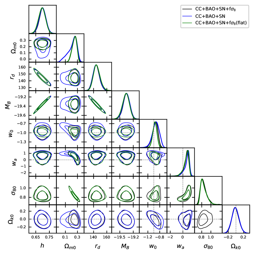
Figure 3: The constraints on the parameters of the CPL model are depicted through various lines. The black, blue, and green lines correspond to the datasets combinations ’CC+BAO+SN+$f\sigma_{8}$’ (considering cosmic curvature), ’CC+BAO+SN’ (accounting for cosmic curvature), and ’CC+BAO+SN+$f\sigma_{8}$(flat)’ (ignoring cosmic curvature), respectively.

Using the aforementioned observational data, we constrain all the model parameters in all three dark energy models. In Figure 1, a triangle plot is presented to display the confidence contours of each pair of parameters and the marginal probability plots for each parameter in the $\Lambda$CDM model. The black lines represent the ’CC+BAO+SN+$f\sigma_{8}$’ combination of the dataset, where cosmic curvature is taken into account in the analysis. The blue lines correspond to the ’CC+BAO+SN’ combination of the dataset, incorporating cosmic curvature. The green lines depict the ’CC+BAO+SN+$f\sigma_{8}$’ combination of the dataset, but in this case, cosmic curvature is not considered in the analysis (i.e., $\Omega_{\rm k0}=0$). The same color combinations are maintained for the same cases in the other two figures.

It is noteworthy that in all the figures, a quantity $h$ is considered, which is related to $H_{0}$ and given as

$$H_{0}=100\hskip 5.69046pth\hskip 5.69046pt\text{km}\hskip 2.84544pt\text{s}^{-1}\hskip 2.84544pt\text{Mpc}^{-1}.$$ (9.1)

Parameters	CC+BAO+SN+$f\sigma_{8}$	CC+BAO+SN	CC+BAO+SN+$f\sigma_{8}$(flat)
$h$	$0.698\pm 0.025$	$0.696\pm 0.025$	$0.702\pm 0.024$
$\Omega_{\rm m0}$	$0.288\pm 0.020$	$0.293\pm 0.021$	$0.295\pm 0.012$
$r_{d}$	$144.7\pm 5.0$	$144.9\pm 5.0$	$144.1^{+4.4}_{-5.2}$
$M_{B}$	$-19.359\pm 0.076$	$-19.362\pm 0.076$	$-19.348\pm 0.075$
$\sigma_{\rm 80}$	$0.781^{+0.029}_{-0.035}$	$-$	$0.767\pm 0.016$
$\Omega_{\rm k0}$	$0.030\pm 0.065$	$0.018^{+0.061}_{-0.068}$	$-$

Table 1: 1$\sigma$ bounds on the parameters of the $\Lambda$CDM model corresponding to three different combinations of datasets mentioned in the table.

We present all the marginalized 1$\sigma$ bounds on the parameters of the $\Lambda$CDM model in Table 1. Examining Figure 1 and Table 1, it is evident that the marginalized bounds on $h$, $r_{d}$, and $M_{B}$ remain similar in all three cases. This suggests that the inclusion of $f\sigma_{8}$ data or the consideration of cosmic curvature in the analysis does not significantly alter the constraints on these parameters.

The constraints on $\Omega_{\rm k0}$ also exhibit similarity between the ’CC+BAO+SN+$f\sigma_{8}$’ and ’CC+BAO+SN’ combinations. This implies that the inclusion of $f\sigma_{8}$ data does not lead to notable improvements in constraining the $\Omega_{\rm k0}$ parameter. Notably, interesting results emerge in the constraints on the $\Omega_{\rm m0}$ and $\sigma_{\rm 80}$ parameters. Constraints on $\Omega_{\rm m0}$ are similar for both ’CC+BAO+SN+$f\sigma_{8}$’ and ’CC+BAO+SN’ combinations but become notably tighter when cosmic curvature is excluded, i.e., for ’CC+BAO+SN+$f\sigma_{8}$(flat)’ (green line) combination. Similarly, the constraint on the $\sigma_{\rm 80}$ parameter is significantly tighter when the contribution of cosmic curvature is excluded. Furthermore, not only is the constraint tighter, but the mean value of $\sigma_{\rm 80}$ is higher when cosmic curvature is included in the analysis.

Parameters	CC+BAO+SN+$f\sigma_{8}$	CC+BAO+SN	CC+BAO+SN+$f\sigma_{8}$(flat)
$h$	$0.698\pm 0.025$	$0.699\pm 0.025$	$0.698\pm 0.025$
$\Omega_{\rm m0}$	$0.289\pm 0.021$	$0.295\pm 0.021$	$0.289\pm 0.014$
$r_{d}$	$144.1^{+4.6}_{-5.1}$	$143.9^{+4.6}_{-5.4}$	$144.3\pm 4.9$
$M_{B}$	$-19.350\pm 0.076$	$-19.350\pm 0.077$	$-19.353\pm 0.074$
$w_{0}$	$-0.956^{+0.11}_{-0.063}$	$-0.947^{+0.091}_{-0.064}$	$-0.950\pm 0.060$
$\sigma_{\rm 80}$	$0.781^{+0.030}_{-0.036}$	$-$	$0.781^{+0.021}_{-0.024}$
$\Omega_{\rm k0}$	$-0.004\pm 0.099$	$-0.025\pm 0.090$	$-$

Table 2: 1$\sigma$ bounds on the parameters of the wCDM model corresponding to three different combinations of datasets mentioned in the table.

In Figure 2, we present triangle plots illustrating the wCDM model parameters for the same combinations of datasets, maintaining consistent color codes as in Figure 1. Corresponding 1$\sigma$ bounds on the wCDM model parameters are tabulated in Table 2. Notably, an additional parameter, $w_{0}$, is introduced compared to the $\Lambda$CDM model. Similar to the $\Lambda$CDM model, the bounds on $h$, $r_{d}$, and $M_{B}$ exhibit similarity across all three cases.

For $\Omega_{\rm m0}$ and $\sigma_{\rm 80}$ parameters, constraints are marginally tighter in the flat case compared to the non-flat cases, although not significantly so. An intriguing observation is found in the constraints on the $w_{0}$ parameter. The $\Lambda$CDM model, corresponding to $w_{0}=-1$, is almost 1$\sigma$ away from the mean values obtained in all three cases. Notably, the non-phantom behavior ($w_{0}>-1$) of dark energy appears more favorable compared to the phantom behavior ($w_{0}<-1$) in all three cases.

Parameters	CC+BAO+SN+$f\sigma_{8}$	CC+BAO+SN	CC+BAO+SN+$f\sigma_{8}$(flat)
$h$	$0.700\pm 0.024$	$0.699\pm 0.025$	$0.696\pm 0.025$
$\Omega_{\rm m0}$	$0.249^{+0.044}_{-0.034}$	$0.217^{+0.092}_{-0.043}$	$0.249^{+0.044}_{-0.032}$
$r_{d}$	$144.0^{+4.5}_{-5.1}$	$144.2^{+4.5}_{-5.3}$	$144.9^{+4.5}_{-5.5}$
$M_{B}$	$-19.353\pm 0.074$	$-19.355^{+0.078}_{-0.071}$	$-19.365^{+0.081}_{-0.071}$
$w_{0}$	$-0.961^{+0.11}_{-0.077}$	$-0.93^{+0.12}_{-0.10}$	$-0.964\pm 0.071$
$w_{a}$	$0.54^{+0.47}_{-0.22}$	$0.63^{+0.50}_{-0.20}$	$0.53^{+0.50}_{-0.22}$
$\sigma_{\rm 80}$	$0.843^{+0.043}_{-0.084}$	$-$	$0.845^{+0.039}_{-0.083}$
$\Omega_{\rm k0}$	$-0.015\pm 0.092$	$-0.015\pm 0.094$	$-$

Table 3: 1$\sigma$ bounds on the parameters of the CPL model corresponding to three different combinations of datasets mentioned in the table.

In Figure 3, we present triangle plots illustrating the CPL model parameters for the same combinations of datasets, maintaining consistent color codes as in Figures 1 and 2. Corresponding 1$\sigma$ bounds on the CPL model parameters are tabulated in Table 3. Similar to the $\Lambda$CDM and wCDM models, the bounds on $h$, $r_{d}$, and $M_{B}$ remain similar across all three cases.

In contrast to the previous two models, the CPL model exhibits nearly identical bounds on the $\sigma_{\rm 80}$ parameter in both flat and non-flat cases. Moreover, for the $\Omega_{\rm m0}$ parameter, the CPL model displays a different behavior in constraints compared to the previous two models. The constraints on $\Omega_{\rm m0}$ are similar in both flat and non-flat cases, but excluding $f\sigma_{8}$ data results in looser constraints, with the mean value being comparatively lower.

Constraints on $w_{0}$ and $w_{a}$ parameters are similar across all three combinations. An interesting observation, akin to the wCDM model, is that the $\Lambda$CDM model, representing $w_{0}=-1$ and $w_{a}=0$, is almost 1$\sigma$ away from the mean values obtained in all three cases. Similar to the wCDM model, here also, the non-phantom behavior ($w_{0}>-1$ and $w_{a}>0$) of dark energy appears more favorable compared to the phantom behavior ($w_{0}<-1$ and $w_{a}<0$) in all three cases.

10 Conclusion

We delve into the impact of cosmic curvature on structure formation through a comprehensive analysis utilizing general relativistic first-order perturbation theory within the Newtonian gauge. This investigation specifically focuses on scalar fluctuations and excludes any source of anisotropic stress.

Our computations involve continuity and Euler equations for a general fluid, as well as Einstein equations that incorporate cosmic curvature. Emphasizing the late-time dynamics of background expansion and first-order fluctuations, we scrutinize the evolution of matter density contrast in the presence of cosmic curvature and dark energy perturbations. While we’ve developed perturbation equations encompassing cosmic curvature and dark energy perturbations, our current application narrows its focus to the influence of cosmic curvature. We explore this aspect in conjunction with three distinct dark energy models—$\Lambda$CDM, wCDM, and CPL—reserving the examination of dark energy perturbations for future studies.

On sub-Hubble scales, we dissect the evolution of matter density contrast against the backdrop of cosmic curvature and dark energy. Employing proper initial conditions, we solve the evolution equation and conduct data analysis using four key observational datasets: cosmic chronometers (CC), baryon acoustic oscillations (BAO), type Ia supernova observations (SN), and $f\sigma_{8}$ data.

Our findings reveal that constraints on parameters like $h$ (or $H_{0}$), $r_{d}$, and $M_{B}$ remain largely unaffected by the inclusion of cosmic curvature or the presence of growth data ($f\sigma_{8}$) across all three models under scrutiny. However, we uncover intriguing results in the case of $\Omega_{\rm m0}$ and $\sigma_{\rm 80}$ parameters. Excluding cosmic curvature tightens constraints on $\Omega_{\rm m0}$ and $\sigma_{\rm 80}$ in $\Lambda$CDM and wCDM models compared to their non-flat counterparts. In contrast, for the CPL model, constraints on $\sigma_{\rm 80}$ remain consistent across scenarios, while constraints on $\Omega_{\rm m0}$ are tighter, with a higher mean value when incorporating $f\sigma_{8}$ data, regardless of cosmic curvature.

Notably, in both wCDM and CPL models, the $\Lambda$CDM model stands almost 1$\sigma$ away from the mean values derived from data analysis across all three cases and data combinations. Moreover, the non-phantom behavior of dark energy emerges as more favorable than the phantom behavior in both models and across all data combinations.

References

- [1] Supernova Cosmology Project Collaboration, S. Perlmutter et al., Discovery of a supernova explosion at half the age of the Universe and its cosmological implications, Nature 391 (1998) 51–54, [astro-ph/9712212].
- [2] Supernova Search Team Collaboration, A. G. Riess et al., Observational evidence from supernovae for an accelerating universe and a cosmological constant, Astron. J. 116 (1998) 1009–1038, [astro-ph/9805201].
- [3] Supernova Cosmology Project Collaboration, S. Perlmutter et al., Measurements of and from 42 high redshift supernovae, Astrophys. J. 517 (1999) 565–586, [astro-ph/9812133].
- [4] A. Wright, Nobel Prize 2011: Perlmutter, Schmidt & Riess, Nature Physics 7 (Nov., 2011) 833.
- [5] S. Linden, J. M. Virey, and A. Tilquin, Cosmological parameter extraction and biases from type ia supernova magnitude evolution, Astronomy and Astrophysics 506 (2009) 1095–1105.
- [6] D. Camarena and V. Marra, A new method to build the (inverse) distance ladder, Mon. Not. Roy. Astron. Soc. 495 (2020), no. 3 2630–2644, [arXiv:1910.14125].
- [7] Pan-STARRS1 Collaboration, D. M. Scolnic et al., The Complete Light-curve Sample of Spectroscopically Confirmed SNe Ia from Pan-STARRS1 and Cosmological Constraints from the Combined Pantheon Sample, Astrophys. J. 859 (2018), no. 2 101, [arXiv:1710.00845].
- [8] A. K. Çamlıbel, I. Semiz, and M. A. Feyizoğlu, Pantheon update on a model-independent analysis of cosmological supernova data, Class. Quant. Grav. 37 (2020), no. 23 235001, [arXiv:2001.04408].
- [9] Planck Collaboration, P. A. R. Ade et al., Planck 2013 results. XVI. Cosmological parameters, Astron. Astrophys. 571 (2014) A16, [arXiv:1303.5076].
- [10] Planck Collaboration, P. A. R. Ade et al., Planck 2015 results. XIII. Cosmological parameters, Astron. Astrophys. 594 (2016) A13, [arXiv:1502.01589].
- [11] Planck Collaboration, N. Aghanim et al., Planck 2018 results. VI. Cosmological parameters, Astron. Astrophys. 641 (2020) A6, [arXiv:1807.06209]. [Erratum: Astron.Astrophys. 652, C4 (2021)].
- [12] BOSS Collaboration, S. Alam et al., The clustering of galaxies in the completed SDSS-III Baryon Oscillation Spectroscopic Survey: cosmological analysis of the DR12 galaxy sample, Mon. Not. Roy. Astron. Soc. 470 (2017), no. 3 2617–2652, [arXiv:1607.03155].
- [13] eBOSS Collaboration, S. Alam et al., Completed SDSS-IV extended Baryon Oscillation Spectroscopic Survey: Cosmological implications from two decades of spectroscopic surveys at the Apache Point Observatory, Phys. Rev. D 103 (2021), no. 8 083533, [arXiv:2007.08991].
- [14] J. Hou et al., The Completed SDSS-IV extended Baryon Oscillation Spectroscopic Survey: BAO and RSD measurements from anisotropic clustering analysis of the Quasar Sample in configuration space between redshift 0.8 and 2.2, Mon. Not. Roy. Astron. Soc. 500 (2020), no. 1 1201–1221, [arXiv:2007.08998].
- [15] R. Jimenez and A. Loeb, Constraining cosmological parameters based on relative galaxy ages, Astrophys. J. 573 (2002) 37–42, [astro-ph/0106145].
- [16] A. M. Pinho, S. Casas, and L. Amendola, Model-independent reconstruction of the linear anisotropic stress , JCAP 11 (2018) 027, [arXiv:1805.00027].
- [17] S. Cao and B. Ratra, H0=69.81.3 km s-1 Mpc-1, m0=0.2880.017, and other constraints from lower-redshift, non-CMB, expansion-rate data, Phys. Rev. D 107 (2023), no. 10 103521, [arXiv:2302.14203].
- [18] P. J. E. Peebles and B. Ratra, The Cosmological Constant and Dark Energy, Rev. Mod. Phys. 75 (2003) 559–606, [astro-ph/0207347].
- [19] E. J. Copeland, M. Sami, and S. Tsujikawa, Dynamics of dark energy, Int. J. Mod. Phys. D 15 (2006) 1753–1936, [hep-th/0603057].
- [20] J. Yoo and Y. Watanabe, Theoretical Models of Dark Energy, Int. J. Mod. Phys. D 21 (2012) 1230002, [arXiv:1212.4726].
- [21] A. I. Lonappan, S. Kumar, Ruchika, B. R. Dinda, and A. A. Sen, Bayesian evidences for dark energy models in light of current observational data, Phys. Rev. D 97 (2018), no. 4 043524, [arXiv:1707.00603].
- [22] B. R. Dinda, Probing dark energy using convergence power spectrum and bi-spectrum, JCAP 09 (2017) 035, [arXiv:1705.00657].
- [23] B. R. Dinda, A. A. Sen, and T. R. Choudhury, Dark energy constraints from the 21~cm intensity mapping surveys with SKA1, arXiv:1804.11137.
- [24] T. Clifton, P. G. Ferreira, A. Padilla, and C. Skordis, Modified Gravity and Cosmology, Phys. Rept. 513 (2012) 1–189, [arXiv:1106.2476].
- [25] K. Koyama, Cosmological Tests of Modified Gravity, Rept. Prog. Phys. 79 (2016), no. 4 046902, [arXiv:1504.04623].
- [26] S. Tsujikawa, Modified gravity models of dark energy, Lect. Notes Phys. 800 (2010) 99–145, [arXiv:1101.0191].
- [27] A. Joyce, L. Lombriser, and F. Schmidt, Dark Energy Versus Modified Gravity, Ann. Rev. Nucl. Part. Sci. 66 (2016) 95–122, [arXiv:1601.06133].
- [28] B. R. Dinda, M. Wali Hossain, and A. A. Sen, Observed galaxy power spectrum in cubic Galileon model, JCAP 01 (2018) 045, [arXiv:1706.00567].
- [29] B. R. Dinda, Weak lensing probe of cubic Galileon model, JCAP 06 (2018) 017, [arXiv:1801.01741].
- [30] J. Zhang, B. R. Dinda, M. W. Hossain, A. A. Sen, and W. Luo, Study of cubic Galileon gravity using -body simulations, Phys. Rev. D 102 (2020), no. 4 043510, [arXiv:2004.12659].
- [31] B. R. Dinda, M. W. Hossain, and A. A. Sen, 21 cm power spectrum in interacting cubic Galileon model, arXiv:2208.11560.
- [32] A. Bassi, B. R. Dinda, and A. A. Sen, 21 cm Power Spectrum for Bimetric Gravity and its Detectability with SKA1-Mid Telescope, arXiv:2306.03875.
- [33] S. Nojiri and S. D. Odintsov, Unified cosmic history in modified gravity: from F(R) theory to Lorentz non-invariant models, Phys. Rept. 505 (2011) 59–144, [arXiv:1011.0544].
- [34] S. Nojiri, S. D. Odintsov, and V. K. Oikonomou, Modified Gravity Theories on a Nutshell: Inflation, Bounce and Late-time Evolution, Phys. Rept. 692 (2017) 1–104, [arXiv:1705.11098].
- [35] K. Bamba, S. Capozziello, S. Nojiri, and S. D. Odintsov, Dark energy cosmology: the equivalent description via different theoretical models and cosmography tests, Astrophys. Space Sci. 342 (2012) 155–228, [arXiv:1205.3421].
- [36] B.-H. Lee, W. Lee, E. O. Colgáin, M. M. Sheikh-Jabbari, and S. Thakur, Is local H 0 at odds with dark energy EFT?, JCAP 04 (2022), no. 04 004, [arXiv:2202.03906].
- [37] S. M. Carroll, The Cosmological constant, Living Rev. Rel. 4 (2001) 1, [astro-ph/0004075].
- [38] I. Zlatev, L.-M. Wang, and P. J. Steinhardt, Quintessence, cosmic coincidence, and the cosmological constant, Phys. Rev. Lett. 82 (1999) 896–899, [astro-ph/9807002].
- [39] V. Sahni and A. A. Starobinsky, The Case for a positive cosmological Lambda term, Int. J. Mod. Phys. D 9 (2000) 373–444, [astro-ph/9904398].
- [40] H. Velten, R. vom Marttens, and W. Zimdahl, Aspects of the cosmological “coincidence problem”, Eur. Phys. J. C 74 (2014), no. 11 3160, [arXiv:1410.2509].
- [41] M. Malquarti, E. J. Copeland, and A. R. Liddle, K-essence and the coincidence problem, Phys. Rev. D 68 (2003) 023512, [astro-ph/0304277].
- [42] E. Di Valentino, O. Mena, S. Pan, L. Visinelli, W. Yang, A. Melchiorri, D. F. Mota, A. G. Riess, and J. Silk, In the Realm of the Hubble tension a Review of Solutions, arXiv:2103.01183.
- [43] C. Krishnan, R. Mohayaee, E. O. Colgáin, M. M. Sheikh-Jabbari, and L. Yin, Does Hubble tension signal a breakdown in FLRW cosmology?, Class. Quant. Grav. 38 (2021), no. 18 184001, [arXiv:2105.09790].
- [44] S. Vagnozzi, New physics in light of the tension: An alternative view, Phys. Rev. D 102 (2020), no. 2 023518, [arXiv:1907.07569].
- [45] B. R. Dinda, Cosmic expansion parametrization: Implication for curvature and H0 tension, Phys. Rev. D 105 (2022), no. 6 063524, [arXiv:2106.02963].
- [46] E. Di Valentino et al., Cosmology Intertwined III: and , Astropart. Phys. 131 (2021) 102604, [arXiv:2008.11285].
- [47] E. Abdalla et al., Cosmology intertwined: A review of the particle physics, astrophysics, and cosmology associated with the cosmological tensions and anomalies, JHEAp 34 (2022) 49–211, [arXiv:2203.06142].
- [48] M. Douspis, L. Salvati, and N. Aghanim, On the Tension between Large Scale Structures and Cosmic Microwave Background, PoS EDSU2018 (2018) 037, [arXiv:1901.05289].
- [49] A. Bhattacharyya, U. Alam, K. L. Pandey, S. Das, and S. Pal, Are and tensions generic to present cosmological data?, Astrophys. J. 876 (2019), no. 2 143, [arXiv:1805.04716].
- [50] W. Handley, Curvature tension: evidence for a closed universe, arXiv:1908.09139.
- [51] C. Desgrange, A. Heinesen, and T. Buchert, Dynamical spatial curvature as a fit to type Ia supernovae, Int. J. Mod. Phys. D 28 (2019), no. 11 1950143, [arXiv:1902.07915].
- [52] A. Coley and G. Ellis, Theoretical Cosmology, Class. Quant. Grav. 37 (2020), no. 1 013001, [arXiv:1909.05346].
- [53] E. Di Valentino et al., Cosmology Intertwined IV: The Age of the Universe and its Curvature, arXiv:2008.11286.
- [54] M. Moresco, R. Jimenez, L. Verde, A. Cimatti, L. Pozzetti, C. Maraston, and D. Thomas, Constraining the time evolution of dark energy, curvature and neutrino properties with cosmic chronometers, JCAP 12 (2016) 039, [arXiv:1604.00183].
- [55] J.-J. Wei and X.-F. Wu, An Improved Method to Measure the Cosmic Curvature, Astrophys. J. 838 (2017), no. 2 160, [arXiv:1611.00904].
- [56] G.-J. Wang, J.-J. Wei, Z.-X. Li, J.-Q. Xia, and Z.-H. Zhu, Model-independent Constraints on Cosmic Curvature and Opacity, Astrophys. J. 847 (2017), no. 1 45, [arXiv:1709.07258].
- [57] C.-Z. Ruan, F. Melia, Y. Chen, and T.-J. Zhang, Using spatial curvature with HII galaxies and cosmic chronometers to explore the tension in , Astrophys. J. 881 (1, 2019) 137, [arXiv:1901.06626].
- [58] Y. Yang and Y. Gong, Model independent measurement on the cosmic curvature, arXiv:2007.05714.
- [59] S.-Y. Li, Y.-L. Li, T.-J. Zhang, and T. Zhang, Model-independent determination of cosmic curvature based on Padé approximation, arXiv:1910.09794.
- [60] B. Wang, J.-Z. Qi, J.-F. Zhang, and X. Zhang, Cosmological model-independent constraints on spatial curvature from strong gravitational lensing and type Ia supernova observations, Astrophys. J. 898 (2020), no. 2 100, [arXiv:1910.12173].
- [61] B. R. Dinda, H. Singirikonda, and S. Majumdar, Constraints on cosmic curvature from cosmic chronometer and quasar observations, arXiv:2303.15401.
- [62] H. Yu and F. Wang, New model-independent method to test the curvature of the universe, Astrophys. J. 828 (2016), no. 2 85, [arXiv:1605.02483].
- [63] J.-J. Wei and F. Melia, Model-independent Distance Calibration and Curvature Measurement using Quasars and Cosmic Chronometers, arXiv:1912.00668.
- [64] Y. Liu, S. Cao, T. Liu, X. Li, S. Geng, Y. Lian, and W. Guo, Model-independent constraints on cosmic curvature: implication from updated Hubble diagram of high-redshift standard candles, arXiv:2008.08378.
- [65] P. Mukherjee and N. Banerjee, Constraining the curvature density parameter in cosmology, Phys. Rev. D 105 (2022), no. 6 063516, [arXiv:2202.07886].
- [66] J. Shi, Cosmological constraints in covariant f(Q) gravity with different connections, Eur. Phys. J. C 83 (2023), no. 10 951, [arXiv:2307.08103].
- [67] S. Vagnozzi, A. Loeb, and M. Moresco, Eppur è piatto? The Cosmic Chronometers Take on Spatial Curvature and Cosmic Concordance, Astrophys. J. 908 (2021), no. 1 84, [arXiv:2011.11645].
- [68] S. Dhawan, J. Alsing, and S. Vagnozzi, Non-parametric spatial curvature inference using late-Universe cosmological probes, Mon. Not. Roy. Astron. Soc. 506 (2021), no. 1 L1–L5, [arXiv:2104.02485].
- [69] W. Yang, W. Giarè, S. Pan, E. Di Valentino, A. Melchiorri, and J. Silk, Revealing the effects of curvature on the cosmological models, Phys. Rev. D 107 (2023), no. 6 063509, [arXiv:2210.09865].
- [70] M. Eingorn, A. Emrah Yükselci, and A. Zhuk, Effect of the spatial curvature of the Universe on the form of the gravitational potential, Eur. Phys. J. C 79 (2019), no. 8 655, [arXiv:1905.09502].
- [71] C. Clarkson, M. Cortes, and B. A. Bassett, Dynamical Dark Energy or Simply Cosmic Curvature?, JCAP 08 (2007) 011, [astro-ph/0702670].
- [72] C. Gao, Y. Chen, and J. Zheng, Investigating the relationship between cosmic curvature and dark energy models with the latest supernova sample, arXiv:2004.09291.
- [73] Y. Wang and P. Mukherjee, Observational Constraints on Dark Energy and Cosmic Curvature, Phys. Rev. D 76 (2007) 103533, [astro-ph/0703780].
- [74] Y. Gong, Q. Wu, and A. Wang, Dark energy and cosmic curvature: Monte-Carlo Markov Chain approach, Astrophys. J. 681 (2008) 27–39, [arXiv:0708.1817].
- [75] P. M. M. Alonso, C. Escamilla-Rivera, and R. Sandoval-Orozco, Constraining dark energy cosmologies with spatial curvature using Supernovae JWST forecasting, arXiv:2309.12292.
- [76] M. Chevallier and D. Polarski, Accelerating universes with scaling dark matter, Int. J. Mod. Phys. D 10 (2001) 213–224, [gr-qc/0009008].
- [77] E. V. Linder, Exploring the expansion history of the universe, Phys. Rev. Lett. 90 (2003) 091301, [astro-ph/0208512].
- [78] R. de Putter, D. Huterer, and E. V. Linder, Measuring the speed of dark: Detecting dark energy perturbations, Phys. Rev. D 81 (May, 2010) 103513.
- [79] R. C. Batista, A Short Review on Clustering Dark Energy, Universe 8 (2021), no. 1 22, [arXiv:2204.12341].
- [80] K. Bamba, J. Matsumoto, and S. Nojiri, Cosmological perturbations in -essence model, Phys. Rev. D 85 (2012) 084026, [arXiv:1109.1308].
- [81] J. Matsumoto, Cosmological Linear Perturbations in the Models of Dark Energy and Modified Gravity, Universe 1 (2015), no. 1 17–23, [arXiv:1401.3077].
- [82] B. R. Dinda, Nonlinear power spectrum in clustering and smooth dark energy models beyond the BAO scale, J. Astrophys. Astron. 40 (2019), no. 2 12, [arXiv:1804.07953].
- [83] D. Huterer et al., Growth of Cosmic Structure: Probing Dark Energy Beyond Expansion, Astropart. Phys. 63 (2015) 23–41, [arXiv:1309.5385].
- [84] E. Pierpaoli, D. Scott, and M. J. White, Power spectrum normalization from the local abundance of rich clusters of galaxies, Mon. Not. Roy. Astron. Soc. 325 (2001) 77, [astro-ph/0010039].
- [85] L. Kazantzidis and L. Perivolaropoulos, Evolution of the tension with the Planck15/CDM determination and implications for modified gravity theories, Phys. Rev. D 97 (2018), no. 10 103503, [arXiv:1803.01337].