A Tight Lower Bound for 3-Coloring
Grids in the Online-LOCAL Model

Abstract

Recently, Akbari, Eslami, Lievonen, Melnyk, Särkijärvi, and Suomela (ICALP 2023) studied the locality of graph problems in distributed, sequential, dynamic, and online settings from a unified point of view. They designed a novel $O(\log n)$-locality algorithm for proper 3-coloring bipartite graphs in the $\mathsf{Online}$-$\mathsf{LOCAL}$ model. In this work, we show the optimality of the algorithm by demonstrating a tight $\Omega(\log n)$ locality lower bound which holds even on grids. Moreover, we show a higher $\Omega(\sqrt{n})$ lower bound for 3-coloring toroidal and cylindrical grids. backgroundcolor=blue!25]Yijun: Use this to give commentsbackgroundcolor=green!25]Gopinath: testbackgroundcolor=red!25]Hung: testbackgroundcolor=cyan!25]Mingyang: testbackgroundcolor=magenta!25]Yucheng: test

1 Introduction

We focus on the locality of graph problems, which has been studied in a variety of settings.

Distributed setting:

In the classical $\mathsf{LOCAL}$ model [Lin92, Pel00] of distributed computing, an algorithm with locality $T$ processes the nodes in a graph simultaneously in parallel in a way that each node determines its output by examining its neighborhood with a radius of $T$. Intuitively, an algorithm with locality $T$ in the $\mathsf{LOCAL}$ model can be run on a distributed network in $T$ synchronous communication rounds.

Sequential setting:

In the $\mathsf{SLOCAL}$ model [GKM17], an algorithm with locality $T$ processes the nodes in a sequential order that is selected by an adversary. The output of a node may depend on the outputs of the previously processed nodes. For instance, the well-known greedy coloring algorithm solves the $(\text{degree}+1)$ list coloringbackgroundcolor=green!25]Gopinath: Maybe we say $(\text{degree}+1)$-List coloring?backgroundcolor=blue!25]Yijun: done. problem with locality $1$ in $\mathsf{SLOCAL}$.

Dynamic setting:

There have been several papers studying local algorithms in the dynamic setting [AOS+18, BM19, BCH+18, DKK13, GK18, IL93, NS15], where an adversary constructs the graph dynamically, adding or removing nodes and edges sequentially. Following each modification, an algorithm with locality $T$ is limited to adjusting the solution within the $T$-radius neighborhood of the point of change. Recently, [AEL+23] formalized this setting by defining the two models $\mathsf{Dynamic}$-$\mathsf{LOCAL}$ and $\mathsf{Dynamic}$-$\mathsf{LOCAL}^{\pm}$ to capture the incremental dynamic setting and the fully dynamic setting, respectively.

[GKM17] studied the connections between $\mathsf{LOCAL}$ and $\mathsf{SLOCAL}$. They developed a method of simulating an arbitrary $\mathsf{SLOCAL}$ algorithm in the $\mathsf{LOCAL}$ model using network decompositions. Combining this method with the deterministic polylogarithmic-round network decomposition of [RG20], one can infer that the class of graph problems solvable with polylogarithmic locality deterministically is identical in $\mathsf{LOCAL}$ and $\mathsf{SLOCAL}$.

Very recently, [AEL+23] studied the locality of graph problems in distributed, sequential, and dynamic settings from a unified point of view. They considered a new model $\mathsf{Online}$-$\mathsf{LOCAL}$ which is a variant of $\mathsf{SLOCAL}$ that has a global memory. Among all the models $\{\mathsf{LOCAL}$, $\mathsf{SLOCAL}$, $\mathsf{Dynamic}$-$\mathsf{LOCAL}$, $\mathsf{Dynamic}$-$\mathsf{LOCAL}^{\pm}$, $\mathsf{Online}$-$\mathsf{LOCAL}\}$, the $\mathsf{Online}$-$\mathsf{LOCAL}$ model is the strongest one in the sense that any algorithm in any of these models can be simulated in $\mathsf{Online}$-$\mathsf{LOCAL}$ model with the same asymptotic locality. The $\mathsf{LOCAL}$ model is the weakest model in the sense that any $\mathsf{LOCAL}$ algorithm can be simulated in any of the above models with the same asymptotic locality. Therefore, all the mentioned models are sandwiched between the $\mathsf{LOCAL}$ and $\mathsf{Online}$-$\mathsf{LOCAL}$ models. Consequently, if one can match a locality lower bound in $\mathsf{Online}$-$\mathsf{LOCAL}$ with a locality upper bound in $\mathsf{LOCAL}$, then it immediately implies a tight locality bound in all of the models.

[AEL+23] obtained such a tight locality bound for a wide range of problems. They showed that for all locally checkable labeling problems in paths, cycles, and rooted regular trees, they have nearly the same locality in all of the models:

$$\mathsf{LOCAL}\approx\mathsf{SLOCAL}\approx\mathsf{Dynamic}\text{-}\mathsf{LOCAL}^{\pm}\approx\mathsf{Dynamic}\text{-}\mathsf{LOCAL}\approx\mathsf{Online}\text{-}\mathsf{LOCAL}.$$

While the above result suggests that these models can be quite similar, [AEL+23] demonstrated an exponential separation between the $\mathsf{LOCAL}$ and $\mathsf{Online}$-$\mathsf{LOCAL}$ models. They designed a novel $O(\log n)$-locality algorithm for proper 3-coloring bipartite graphs in the $\mathsf{Online}$-$\mathsf{LOCAL}$ model. In contrast, the same problem is known to have locality $\Omega(n^{1/2})$ in the $\mathsf{LOCAL}$ model [BHK+17]. Their work left open the following question.

“Is it possible to find a 3-coloring in bipartite graphs in the $\mathsf{Online}$-$\mathsf{LOCAL}$ model with locality $o(\log n)$?”

backgroundcolor=magenta!25]Yucheng: Can we use the quote environment here? backgroundcolor=green!25]Gopinath: Is this Ok now?

In this work, we resolve the question by demonstrating a tight $\Omega(\log n)$ locality lower bound in $\mathsf{Online}$-$\mathsf{LOCAL}$ which holds even on grids, which are bipartite graphs.

Theorem 1.

In the $\mathsf{Online}$-$\mathsf{LOCAL}$ model, the locality of 3-coloring a $\left(\sqrt{n}\times\sqrt{n}\right)$ grid is $\Omega(\log n)$.

To establish the above result, a main technical barrier that we overcome is that in $\mathsf{Online}$-$\mathsf{LOCAL}$, we cannot rely on an indistinguishability argument due to the presence of a global memory. Most of the existing $\mathsf{LOCAL}$ lower bound proofs rely on such kind of an argument. In particular, the known $\Omega(\sqrt{n})$ lower bound for 3-coloring grids in the $\mathsf{LOCAL}$ model [BHK+17] works by first proving the lower bound on toroidal grids and then using an indistinguishability argument to extend the lower bound to grids. The lower bound argument in [BHK+17] heavily depends on the assumption that the underlying graph is a toroidal grid with an odd number of columns. Such a graph is not bipartite.

The presence of a global memory in $\mathsf{Online}$-$\mathsf{LOCAL}$ allows the possibility for a graph problem to have different localities in grids and toroidal grids. Indeed, in this work, we show a much higher $\Omega(\sqrt{n})$ lower bound for 3-coloring on toroidal grids in the $\mathsf{Online}$-$\mathsf{LOCAL}$ model. The lower bound does not contradict the $O(\log n)$-locality algorithm of [AEL+23] because toroidal grids are not bipartite in general.

Theorem 2.

In the $\mathsf{Online}$-$\mathsf{LOCAL}$ model, the locality of 3-coloring $\left(\sqrt{n}\times\sqrt{n}\right)$ toroidal and cylindrical grids is $\Omega(\sqrt{n})$.

Combining the above $\mathsf{Online}$-$\mathsf{LOCAL}$ lower bound with the trivial $O(\sqrt{n})$ locality upper bound in the $\mathsf{LOCAL}$ model, we establish that $\Theta(\sqrt{n})$ is a tight locality bound for 3-coloring toroidal and cylindrical grids in all the models discussed above, as they are sandwiched between $\mathsf{LOCAL}$ and $\mathsf{Online}$-$\mathsf{LOCAL}$.

Corollary 1.1.

The locality of 3-coloring $\left(\sqrt{n}\times\sqrt{n}\right)$ toroidal and cylindrical grids is $\Theta(n^{1/2})$ in all the models $\{\mathsf{LOCAL}$, $\mathsf{SLOCAL}$, $\mathsf{Dynamic}$-$\mathsf{LOCAL}$, $\mathsf{Dynamic}$-$\mathsf{LOCAL}^{\pm}$, $\mathsf{Online}$-$\mathsf{LOCAL}\}$.

Interestingly, our results yield two alternative proofs for the $\Omega(\sqrt{n})$ locality lower bound for 3-coloring grids in $\mathsf{LOCAL}$ [BHK+17], which we briefly explain as follows. By an indistinguishability argument, the $\Omega(\sqrt{n})$ locality lower bound in Corollary 1.1 on toroidal and cylindrical grids in $\mathsf{LOCAL}$ automatically implies the same lower bound on grids in $\mathsf{LOCAL}$. Alternatively, the $\Omega(\log n)$ lower bound Theorem 1 in $\mathsf{Online}$-$\mathsf{LOCAL}$ implies the same lower bound in $\mathsf{LOCAL}$, and we can automatically improve such a lower bound to $\Omega(\sqrt{n})$ by the known $\omega(\log^{\ast}n)$–$o(\sqrt{n})$ complexity gap on grids in $\mathsf{LOCAL}$ [CKP19, CP19].

1.1 Technical Overview

We start by reviewing the $\Omega(\sqrt{n})$ locality lower bound for 3-coloring grids in $\mathsf{LOCAL}$ [BHK+17]. First of all, by an indistinguishability argument, they can focus on toroidal grids and not grids. Without loss of generality, they made an assumption that the coloring has a special property that any node colored with 3 is adjacent to a node colored with 1 and a node colored with 2. They showed that for any proper 3-coloring of a toroidal grid satisfying the above condition, it is possible to orient the diagonals between any two nodes colored with 3 in such a way that yields an Eulerian graph over the set of all nodes colored with 3.

They made a key observation that the difference between the number of times a directed edge in the Eulerian graph passes a row in the upward direction and in the downward direction is invariant of the choice of the row. Let $s(\ell)$ denote this value, where $\ell$ is the number of nodes in a row. They showed that when $\ell$ is odd, $s(\ell)$ must be an odd number within the range $[-\ell/2,\ell/2]$. Based on this property, they obtained the desired lower bound by a reduction to the following problem on an $n$-cycle, which requires $\Omega(n)$ rounds to solve: Each node outputs a number in such a way that all the numbers sum up to exactly $q$, where $q$ is any given odd integer in the range $[-n/2,n/2]$.backgroundcolor=magenta!25]Yucheng: I modified some parts in this paragraph.backgroundcolor=red!25]Hung: I don’t think we should do a quote here, cause no need to highlight this part.

The above lower bound proof does not apply to $\mathsf{Online}$-$\mathsf{LOCAL}$ because it highly depends on the assumption that the underlying graph is a toroidal grid, which is fine in the $\mathsf{LOCAL}$ model due to an indistinguishability argument. This is not possible for $\mathsf{Online}$-$\mathsf{LOCAL}$ due to the presence of a global memory. To extend the lower bound to $\mathsf{Online}$-$\mathsf{LOCAL}$, new ideas are required.

Our $\mathsf{Online}$-$\mathsf{LOCAL}$ lower bound starts from the following informal observation. The notion of $s(\ell)$ can be extended beyond rows. Informally, for any directed path or directed cycle, we may define its $s$-value as the difference between the number of times a directed edge in the Eulerian graph passes it in the rightward direction and in the leftward direction. Similarly, it is possible to argue that if two directed paths or two directed cycles are homotopic to each other, then their $s$-values must be identical. Moreover, this observation still makes sense even if the underlying graph is a grid and not a toroidal grid, although the directed graph defined on the set of all nodes colored with 3 might not be Eulerian in that case.

For the case of grids, one can observe that the $s$-value of any directed cycle must be zero. This gives rise to the following proof idea in the $\mathsf{Online}$-$\mathsf{LOCAL}$ model. Suppose we have an adversary strategy that can force an algorithm to create a directed path in a row on the grid that has an $s$-value of at least $t$. In that case, such an algorithm must have locality $\Omega(t)$, since otherwise using such a directed path construction, the adversary can force a cycle to have an $s$-value that is nonzero, which is a contradiction.

A technical difficulty in realizing the above proof idea is that in the informal definition of the $s$-value of a directed path or directed cycle suggested above, the $s$-value not only depends on the colors on the path or cycle under consideration but also depends on the colors of all nodes adjacent to the path or cycle, and moreover, there are subtle issues about how we deal with an intersection that occurs at the endpoints of a path. This makes the informal definition of $s$-value inconvenient to use, especially because we have to consider partial coloring for the purpose of proving lower bounds in the $\mathsf{Online}$-$\mathsf{LOCAL}$ model.

To deal with the above issue, we develop the notion of $b$-value that depends only on the coloring of the considered path or cycle. The notion of $b$-value can be seen as a simplification of the notion of $s$-value that still enjoys all the nice properties of $s$-value that we need. It is noteworthy that our notion of $b$-value does not require the assumption that any node colored with 3 is adjacent to a node colored with 1 and a node colored with 2.

To realize the above proof idea, we demonstrate a recursive strategy that constructs a directed path with length at most $T\cdot c^{k}$ whose $b$-value is at least $k$, for some constant $c>0$ and for any given $T$-locality $\mathsf{Online}$-$\mathsf{LOCAL}$ algorithm. By setting both $T$ and $k$ to be $\Theta(\log n)$ with a sufficiently small leading constant, the path length can be made smaller than $\sqrt{n}$, so we can fit the path in a $\left(\sqrt{n}\times\sqrt{n}\right)$ grid. This gives us the desired $\Omega(\log n)$ locality lower bound. A key idea in the recursive construction is to utilize a property of $b$-value that whether it is even or odd is determined by the parity of the path length and the colors of the two endpoints.

To show the higher lower bound of $\Omega(\sqrt{n})$ in cylindrical and toroidal grids, we again utilize the property that the $b$-value of each row is invariant of the choice of the row and is odd given that each row contains an odd number of nodes. Therefore, as an adversary, we may just ask the algorithm to produce a coloring of two rows, and then we set their directions in a way to force them to have different $b$-values.

1.2 Roadmap

In Section 2, we present the graph terminology and define the computation models. In Section 3, we define the notion of $b$-value and analyze its properties. In Section 4, we prove Theorem 1. In Section 5, we prove Theorem 2.

2 Preliminaries

Throughout this paper, the input graph $G=(V,E)$ is simple, undirected, and finite, unless explicitly specified otherwise. We write $n=|V|$ to denote the number of nodes in $G$. For a node $v$ and a natural number $T$, we write $B(v,T)$ to denote the set of all nodes within the $T$-radius neighborhood of $v$. We write $G[U]$ to denote the subgraph of $G$ induced by the set of nodes $U\subseteq V$. In particular, $G[B(v,T)]$ is the subgraph of $G$ induced by the $T$-radius neighborhood of node $v$. We write $[x]$ to denote $\{1,2,\ldots,x\}$.

2.1 Grids

We investigate local algorithms in three types of grid topologies.

Simple grids:

A simple grid of dimension $(a\times b)$ is a grid with $a$ rows and $b$ columns. More formally, an $(a\times b)$ grid is defined by the set of nodes $\{(i,j)\,:\,i\in[a]\text{ and }j\in[b]\}$ such that two nodes $(i,j)$ and $(i^{\prime},j^{\prime})$ are adjacent if and only if $|i-i^{\prime}|+|j-j^{\prime}|=1$. For each $i\in[a]$, the set of nodes $\{(i,j)\,:\,j\in[b]\}$ forms a row. For each $j\in[b]$, the set of nodes $\{(i,j)\,:\,i\in[a]\}$ forms a column. In a simple grid, each row and each column induce a path.

Cylindrical grids:

A cylindrical grid of dimension $(a\times b)$ is the result of adding the edges $\{\{(i,1),(i,b)\}\,:\,i\in[a]\}$ to an $(a\times b)$ grid. In other words, a cylindrical grid is the result of connecting the left border and the right border of a simple grid. In a cylindrical grid, each row induces a cycle and each column induces a path.

Toroidal grids:

A toroidal grid of dimension $(a\times b)$ is the result of adding the edges $\{\{(i,1),(i,b)\}\,:\,i\in[a]\}$ and $\{\{(1,j),(a,j)\}\,:\,j\in[b]\}$ to an $(a\times b)$ grid. In other words, a toroidal grid is the result of connecting the left border and the right border and connecting the upper border and the lower border of a simple grid. In a toroidal grid, each row and each column induce a cycle.

In Theorem 1, we consider simple grids of dimension $\left(\sqrt{n}\times\sqrt{n}\right)$. In Theorem 2, we consider toroidal and cylindrical grids of dimension $\left(\sqrt{n}\times\sqrt{n}\right)$. It is worth noting that toroidal grids and cylindrical grids with an odd number of columns are not bipartite graphs.

2.2 Models

We proceed to define two computation models: $\mathsf{LOCAL}$ and $\mathsf{Online}$-$\mathsf{LOCAL}$. In these models, the complexity of an algorithm is measured by its locality, which informally refers to the minimum number $t$ such that the output of a node is determined by its $t$-radius neighborhood. Generally, the locality of an algorithm can be a function of the number $n=|V|$ of nodes in the input graph $G=(V,E)$. It is assumed that the algorithm knows the value of $n$. Throughout the paper, we only consider deterministic algorithms, so it does not matter whether the adversary is oblivious or adaptive in the following definitions. In both $\mathsf{LOCAL}$ and $\mathsf{Online}$-$\mathsf{LOCAL}$, the adversary assigns unique identifiers from the set $\{1,2,\ldots,\operatorname{poly}(n)\}$ to the nodes.

The $\mathsf{LOCAL}$ model.

In an algorithm with locality $T$ in the $\mathsf{LOCAL}$ model [Lin92, Pel00], each node independently determines its part of the output based on the information within its $T$-radius neighborhood. For example, for the proper $k$-coloring problem, each node $v\in V$ just needs to output its own color $c(v)\in[k]$ in such a way that no two adjacent nodes output the same color. The output of a node may depend on factors such as the graph structure, input labels, and unique identifiers.

There is an alternative way of defining the $\mathsf{LOCAL}$ model from the perspective of distributed computing by viewing the input graph $G=(V,E)$ as a communication network, where each node $v\in V$ is a machine and each edge $e\in E$ is a communication link. The communication proceeds in synchronous rounds. In each round, each node can communicate with its neighbors by exchanging messages of unlimited size. The locality of an algorithm is the number of communication rounds.

The $\mathsf{Online}$-$\mathsf{LOCAL}$ model.

In an algorithm of locality $T$ in the $\mathsf{Online}$-$\mathsf{LOCAL}$ model [AEL+23], nodes are processed sequentially according to an adversarial input sequence $\sigma=(v_{1},v_{2},\ldots,v_{n})$. Let $G_{i}=G\left[\bigcup_{j=1}^{i}B(v_{j},T)\right]$ denote the subgraph induced by the $T$-radius neighborhood of the first $i$ nodes in $\sigma$. When the adversary presents a node $v_{i}$, the algorithm must assign an output label to $v_{i}$ based on the information from the subsequence $(v_{1},v_{2},\ldots,v_{i})$ and the induced subgraph $G_{i}$.

In the related $\mathsf{SLOCAL}$ model [GKM17], the assignment of the output label of $v_{i}$ can only be based on $G\left[B(v_{i},T)\right]$ and the output labels that were already assigned to the nodes in $B(v_{i},T)$, so $\mathsf{Online}$-$\mathsf{LOCAL}$ can be seen as a variant of $\mathsf{SLOCAL}$ that has a global memory.

3 Properties of 3-Coloring in Grids

In this section, we focus on analyzing the properties of proper 3-coloring and introducing the notion of $b$-value, which plays a critical role in the proof of Theorems 1 and 2. Although some of the results in this section are applicable to general graphs, they are particularly interesting when we restrict our focus to grid topologies. Throughout this section, we let $c\colon V\rightarrow\{1,2,3\}$ be any proper 3-coloring of any 3-colorable graph $G=(V,E)$.backgroundcolor=magenta!25]Yucheng: Does it not work for triangular grids?backgroundcolor=cyan!25]Mingyang: You are right.

Definition 3.1 ($a$-value).

Let $\{u,v\}\in E$ be an edge in $G$. Define the $a$-value of $(u,v)$ by

$$a(u,v)=\begin{cases}c(u)-c(v)&\text{if }c(u)\neq 3\text{ and }c(v)\neq 3,\\ 0&\text{otherwise.}\end{cases}$$

For any edge $\{u,v\}\in E$, note that $a(u,v)\in\{-1,0,1\}$. Moreover, the $a$-value of $(u,v)$ is non-zero if and only if one of $\{u,v\}$ is colored with $1$ and the other one is colored with $2$. Observe that we always have $a(u,v)+a(v,u)=0$ for any edge $\{u,v\}\in E$.

We define the $b$-value of a directed path $P$ or a directed cycle $C$ by the sum of $a(u,v)$ over all directed edges $(u,v)$ in $P$ or $C$, respectively.

Definition 3.2 ($b$-value).

Let $H$ be a directed path or a directed cycle. Define the $b$-value of $H$ by

$$b(H)=\sum_{(u,v)\in H}a(s,t).$$

For the special case of a zero-length directed path $P$, we define $b(P)=0$, as it does not contain any directed edge.

We observe that $b(C)=0$ for any 4-node directed cycle $C$. This observation is particularly relevant to grid topologies, as they consist of “cells” that are 4-node cycles.

Lemma 3.3 (Cancellation of the $a$-values within a cell).

For any 4-node directed cycle $C$, $b(C)=0$.

Proof.

Let $C=\begin{array}[]{ccc}t&\leftarrow&s\\ \downarrow&&\uparrow\\ u&\rightarrow&v\end{array}$, so we have $b(C)=a(u,v)+a(v,s)+a(s,t)+a(t,u)$. Since there are only three colors, we have $c(u)=c(s)$ or $c(v)=c(t)$ or both. Without loss of generality, we assume $c(u)=c(s)$, so

$$a(u,v)+a(v,s)=a(u,v)+a(v,u)=0\ \ \ \text{and}\ \ \ a(s,t)+a(t,u)=a(s,t)+a(t,s)=0,$$

implying that $b(C)=a(u,v)+a(v,s)+a(s,t)+a(t,u)=0$. ∎

We say that a cycle is simple if it does not have repeated nodes. As a consequence of lemma 3.3, we show that $b(C)=0$ for any simple directed cycle $C$ in a grid.

Lemma 3.4 ($b$-value of a cycle).

For any simple directed cycle $C$ in a grid, $b(C)=0$.

Proof.

We can calculate $b(C)=\sum_{(u,v)\in C}a(u,v)$ alternatively by summing up the $b$-value of each cell that is inside the cycle, where each cell is seen as a 4-node directed cycle that has the same orientation as that of $C$, so $b(C)=0$ by Lemma 3.3. The validity of the calculation is due to the cancellation of the $a$-values associated with the edges that are strictly inside $C$, as illustrated in Figure 1. For each directed edge $(u,v)$ on $C$, $a(u,v)$ appears exactly once in the calculation. For each edge $\{u,v\}$ that is inside $C$, both $a(u,v)$ and $a(v,u)$ appear exactly once in the calculation, so they cancel each other. ∎

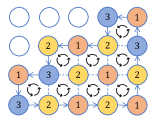
Figure 1: Cancellation of $a$-values.

For each node $u\in V$, we define

$$i(u)=\begin{cases}1&\text{if }c(u)=3,\\ 0&\text{otherwise.}\end{cases}$$

as the indicator variable for $c(u)=3$. We show that the parity of the $b$-value of a directed path is uniquely determined by the colors of the two endpoints and the parity of the path length.

Lemma 3.5 (Parity of $b$-value).

Let $C$ be any directed cycle of length $\ell$ and let $P=(u,\ldots,v)$ be any directed path of length $\ell$. We have

$$b(C)\equiv\ell\pmod{2}\qquad\text{and}\qquad b(P)\equiv i(u)+i(v)+\ell\pmod{2}.$$

backgroundcolor=cyan!25]Mingyang: This offers another proof to show Lemma 3.4, as in the simple grids, all cycles are even.backgroundcolor=blue!25]Yijun: It does not offer a proof for that lemma. It only shows that $b(C)$ is even.

Proof.

We just need to focus on proving $b(P)\equiv i(u)+i(v)+\ell\pmod{2}$, as $b(C)\equiv\ell\pmod{2}$ follows from $b(P)\equiv i(u)+i(v)+\ell\pmod{2}$ by viewing $C$ as a directed path that starts and ends at the same node $u$ and observing that $i(u)+i(u)=0$ regardless of the color of $u$.

Base case.

Suppose $\ell=1$. We claim that $b(P)=a(u,v)\equiv i(u)+i(v)+\ell\pmod{2}$. To see this, we divide the analysis into two cases.

• If $c(u)\neq 3$ and $c(v)\neq 3$, then $a(u,v)\in\{-1,1\}$, so $a(u,v)\equiv i(u)+i(v)+\ell\equiv 1\pmod{2}$, as $i(u)=i(v)=0$.

• If $c(u)=3$ or $c(v)=3$, then $0=a(u,v)\equiv i(u)+i(v)+\ell\equiv 0\pmod{2}$, as $i(u)+i(v)=1$.

Summation.

Now consider the case where $\ell>1$.

$$b(P) =\sum_{(s,t)\in P}a(s,t)$$

$$\equiv\sum_{(s,t)\in P}(i(s)+i(t)+1)\pmod{2}$$ (the base case)

$$\equiv-i(u)-i(v)+2\cdot\sum_{(s,t)\in P}(i(s)+i(t))+\sum_{(s,t)\in P}1\pmod{2}$$

$$\equiv i(u)+i(v)+\ell\pmod{2}$$

Before we continue, we briefly discuss the intuition behind our notion of $b$-value. This notion intuitively captures the level of difficulty in completing the coloring of the rest of the grid given a colored path. In a proper 3-coloring of a grid, the set of nodes with color $3$ separates the remaining nodes into connected regions. In the subsequent discussion, a region refers to a connected set of nodes with colors $1$ and $2$. Let us start by considering a directed path $3\rightarrow 2\rightarrow 1\rightarrow 2\rightarrow 1\rightarrow 2\rightarrow 3$ whose $b$-value is zero. Starting from the coloring of this path, it is easy to extend the partial coloring in a way that the region of nodes colored with 1 and 2 is enclosed by a cycle of nodes colored with 3, see Figure 2.

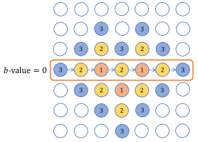
Figure 2: A directed path whose $b$-value is zero.

Now consider a directed path $3\rightarrow 2\rightarrow 1\rightarrow 2\rightarrow 1\rightarrow 3$ whose a $b$-value is 1. In this case, we cannot close the region with one cycle of nodes colored 3. The region of nodes colored with 1 and 2 must continue unless it closes with itself or reaches the boundary of the grid. Consider any directed cycle $C$ that contains the directed path $3\rightarrow 2\rightarrow 1\rightarrow 2\rightarrow 1\rightarrow 3$ as a subpath. Observe that $C$ must intersect with the region of nodes colored with 1 and 2 again via a directed path whose $b$-value is $-1$, as illustrated in Figure 3.

Intuitively, the $b$-value of a directed path counts the difference between the number of occurrences of $3\rightarrow 2\rightarrow\cdots\text{(colors $1$ and $2$ appear alternatively)}\cdots\rightarrow 1\rightarrow 3$ and the number of occurrences of $3\rightarrow 1\rightarrow\cdots\text{(colors $1$ and $2$ appear alternatively)}\cdots\rightarrow 2\rightarrow 3$. The above informal discussion suggests that each occurrence $3\rightarrow 2\rightarrow\cdots\rightarrow 1\rightarrow 3$backgroundcolor=cyan!25]Mingyang: nodes insides paths are colored by $\{1,2\}$ alternativelybackgroundcolor=blue!25]Yijun: Done. has to be matched with an occurrence of $3\rightarrow 1\rightarrow\cdots\rightarrow 2\rightarrow 3$. Therefore, if we can force an algorithm to create a directed path $P$ with a large value of $|b(P)|$, then we may obtain a high locality lower bound for the algorithm.

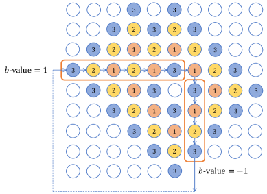
Figure 3: Intersection of a directed cycle and a region of nodes with colors $1$ and $2$.

4 Hardness of 3-Coloring in Simple Grids

In this section, we prove Theorem 1. Our proof uses the following properties of $b$-values in grids.

• The $b$-value of any directed cycle is always zero (Lemma 3.4).

• The parity of the $b$-value of any directed path is solely determined by the parity of the path length and the color of the two endpoints $u$ and $v$ (Lemma 3.5).

To establish Theorem 1, we prove that any algorithm designed for 3-coloring grids, operating with a locality of $T(n)\in o(\log n)$, can be strategically countered by an adversary capable of forcing a directed cycle with a non-zero $b$-value. Throughout this section, let $\mathcal{A}$ be any algorithm for 3-coloring an $\left(\sqrt{n}\times\sqrt{n}\right)$ grid $G=(V,E)$ with a locality of $T(n)\in o(\log n)$. We analyze the coloring function $c\colon V\rightarrow\{1,2,3\}$ generated by algorithm $\mathcal{A}$.

The core strategy of our proof is to create a directed path with a substantial $b$-value, making it impossible for the algorithm to complete the coloring with a small locality. The interaction between the algorithm and the adversary in $\mathsf{Online}$-$\mathsf{LOCAL}$ can be seen as a 2-player game as follows.

• The algorithm’s task is to label each node $v_{i}$ based on the current discovered region $G_{i}$ and the sequence $(v_{1},v_{2},\ldots,v_{i})$. The algorithm wins if the final coloring of $G$ is proper.

• The adversary’s task is to select the nodes $v_{i}$ in the sequence $\sigma=(v_{1},v_{2},\ldots,v_{n})$. Moreover, the adversary has the liberty to adjust how the current discovered region $G_{i}$ fits into $G$ as an induced subgraph. Informally, if $G_{i}$ consists of several connected components, then the adversary has the flexibility to adjust the directions of these components and the distances between these components, as the algorithm is unaware of the precise location of these components in $G$. The adversary wins if the final coloring of $G$ is not proper.

Next, we show that there is an adversary strategy to construct a directed path with a large $b$-value within a row while keeping the discovered region small. Here we only allow our adversary strategy to select nodes within one row, so in the subsequent discussion, we measure the length of the current discovered region $G_{i}$ by the distance between the two farthest nodes in $G_{i}$ restricted to the row, where the distance is measured with respect to the row.

Lemma 4.1.

Let $k$ be a non-negative integer such that $5^{k+1}\cdot T(n)<\sqrt{n}$. There is an adversary strategy to construct a directed path with its $b$-value of at least $k$ within a row while keeping the length of the discovered region at most $5^{k+1}\cdot T(n)$.

Proof.

We prove the lemma by an induction on $k$.

Base case.

For the case where $k=0$, the adversary can just reveal any node $v$. We view node $v$ as a directed path with a $b$-value of zero. The length of the discovered region is $2T(n)<5^{k+1}\cdot T(n)$, as the algorithm has locality $T(n)$.

Inductive step.

Now consider the case where $k\geq 1$. In the subsequent discussion, we write $P_{x,y}$ to denote the directed path starting from $x$ and ending at $y$ along the row. By the induction hypothesis, we construct two directed paths $P_{u,v}$ and $P_{s,t}$ with a $b$-value of at least $k-1$. The construction of both directed paths requires a discovered region of length at most $5^{k}\cdot T(n)$. backgroundcolor=cyan!25]Mingyang: Maybe we could also illustrate another case that node $s$ is on the right of node $t$? Or add explanation that we can force node $s$ always on the left of node $t$backgroundcolor=blue!25]Yijun: For me, I think the current writing is already clear. Before the lemma. there is already some explanation about how we can change directions freely.

We now concatenate these two directed paths together into a directed path $P_{u,t}$ by concatenating the two discovered regions via a path of length $\ell\in\{2,3\}$ on the row.backgroundcolor=cyan!25]Mingyang: Can we choose $l=1$?backgroundcolor=blue!25]Yijun: No, in which case the two regions are no longer disjoint. See Figure 4 for an illustration. After the concatenation, the length of the discovered region is at most $\ell+2\cdot 5^{k}\cdot T(n)\leq 5^{k+1}\cdot T(n)$. Here we use the fact that $T(n)\geq 1$, since obviously $3$-coloring cannot be solved with zero locality.

To finish the proof, we just need to select $\ell\in\{2,3\}$ in such a way that we can find a directed path in the row using the nodes between $u$ and $t$ whose $b$-value is at least $k$. If the $b$-value of one of the paths $P_{u,v}$ and $P_{s,t}$ is already at least $k$, then we are done, so from now on we assume that their $b$-values are precisely $k-1$.

By Lemma 3.5, the parity of the $b$-value of any directed path is solely determined by the parity of the path length and the color of the two endpoints. Therefore, we may select $\ell\in\{2,3\}$ in such a way that the parity of the $b$-value of the path $P_{v,s}$ differs from $k-1$, i.e., $b(P_{v,s})\not\equiv k-1\pmod{2}$.

From now on, we write $h=b(P_{v,s})$, so we have $b(P_{u,t})=2(k-1)+h$. We claim that at least one of $|2(k-1)+h|$ or $|h|$ is greater than $|k-1|$. The claim holds true due to the inequality

$$|2(k-1)+h|+|h|=|2(k-1)+h|+|-h|\geq|2(k-1)|=2\cdot|k-1|$$

and the observation that the inequality becomes equality only when $|h|=|k-1|$, which is impossible because $h\neq k-1$. We conclude that the $b$-value of at least one of the directed paths $P_{v,s}$, $P_{s,v}$, $P_{u,t}$, and $P_{t,u}$ is at least $k$, as required. ∎

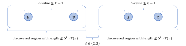
Figure 4: Concatenating $P_{u,v}$ and $P_{s,t}$.

Now we are prepared to prove Theorem 1.

See 1

Proof.

To prove the theorem, we just need to show that any algorithm $\mathcal{A}$ with locality $T(n)\in o(\log n)$ for $3$-coloring a $\left(\sqrt{n}\times\sqrt{n}\right)$ grid is incorrect. As long as $n$ is at least a sufficiently large constant, we may find an integer $k$ to satisfy the two conditions: $k>4T(n)+4$ and $5^{k+1}\cdot T(n)<\sqrt{n}$.

In the subsequent discussion, if $x$ and $y$ are two nodes that belong to the same row or the same column, then we write $P_{x,y}$ to denote the directed path starting from $x$ and ending at $y$ along the row or the column.

In the $\left(\sqrt{n}\times\sqrt{n}\right)$ grid, we apply the adversary strategy of Lemma 4.1 to force the algorithm $\mathcal{A}$ to construct a directed path $P_{u,v}$ in a row $R_{1}$ starting from $u$ and ending at $v$ with $b(P_{u,v})\geq k$. After that, we consider the row $R_{2}$ that is above the row $R_{1}$ by a distance of $2T(n)+2$. Let $t$ be the node in $R_{2}$ that belongs to the same column as $u$. Let $s$ be the node in $R_{2}$ that belongs to the same column as $v$. See Figure 5 for an illustration.

As the adversary, we ask the algorithm to color all the nodes in $P_{s,t}$. We may assume that $b(P_{s,t})\geq 0$. In case $b(P_{s,t})<0$, we can simply reverse the direction of $P_{s,t}$. This is possible because the discovered region associated with $P_{s,t}$ is not connected to the discovered region associated with $P_{u,v}$ from the viewpoint of the algorithm, as the distance between $R_{1}$ and $R_{2}$ is at least $2T(n)+2$.

We let the algorithm finish the coloring of the remaining nodes arbitrarily. Now consider the directed cycle $C$ formed by concatenating the four directed paths $P_{u,v}$, $P_{v,s}$, $P_{s,t}$, and $P_{t,u}$. By its definition, the absolute value of the $b$-value of one path $P$ is at most its length, so the $b$-value of both $P_{v,s}$ and $P_{t,u}$ is at least $-(2T(n)+2)$, so

$$b(C)=b(P_{u,v})+b(P_{v,s})+b(P_{s,t})+b(P_{t,u})\geq k-(2T(n)+2)+0-(2T(n)+2)>0,$$

which is impossible due to Lemma 3.4, so the coloring produced by the algorithm is incorrect. ∎

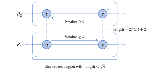
Figure 5: Construction of a directed cycle with non-zero $b$-value

5 Hardness of 3-Coloring in Toroidal and Cylindrical Grids

In this section, we prove Theorem 2.

See 2

Proof.

We start by discussing the properties of proper 3-coloring of toroidal and cylindrical grids. Consider any two directed cycles $C_{1}$ and $C_{2}$ corresponding to orienting two rows with different directions. Same as the proof of Lemma 3.4, we may calculate $b(C_{1})+b(C_{2})$ alternatively by summing up the $b$-value for the cells located between $C_{1}$ and $C_{2}$, so we infer that

$$b(C_{1})+b(C_{2})=0.$$ (1)

Furthermore, if the number of columns is odd, then the lengths of the two directed cycles $C_{1}$ and $C_{2}$ are odd, so Lemma 3.5 implies that both $b(C_{1})$ and $b(C_{2})$ are odd numbers.

Consider an arbitrary algorithm $\mathcal{A}$ designed for 3-coloring $\left(\sqrt{n}\times\sqrt{n}\right)$ cylindrical or toroidal grids with locality $T(n)\in o(n^{1/2})$. Let us choose a sufficiently large value of $n$ such that $\sqrt{n}$ is an odd number and $4T(n)+4\leq\sqrt{n}$. Therefore, we may select two rows such that their $T(n)$-radius neighborhoods induce non-adjacent cylindrical grids with $2T(n)+1$ rows and $\sqrt{n}$ columns.

As the adversary, we instruct algorithm $\mathcal{A}$ to color these two rows. From the perspective of the algorithm, it sees precisely two disjoint cylindrical grids with $2T(n)+1$ rows and $\sqrt{n}$ columns. Furthermore, the algorithm is unaware of their positions and directions in the input graph. As the adversary, we have the liberty to choose their directions after the algorithm fixes the coloring of the two rows. Since the $b$-value of an odd-length directed cycle is odd, we can always select their directions to violate Equation 1. Hence the algorithm $\mathcal{A}$ cannot correctly 3-color the graph. ∎

We remark that the $\Omega(\sqrt{n})$ locality lower bound in the proof above comes from the fact that the number of rows is $\sqrt{n}$. If we consider a general $(a\times b)$ toroidal or cylindrical grid, then the above proof yields an $\Omega(a)$ locality lower bound whenever the number of columns $b$ is an odd number.

References

- [AEL+23] Amirreza Akbari et al. “Locality in Online, Dynamic, Sequential, and Distributed Graph Algorithms” In 50th International Colloquium on Automata, Languages, and Programming (ICALP 2023) 261, Leibniz International Proceedings in Informatics (LIPIcs) Dagstuhl, Germany: Schloss Dagstuhl – Leibniz-Zentrum für Informatik, 2023, pp. 10:1–10:20 DOI: 10.4230/LIPIcs.ICALP.2023.10
- [AOS+18] Sepehr Assadi, Krzysztof Onak, Baruch Schieber and Shay Solomon “Fully dynamic maximal independent set with sublinear update time” In Proceedings of the 50th Annual ACM SIGACT Symposium on Theory of Computing (STOC), 2018, pp. 815–826
- [BCH+18] Sayan Bhattacharya, Deeparnab Chakrabarty, Monika Henzinger and Danupon Nanongkai “Dynamic algorithms for graph coloring” In Proceedings of the Twenty-Ninth Annual ACM-SIAM Symposium on Discrete Algorithms (SODA), 2018, pp. 1–20 SIAM
- [BHK+17] Sebastian Brandt et al. “LCL problems on grids” In Proceedings of the ACM Symposium on Principles of Distributed Computing (PODC), 2017, pp. 101–110
- [BM19] Leonid Barenboim and Tzalik Maimon “Fully dynamic graph algorithms inspired by distributed computing: Deterministic maximal matching and edge coloring in sublinear update-time” In Journal of Experimental Algorithmics (JEA) 24 ACM New York, NY, USA, 2019, pp. 1–24
- [CKP19] Yi-Jun Chang, Tsvi Kopelowitz and Seth Pettie “An Exponential Separation between Randomized and Deterministic Complexity in the LOCAL Model” In SIAM Journal on Computing 48.1, 2019, pp. 122–143
- [CP19] Yi-Jun Chang and Seth Pettie “A Time Hierarchy Theorem for the LOCAL Model” In SIAM Journal on Computing 48.1, 2019, pp. 33–69
- [DKK13] Stefan Dobrev, Rastislav Královič and Richard Královič “Independent set with advice: the impact of graph knowledge” In Approximation and Online Algorithms: 10th International Workshop (WAOA 2012), 2013, pp. 2–15 Springer
- [GK18] Manoj Gupta and Shahbaz Khan “Simple dynamic algorithms for maximal independent set and other problems” In arXiv preprint arXiv:1804.01823, 2018
- [GKM17] Mohsen Ghaffari, Fabian Kuhn and Yannic Maus “On the complexity of local distributed graph problems” In Proceedings of the 49th Annual ACM SIGACT Symposium on Theory of Computing (STOC), 2017, pp. 784–797
- [IL93] Zoran Ivković and Errol L Lloyd “Fully dynamic maintenance of vertex cover” In International Workshop on Graph-Theoretic Concepts in Computer Science (WG), 1993, pp. 99–111 Springer
- [Lin92] Nathan Linial “Locality in distributed graph algorithms” In SIAM Journal on computing 21.1 SIAM, 1992, pp. 193–201
- [NS15] Ofer Neiman and Shay Solomon “Simple deterministic algorithms for fully dynamic maximal matching” In ACM Transactions on Algorithms (TALG) 12.1 ACM New York, NY, USA, 2015, pp. 1–15
- [Pel00] David Peleg “Distributed computing: a locality-sensitive approach” SIAM, 2000
- [RG20] Václav Rozhoň and Mohsen Ghaffari “Polylogarithmic-Time Deterministic Network Decomposition and Distributed Derandomization” In Proceedings of the 52nd Annual ACM SIGACT Symposium on Theory of Computing (STOC), 2020, pp. 350–363