Brain Decodes Deep Nets

Abstract

We developed a tool for visualizing and analyzing large pre-trained vision models by mapping them onto the brain, thus exposing their hidden inside. Our innovation arises from a surprising usage of brain encoding: predicting brain fMRI measurements in response to images. We report two findings. First, explicit mapping between the brain and deep-network features across dimensions of space, layers, scales, and channels is crucial. This mapping method, FactorTopy, is plug-and-play for any deep-network; with it, one can paint a picture of the network onto the brain (literally!). Second, our visualization shows how different training methods matter: they lead to remarkable differences in hierarchical organization and scaling behavior, growing with more data or network capacity. It also provides insight into finetuning: how pre-trained models change when adapting to small datasets. Our method is practical: only 3K images are enough to learn a network-to-brain mapping.

1 Introduction

The brain is massive, and its enormous size hides within it a mystery: how it efficiently organizes many specialized modules with distributed representation and control. One clue it offers is its hierarchical organization. This hierarchical structure facilitates efficient computation, continuous learning, and adaptation to dynamic tasks.

Deep networks are massive, containing billions of parameters. Performances keep improving with more training data and larger size. It doesn’t seem to matter if the network is trained under the supervision of labels, weakly supervised with image captions, or even self-supervised without human-provided guidance [60]. Its massiveness also hides within a mystery: as its size increases, it can be fine-tuned successfully to many unseen tasks.

What can these two massive systems, the brain and deep network, tell about each other? The emergence of large-scale, high-quality, open-source brain fMRI recordings has led to state-of-the-art brain encoding models [9, 19].

The key insight is that even if two deep network features can produce a similar brain encoding, their underlying computation could be drastically different. By identifying ‘what’ deep features in space, layer, and scale are most relevant for each brain voxel fMRI prediction, we can obtain a picture of deep features mapped onto a brain (literally), as shown by the brain-to-network mapping in Figure 1.

Our analysis crucially depends on a robust mapping between deep 4D features: spatial, layer, channel, and scale (class token vs local token) to the brain. Our fundamental assumption is that this mapping should be: a) brain-topology constrained, and b) factorized in feature dimensions of space, layer, channel, and scale. This is important because independent 4D image features to brain mapping are highly unconstrained, and learning a shared mapping across images, with brain-topology constraint and factorized representation, is statistically more stable.

The picture of brain-to-network mapping tells us about the deep network from the brain’s perspective. For example, how does the hierarchical organization of deep networks correspond to the hierarchical organization of the brain? Suppose the brain’s hierarchical organization is a template for efficient, modular, and generalizable computation; an ideal computer vision model should align with the brain: the first layer of the deep network matches the early visual cortex, and the last layer best matches high-level regions. Surprisingly, the CLIP network is more aligned with the brain than newer and more powerful self-trained networks, and its hierarchy organization increases when we increase the model’s capacity, while self-supervised methods become less hierarchically organized. Furthermore, networks with more hierarchy organization tend to maintain their hidden layers better when finetuning on small datasets. We conjuncture that better alignment to the brain is one way to find a robust model that adapts to dynamic tasks.

Our method is practical; instead of using typically 22K images to learn, it needs only 3K images (30 minutes) to learn for the network visualization. In summary:

1. We introduce a factorized, brain-topological smooth selection that produces an explicit mapping between deep features: space, layer, channel, and scale (class token vs local token) to the brain.

2. We pioneer a new network visualization by coloring the brain using layer-selectors, exposing the inner workings of the network.

2 Related Work

Benchmarks and Competitions

Open challenges on brain encoding have generated broad interests [19, 9, 10, 51, 52, 62, 59]. Large-scale datasets are growing rapidly in both quantity and quality [31, 7, 2, 24, 18]. The Algonauts 2023 challenge [19] is the first to use a massive high-quality 7-Tesla fMRI dataset [2]. The high quality of the datasets enabled models that can recover retinotopy from naturalistic image stimuli [47], which was only possible in synthetic stimuli experiments [15].

Explain Brain by Deep Networks

Gradient-based methods have been used to explain how brain works: orientation-selective neurons in V1 [47, 16, 37], category-selective regions in late visual brain [45, 28, 50, 34, 42, 35]. Gradient-based methods can also generate maximum-excited images [4, 20, 30, 55]. Meanwhile, studies try to find the best performance pre-trained model for each brain ROI [12, 70, 40, 49, 61] from a zoo of supervised [44, 54, 29, 27], self-supervised [23, 8, 41, 21, 32], image generation [46], and 3D [38, 48, 58] models. Features can be efficiently cached and are plug-in-and-play [60, 22, 57]. Our work goes in the opposite direction: use the brain to explain deep networks.

Brain-to-Network Alignments

Starting from V1, neurons in the visual cortex were found to have increasing receptive field size and represent more abstract concepts [15, 14, 65]. Existing works found deep network layers hierarchically align with visual stream [51, 52, 31, 9, 66, 60]. However, existing work only explained brain-to-network mapping at ROI-level. Voxel-level mapping was challenging due to the underconstrained nature of the brain data. This work introduces topological smooth constraints and successfully extends to the voxel-level.

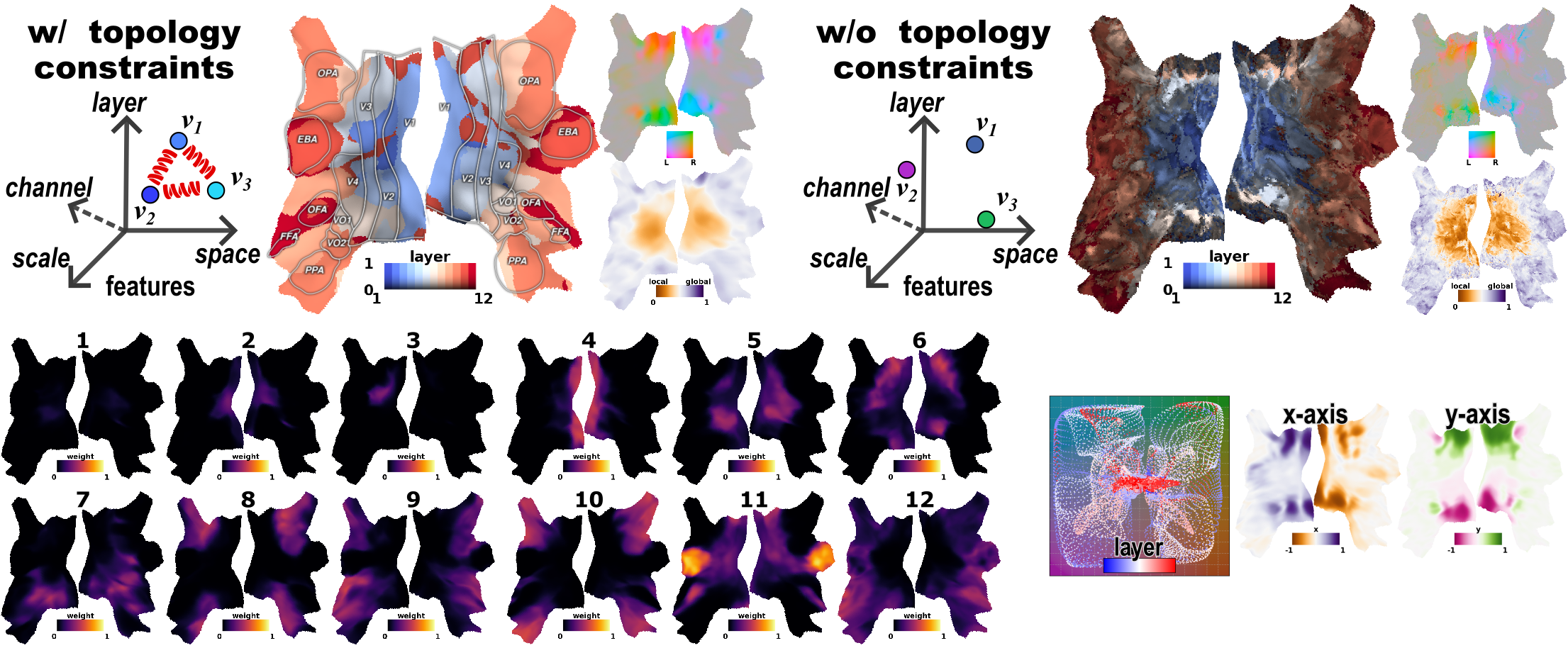
Figure 2: Topological Constrained, Factorized, Brain-to-Network Selectors for CLIP. Top: factorized-selectors trained with topological constraints improved confidence of the mapping (color brightness) and mapping smoothness (colored as Section 3.2). Bottom left: individual layer-selector weight $\bm{\hat{\omega}}^{layer}$, note layer 4 is mostly aligned with V1, and the last two are aligned with the body (EBA) and face (FFA) region. Bottom right: space-selector $\bm{\hat{u}}^{space}$: 3D voxels, dots, are mapped to the image space with color dots indicating the layers. For later layers, only center image regions are selected.

3 Methods: Brain Encoding Model

Figure 1 presents an overview of our methods. In the brain encoding task, one needs to predict a large number voxels (vertices), of visual cortex’s fMRI responses as a function of the observed image. This encoding task is underconstrained: since each subject has her/his unique mental process, a successful brain encoding model needs to be highly individualized, thus significantly reducing the training example per voxel. Most of the current approaches treat each brain voxel independently. This leads to a major reduction in signal-to-noise ratio, particularly for our analysis.

Our fundamental innovations are two-fold. First, we enforce brain-and-network topology-constrained prediction. Brain voxels are not independent but are organized locally into similar “tasks”, and globally into diverse functional regions. Similarly, Neural networks show local feature similarity across adjacent layers while ensuring diversity for far-away ones. The local smoothness constraints significantly reduce uncertainties in network-to-brain mapping.

Second, we propose a factorized feature selection across three independent dimensions of space, layers, and scales (local vs global token). This factorized representation leads to a more robust estimation because feature selection in each dimension is more straightforward, and learning can be more efficient across training samples. For example, the spatial feature selection only needs to find the center of the pixel region for each brain voxel, similar to retinotopy. The layer or scale selection estimates the size of the pixel region: the early layer typically has a smaller receptive field size. Note that the factorized feature selection is soft: multiple layers or spatial locations can be selected, as determined by the brain prediction training target.

3.1 Factorized, Topological Smooth, Brain-to-network Selection (FactorTopy)

We used a pre-trained image backbone model (ViT) to process input image $\bm{X}$ into features $\bm{V}$. The entire feature $\bm{V}$ is organized along four dimensions: space, layer, scale (class token and local tokens), and channels. The brain encoding prediction target $\bm{Y}\in\mathbb{R}^{N\times 1}$ is beta weights of hemodynamic response function [43]. Denote $y_{i}$ the individual voxel $i\in\{1,2,\dots,N\}$ response.

The current state-of-the-art methods [2, 50] compute a layer-specific, scale-specific, 2D spatial feature selection mask to pool features $\bm{V}\in\mathbb{R}^{L\times C\times H\times W}$ along spatial dimension $H\times W$ into a vector of $\mathbb{R}^{L\times C}$, where $L$ denotes layer and $C$ is channel. Instead, we propose a factorized feature selection method where, for each voxel, we select the corresponding space, layer, and scale in each dimension.

Essentially, a voxel asks: ‘What is the best x-factor for my brain prediction?’ where the x-factor is one of the layer, space, scale, or channel dimensions.

1) space selector. $selSpace:\enspace\mathbb{R}^{N\times 3}\rightarrow\bm{\hat{u}}^{space}\in\mathbb{R}^{N\times 2}$, maps a brain voxel into a 2D image coordinate. We used linear interpolation Interp to extract $\bm{\bar{\nu}}_{i,l}^{local}\in\mathbb{R}^{1\times C}$.

2) layer selector. $selLayer:\enspace\mathbb{R}^{N\times 3}\rightarrow\bm{\hat{\omega}}^{layer}\in\mathbb{R}^{N\times L}$, produces $\hat{\omega}_{i,l}^{layer}\in[0,1]$ weight for each layer $l$, such that $\sum_{l=1}^{L}\hat{\omega}_{i,l}^{layer}=1$. We take a weighted channel-wise average of feature vectors $\bm{\bar{\nu}}_{i,l}$ across all layers.

3) scale selector: $selScale:\enspace\mathbb{R}^{N\times 3}\rightarrow\bm{\hat{\alpha}}^{scale}\in\mathbb{R}^{N\times 1}$, computes a scalar $\hat{\alpha}_{i}^{scale}\in[0,1]$ as the weight for local $\bm{\bar{\nu}}_{i,l}^{local}$ vs global token $\bm{\bar{\nu}}_{*,l}^{global}$. Note that $\bm{\bar{\nu}}^{local}_{i,l}$ is unique for each voxel, $\bm{\bar{\nu}}_{*,l}^{global}$ is same for all voxels.

Taking weighted averages over channels across layers could be problematic because channels in each layer represent different information. We need to preemptively align the channels into a shared $D$ dimension channel space. Let $B_{l}$ be a layer-unique channel transformation:

channel align. $B_{l}(\bm{V}_{l}):\enspace\mathbb{R}^{C\times M}\rightarrow\mathbb{R}^{D\times M}$, where $M=(H\times W+1)$.

To obtain the final brain prediction $y_{i}$, we apply feature selection across the channels:

4) channel selector. $\bm{w}_{i}:\enspace\mathbb{R}^{D}\rightarrow\mathbb{R}^{1}$, where $\bm{w}_{i}$ answers, ‘Which is the best channel for predicting this brain voxel?’ Putting it all together, we have

$$\bm{V} =\texttt{ViT}(\bm{X})$$

$$\bm{\bar{\nu}}^{local}_{i,l} =\texttt{Interp}(\bm{\hat{u}}_{i}^{space};B_{l}(\bm{V}_{l}))\quad\quad\quad\quad\quad\quad\quad\quad\text{(1)}$$

$$\bm{v}_{i} =\sum_{l=1}^{L}\hat{\omega}_{i,l}^{layer}((1-{\hat{\alpha}_{i}}^{scale})\bm{\bar{\nu}}^{local}_{i,l}+{\hat{\alpha}_{i}}^{scale}\bm{\bar{\nu}}_{*,l}^{global})$$

$$y_{i} =\bm{v}_{i}\bm{w}_{i}+b_{i}$$

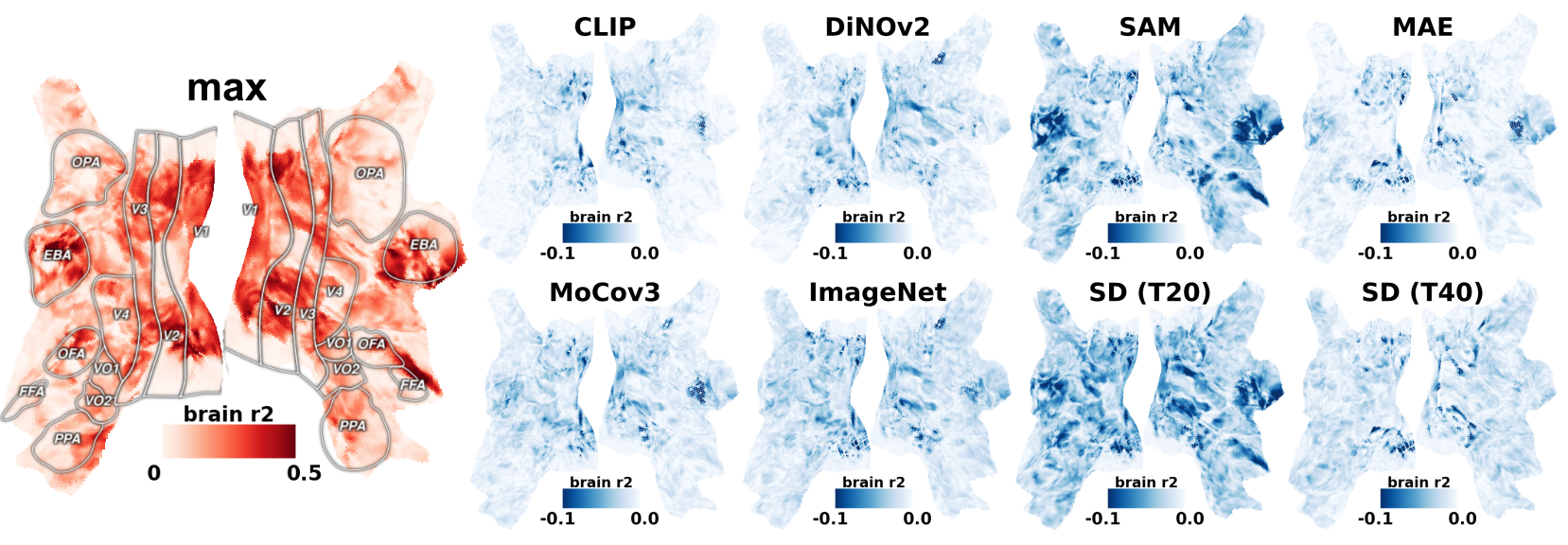
Figure 3: Brain Score. Left: raw brain score $R^{2}$. Right: difference of score to the model-wise max score (left). Insights: 1) CLIP and DiNOv2 predict semantic regions better but relatively weak for early visual, 2) SAM and MAE are better at early visual region but weaker for body (EBA) and face (FFA) region, 3) Stable Diffusion (SD) shows a good prediction in all regions overall.

Topological Smooth.

The factorized selector explicitly maps the brain and the network. The topological structure of the corresponding brain voxels should also constrain this mapping. The smoothness constraint can be formulated as Lipschitz continuity [3]: nearby brain voxels should have similar space, layer, and scale selection values. We apply sinusoidal position encoding [38] to brain voxel.

3.2 Visualization and Coloring

To visualize layer-to-brain mapping, we assign each voxel a color cue value associated with the layer with the highest layer selection value: $\texttt{argmax}_{L}(\bm{\hat{\omega}}^{layer})\in\mathbb{R}^{N\times 1}$. We assign voxel color brightness with a confidence measure $\bm{s}\in\mathbb{R}^{N\times 1}$ of $\bm{\hat{\omega}}^{layer}$:

$$\hskip 42.67912pts_{i}=1-\frac{{\sum_{l=1}^{L}\hat{\omega}_{i,l}^{layer}\log\hat{\omega}_{i,l}^{layer}}}{{\sum_{l=1}^{L}\frac{1}{L}\log\frac{1}{L}}}\hskip 42.67912pt\text{(2)}\hfilneg$$

Note that $s_{i}$ equals 1 when $\bm{\hat{\omega}}_{i}^{layer}$ is a one-hot vector, and 0 when it is uniform. In Figure 2, we compare layer-selector trained with vs. without topological smooth constraints using this layer-to-brain color scheme. Topological smoothness significantly improved selection certainty.

4 Results

For a fair comparison, we keep the same ViT network architecture while varying how the network is trained and the dataset used (Table 2). In Fig. 4, we display network layer-to-brain mapping for several popular pre-trained models. An overview of our experiments:

1. What can relative brain prediction scores tell us?

2. How do supervised and un-supervised training objectives change brain-network alignment?

3. Do more data and larger model sizes lead to a more evident hierarchical structure?

4. What happens to a pre-trained network when finetuning to a new task with small samples?

5. Can the network channels be grouped to match well with brain functional units?

Dataset

We used Nature Scenes Dataset (NSD) for this study [2]. Briefly, NSD provides 7T fMRI scan when watching COCO images [33]. A total of 8 subjects each viewed 3 repetitions of 10,000 images. We used the preprocessed and denoised single-trail data of the first 3 subjects [43]. We split 27,750 public trials into train validation and test sets (8:1:1) and ensured no data-leak of repeated trials.

4.1 Brain Score for Downstream Tasks Prediction

The key finding is that a network with a high prediction score on a specific brain region is better suited for a relevant downstream task. CLIP, DiNOv2 and Stable Diffusion have overall high performance.

Let $R^{2}=1-\sum(y_{i,m}-\hat{y}_{i,m})^{2}/\sum(y_{i,m}-\bar{y}_{i,m})^{2}$ be the brain score metrics, $R^{2}$ is computed for each voxel $i$ over the test-set $m$. We report the raw score without dividing by noise ceiling or averaging repeated trials [19]. We compared the brain score for each model to the ‘max’ model constructed by model-wise maximum for each voxel. We show the raw $R^{2}$ in Figure 3, and ROI-wise root sum squared difference to the ‘max’ in Table 1.

Model	Dataset	Root Sum Squared Difference $R^{2}$ $\downarrow$
		V1	V2V3	OPA	EBA	FFA	PPA
Known Selectivity		orientation		navigate	body	face	scene
max		0.237	0.215	0.097	0.185	0.186	0.134
CLIP [44]	DC-1B [17]	0.032	0.023	0.011	0.015	0.005	0.006
DiNOv2 [41]	LVD-142M	0.033	0.026	0.021	0.013	0.008	0.007
SAM [29]	SA-1B	0.037	0.033	0.025	0.065	0.056	0.033
MAE [23]	IN-1K	0.031	0.025	0.008	0.029	0.017	0.009
MoCov3 [8]	IN-1K	0.032	0.027	0.014	0.031	0.015	0.011
ImageNet [13]	IN-1K	0.037	0.032	0.024	0.028	0.019	0.015
SD (T20) [46]	LAION-5B [53]	0.047	0.050	0.029	0.056	0.052	0.032
SD (T40) [46]	LAION-5B	0.031	0.030	0.021	0.018	0.019	0.013

Table 1: Brain Score. Raw $R^{2}$ for max of all models and root sum squared difference for other models.

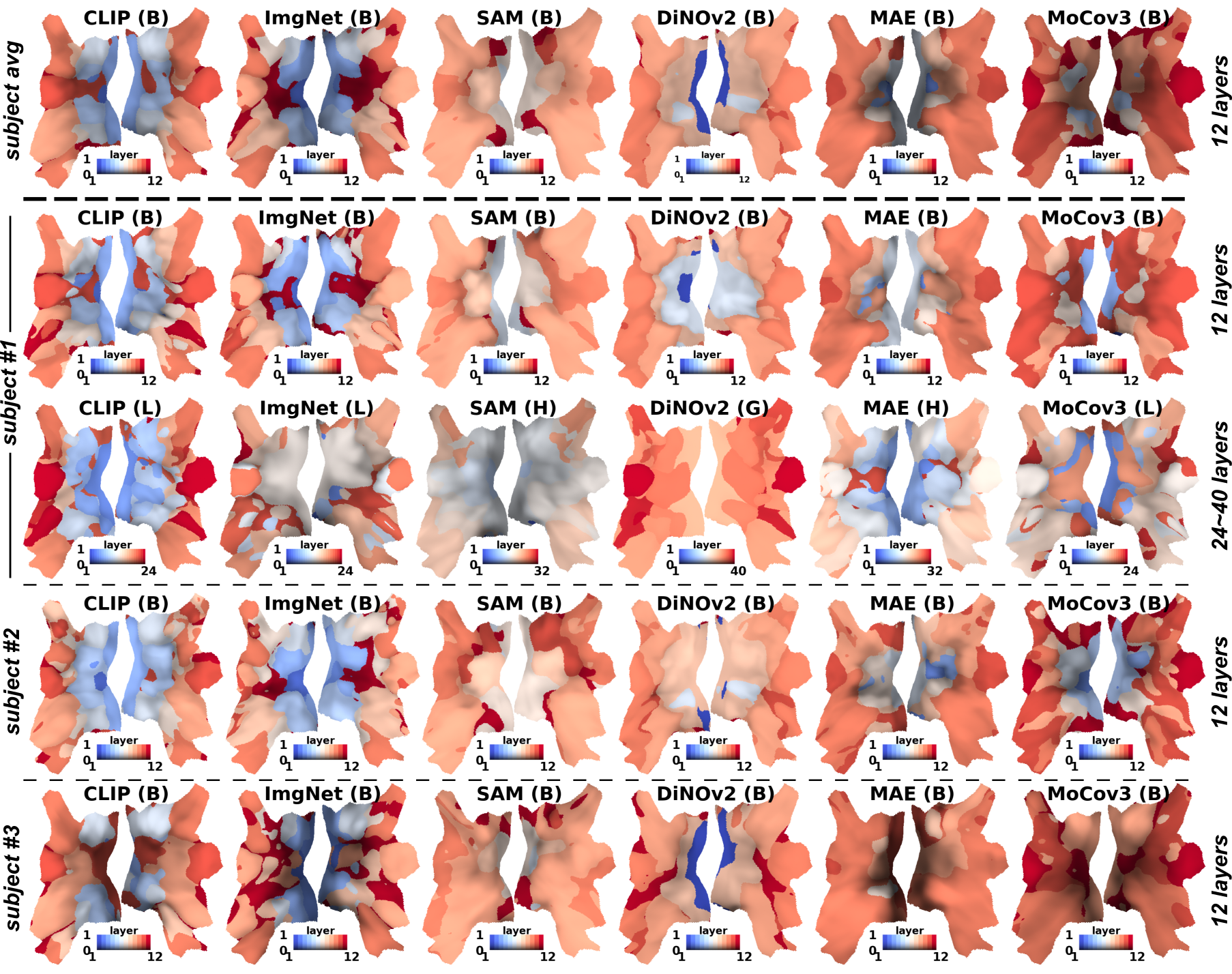
Figure 4: Layer Selectors, Brain-Network Alignment. All models are ViT architecture, number of layers is marked in the colorbar x-axis. Brightness is confidence measurement (defined in Section 3.2), and lower brightness means a softer selection of multiple layers. Top: average of three subjects, base size 12-layer model. Middle: subject #1, 12 layer small(S) and base(B) model, 24 layer large(L) model, 32 layer huge(H) model, 40 layer gigantic(G) model. Bottom: subject #2 and #3, base size 12-layer model. Insights: 1) CLIP layers align best with the brain’s hierarchical organization, 2) ImageNet and SAM last layer align with mid-level in the brain, indicating their training objectives aimed at mid-level concept; 3) DiNOv2: with a larger model, its hierarchy no longer align with the brain.

Model	CLIP [26]				ImageNet [13]		SAM [29]			DiNOv2 [41]			MAE [23]			MoCov3 [8]
Size	L/14	B/16	B/32	B/32	L	B	H	L	B	G	L	B	H	L	B	L	B	S
Data	1B [17]	140M	14M	1.4M	IN-1K [13]		SA-1B [29]			LVD-142M [41]			IN-1K [13]			IN-1K [13]
$R^{2}$ $\uparrow$	0.132	0.131	0.117	0.083	0.117	0.121	0.120	0.117	0.111	0.123	0.125	0.128	0.132	0.129	0.128	0.124	0.127	0.126
slope $\uparrow$	0.53	0.50	0.32	0.11	0.27	0.39	0.08	0.10	0.15	0.16	0.25	0.41	0.20	0.37	0.32	0.30	0.33	0.40
$b_{0}$ $\downarrow$	0.35	0.38	0.49	0.60	0.41	0.45	0.58	0.63	0.67	0.76	0.66	0.50	0.46	0.47	0.55	0.40	0.52	0.51
$b_{1}$ $\uparrow$	0.88	0.88	0.82	0.71	0.68	0.83	0.66	0.73	0.82	0.92	0.92	0.91	0.66	0.84	0.87	0.70	0.85	0.91

Table 2: Layer Selectors, Brain-Network Alignment. Brain-network alignment is measured by slope and intersection of linear fit (defined in Section 4.3). Larger slope means generally better alignment with the brain, smaller $b_{0}$ means better alignment of early layers, and larger $b_{1}$ means better alignment of late layers. $R^{2}$ is brain score. Bold marks the best within the same model. Insights: 1) CLIP’s alignment to the brain improves with larger model capacity, 2) for all others, bigger models decrease the brain-network hierarchy alignment.

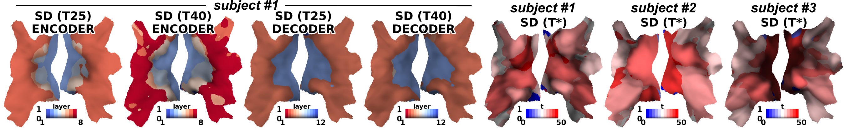
Figure 5: Diffusion Models. Left: one time step (T=25 and T=40) layer selection, UNet encoder and decoder layers. Right: fix layer (UNet decoder layer 6) time step selection. Color brightness is confidence measure (Section 3.2). Insights: 1) Diffusion models have less delineation in brain-network mapping using fixed time-step encoder/decoder layers, but more separation when using time steps, 2) mid-late time steps align with higher level brain, late time step aligns with early brain region.

Figure 3 shows that the fovea regions of early visual cortex are highly predictable, and so are higher regions of EBA and FFA, followed by PPA. In Table 1, we found DiNOv2 and CLIP predict well on EBA and FFA but poorly for early visual regions; MAE and SAM are the opposite. Stable Diffusion (SD) features, described in the next section, perform well in all regions. This finding is consistent with recent works that show SD features are helpful for many visual tasks, from segmentation to semantic correspondence [64, 56]. It could also explain why a combination of DiNOv2 for coarser semantic correspondence with SD for finer alignment could work well [68, 60].

4.2 Training Objectives and Brain-Net Alignment

The key finding is training objective matters: 1) supervised methods show a more detailed delineation of network-to-brain mapping compared to self-supervised ones; 2) ImageNet and SAM show the last layer mapped to the middle region of the brain; 3) Stable Diffusion features show more detailed delineation between the time steps than between the UNet encoder or decoder layers.

The layer multi-selector output indicates, “within one model, which layer best predicts this brain region?”. Even though the mapping differs for subjects (Figure 4), the pattern of subject difference is consistent in both CLIP and ImageNet models: subject #3 had considerably low confidence in early visual brain, and subjects #2 and #3 are missing the FFA (face) region that subject #1 has.

For supervised pre-trained models, Figure 4 shows CLIP’s [44] last layer is close to EBA for subject average and EBA/FFA for subject #1, probably because the training data contain languages related to body and face. Surprisingly, ImageNet’s [13] last layer is close to the mid-level lateral stream, suggesting that simple image labels are more primitive than text language. SAM’s [29] final layer is close to the mid-level ventral and parietal stream, indicating segmentation as a mid-level visual task. These observations suggest a bottom-up feature computation and top-down task prediction in ImageNet and SAM.

For the self-supervised models, the final layer of DiNOv2 (DiNOv1+iBOT) [41, 69, 6] and MAE [23] is missing from the network-to-brain mapping, which indicates the last stage of un-supervised mask reconstruction deviates from the brain tasks. For MoCov3 [8], there’s a trend that the second-last layer matched more with the ventral stream (“what” part of the brain) than the parietal stream (“where” part), indicating self-contrastive learning is more focused on the semantics rather than spatial relationship [60].

We also analyzed Stable Diffusion [46] by 1) fixing the time step and selecting layers, and 2) fixing the UNet decoder layer 6 and selecting time steps. We followed the “inversion” [36] time steps feature extraction and used a total of T$=$50 time steps. In Figure 5, layer selection showed that the diffusion model has less separation for early and late regions; this was true for both T$=$25, T$=$40, encoders and decoders. Time step selection showed diffusion model early time steps (T$<$25) deviate from the brain tasks. The confidence (Section 3.2) of time step selection was relatively high for EBA at (T$=$30) and for mid-level visual stream at (T$=$35, T$=$40). Overall, our results indicate that 1) the diffusion model has less feature separation across layers but instead is separated across time steps, and 2) global features are more in the middle-time steps, while local features are more aligned with the mid-to-late time steps.

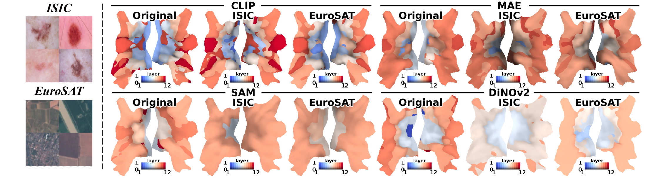
Figure 6: Finetuned to Small Datasets. Left: example images from ISIC and EuroSAT. Right: layer selector (Colored as Section 3.2) before and after finetuning. The whole network is finetuned. Insights: CLIP finetunes with less change in the existing computation.

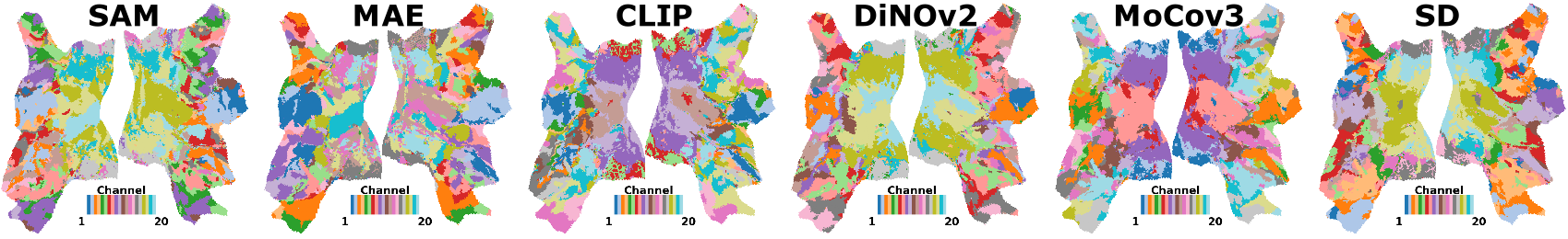
Figure 7: Channel Clustering. Brain voxels clustered by channel selection weight $\bm{w}_{i}$. Insights: early visual brain uses less diverse channels but more diverse spatial locations (Figure 2), higher level brain is the opposite.

4.3 Network Hierarchy and Model Sizes

The key findings are: 1) CLIP shows a more substantial alignment of hierarchical organization with the brain; 2) when scaling with more data and bigger model size, CLIP shows an improvement in its brain-hierarchical alignment, while others show a decrease.

We propose a measure called hierarchy slope by putting predefined brain ROI regions into a number-ordering and fitting a linear regression as a function of their layer selector output $\bm{\hat{\omega}}^{layer}$. We used only coarse brain regions and did not consider feedback computation in the brain.

Hierarchy slope Let $\hat{\iota}_{i}=\sum_{l=1}^{L}\frac{l-1}{L-1}\hat{\omega}_{i,l}^{layer}$ be a scalar that represents vector layer selector weights $\bm{\hat{\omega}}_{i}^{layer}$, such that $\hat{\iota}_{i}\in[0,1]$. We pre-defined a four-level brain structure: 1) V1, 2) V2&V3, 3) OPA, 4) EBA. Voxels inside these ROIs are assigned with an ideal value $\iota_{i}\in\{0,0.33,0.66,1\}$. We fit a linear regression $\hat{\iota}_{i}=\beta\iota_{i}+\epsilon$, where slope $\beta$ measures brain-model alignment, $b_{0}=\epsilon$ and $b_{1}=\beta+\epsilon$ measures the proportion of early and late layer not being selected.

We found that both qualitatively (Figure 4) and quantitatively (Table 2), layer-to-brain alignment is best in the CLIP model. Furthermore, the hierarchy alignment increases as CLIP scaled up both model size and data (slope 0.32 for M, 0.50 for L, 0.52 for XL). CLIP M and S models were trained with the same model size but smaller data; the S model dropped slope significantly (0.11). ImageNet, SAM, MAE, and MoCov3 models show decreased hierarchy slope when scaling up [60]; their late layers were less selected for bigger models, indicating a decreasing hierarchical alignment with the brain. For DiNOv2, the slope (hierarchical alignment) also decreased with a larger model.

4.4 Fine-tuned Model

The key findings are: 1) CLIP maintains a hierarchical structure and uses less re-wiring for downstream tasks; 2) DiNOv2 and SAM tend to re-wire their intermediate layers and lose their hierarchical structure rapidly when finetuned.

We finetuned on two small-scale downstream tasks, ISIC [11] skin cancer classification, and EuroSAT [25] satellite land-use classification. We used 50 training samples per class to train. The pre-trained model is finetuned across all layers with AdamW optimizer lr=3e-5, weight decay of 0.01, batch size of 4, for 3,000 steps. We verified that the finetuned models reached maximum validation performance without significant overfitting.

We apply brain-to-network mapping to visualize the finetuned networks. The first dataset ISIC skin cancer classification relies on low-level features. Figure 6 shows ImageNet/CLIP’s last layer aligned with V1 after ISIC finetuning, potentially indicating the usage of top-down information for low-level vision tasks. The second dataset, EuroSAT, requires less finetuning on low-level features; V1 is still aligned to early layers for CLIP. After finetuning on both datasets, CLIP maintained a strong hierarchical alignment, while SAM and DiNOv2 largely lost their hierarchy. Overall, CLIP adapts to dynamic tasks with less re-wiring of existing computation layouts.

4.5 Channels and Brain ROIs

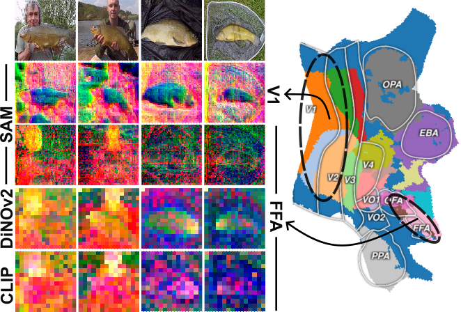
Figure 8: Visualization of top channels in brain ROIs. V1 shows edge selectivity, and FFA shows face selectivity.

The key findings are: 1) we can cluster brain voxels using the co-occurrence of brain voxels with channels, and the clusters largely align well with known brain ROIs; 2) we can compute brain ROI/cluster-specific responses on images to reveal the ROI functionality.

Recall our factorized multi-selector method compresses information across 4D network features into a channel-wise vector of $\bm{v}_{i}$ for each brain voxel $i$. Furthermore, channels across all the layers are aligned (Methods 3.1), resulting in a layer-agnostic channel representation. From that, a linear regression weight vector $\bm{w}_{i}$ acts as a channel selector to determine “which feature channels best predict this brain voxel?” We can view this channel feature selector, $\bm{w(k)}_{i}$, as co-occurrence between brain voxel $i$ and channel elements $k$, which can be used to cluster the brain voxels: linking two voxels, $i,j$ if they share similar channel selectors $\bm{w}_{i}$, $\bm{w}_{j}$. Figure 7 shows the result of clustering brain voxels into 20 clusters.

The higher-level brain utilized diverse channels across the brain areas; there is a consistent pattern that the face and body region use the same channel in CLIP, DiNOv2, MoCov3, and SD. The early visual brain used similar channels across the visual cortex; there is a consistent pattern that the left and right brain are symmetrical, as well as the ventral and parietal streams. SAM and MAE early visual brain-selected channels are non-symmetrical, indicating shift variant properties [60].

The selected channels reveal brain ROI’s functionality. We visualized the top components of selected channels for each ROI in Figure 8, which shows the brain ROIs encode edge information in V1 and face in FFA. Interestingly, DiNOv2 generalizes face across humans and fish [60, 68].

5 Ablation Study

5.1 Performance and Complexity

Previous state-of-the-art brain encoding approaches made diverse choices on image encoders and feature selections. We re-implemented them to avoid unfair comparison by keeping their most salient design choices but swapping them in standard components. We used CLIP-XL [26, 17] backbone for the image encoder for all methods.

There are three distinct types of feature selections. 1) The simplest way is to leverage the class tokens, classToken, by taking it from each layer, $\mathbb{R}^{L\times C}$, applies a layer-unique transformation to $\mathbb{R}^{L\times D}$, and average pools across the layers to obtain a $\mathbb{R}^{D}$ feature vector. 2) The second way, patchComp, extracts information from the patch image token, allowing finer pixel region selection: flattened features first along the spatial dimension $H\times W$ for each layer and fed $\mathbb{R}^{C\times H\times W}$ to a layer-unique-MLP that compressed it to a $\mathbb{R}^{D}$ feature vector. 3) Finally, in the style of GNet [2, 50], we construct a layer-specific 2D selection mask to pool $\mathbb{R}^{L\times D\times H\times W}$ into a vector of $\mathbb{R}^{L\times D}$, followed by pooling layers to obtain a $\mathbb{R}^{D}$ feature vector. In the ablation study of our network (FactorTopy), we created several versions each by replacing one of the factorized selectors in layer, space, and scale and with average pooling. We also created a more robust version by sampling three times in the space selection. Comparison results are reported in Table 3.

Past Algonauts competition-winning methods used an ensemble with a grid search of layers [9, 19]. The best single-layer model outperforms averaging or concatenating multiple layers. We aim to build a single all-ROI model that dynamically selects layers for voxels in every ROI. In Figure 9, we verified that our layer selector weights matched the grid search score of single-layer models.

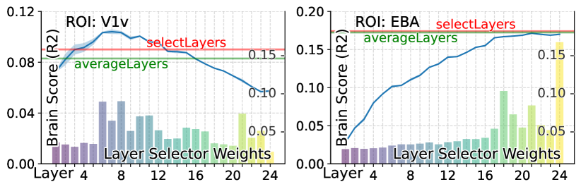
Figure 9: Grid search matched layer selector weights. Right y-axis is selector weights, and left y-axis is prediction score. Blue curve: per-layer model grid search score; Red line: score with layer selection; Green line: score with uniform layer average. Grid search with class token only.

Method	Time‡	MACs	Brain Score $R^{2}$ $\uparrow$ ($\pm$ 0.001)
			all	V1v	V3v	EBA
classToken	$\times$1	$\times$1	0.100	0.085	0.075	0.173
patchToken [31]	$\times$1	$\times$1	0.122	0.176	0.163	0.165
GNetViT [2]	$\times$94	$\times$17	0.124	0.174	0.146	0.174
FactorTopy (Ours)	$\times$3	$\times$1.2	0.132	0.205	0.179	0.175
- w/o topology	$\times$3	$\times$1.4	0.130	0.197	0.176	0.174
- no layer sel	$\times$3	$\times$1.2	0.125	0.181	0.162	0.174
- no space sel	$\times$3	$\times$1.2	0.117	0.094	0.089	0.175
- no scale sel	$\times$3	$\times$1.2	0.131	0.201	0.177	0.175
+ multiple sample	$\times$7	$\times$1.6	0.134	0.207	0.182	0.176

Table 3: Performance Ablation. Average of 3 runs. ^‡: wall-clock.

5.2 Limited Training Data

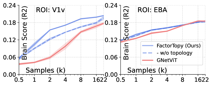
Figure 10: Performance w.r.t. training data sample, in log scale.

Practical use of our brain-to-network mapping tool for network visualization requires our network to be trained efficiently. Using data scaling experiments shown in Figure 10, we conclude that teaching our model with 3K sample images (30 minutes on RTX4090) offers a good trade-off. Our topological constraints and factorized feature selection (FactorTopy) scales better to less training data.

6 Discussion and Limitations

We have developed a visualization tool, FactorTopy, by training a robust brain encoding model. It allows us to see the internal working mechanism of any deep network. With this visualization and known functionality of brain ROIs, we can predict the network’s downstream task performance, and diagnose their behavior when scaling up with a larger model or finetuning to a small dataset. Our method is practical: only 3K images are needed to learn a visualization.

Limitation. High-quality brain-encoding data of input images paired with brain fMRI responses is needed. NSD is the only such data publicly available. Comparing brain-to-network alignments is less informative if networks’ computation differs entirely from the brain. It is possible to achieve efficiency in a non-brain-like way; therefore, our tool is not universally applicable to all network designs.

Figure 11: Brain Region of Interests (ROIs). Left: color is subject-specific ROI, and border overlay is subject-average common template ROIs. Right: subject-specific ROIs. V1v: ventral stream, V1d: dorsal stream.

ROI name	V1 V2 V3	V4	EBA FBA	OFA FFA	OPA	PPA	OWFA VWFA
Known Function/Selectivity	primary visual	mid-level	body	face	navigation	scene	words

Table 4: Known function and selectivity of brain region of interests (ROIs).

Appendix A Appendix Overview

1. Table 5 is an overview of key findings in this work.

2. Appendix B summarizes known function of brain ROIs.

3. Appendix C lists details of pre-trained models.

4. Appendix D is extended results with more ViT sizes, diffusion time steps, and more subjects.

5. Appendix E is implementation details of data processing and model training, pseudocode for visualization.

6. Appendix F summarizes state-of-the-art methods.

7. Appendix G demonstrates the resulting brain-to-network mapping when trained with less data samples.

A.1 Code Release

Code will be made publicly available upon publication. The pseudocode for our model and analysis is in Section E.2.

Appendix B Brain Region Details

This section briefly summarizes the known functionality of brain regions of interest (ROI). In our primary result, we included numerical results for V1, V2, V3, OPA, PPA, EBA, and FFA. In this appendix, we further report numerical results on FBA, OFA, OWFA, and VWFA.

Figure 11 is an overview of brain ROIs. We used subject-specific ROIs provided by NSD [2], NSD defined subject-specific ROIs by population receptive field (prf) and functional localizer (floc) experiments. It’s worth noting that common template ROIs are different from subject-specific ROIs.

Table 4 is known function and selectivity for each ROI. Briefly, V1 to V3 is the primary visual stream, they are further divided into ventral (lower) and dorsal (upper) streams. V4 is the mid-level visual area. EBA (extrastriate body area) and FBA (fusiform body area) are body-selective regions, FFA (fusiform face area) and OFA (occipital face area) are face-selective, OWFA (occipital word form area) and VWFA (visual word form area) are words selective. PPA (parahippocampal place area) is scene and place selective, and OPA (occipital place area) is related to navigation and spatial reasoning.

Key Observations	Sections	Figures & Tables
Brain Score
MAE and SAM are relatively better for the early visual brain, CLIP and DiNOv2 are relatively better for high-level brain regions.	4.1, D.1	Fig. 3; Tab. 1, 13
SD late time-steps are uniformly good for all brain regions.	4.1, D.1	Fig. 3; Tab. 1, 13
SD late time-steps are better for early brain, mid-to-late time steps are better for late brain.	D.1	Tab. 13
Brain-Net Alignment
Across all models included in this study, CLIP has the best brain-alignment.	4.2, 4.3	Fig. 4; Tab. 2
ImageNet and SAM last layer align to the mid-level visual brain, classification and segmentation are mid-level brain tasks.	4.2, D.2	Fig. 4, 15
DiNOv2 and MAE last layer does not align to any brain region, mask reconstruction deviates from the brain’s task.	4.2, D.2	Fig. 4, 15
MoCov3 last layers align better with the late ventral stream (‘what’ part) than the dorsal stream (‘what’ part), self contrastive learning is more on semantics than spatial relationship.	4.2, D.2	Fig. 4, 15
CLIP and ImageNet early layers align with the early visual brain, SAM DiNOv2 MAE MoCov3 early layers deviate from the brain.	4.2, D.2	Fig. 4, 14
SD have less separation in layers but more in time steps. SD encoder layers have more separation than decoder layers. SD’s brain-alignment is more ‘soft’ compared to ViT models. SD final time steps align to early brain regions, SD mid-late time steps align to the late brain.	4.2, D.2	Fig. 5, 16
Model Sizes
CLIP’s brain-net alignment improved as CLIP scaled up size and training data. In bigger CLIP models, both early and late layers become more aligned with the brain.	4.3, D.3	Fig. 4, 17
SAM, ImageNet, DiNOv2, MoCov3, and MAE’s brain-net alignment decreased as they scaled up sizes. ImageNet and DiNOv2 bigger models’ early layers deviate from the brain; SAM, MAE, and MoCov3 bigger models’ late layers deviate from the brain.	4.3, D.3	Fig. 4, 18-22
Fine-tuning
CLIP maintained brain-alignment after fine-tuning, DiNOv2 and MAE re-wired late layers.	4.4	Fig. 6
Fine-tuning performance does not correlate to change of computation layout, CLIP had the best fine-tuning performance but DiNOv2 and MAE also had competitive performance.	D.4	Tab. 14
Channels and Brain ROIs
Early visual brain uses similar channels but diverse spatial tokens. Late visual brain use diverse channels and global token.	4.5	Fig. 7, 2
The top selected channels reveal brain ROIs’ function. Image space features also reveal differences in various pre-trained models.	D.5	Fig. 8, 28-33
Methods and Consistency
Consistent subject difference exists in both brain prediction score and brain-net alignment.	D.1, 4.2	Fig. 12, 4; Tab. 13
Brain-Net mapping is consistent across random seeds within the same subject.	D.2	Fig. 13
Brain-Net mapping can be trained with limited training data samples. 3K data samples is a good trade-off for speed and quality.	5.2, G	Fig. 10, 27

Table 5: Overview of key observations in this work.

Appendix C Pre-trained Model Details

This section briefly summarizes the models included in this study. All the models are ViT architecture except for U-Net Stable Diffusion. We primarily used models released by their original authors, we used models from third-party releases when size variants are unavailable from the official release. We did not run any pre-training ourselves.

Model	Layers	Width	Input Size	Patch Size	Training Data
CLIP XL	24	1024	224x224	14x14	DataComp-1B
CLIP L	12	768	224x224	16x16	DataComp-140M
CLIP M	12	768	224x224	32x32	DataComp-14M
CLIP S	12	768	224x224	32x32	DataComp-1.4M

Table 6: CLIP Models.

CLIP

The objective of CLIP [44] (Contrastive Language-Image Pre-Training) is to match images with their corresponding text captions. The training objective is to minimize a contrastive loss that increases the similarity of paired images and text but decreases for unpaired ones. CLIP has two branches, one for vision and one for text, we only used the vision branch. We used a model released from the OpenCLIP [26] repository, models are pre-trained on data from DataComp [17]. Size variants of CLIP were trained on different sub-samples of data from 1B to 1.4M samples.

Model	Layers	Width	Input Size	Patch Size	Training Data
SAM H	32	1280	1024x1024	16x16	SA-1B
SAM L	24	1024	1024x1024	16x16	SA-1B
SAM B	12	768	1024x1024	16x16	SA-1B

Table 7: SAM Models.

SAM

The objective of the Segment Anything Model (SAM) [29] is interactive segmentation with points, boxes, or text prompts as additional input. SAM was trained without the class label of the objects, but the text prompts (CLIP embeddings) enhanced SAM’s understanding of the semantics. SAM was initialized from the MAE H model. Training was done on the SA-1B dataset, which was built by the SAM authors. SAM is an encoder-decoder design, we only took features from the encoder part. SAM’s ViT architecture does not have a class token, we used global averaging pooling to replace the global token. We used the officially released model weights for SAM.

ImageNet

This fully supervised model was trained to predict ImageNet [13] labels, the training was done on ImageNet-1K from scratch without any pre-training. We used model weights released by PyTorch Hub. We used a model from the improved training recipe that covers state-of-the-art training tricks and augmentations. Specifically, we used the IMAGENET1K_V1 weights, the base size model has 81.9 ImageNet accuracy, large size model has 79.7 accuracy.

Model	Layers	Width	Input Size	Patch Size	Training Data
ImageNet L	24	1024	224x224	16x16	IN-1K
ImageNet B	12	768	224x224	16x16	IN-1K

Table 8: ImageNet Models.

DiNOv2

The authors describe DiNOv2 [41] as DiNOv1 [6] plus iBOT [69] with the centering of SwAV [5]. DiNOv2 was trained with momentum self-distillation and mask reconstruction of latent tokens. The training was done on LVD-142M, which is a custom dataset made by the DiNOv2 authors. One notable difference to other models is that DiNOv2 smaller models were distilled from bigger models. We used the officially released model weights for DiNOv2.

Model	Layers	Width	Input Size	Patch Size	Training Data
DiNOv2 G	40	1536	224x224	14x14	LVD-142M
DiNOv2 L	24	1024	224x224	14x14	LVD-142M
DiNOv2 B	12	768	224x224	14x14	LVD-142M

Table 9: DiNOv2 Models.

MoCov3

The Momentum Contrastive (MoCo) [8] method trains contrastive loss with a momentum teacher encoder, which is an exponential moving average of the previous iteration models. The constrastive objective is to enforce the encoder to generate a similar representation to the momentum model. The training was done with the ImageNet-1K dataset. We used MoCov3 model weights released by MMPreTrain.

Model	Layers	Width	Input Size	Patch Size	Training Data
MoCov3 L	24	1024	224x224	16x16	IN-1K
MoCov3 B	12	768	224x224	16x16	IN-1K
MoCov3 S	12	384	224x224	16x16	IN-1K

Table 10: MoCov3 Models.

MAE

The Mask Autoencoder (MAE) [23] objective is to reconstruct the masked patches of input images given the un-masked patches, reconstruction is in the image space. The training was done on the ImageNet-1K dataset. MAE used an encoder and decoder design, we only studied the encoder part. We used the official release from the original authors.

Model	Layers	Width	Input Size	Patch Size	Training Data
MAE H	32	1280	224x224	16x16	IN-1K
MAE L	24	1024	224x224	16x16	IN-1K
MAE B	12	768	224x224	16x16	IN-1K

Table 11: MAE Models.

SD

The Stable Diffusion (SD) [46] model’s objective is to generate photo-realistic images. Although SD was trained without supervision on the loss term, the content of the generated image is controlled by a text prompt (CLIP embeddings), and the text prompt enhanced the semantic understanding of the features. SD is a U-Net and ResNet design with cross-attention to CLIP embeddings. There are 8 layers in the U-Net encoder and 12 layers in the decoder, skip connection connects the encoder and decoder blocks. There’s no class token in SD, we used global averaging pooling to replace it. In the feature extraction, we used an empty text prompt, we followed the ‘inversion’ time steps that chain the features of different time steps. SD was trained on LAION-5B [53] dataset. We used the Huggingface release of the SD version 1.5 model.

Encoder Layers	Decoder Layers	Width	Feature Size	Input Size	Training Data
1,2	10,11,12	320	64x64	512x512	LAION-5B
3,4	7,8,9	640	32x32	512x512	LAION-5B
5,6	4,5,6	1280	16x16	512x512	LAION-5B
7,8	1,2,3	1280	8x8	512x512	LAION-5B

Table 12: Stable Diffusion Layers.

Appendix D Extended Results

In addition to the main results in Section 4, this appendix presents extended results that cover more brain ROIs, more ViT model sizes, more diffusion time steps, and more subjects. The structure of this appendix section follows the main results:

1. Brain Score. Results on three subjects. Numerical results on more ROIs, all diffusion time steps.

2. Training Objectives and Brain-Net Alignment. Consistency check. Display of raw layer selector weights.

3. Network Hierarchy and Model Sizes. Layer selector results in more ViT model size variants.

4. Fine-tuned Models. Fine-tune performance score.

5. Channels and Brain ROIs. Top channel image feature display on more brain ROIs.

D.1 Brain Score

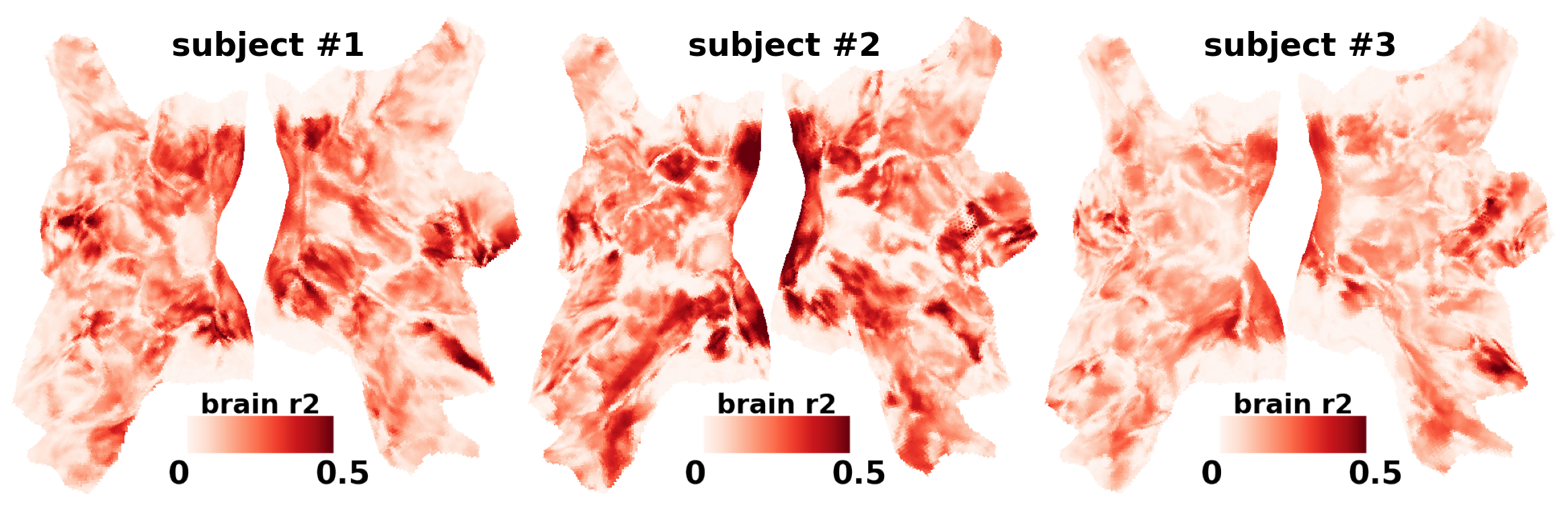
Figure 12: Brain Score. Three subjects, CLIP L (base size 12 layer) model.

	ROI Brain Score $R^{2}$ $\uparrow$ ($\pm$ 0.001)
Model	all	V1	V2	V3	V4	EBA	FBA	OFA	FFA	OPA	PPA	OWFA	VWFA
CLIP model, three subjects
CLIP (subject #1)	0.132	0.216	0.209	0.185	0.139	0.176	0.157	0.129	0.182	0.091	0.130	0.121	0.092
CLIP (subject #2)	0.154	0.247	0.183	0.192	0.188	0.182	0.134	0.098	0.136	0.126	0.199	0.083	0.140
CLIP (subject #3)	0.104	0.155	0.128	0.108	0.105	0.134	0.137	0.080	0.151	0.081	0.125	0.104	0.087
ViT models, subject #1
CLIP	0.132	0.216	0.209	0.185	0.139	0.176	0.157	0.129	0.182	0.091	0.130	0.121	0.092
SAM	0.110	0.212	0.197	0.172	0.113	0.127	0.120	0.104	0.142	0.074	0.104	0.105	0.066
ImageNet	0.120	0.205	0.202	0.174	0.127	0.159	0.143	0.117	0.169	0.076	0.121	0.109	0.077
DiNOv2	0.126	0.208	0.202	0.175	0.127	0.174	0.152	0.122	0.178	0.083	0.126	0.111	0.088
MAE	0.129	0.219	0.210	0.186	0.135	0.165	0.148	0.127	0.173	0.093	0.126	0.124	0.086
MoCov3	0.126	0.214	0.208	0.181	0.134	0.163	0.150	0.120	0.176	0.086	0.124	0.115	0.081
Stable Diffusion time steps, subject #1
T0	0.048	0.135	0.112	0.088	0.057	0.036	0.033	0.046	0.036	0.024	0.041	0.049	0.025
T5	0.062	0.151	0.130	0.103	0.070	0.053	0.050	0.055	0.056	0.039	0.055	0.058	0.033
T10	0.077	0.161	0.146	0.119	0.078	0.085	0.079	0.068	0.091	0.050	0.071	0.068	0.044
T15	0.095	0.187	0.169	0.141	0.097	0.111	0.105	0.085	0.123	0.063	0.090	0.083	0.055
T20	0.106	0.195	0.184	0.155	0.110	0.135	0.120	0.100	0.142	0.071	0.104	0.096	0.063
T25	0.112	0.199	0.191	0.161	0.109	0.149	0.127	0.109	0.151	0.076	0.112	0.103	0.068
T30	0.121	0.207	0.202	0.177	0.129	0.163	0.138	0.118	0.163	0.080	0.121	0.114	0.076
T35	0.125	0.212	0.205	0.178	0.128	0.170	0.145	0.123	0.169	0.084	0.126	0.118	0.083
T40	0.123	0.215	0.207	0.177	0.123	0.169	0.143	0.120	0.169	0.080	0.123	0.116	0.075
T45	0.125	0.215	0.208	0.181	0.130	0.170	0.145	0.124	0.170	0.082	0.125	0.119	0.078
T50	0.124	0.213	0.207	0.179	0.124	0.169	0.144	0.123	0.168	0.082	0.124	0.120	0.081

Table 13: Brain Score. ViT models are base size 12-layer. Bold marks best within each category, bold italic marks the second best. Top: CLIP model on three subjects. Middle: ViT models on subject #1. Bottom: Stable Diffusion model time steps on subject #1. Insights: 1) individual difference exists, subject #3’s early visual cortex is significantly less predictable. 2) CLIP and DiNOv2 are better for late brain regions, and MAE is better for the early visual cortex. 3) Stable Diffusion T35 is better for late brain regions, and T45 is better for early visual cortex.

In addition to the brain score reported in main results Section 4.1, we report 1) CLIP brain score on three subjects, 2) Numerical brain score results of ViT base size model on more ROIs, and 3) Stable Diffusion brain score results that cover the full time-step range. Notably, in main results 4.1 we reported the root summed square difference of brain score, in this appendix, we report the raw ROI-averaged brain score.

Three subjects

In Figure 12 and Table 13, subject #2 has a more predictable V1 while subject #3 has a least predictable early visual cortex. Subject #1 has a most predictable FFA and FBA. The prediction score difference matches the brain-to-network mapping results that subject #3 has large uncertainty in the early visual cortex (Figure 4), and subject #2 and #3 are missing the FFA region that subject #1 has. Overall, individual difference is expected and consistent.

ViT models

In Table 13, we report the raw ROI-average brain score. Among the ViT models, MAE has the best prediction power in early visual (V1 to V3) and navigation and spatial-relation region OPA. Interestingly, MAE has the best score in word and letter region OWFA but not for VWFA. CLIP has the best score in face, body, and scene-related regions (EBA, FBA, OFA, FFA, PPA) followed by DiNOv2.

Diffusion time steps

In Table 13, we report brain score fixing each diffusion time step. $T<25$ showed a sub-optimal performance score in all regions. $T=35$ showed the best performance on high-level regions (EBA, FBA, OPA, PPA), and $T=45$ showed good performance for all regions from early visual to high-level. Surprisingly, $T=0$ achieved relatively good brain score for the early visual ROIs.

D.2 Training Objectives and Brain-Net Alignment

In this section, we show: 1) consistency of brain-net alignment across random seeds, and 2) expanded raw layer selector weights.

Random seed consistency

In the main results Section 4.2 we found consistent differences across subjects. In this experiment, we repeated the same model and subject for 3 different random seeds. Results are in Figure 13, we found subjects #1 and #2 had consistent brain-to-layer mapping across random seeds. Subject #3 was less consistent across random seeds, note that subject #3 also had the lowest data quality (brain score, Table 13).

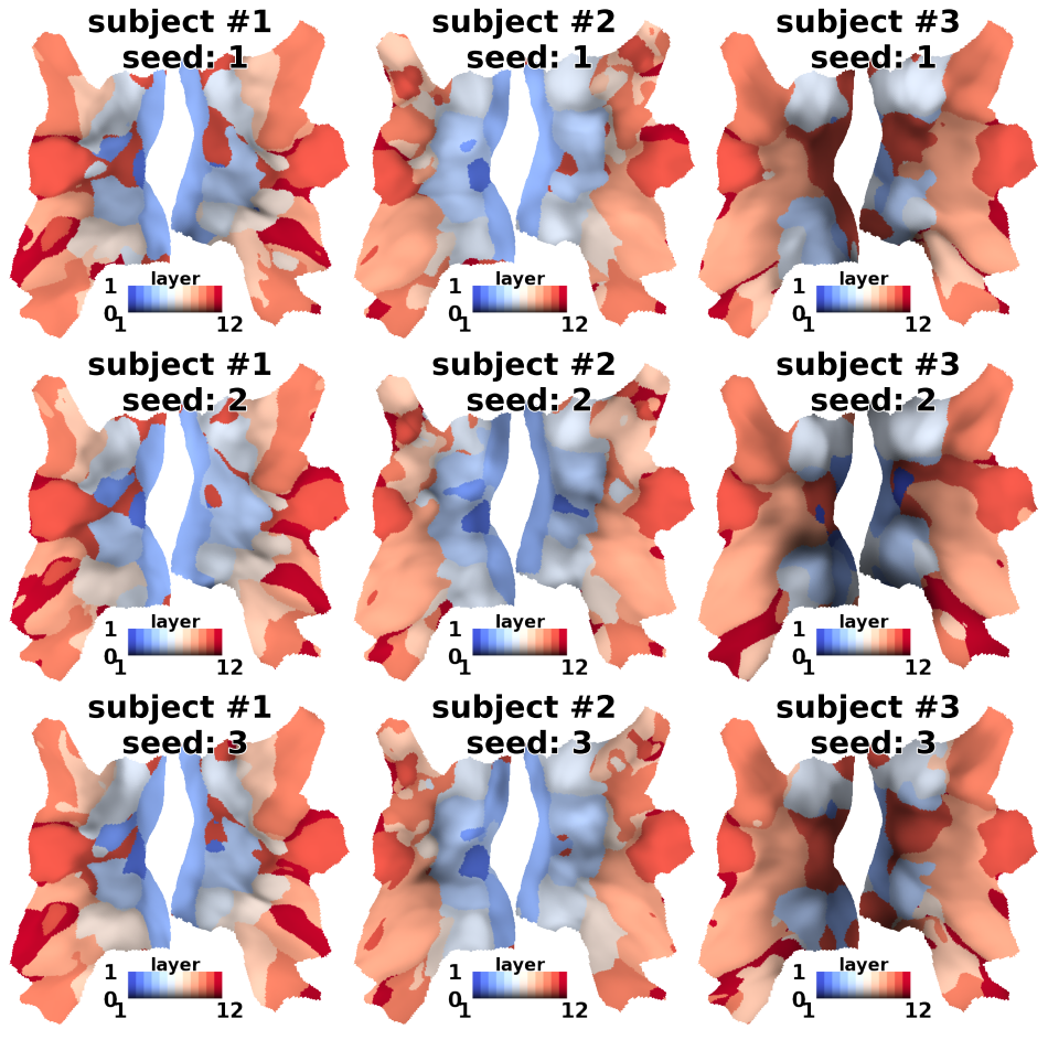
(a) CLIP

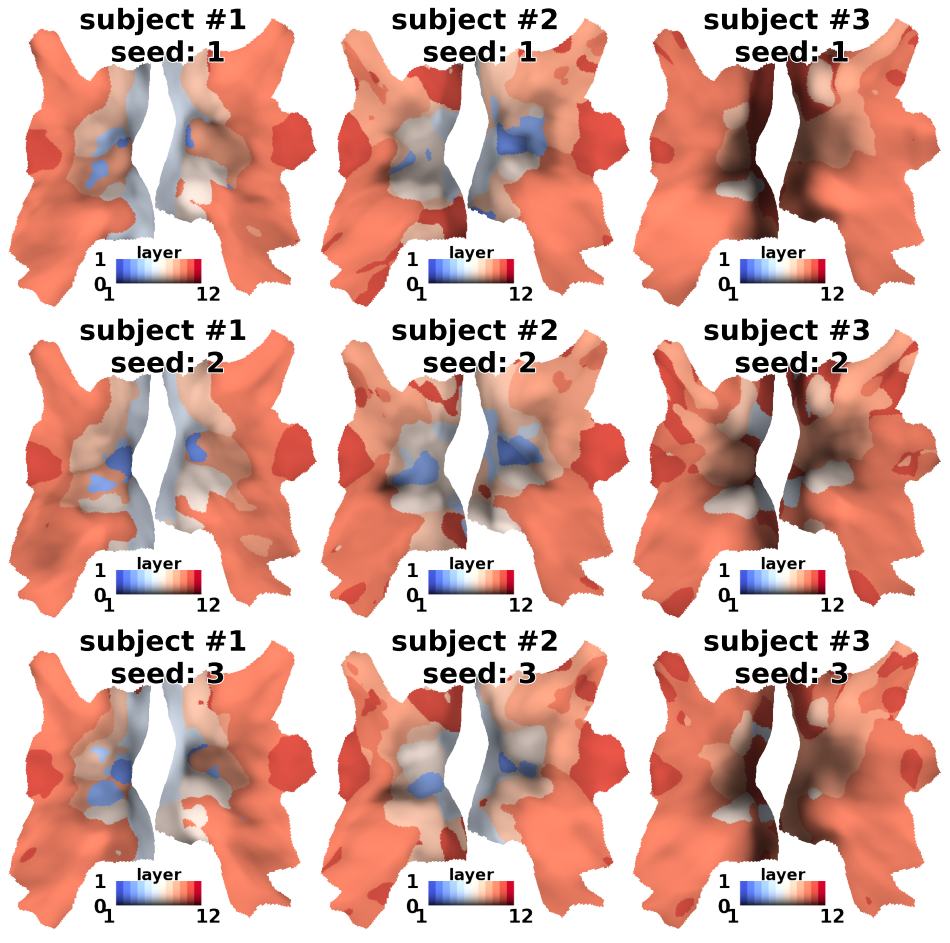
(b) MAE

Figure 13: Random Seed Consistency. CLIP (up) and MAE (down) model, 3 subjects (columns) and 3 random seeds (rows).

Raw layer selector weights

In our main results Sections 3.2 and 4.2, we displayed argmax and confidence of selected layers. In Figure 14-16, we display the raw output of layer selector weights for 1) 6 ViT base size 12-layer models, and 2) Stable Diffusion model fix time step T40 layer selection and fix decoder layer 6 time-step selection.

There are some interesting observations that are hard to conclude from the argmax plot but more visible in the raw weights: 1) CLIP layer 11 is strongly aligned to EBA but also weakly aligned to the mid-level dorsal stream. 2) ImageNet’s last layer is weakly aligned to all regions expect EBA and FFA. 3) SAM’s last layer is weakly aligned to the mid-to-high level dorsal stream and mid-level ventral stream. 4) DiNOv2’s last two layers’ alignment weakly follows layer 10. 5) MAE layer 10 strongly aligns to mid-to-high level dorsal and ventral stream, MAE last layer does not align to any brain regions. 6) MoCov3 layer 11 aligns with the late ventral stream but not the dorsal stream, and MoCov3’s layer 12 aligns with EBA.

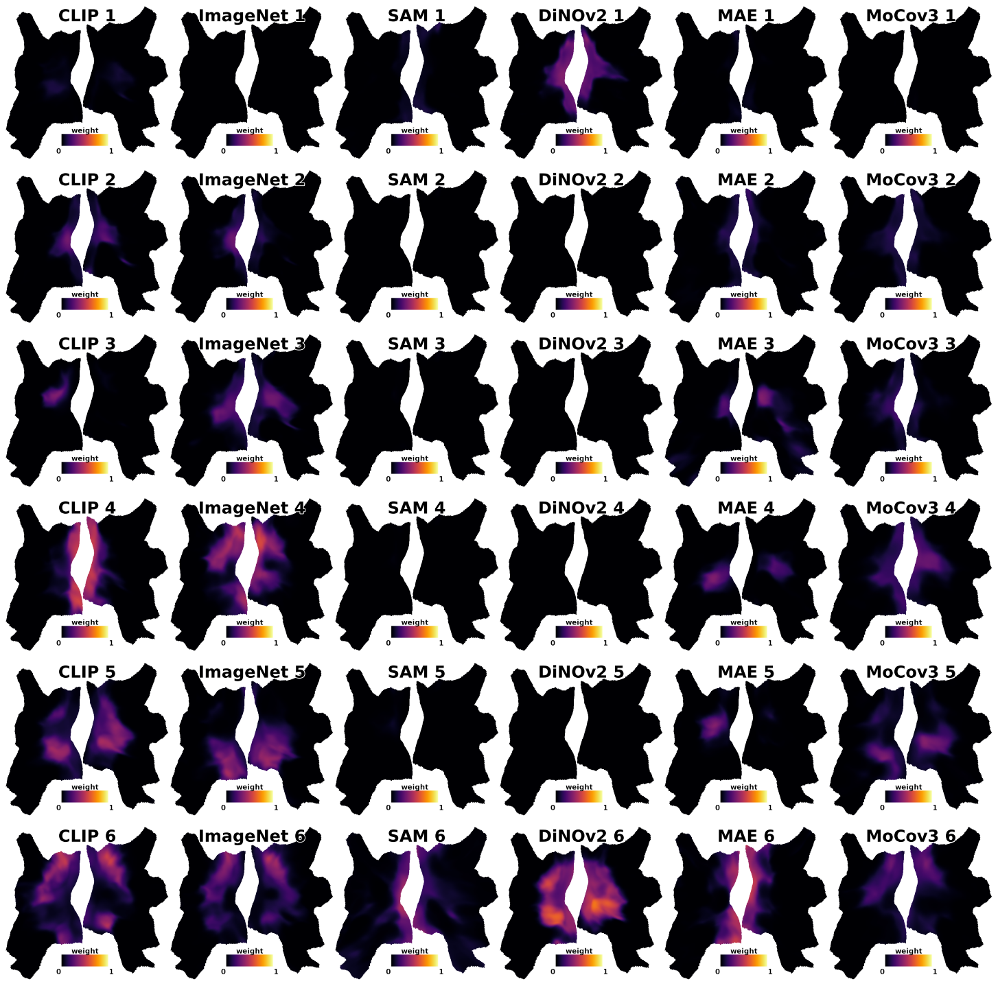
Figure 14: Raw Layer Selector weights (Part 1). Layer 1 to 6 of ViT base size 12-layer models. The number tailing model name is the layer index.

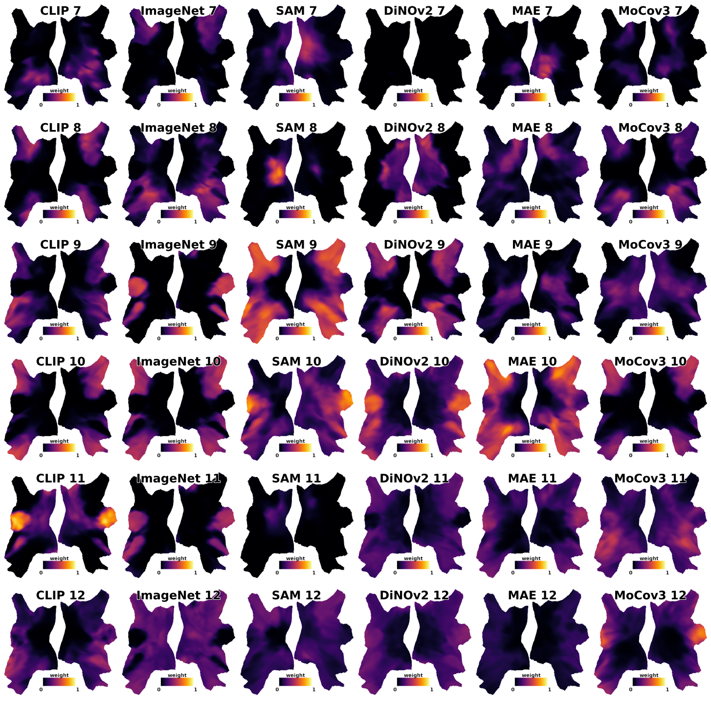
Figure 15: Raw Layer Selector weights (Part 2). Layer 7 to 12 of ViT base size 12-layer models. The number tailing model name is the layer index.

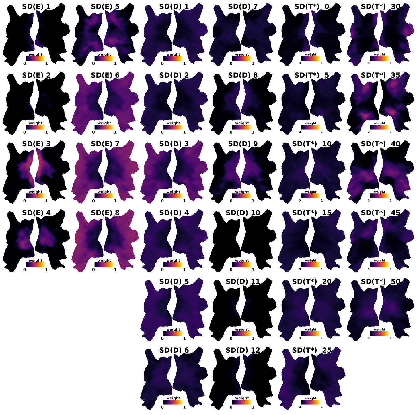
Figure 16: Raw Layer Selector weights (Part 3). Stable Diffusion model. SD(E): 8 encoder layers (fixed at T=40). SD(D): 12 decoder layers (fixed at T=40). SD(T*): 50 time steps (fixed at decoder layer no. 6). The number tailing model name is the layer or time step index.

D.3 Network Hierarchy and Model Sizes

In this section, we expand the main results Section 4.3 brain-layer alignment display to include more size variants. Details for pre-trained models, including layer, width, input size, patch size, and training data, are in Appendix C.

CLIP

CLIP models showed increasing brain-net alignment as they scaled up both data and size. Both early and late layers in larger CLIP models are more selected by the brain. Notable, CLIP (M) and CLIP (S) were trained with the same model size but $\times 10$ smaller training samples, CLIP (S) showed low confidence selection for the whole visual brain and only the late layers were more selected.

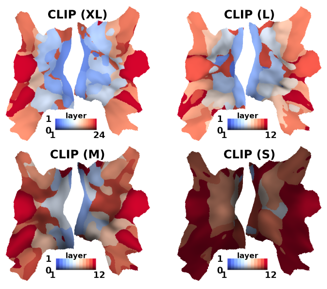
Figure 17: CLIP Brain-Net Alignment. XL to M are size and data variants, M and S are the same size but have smaller training data.

SAM

SAM models showed decreasing brain-net alignment as they scaled up sizes. Larger SAM models’ late layers were not selected; SAM’s early layers were not selected in all model sizes. The uncertainty of selection went up in the early visual cortex for larger SAM models.

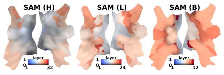
Figure 18: SAM Brain-Net Alignment. Size variants, same training data.

ImageNet

ImageNet models showed decreasing brain-net alignment as the size scales up. Base size ImageNet model’s early and late were both selected, larger size ImageNet model’s early layers were not selected.

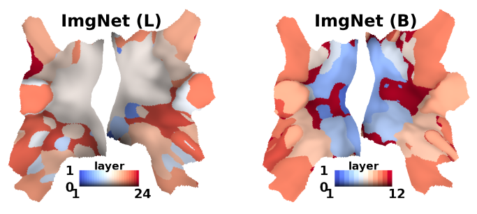
Figure 19: ImageNet Brain-Net Alignment. Size variants, same training data.

DiNOv2

DiNOv2 models showed decreasing brain-net alignment when scaled up. Larger DiNOv2 models’ early layers were less selected, only the last 1/4 of the layers were selected for the gigantic model. The first 1/2 of the layers were not selected for DiNOv2 models of all sizes.

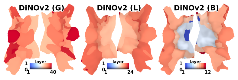
Figure 20: DiNOv2 Brain-Net Alignment. Size variants, same training data.

MAE

MAE models showed increasing brain-net alignment from base to large, decreasing from large to huge. MAE’s early layers were not selected for the base size model, selected for the large and huge size models. MAE’s late layers were not selected for the huge size model, selected for the base and large models. The huge model had more separation of semantic brain regions.

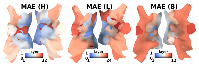
Figure 21: MAE Brain-Net Alignment. Size variants, same training data.

MoCov3

MoCov3 showed decreasing brain-net alignment as size scales up. MoCov3’s late layers were more selected for small and base size models, and MoCov3’s late layers were significantly less selected for large size models.

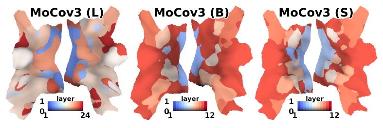
Figure 22: MoCov3 Brain-Net Alignment. Size variants, same training data.

D.4 Fine-tuned Model

In our main results Section 4.4, we showed brain-net mapping after fine-tuning. In this appendix, we report the fine-tuned performance score of each model.

Fine-tune last layer performance

In the main results Section 4.4, we attached an MLP prediction head to the last layer class token and fine-tuned the whole model to ISIC and EuroSAT tasks. In our main results, we found CLIP to maintain its brain-net alignment after fine-tuning while SAM and DiNOv2 re-wired their late layers.

In this appendix, we further reported the fine-tuning performance score in Table 14. CLIP had the best performance overall. Interestingly, SAM and DiNOv2 also had competitive performance despite their late layers being mostly re-wired (Section 4.4). We found the fine-tuning performance score does not correlate to the changes in brain alignments.

	Fine-tuned Accuracy $\uparrow$
Dataset	CLIP	MAE	SAM	DiNOv2
ISIC ($\pm 0.008$)	0.640	0.589	0.627	0.622
EuroSAT ($\pm 0.004$)	0.954	0.936	0.885	0.946

Table 14: Fine-tuned performance score. Average of 10 runs. The whole model is fine-tuned with the prediction head attached to the last layer class token.

Grid search on which layer to fine-tune

In the main results, we stated that “ISIC requires low-level features”, we verify this statement in this appendix. In this experiment, we ran a grid search that attached the prediction head to each layer, layers before the prediction layer are trained, and layers after the prediction layer are discarded. In Figure 23, on ISIC, we found CLIP layer 7 reached peak performance, and other models also peaked at mid-to-late layers; on EuroSAT, all models’ performance peaked at the last or second-last layer. Overall, the ISIC task relies on low-level features, EuroSAT task relies on high-level features.

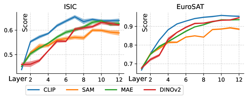
Figure 23: Grid search of fine-tuned layer. Average of 10 runs. The prediction head is attached to one layer, later layers are discarded.

D.5 Channels and Brain ROIS

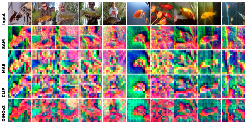
(a) V1 (early visual)

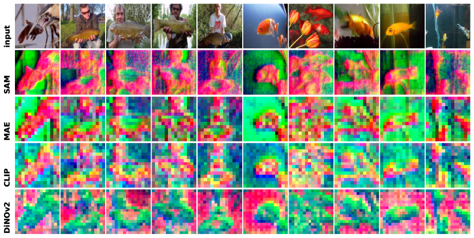
(b) V2 (early visual)

Figure 28: Top 3 selected channels for voxels in one brain ROI (methods in Section E.2, findings in Section D.5).

In the main results Section 4.5, we displayed the top selected channel in latent image space for V1 and FFA. In this appendix, we further display all ROIs: V1, V2, V3, V4, EBA, FBA, OFA, FFA, OPA, PPA, OWFA, and VWFA. Results are in Figure 28 to 33. Methods and pseudocode are in Section E.2.

Comparing across all ROIs, we found:

• from V1 to V4, features become increasingly abstract

• EBA captures the body but not including face, EBA has two global patterns for whether a human is present

• FBA captures body including face, FBA has two global patterns for whether a human is present

• OFA segments out object and background

• FFA reacts to face centered at the eyeball, FFA has two global patterns for whether a human is present

• OPA segments out the central object but not peripheral objects

• PPA reacts uniformly to the whole image

• OWFA segments out the object and background

• VWFA has two global patterns for whether a human is present

Comparing across all models, we found:

• SAM’s V1 to V4 features have finer segmentation of objects, SAM’s EBA activates less on bodies, SAM’s OPA does not capture the global layout, and SAM’s OWFA does not capture abstract representation.

• MAE’s EBA activates less on bodies, MAE’s FBA activates more on bodies and faces.

• CLIP’s V4 has less activation on the central object, CLIP’s EBA reacts to human bodies FBA reacts to animal bodies.

• DiNOv2’s V3 showed grid structure, DiNOv2’s EBA and FBA react to human bodies but less to animal bodies.

Appendix E Methods Details

E.1 NSD Data Processing Details

We used the officially released GLMsingle [43] beta3 preparation of the data, the pre-processing pipeline consists of motion correlation, hemodynamic response function (HRF) selection for each voxel, nuisance regressor estimation via PCA, and finally, a general linear model (GLM) is fit independently for each voxel with selected HRF and nuisance regressor. In addition to the officially released pre-processing, we applied session-wise z-score to each voxel independently [19]. We used the official release of the data on FreeSurfer average (brain surface) space. There’s a total of 327,684 vertices for the whole cerebral cortex and sub-cortical regions, we only used 37,984 vertices in the visual cortex defined by the ‘nsdgeneral’ ROI. We used coordinates of vertices in inflated brain surface space.

E.2 Model and Visualization Pseudocode Code

Model (FactorTopy) Pseudocode

Figure 24 presents a PyTorch-style pseudocode for our main FactorTopy model. The factorized selectors in Equation 1 are implemented as separate MLPs with tanh, softmax, and sigmoid activation functions, respectively. pe is sinusoidal positional encoding.

⬇

### FactorTopy model ###

# x: Tensor, [B, 3, 224, 224], B := batch size

# coord: Tensor, [N, 3], N := number of voxels

\par## 1. backbone

local_tokens, global_tokens = backbone(x)

# local_tokens: dict, {layer: [B, C, H, W]}

# global_tokens: dict, {layer: [B, C]}

\par## 2a. downsample, (H, W) -> (8, 8)

local_tokens = downsample(local_tokens)

\par## 2b. layer-unique bottleneck, C -> D

for layer in layers:

local_tokens[layer] = bottle_neck[layer](

local_tokens[layer]) # [B, D, 8, 8]

global_tokens[layer] = bottle_neck[layer](

global_tokens[layer]) # [B, D]

\par## 3. multi-selectors

space = tanh(space_mlp(pe(coord))) # [N, 2]

layer = softmax(layer_mlp(pe(coord))) # [N, L]

scale = sigmoid(scale_mlp(pe(coord))) # [N, 1]

\par## 4. get v

# get v_local

v_local = bilinear_interpolate(

local_tokens, space) # [B, N, D, L]

# sum v_local and v_global

v_global = stack(global_tokens).repeat(1, N)

# [B, N, D, L]

v = v_local * (1-scale) + v_global * scale

# [B, N, D, L]

# sum over layers

v = (v * layer).sum(dim=-1) # [B, N, D]

\par## 5. voxel-specific linear regression

y = (v * w).mean(dim=-1) + b # [B, N]

Figure 24: PyTorch-style pseudocode of our methods FactorTopy.

Channel Clustering

We clustered selected channels (linear regression weights $\bm{w}$) into 20 clusters in primary results Section 4.5 and Section D.5. The procedure for clustering is: 1) use kernel trick $\bm{\bar{w}}=\bm{w}^{T}\bm{w}$, $\bm{w}\in\mathbb{R}^{D\times N}$ where $D$ is channel dimension, $N$ is the number of voxels. 2) use k-means clustering on $\bm{\bar{w}}$ with euclidean distance, k=1000. 3) use Agglomerative Hierarchical Clustering on the k-means centroids, euclidean distance, and Ward’s method, iterative merge until resulting in 20 clusters.

Channel Visualization Pseudocode

In the main results Section 4.5 and Section D.5, we visualized the top selected channel in image space for brain ROIs. The motivation for the image space visualization is to plot the top selected channel for an ROI of voxels; voxels’ linear regression weights are functioning as ‘channel selection’ that answers “which channels best predict my brain response?”.

In a single voxel case, we can 1) obtain local tokens $\mathbb{R}^{D\times H\times W}$ by summing features $\mathbb{R}^{L\times D\times H\times W}$ with layer selector weight $\bm{\hat{\omega}}_{i}\in\mathbb{R}^{L}$, 2) sum local tokens $\mathbb{R}^{D\times H\times W}$ with regression weight $w_{i}\in\mathbb{R}^{D}$, output a greyscale image $\mathbb{R}^{1\times H\times W}$.

To extend to an ROI of voxels, we 1) summed local tokens from all layer $\mathbb{R}^{L\times D\times H\times W}$ by ROI-average layer selector weights $\bm{\hat{\omega}}_{*}=\frac{1}{|roi|}\sum_{i\in roi}\bm{\hat{\omega}}_{i}$, where $|roi|=N^{\prime}$, output $\mathbb{R}^{D\times H\times W}$, 2) applied PCA to reduce linear regression weights $\mathbb{R}^{D\times N^{\prime}}$ along the dimension of number of voxels $N^{\prime}$, output $\mathbb{R}^{D\times 3}$, 3) applied top 3 PC weights to local tokens to reduce the channel dimension $D$ of local tokens, output RGB image $\mathbb{R}^{3\times H\times W}$. A complete pseudocode is in Figure 25.

⬇

### top channel visualization ###

# x: Tensor, [3, 224, 224], batch size is 1

# coord: Tensor, [N, 3], N := number of voxels

# roi_mask: Tensor, [N], boolean, sum = N’

\par## 1. backbone

local_tokens, global_tokens = backbone(x)

# local_tokens: dict, {layer: [C, H, W]}

\par## 2b. layer-unique bottleneck, C -> D

for layer in layers:

local_tokens[layer] = bottle_neck[layer](

local_tokens[layer]) # [D, H, W]

local_tokens = stack(local_tokens)

# [L, D, H, W]

\par## 3. multi-selectors

layer = softmax(layer_mlp(pe(coord[roi_mask])))

# [N’, L]

\par## 4. sum local_tokens by ROI

layer_weights = layer.mean(0) # [L]

local_tokens = sum(layer_weights * local_tokens)

# [D, H, W]

\par## 5. PCA on linear regression weights

_w = w[:, roi_mask] # [D, N’]

_pc_w = pca(_w) # [D, 3]

\par## 6. RGB image

image = _pc_w.t() @ local_tokens # [3, H, W]

Figure 25: PyTorch-style pseudocode for channel visualization.

E.3 Training Details

Hardware and Wall-clock

We conducted experiments on a mixture of Nvidia A6000 and RTX4090 GPUs. Features of the pre-trained model are pre-computed and cached. We used bottleneck dimension $D=128$; increasing $D$ will significantly increase computation intensity as the number of brain voxels (vertices) is large (37,984). A full data (22K data samples) model converges in 1 to 3 hours for 12 to 40 layer models respectively. A partial data (3K data samples) 12-layer model converges in 30 minutes.

Optimizer and Training Recipe

For training brain encoding models, we used the AdamW optimizer, batch size 8, learning rate 1e-3, betas (0.9, 0.999), and weight decay 1e-2. We trained for 1,000 steps per epoch, with an early stopping of 20 epochs. Models reached maximum validation score at 40,000 to 60,000 steps, and the multi-selectors in our methods became stable after 10,000 steps. For each model, we saved the top 10 validation checkpoints and used ModelSoup [63] to average the best validation checkpoints and greedily optimize the score on the test set. We did not apply any data augmentation, existing data augmentation is not useful for brain encoding because the prediction target (brain) is not transformed alongside the input image.

Loss and Regularization

We used smooth L1 loss (beta=0.1) with an additional decaying regularization term on layer selector $\bm{\hat{\omega}}^{layer}$. The motivation for regularization is the use of softmax activation function in layer selector MLP leads to vanishing gradient at one-hot output, layer selector converges to a singular selection for all voxels (Figure 26) if with insufficient regularization,

$$loss_{reg} =-\frac{1}{N}\sum_{i=1}^{N}(\frac{\sum_{l=1}^{L}\hat{\omega}_{i,l}^{layer}\log\hat{\omega}_{i,l}^{layer}}{\sum_{l=1}^{L}\frac{1}{L}\log\frac{1}{L}})$$ (1)

$$decay =max(0,1-\frac{step_{i}}{step_{total}})$$

$$loss =loss_{l1}+\lambda*loss_{reg}*decay$$

$N$ is number of voxels, $L$ is number of layers, $\lambda$ is set to 0.1, $step_{i}$ is the current training step, $step_{total}$ is total steps of linear decaying. In Table 15, we ran a grid search of $step_{total}$ and concluded to use a total decay step of 6000; the same total decay step is set for all models. Figure 26 shows the resulting brain-to-layer mapping when trained with less regularization decay steps. When trained with insufficient regularization, layer selection converges to a local minimum (Table 15) of selecting only the last layer (Figure 26).

It’s worth noting that it’s possible to optimize the performance score by searching optimal decay steps for every model. However, we use entropy as a confidence measurement (Equation 2) in our experiments. The regularization term impacts the resulting confidence value, thus, we set the same total decay step (6000) for all models to avoid unfair comparison of confidence measurement.

	Decay Steps, Brain Score $R^{2}$ $\uparrow$ ($\pm$ 0.001)
Model	2000	4000	6000	8000
CLIP	0.093	0.128	0.131	0.132
DiNOv2	0.113	0.126	0.126	0.125

Table 15: Performance score w.r.t. total decay steps for regularization term. Grid search with CLIP and DiNOv2 base size 12-layer model. Average of 3 runs.

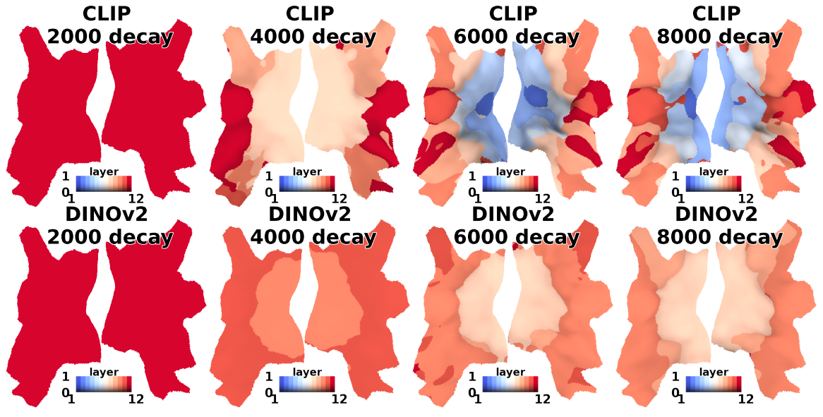
Figure 26: Layer selector output w.r.t. regularization decay total steps, number is total steps.

Appendix F Related Work: State-of-the-art Methods

In the main text Section 5.1, we compared our methods against the state-of-the-art methods’ most salient design, but not their original methods. In this appendix, we discuss the competition-winning approaches in detail and explain the motivation for comparing their most salient design but not their original methods.

Experiment Setting

Our experiment setting is different from the competition-winning methods. They build an ensemble of ROI-unique models, there’s less demand for voxel-wise feature selection in ROI-unique models because voxels in the same ROI select similar features. However, we build one all-ROI model that covers all visual brain voxels, and the local similarity and global diversity of voxels emphasized the importance of factorized and topology-constrained feature selection introduced in this work. Overall, existing work use pre-defined ROIs and ensemble of ROI-unique models, we build one all-ROI model.

Algonauts 2021 winner, patchToken

The Algonauts 2021 challenge was hosted with another 3T fMRI dataset [31] but not NSD. The Algonauts 2021 dataset lacks the high data quality that NSD has, the lower data quality limited the effect of novel model building. The Algonauts 2021 competition winners (the top 3 methods are summarized in supplementary of [31]) used primitive methods that do not select unique features for each voxel but compress the flattened patches into one feature vector for all voxels. All voxels use the same feature vector. The most salient design in Algonauts 2021 is the patch compression module, patchToken, we re-implemented their methods (Table 3, patchToken) and found that patchToken methods achieved sub-optimal performance on the high-quality dataset NSD.

GNet by NSD

Before the Algonauts 2023 challenge, for the NSD dataset, the commonly used state-of-the-art method is GNet introduced by the NSD authors [2]. GNet introduced a layer-specific spatial pooling field for each voxel, which is a non-factorized and non-topology-constrained feature selection for each voxel. The original GNet was an end-to-end CNN trained from scratch, later studies [12] swapped the image backbone model with frozen state-of-the-art pre-trained ViT models to increase the performance. In our comparison we used a frozen CLIP XL model for all the models, so it’s not the original GNet. The most salient design in GNet is the layer-specific spatial pooling field, we re-implemented the spatial pooling field design and compared it with our methods (Table 3, GNetViT). Notably, GNetViT requires quadratic memory and computation because of the unique $L\times H\times W$ spatial pooling field for each voxel.

Algonauts 2023 first place

Our methods is an extension of the Algonauts 2023 winning methods Memory Encoding Model (Mem) [67]. Mem used topology constraints but only partially factorized the feature selection (they are missing the scale axis). In our methods, we further introduced fully factorized feature selection. There are some major differences between our work and their settings: 1) We only consider one image as input, Mem used extra information including past 32 images, behavior response, and time information, extra information led to a shocking 10% challenge score boost. 2) We build one single all-ROI model, Mem builds an ensemble of ROI-unique models. 3) We ran the training only once, Mem used dark knowledge distillation and ran the training twice. 4) We only used voxels in the visual brain, Mem additionally used voxels outside the visual brain to increase data samples. 5) We only used one subject for training, Mem trained a shared backbone for all 8 subjects. Mem’s is partially factorized (without scale axis) and topology-constrained feature selection, we included Mem’s most salient design in our ablation study in Table 3 “- no scale sel”.

Algonauts 2023 second place

For the second place winning methods of the Algonauts 2023 challenge [1], the most important factors to their winning are: 1) they used extra information including behavior response and time information, which led to a 4% challenge score boost, 2) they built ROI-unique models ensemble, and 3) they trained on 8 subjects. For the methods, they used a Detection Transformer (DETR) style attention mask with ROIs as queries. Their feature selection is voxel-shared but ROI-specific and also image-specific, not factorized or topology constrained. The DETR-style attention mask requires quadratic computation resources, their methods is possible to run for 36 ROIs as queries but impossible for 37,984 voxels as queries. We did not include the transformer methods in the comparison because their methods fundamentally rely on pre-defined ROIs and are unable to scale up to voxels. The closest comparison to this transformer method is GNetViT.

Algonauts 2023 third place

For the third place winning methods of the Algonauts 2023 challenge [39], the most important factors that contributed to their winning are: 1) they ensembled 6 backbone models, 2) they pre-trained models on all ROI and all subjects, then fine-tuned ROI-unique models for each subject, and 3) they used a bag of training tricks. Their method used the same feature vector for voxels in the same ROI, similar to the patchToken methods in Algonauts 2021. However, it remains unclear how they compressed the $L\times C\times H\times W$ feature into one feature vector. We did not include this method in the comparison because the feature compression module is unclear, the closest comparison is classToken and patchToken.

Figure 27: Brain-to-Network alignment trained with limited data samples. Base size models, number of samples marked in brackets.

Appendix G Limited Training Samples

Practical use of our brain-to-network mapping as a debugging and visualization tool requires training with less data. In addition to data scaling performance reported in Section 5.2, we display the resulting brain-to-network mapping in Figure 27. We conclude that teaching our model with 3K single-trail sample images offers a good trade-off.

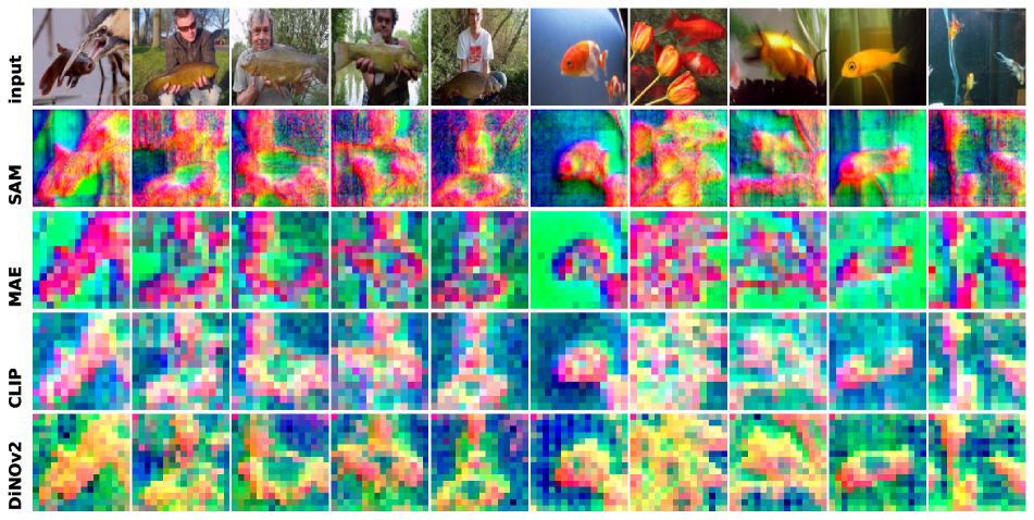
(a) V3 (early visual)

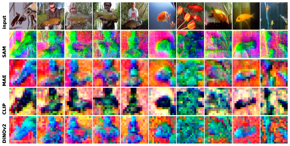
(b) V4 (mid-level)

Figure 29: Top 3 selected channels for voxels in one brain ROI (methods in Section E.2, findings in Section D.5).

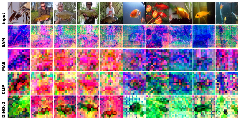
(a) EBA (body)

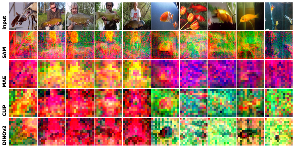
(b) FBA (body)

Figure 30: Top 3 selected channels for voxels in one brain ROI (methods in Section E.2, findings in Section D.5).

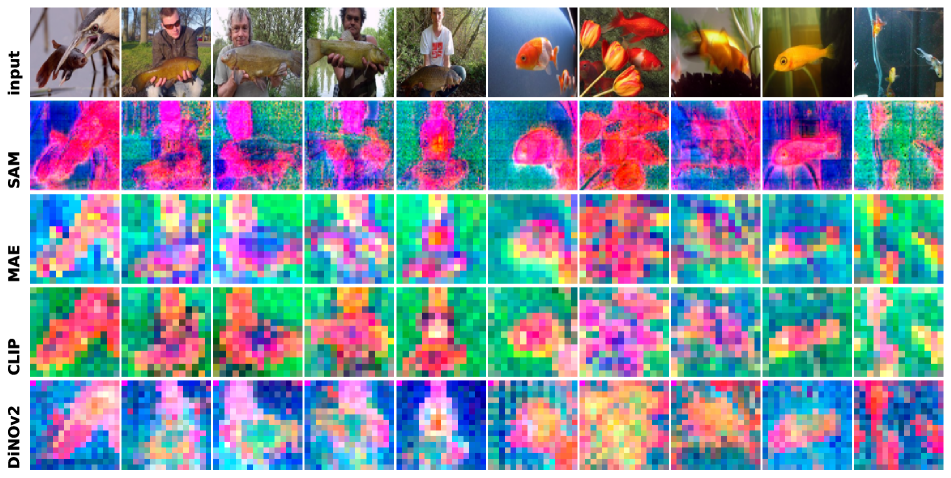
(a) OFA (face)

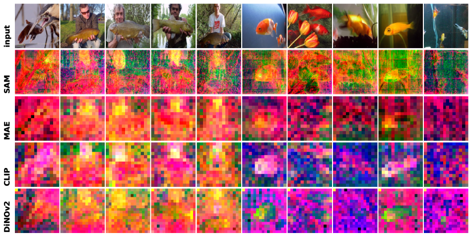
(b) FFA (face)

Figure 31: Top 3 selected channels for voxels in one brain ROI (methods in Section E.2, findings in Section D.5).

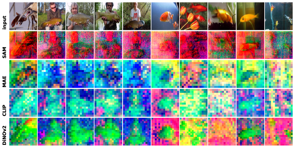
(a) OPA (navigation)

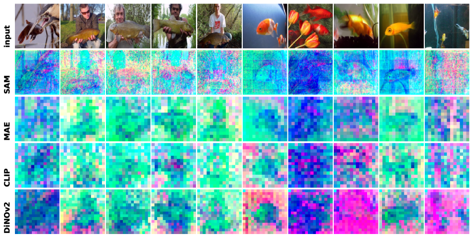
(b) PPA (scene)

Figure 32: Top 3 selected channels for voxels in one brain ROI (methods in Section E.2, findings in Section D.5).

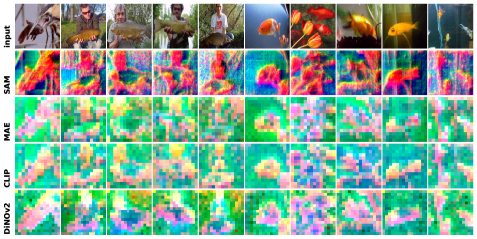
(a) OWFA (words)

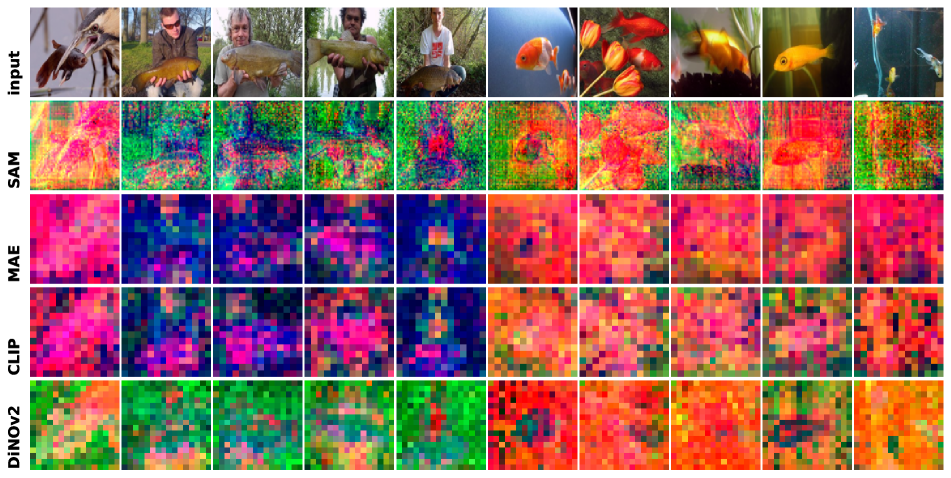
(b) VWFA (words)

Figure 33: Top 3 selected channels for voxels in one brain ROI (methods in Section E.2, findings in Section D.5).

References

- [1] Hossein Adeli, Sun Minni, and Nikolaus Kriegeskorte. Predicting brain activity using Transformers, Aug. 2023. Pages: 2023.08.02.551743 Section: New Results.
- [2] Emily J. Allen, Ghislain St-Yves, Yihan Wu, Jesse L. Breedlove, Jacob S. Prince, Logan T. Dowdle, Matthias Nau, Brad Caron, Franco Pestilli, Ian Charest, J. Benjamin Hutchinson, Thomas Naselaris, and Kendrick Kay. A massive 7T fMRI dataset to bridge cognitive neuroscience and artificial intelligence. Nature Neuroscience, 25(1):116–126, Jan. 2022. Number: 1 Publisher: Nature Publishing Group.
- [3] Martin Arjovsky, Soumith Chintala, and Léon Bottou. Wasserstein GAN, Dec. 2017. arXiv:1701.07875 [cs, stat].
- [4] Pouya Bashivan, Kohitij Kar, and James J. DiCarlo. Neural population control via deep image synthesis. Science, 364(6439):eaav9436, May 2019. Publisher: American Association for the Advancement of Science.
- [5] Mathilde Caron, Ishan Misra, Julien Mairal, Priya Goyal, Piotr Bojanowski, and Armand Joulin. Unsupervised Learning of Visual Features by Contrasting Cluster Assignments, Jan. 2021. arXiv:2006.09882 [cs].
- [6] Mathilde Caron, Hugo Touvron, Ishan Misra, Hervé Jégou, Julien Mairal, Piotr Bojanowski, and Armand Joulin. Emerging Properties in Self-Supervised Vision Transformers, May 2021. arXiv:2104.14294 [cs].
- [7] Nadine Chang, John A. Pyles, Austin Marcus, Abhinav Gupta, Michael J. Tarr, and Elissa M. Aminoff. BOLD5000, a public fMRI dataset while viewing 5000 visual images. Scientific Data, 6(1):49, May 2019. Number: 1 Publisher: Nature Publishing Group.
- [8] Xinlei Chen, Saining Xie, and Kaiming He. An Empirical Study of Training Self-Supervised Vision Transformers, Aug. 2021. arXiv:2104.02057 [cs].
- [9] R. M. Cichy, K. Dwivedi, B. Lahner, A. Lascelles, P. Iamshchinina, M. Graumann, A. Andonian, N. A. R. Murty, K. Kay, G. Roig, and A. Oliva. The Algonauts Project 2021 Challenge: How the Human Brain Makes Sense of a World in Motion, Apr. 2021. arXiv:2104.13714 [cs, q-bio].
- [10] Radoslaw Martin Cichy, Gemma Roig, Alex Andonian, Kshitij Dwivedi, Benjamin Lahner, Alex Lascelles, Yalda Mohsenzadeh, Kandan Ramakrishnan, and Aude Oliva. The Algonauts Project: A Platform for Communication between the Sciences of Biological and Artificial Intelligence, May 2019. arXiv:1905.05675 [cs, q-bio].
- [11] Noel Codella, Veronica Rotemberg, Philipp Tschandl, M. Emre Celebi, Stephen Dusza, David Gutman, Brian Helba, Aadi Kalloo, Konstantinos Liopyris, Michael Marchetti, Harald Kittler, and Allan Halpern. Skin Lesion Analysis Toward Melanoma Detection 2018: A Challenge Hosted by the International Skin Imaging Collaboration (ISIC), Mar. 2019. arXiv:1902.03368 [cs].
- [12] Colin Conwell, Jacob S. Prince, Kendrick N. Kay, George A. Alvarez, and Talia Konkle. What can 1.8 billion regressions tell us about the pressures shaping high-level visual representation in brains and machines?, July 2023. Pages: 2022.03.28.485868 Section: New Results.
- [13] Jia Deng, Wei Dong, Richard Socher, Li-Jia Li, Kai Li, and Li Fei-Fei. ImageNet: A large-scale hierarchical image database. In 2009 IEEE Conference on Computer Vision and Pattern Recognition, pages 248–255, June 2009. ISSN: 1063-6919.
- [14] James J. DiCarlo, Davide Zoccolan, and Nicole C. Rust. How does the brain solve visual object recognition? Neuron, 73(3):415–434, Feb. 2012.
- [15] Serge O. Dumoulin and Brian A. Wandell. Population receptive field estimates in human visual cortex. NeuroImage, 39(2):647–660, Jan. 2008.
- [16] Katrin Franke, Konstantin F. Willeke, Kayla Ponder, Mario Galdamez, Na Zhou, Taliah Muhammad, Saumil Patel, Emmanouil Froudarakis, Jacob Reimer, Fabian H. Sinz, and Andreas S. Tolias. State-dependent pupil dilation rapidly shifts visual feature selectivity. Nature, 610(7930):128–134, Oct. 2022. Number: 7930 Publisher: Nature Publishing Group.
- [17] Samir Yitzhak Gadre, Gabriel Ilharco, Alex Fang, Jonathan Hayase, Georgios Smyrnis, Thao Nguyen, Ryan Marten, Mitchell Wortsman, Dhruba Ghosh, Jieyu Zhang, Eyal Orgad, Rahim Entezari, Giannis Daras, Sarah Pratt, Vivek Ramanujan, Yonatan Bitton, Kalyani Marathe, Stephen Mussmann, Richard Vencu, Mehdi Cherti, Ranjay Krishna, Pang Wei Koh, Olga Saukh, Alexander Ratner, Shuran Song, Hannaneh Hajishirzi, Ali Farhadi, Romain Beaumont, Sewoong Oh, Alex Dimakis, Jenia Jitsev, Yair Carmon, Vaishaal Shankar, and Ludwig Schmidt. DataComp: In search of the next generation of multimodal datasets, Oct. 2023. arXiv:2304.14108 [cs].
- [18] Alessandro T. Gifford, Kshitij Dwivedi, Gemma Roig, and Radoslaw M. Cichy. A large and rich EEG dataset for modeling human visual object recognition. NeuroImage, 264:119754, Dec. 2022.
- [19] A. T. Gifford, B. Lahner, S. Saba-Sadiya, M. G. Vilas, A. Lascelles, A. Oliva, K. Kay, G. Roig, and R. M. Cichy. The Algonauts Project 2023 Challenge: How the Human Brain Makes Sense of Natural Scenes, Jan. 2023. arXiv:2301.03198 [cs, q-bio].
- [20] Zijin Gu, Keith Wakefield Jamison, Meenakshi Khosla, Emily J. Allen, Yihan Wu, Ghislain St-Yves, Thomas Naselaris, Kendrick Kay, Mert R. Sabuncu, and Amy Kuceyeski. NeuroGen: Activation optimized image synthesis for discovery neuroscience. NeuroImage, 247:118812, Feb. 2022.
- [21] Kamal Gupta, Gowthami Somepalli, Anubhav Anubhav, Vinoj Yasanga Jayasundara Magalle Hewa, Matthias Zwicker, and Abhinav Shrivastava. PatchGame: Learning to Signal Mid-level Patches in Referential Games. In Advances in Neural Information Processing Systems, volume 34, pages 26015–26027. Curran Associates, Inc., 2021.
- [22] Matthew Gwilliam and Abhinav Shrivastava. Beyond Supervised vs. Unsupervised: Representative Benchmarking and Analysis of Image Representation Learning. pages 9642–9652, 2022.
- [23] Kaiming He, Xinlei Chen, Saining Xie, Yanghao Li, Piotr Dollár, and Ross Girshick. Masked Autoencoders Are Scalable Vision Learners, Dec. 2021. arXiv:2111.06377 [cs].
- [24] Martin N Hebart, Oliver Contier, Lina Teichmann, Adam H Rockter, Charles Y Zheng, Alexis Kidder, Anna Corriveau, Maryam Vaziri-Pashkam, and Chris I Baker. THINGS-data, a multimodal collection of large-scale datasets for investigating object representations in human brain and behavior. eLife, 12:e82580, Feb. 2023. Publisher: eLife Sciences Publications, Ltd.
- [25] Patrick Helber, Benjamin Bischke, Andreas Dengel, and Damian Borth. EuroSAT: A Novel Dataset and Deep Learning Benchmark for Land Use and Land Cover Classification, Feb. 2019. arXiv:1709.00029 [cs].
- [26] Gabriel Ilharco, Mitchell Wortsman, Nicholas Carlini, Rohan Taori, Achal Dave, Vaishaal Shankar, Hongseok Namkoong, John Miller, Hannaneh Hajishirzi, Ali Farhadi, and Ludwig Schmidt. OpenCLIP, July 2021.
- [27] Ayush Jain, Nikolaos Gkanatsios, Ishita Mediratta, and Katerina Fragkiadaki. Bottom Up Top Down Detection Transformers for Language Grounding in Images and Point Clouds. In Shai Avidan, Gabriel Brostow, Moustapha Cissé, Giovanni Maria Farinella, and Tal Hassner, editors, Computer Vision – ECCV 2022, Lecture Notes in Computer Science, pages 417–433, Cham, 2022. Springer Nature Switzerland.
- [28] Nidhi Jain, Aria Wang, Margaret M. Henderson, Ruogu Lin, Jacob S. Prince, Michael J. Tarr, and Leila Wehbe. Selectivity for food in human ventral visual cortex. Communications Biology, 6(1):1–14, Feb. 2023. Number: 1 Publisher: Nature Publishing Group.
- [29] Alexander Kirillov, Eric Mintun, Nikhila Ravi, Hanzi Mao, Chloe Rolland, Laura Gustafson, Tete Xiao, Spencer Whitehead, Alexander C. Berg, Wan-Yen Lo, Piotr Dollár, and Ross Girshick. Segment Anything, Apr. 2023. arXiv:2304.02643 [cs].
- [30] Reese Kneeland, Jordyn Ojeda, Ghislain St-Yves, and Thomas Naselaris. Second Sight: Using brain-optimized encoding models to align image distributions with human brain activity, June 2023. arXiv:2306.00927 [cs, q-bio].
- [31] Benjamin Lahner, Kshitij Dwivedi, Polina Iamshchinina, Monika Graumann, Alex Lascelles, Gemma Roig, Alessandro Thomas Gifford, Bowen Pan, SouYoung Jin, N. Apurva Ratan Murty, Kendrick Kay, Aude Oliva, and Radoslaw Cichy. BOLD Moments: modeling short visual events through a video fMRI dataset and metadata, Mar. 2023. Pages: 2023.03.12.530887 Section: New Results.
- [32] Shamit Lal, Mihir Prabhudesai, Ishita Mediratta, Adam W. Harley, and Katerina Fragkiadaki. CoCoNets: Continuous Contrastive 3D Scene Representations. pages 12487–12496, 2021.
- [33] Tsung-Yi Lin, Michael Maire, Serge Belongie, Lubomir Bourdev, Ross Girshick, James Hays, Pietro Perona, Deva Ramanan, C. Lawrence Zitnick, and Piotr Dollár. Microsoft COCO: Common Objects in Context, Feb. 2015. arXiv:1405.0312 [cs].
- [34] Andrew F. Luo, Margaret M. Henderson, Michael J. Tarr, and Leila Wehbe. BrainSCUBA: Fine-Grained Natural Language Captions of Visual Cortex Selectivity, Oct. 2023. arXiv:2310.04420 [cs, q-bio].
- [35] Andrew F. Luo, Leila Wehbe, Michael J. Tarr, and Margaret M. Henderson. Neural Selectivity for Real-World Object Size In Natural Images, Mar. 2023. Pages: 2023.03.17.533179 Section: New Results.
- [36] Grace Luo, Lisa Dunlap, Dong Huk Park, Aleksander Holynski, and Trevor Darrell. Diffusion Hyperfeatures: Searching Through Time and Space for Semantic Correspondence, May 2023. arXiv:2305.14334 [cs].
- [37] Konstantin-Klemens Lurz, Mohammad Bashiri, Konstantin Willeke, Akshay Jagadish, Eric Wang, Edgar Y. Walker, Santiago A. Cadena, Taliah Muhammad, Erick Cobos, Andreas S. Tolias, Alexander S. Ecker, and Fabian H. Sinz. Generalization in data-driven models of primary visual cortex. Jan. 2021.
- [38] Ben Mildenhall, Pratul P. Srinivasan, Matthew Tancik, Jonathan T. Barron, Ravi Ramamoorthi, and Ren Ng. NeRF: Representing Scenes as Neural Radiance Fields for View Synthesis, Aug. 2020. arXiv:2003.08934 [cs].
- [39] Xuan-Bac Nguyen, Xudong Liu, Xin Li, and Khoa Luu. The Algonauts Project 2023 Challenge: UARK-UAlbany Team Solution, July 2023. arXiv:2308.00262 [cs].
- [40] Thomas P. O’Connell, Tyler Bonnen, Yoni Friedman, Ayush Tewari, Josh B. Tenenbaum, Vincent Sitzmann, and Nancy Kanwisher. Approaching human 3D shape perception with neurally mappable models, Sept. 2023. arXiv:2308.11300 [cs].
- [41] Maxime Oquab, Timothée Darcet, Théo Moutakanni, Huy Vo, Marc Szafraniec, Vasil Khalidov, Pierre Fernandez, Daniel Haziza, Francisco Massa, Alaaeldin El-Nouby, Mahmoud Assran, Nicolas Ballas, Wojciech Galuba, Russell Howes, Po-Yao Huang, Shang-Wen Li, Ishan Misra, Michael Rabbat, Vasu Sharma, Gabriel Synnaeve, Hu Xu, Hervé Jegou, Julien Mairal, Patrick Labatut, Armand Joulin, and Piotr Bojanowski. DINOv2: Learning Robust Visual Features without Supervision, Apr. 2023. arXiv:2304.07193 [cs].
- [42] Jacob S. Prince, George A. Alvarez, and Talia Konkle. A contrastive coding account of category selectivity in the ventral visual stream, Aug. 2023. Pages: 2023.08.04.551888 Section: New Results.
- [43] Jacob S. Prince, Ian Charest, Jan W. Kurzawski, John A. Pyles, Michael J. Tarr, and Kendrick N. Kay. Improving the accuracy of single-trial fMRI response estimates using GLMsingle. eLife, 11:e77599, Nov. 2022.
- [44] Alec Radford, Jong Wook Kim, Chris Hallacy, Aditya Ramesh, Gabriel Goh, Sandhini Agarwal, Girish Sastry, Amanda Askell, Pamela Mishkin, Jack Clark, Gretchen Krueger, and Ilya Sutskever. Learning Transferable Visual Models From Natural Language Supervision, Feb. 2021. arXiv:2103.00020 [cs].
- [45] N. Apurva Ratan Murty, Pouya Bashivan, Alex Abate, James J. DiCarlo, and Nancy Kanwisher. Computational models of category-selective brain regions enable high-throughput tests of selectivity. Nature Communications, 12(1):5540, Sept. 2021. Number: 1 Publisher: Nature Publishing Group.
- [46] Robin Rombach, Andreas Blattmann, Dominik Lorenz, Patrick Esser, and Björn Ommer. High-Resolution Image Synthesis with Latent Diffusion Models, Apr. 2022. arXiv:2112.10752 [cs].
- [47] Zvi N. Roth, Kendrick Kay, and Elisha P. Merriam. Natural scene sampling reveals reliable coarse-scale orientation tuning in human V1. Nature Communications, 13(1):6469, Oct. 2022. Number: 1 Publisher: Nature Publishing Group.
- [48] Gabriel Sarch, Zhaoyuan Fang, Adam W. Harley, Paul Schydlo, Michael J. Tarr, Saurabh Gupta, and Katerina Fragkiadaki. TIDEE: Tidying Up Novel Rooms Using Visuo-Semantic Commonsense Priors. In Shai Avidan, Gabriel Brostow, Moustapha Cissé, Giovanni Maria Farinella, and Tal Hassner, editors, Computer Vision – ECCV 2022, Lecture Notes in Computer Science, pages 480–496, Cham, 2022. Springer Nature Switzerland.
- [49] Gabriel Sarch, Hsiao-Yu Fish Tung, Aria Wang, Jacob Prince, and Michael Tarr. 3D View Prediction Models of the Dorsal Visual Stream, Sept. 2023. arXiv:2309.01782 [cs, q-bio].
- [50] Gabriel H. Sarch, Michael J. Tarr, Katerina Fragkiadaki, and Leila Wehbe. Brain Dissection: fMRI-trained Networks Reveal Spatial Selectivity in the Processing of Natural Images, May 2023. Pages: 2023.05.29.542635 Section: New Results.
- [51] Martin Schrimpf, Jonas Kubilius, Ha Hong, Najib J. Majaj, Rishi Rajalingham, Elias B. Issa, Kohitij Kar, Pouya Bashivan, Jonathan Prescott-Roy, Kailyn Schmidt, Daniel L. K. Yamins, and James J. DiCarlo. Brain-Score: Which Artificial Neural Network for Object Recognition is most Brain-Like?, Sept. 2018. Pages: 407007 Section: New Results.
- [52] Martin Schrimpf, Jonas Kubilius, Michael J. Lee, N. Apurva Ratan Murty, Robert Ajemian, and James J. DiCarlo. Integrative Benchmarking to Advance Neurally Mechanistic Models of Human Intelligence. Neuron, 108(3):413–423, Nov. 2020.
- [53] Christoph Schuhmann, Romain Beaumont, Richard Vencu, Cade Gordon, Ross Wightman, Mehdi Cherti, Theo Coombes, Aarush Katta, Clayton Mullis, Mitchell Wortsman, Patrick Schramowski, Srivatsa Kundurthy, Katherine Crowson, Ludwig Schmidt, Robert Kaczmarczyk, and Jenia Jitsev. LAION-5B: An open large-scale dataset for training next generation image-text models, Oct. 2022. arXiv:2210.08402 [cs].
- [54] Mannat Singh, Laura Gustafson, Aaron Adcock, Vinicius de Freitas Reis, Bugra Gedik, Raj Prateek Kosaraju, Dhruv Mahajan, Ross Girshick, Piotr Dollár, and Laurens van der Maaten. Revisiting Weakly Supervised Pre-Training of Visual Perception Models, Apr. 2022. arXiv:2201.08371 [cs].
- [55] Yu Takagi and Shinji Nishimoto. High-resolution image reconstruction with latent diffusion models from human brain activity, Nov. 2022. Pages: 2022.11.18.517004 Section: New Results.
- [56] Luming Tang, Menglin Jia, Qianqian Wang, Cheng Perng Phoo, and Bharath Hariharan. Emergent Correspondence from Image Diffusion, June 2023. arXiv:2306.03881 [cs].
- [57] JohnMark Taylor and Nikolaus Kriegeskorte. Extracting and visualizing hidden activations and computational graphs of PyTorch models with TorchLens. Scientific Reports, 13(1):14375, Sept. 2023. Number: 1 Publisher: Nature Publishing Group.
- [58] Hsiao-Yu Fish Tung, Ricson Cheng, and Katerina Fragkiadaki. Learning Spatial Common Sense with Geometry-Aware Recurrent Networks, Apr. 2019. arXiv:1901.00003 [cs].
- [59] Polina Turishcheva, Paul G. Fahey, Laura Hansel, Rachel Froebe, Kayla Ponder, Michaela Vystrčilová, Konstantin F. Willeke, Mohammad Bashiri, Eric Wang, Zhiwei Ding, Andreas S. Tolias, Fabian H. Sinz, and Alexander S. Ecker. The Dynamic Sensorium competition for predicting large-scale mouse visual cortex activity from videos, May 2023. arXiv:2305.19654 [q-bio].
- [60] Matthew Walmer, Saksham Suri, Kamal Gupta, and Abhinav Shrivastava. Teaching Matters: Investigating the Role of Supervision in Vision Transformers. In 2023 IEEE/CVF Conference on Computer Vision and Pattern Recognition (CVPR), pages 7486–7496, Vancouver, BC, Canada, June 2023. IEEE.
- [61] Aria Y. Wang, Kendrick Kay, Thomas Naselaris, Michael J. Tarr, and Leila Wehbe. Incorporating natural language into vision models improves prediction and understanding of higher visual cortex, Sept. 2022. Pages: 2022.09.27.508760 Section: New Results.
- [62] Konstantin F. Willeke, Paul G. Fahey, Mohammad Bashiri, Laura Pede, Max F. Burg, Christoph Blessing, Santiago A. Cadena, Zhiwei Ding, Konstantin-Klemens Lurz, Kayla Ponder, Taliah Muhammad, Saumil S. Patel, Alexander S. Ecker, Andreas S. Tolias, and Fabian H. Sinz. The Sensorium competition on predicting large-scale mouse primary visual cortex activity, June 2022. arXiv:2206.08666 [cs, q-bio].
- [63] Mitchell Wortsman, Gabriel Ilharco, Samir Yitzhak Gadre, Rebecca Roelofs, Raphael Gontijo-Lopes, Ari S. Morcos, Hongseok Namkoong, Ali Farhadi, Yair Carmon, Simon Kornblith, and Ludwig Schmidt. Model soups: averaging weights of multiple fine-tuned models improves accuracy without increasing inference time, July 2022. arXiv:2203.05482 [cs].
- [64] Jiarui Xu, Sifei Liu, Arash Vahdat, Wonmin Byeon, Xiaolong Wang, and Shalini De Mello. Open-Vocabulary Panoptic Segmentation with Text-to-Image Diffusion Models, Apr. 2023. arXiv:2303.04803 [cs].
- [65] Daniel L. K. Yamins and James J. DiCarlo. Using goal-driven deep learning models to understand sensory cortex. Nature Neuroscience, 19(3):356–365, Mar. 2016. Number: 3 Publisher: Nature Publishing Group.
- [66] Daniel L. K. Yamins, Ha Hong, Charles F. Cadieu, Ethan A. Solomon, Darren Seibert, and James J. DiCarlo. Performance-optimized hierarchical models predict neural responses in higher visual cortex. Proceedings of the National Academy of Sciences, 111(23):8619–8624, June 2014. Publisher: Proceedings of the National Academy of Sciences.
- [67] Huzheng Yang, James Gee, and Jianbo Shi. Memory Encoding Model, Aug. 2023. arXiv:2308.01175 [cs].
- [68] Junyi Zhang, Charles Herrmann, Junhwa Hur, Luisa Polania Cabrera, Varun Jampani, Deqing Sun, and Ming-Hsuan Yang. A Tale of Two Features: Stable Diffusion Complements DINO for Zero-Shot Semantic Correspondence, May 2023. arXiv:2305.15347 [cs].
- [69] Jinghao Zhou, Chen Wei, Huiyu Wang, Wei Shen, Cihang Xie, Alan Yuille, and Tao Kong. iBOT: Image BERT Pre-Training with Online Tokenizer, Jan. 2022. arXiv:2111.07832 [cs].
- [70] Chengxu Zhuang, Siming Yan, Aran Nayebi, Martin Schrimpf, Michael C. Frank, James J. DiCarlo, and Daniel L. K. Yamins. Unsupervised neural network models of the ventral visual stream. Proceedings of the National Academy of Sciences, 118(3):e2014196118, Jan. 2021. Publisher: Proceedings of the National Academy of Sciences.