Virtual reservoir acceleration for CPU and GPU: Case study for coupled spin-torque oscillator reservoir

Abstract

We provide high-speed implementations for simulating reservoirs described by $N$-coupled spin-torque oscillators. Here $N$ also corresponds to the number of reservoir nodes. We benchmark a variety of implementations based on CPU and GPU. Our new methods are at least 2.6 times quicker than the baseline for $N$ in range $1$ to $10^{4}$. More specifically, over all implementations the best factor is 78.9 for $N=1$ which decreases to 2.6 for $N=10^{3}$ and finally increases to 23.8 for $N=10^{4}$. GPU outperforms CPU significantly at $N=2500$. Our results show that GPU implementations should be tested for reservoir simulations. The implementations considered here can be used for any reservoir with evolution that can be approximated using an explicit method.

1 Introduction

With the recent advancements in machine learning, such as deep learning and generative models, the computational demands and associated energy costs have rapidly escalated [SGM19, TGLM20]. Consequently, there is an increasing emphasis on the development of more efficient computers to perform machine learning tasks. Computers that emulate neural networks in hardware are referred to as neuromorphic devices and have garnered attention as next-generation efficient computers. Physical reservoir computing is one of the major frameworks implemented in neuromorphic devices, which exploits the dynamics of optic, quantum, and spintronics systems [Nak20]. Their evolution is represented as a coupled network with a massive amount of nonlinear nodes called the reservoir. Only the readout part has to be trained for the learning task which makes it extremely computationally efficient. However, finding optimal physical parameters or number of nodes for the reservoir can be a time-consuming effort. In addition, the information processing capabilities of the reservoir increase generically with the size [DVSM12, KTN21]. Hence, to aid in this endeavour simulations of the reservoir are performed. But even in a virtual environment where we consider large number of nodes over a parameter space it becomes again a time-consuming effort. Although high speed implementations for toy reservoirs such as ESN exist [Sch18], we think that speeding up current simulators of physical reservoirs described by ODEs and PDEs would significantly contribute to the research community.

This study is done by example. Here we consider coupled spintronic devices. Spintronic devices exhibit excellent characteristics, making them promising candidates for neuromorphic computers, including high-speed dynamics, minute size, high energy efficiency, and durability against radiations [PW96, GP10, KK17, RTT⁺18, GQC⁺20]. A type of spintronic device known as a Spin-Torque Oscillator (STO) shows diverse dynamics, including periodic oscillation, and transitions between fixed points and chaos [YZL07, WAR⁺19, TAN⁺19, YAN⁺19, AYT⁺20, KKT⁺21]. It has been reported that these dynamics can be directly harnessed as computational resources using physical reservoir computing schemes [TRAA⁺17, FFN⁺18, TTM⁺18, TTN⁺19, JCZ⁺19, KSM⁺19, MLR⁺19, YAT⁺20, AYT⁺20, AKT⁺22, TKK⁺23, Nak20].

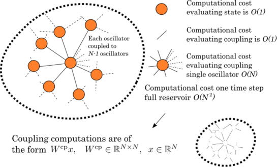
Figure 1: $N$-coupled STO simulations are suitable for parallelization for sufficiently large $N$ as the coupling computations are matrix multiplications.

In this paper we benchmark CPU and GPU implementations for simulating reservoirs given by $N$-coupled STOs. The GPU implementation is motivated by the fact that the coupling terms are of complexity $O(N^{2})$ which can run quickly on GPUs due to their high performing parallelization ability. Each implementation is optimal in some $N$ range. We show that the $N$ used in the literature is sufficiently large that GPUs are quicker than CPUs. The methods considered here are general and can be applied to any reservoir which can be approximated using an explicit method. This paper is accompanied by a github repository with the benchmarking code [Jon23].

2 Background

GPU-deployed reservoirs. In [GMP17, Sch18] a GPU-deployment of Echo State Network (ESN) is studied with a focus on stacking ESNs. However, no ablation studies are given of CPU versus GPU computations. In addition, ESNs are not described by differential equations and ESN do not have a physical representation.

ODE solving with GPUs. Neural networks have made impressive contribution to a new range of ODE solvers [CRBD18a, CRBD18b, GDY19, CGH⁺20]. Although their performance is incredible, these results typically lack rigorous statements concerning convergence and error estimates. As a consequence neural net approaches are not widely adopted by standard solvers, for example COMSOL, FreeFEM, Matlab, Mathematica, still rely on conventional methods that are deployed on CPUs. [Che18] contains some explicit solvers for GPU which would be more efficient than CPU if the system is sufficiently large and parallizable. In [BKAS23] a PyTorch based micromagnetic simulation library is presented. The repository contains code for simulating a single spin-torque oscillator. There is no direct way to introduce the coupling between the oscillators without tearing the code apart.

Reservoir computer parameters and number of nodes. In theoretical reservoir studies which focus on predicting complicated chaotic time series the coupled components are typically of order $O(10^{3})$ [JH04, GBGB21, PHG⁺18]. For a physical reservoir this is not within the realm of possibilities and one typically only tests 1 device [TTM⁺18, TRAA⁺17]. Generally, in a virtual setting improving reservoir computer performance and understanding the underlying dynamics requires an exploration of the parameter space [LHO18, FTA21, AYT⁺20, PLH⁺17]. As the reservoir computer has to be trained and tested for each parameter this is a computationally expensive task.

3 Methodology

3.1 Coupled STO equations

We consider $N$-coupled STOs. The differential equations corresponding to the magnetization of the $k$th-STO, $\mathbf{m}_{k}(t)=(m_{k}^{x}(t),m_{k}^{y}(t),m_{k}^{z}(t))^{\top}$, can be obtained through the Landau–Lifshitz–Gilbert (LLG) equations. In Cartesian co-ordinates we can express them as the following first order ODE:

$$\frac{d\mathbf{m}_{k}}{dt}=-\frac{\gamma}{1+\alpha^{2}}\mathbf{m}_{k}\times\mathbf{b}_{k}(\mathbf{m},\textbf{u})-\frac{\alpha\gamma}{1+\alpha^{2}}\mathbf{m}_{k}\times(\mathbf{m}_{k}\times\mathbf{b}_{k}(\mathbf{m},\textbf{u}))$$ (1)

where $\mathbf{b}_{k}(\mathbf{m},\textbf{u})=\mathbf{H}^{\rm total}_{k}(\mathbf{m},\textbf{u})+H_{s}(\mathbf{m}_{k})\mathbf{p}\times\mathbf{m}_{k}$ with ${H}_{s}(\mathbf{m}_{k})=\frac{\hbar\eta I}{2e(1+\lambda\mathbf{m}_{k}\cdot\mathbf{p})MV}$ and the total field $\mathbf{H}^{\rm total}_{k}$ given by the sum of the effective magnetic field, spin-transfer torque, coupling field, and input field, $\mathbf{H}^{\rm total}_{k}(\mathbf{m},\mathbf{u})=\mathbf{H}(\mathbf{m}_{k})+\mathbf{H}^{\rm cp}_{k}(\mathbf{m})+\mathbf{H}^{{\rm in}}_{k}(\mathbf{u})$ with

$$\mathbf{H}(\mathbf{m}_{k}) =[H_{\rm appl}+(H_{K}-4\pi M)m_{k}^{z}]\mathbf{e}_{z},$$

$$\mathbf{H}^{{\rm cp}}_{k}(\mathbf{m}) =A_{\rm cp}\sum_{i=1}^{N}w^{\rm cp}_{k,i}m_{k}^{x}\mathbf{e}_{x},$$ (2)

$$\mathbf{H}_{k}^{\rm in}(\mathbf{u}) =A_{\rm in}\sum_{i=1}^{N_{\rm in}}w^{\rm in}_{k,i}u_{i}\mathbf{e}_{x}.$$ (3)

The input signal $\textbf{u}(t)=(u_{1}(t),u_{2}(t),\ldots,u_{N_{\rm in}}(t))^{\top}$ is a discrete-point series. Let $W^{\rm cp}\in{\mathbb{R}}^{N\times N}$ denote the coupling matrix given by $(W^{\rm cp})_{k,i}=w^{\rm cp}_{k,i}$. There is no self-coupling, $(W^{\rm cp})_{k,k}=0$, and $(W^{\rm cp})_{k,i}$ with $k\neq i$ sampled from a uniform distribution on $[-1,1]$. The spectral radius of $W^{\rm cp}$ is set to 1. The components $w^{\rm in}_{k,i}$ are sampled from a uniform distribution on $[-1,1]$. A summary of parameters is given in Table 1. The parameters are chosen such that the solution exhibits oscillatory motion. These parameter values have been used in various reservoir experiments (virtual and physical) [KYF⁺13, TIT⁺17].

Symbol	Definition	Value
$\gamma$	gyromagnetic ratio	$1.764\cdot 10^{7}$ rad/Oe s
$\alpha$	Gilbert damping constant	0.005
$M$	saturation magnetization	1448.3 emu/cm3
$H_{\rm K}$	interfacial magnetic anisotropy field	18.616 kOe
$H_{\rm appl}$	applied field	200 Oe
$\eta$	spin polarization	0.537
$\lambda$	spin-transfer torque asymmetry	0.288
$I$	electric current	2.5mA
$V$	volume of free layer	$\pi\cdot 60^{2}\cdot 2$ nm3
$e$	elementary charge	$1.60217733\cdot 10^{-19}$ C
$\hbar$	Planck constant, reduced	$1.05457266\cdot 10^{-34}$ Js
$\mathbf{p}$	perturbed direction of pinned layer magnetization	$(1,0,6.123234\cdot 10^{-17})^{\top}$
$A_{\rm cp}$	coupling amplitude	1 Oe
$A_{\rm in}$	input amplitude	1 Oe

Table 1: Summary of parameters

We note that the state space is 3$N$-dimensional. Typically, $N$-states are used as the nodes of the reservoir. For initial conditions we consider

$$\mathbf{m}_{k}(0)=(\sin(\phi_{0})\cos(\phi_{0}),\sin(\phi_{0})\sin(\phi_{0}),\cos(\phi_{0}))^{\top},$$ (4)

with $\phi_{0}=2\pi/360$. Observe that $\mathbf{m}_{k}(0)\approx(0,0,1)^{\top}$ and that $|\mathbf{m}_{k}(0)|=1$. Straightforward calculation shows that $|\mathbf{m}_{k}|$ is conserved [BMS09]. Then, from (4) it follows that

$$|\mathbf{m}_{k}|=1.$$ (5)

Straightforward computations shows that evaluation of the vector field (1) is $O(N^{2})$. Numerically we can validate this by showing that the computation time of the vector field for random initialization increases quadratically in $N$, see Figure 2

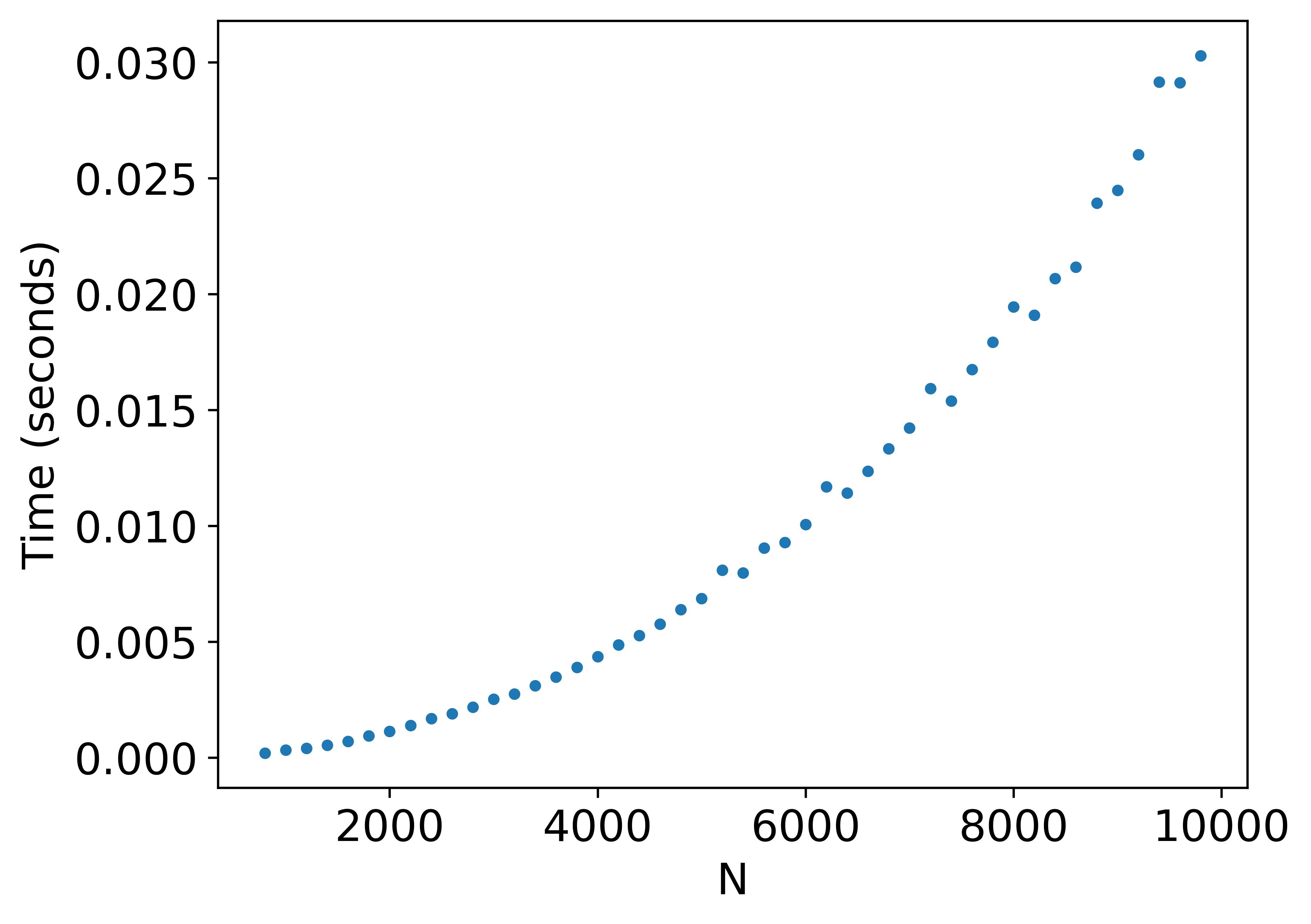
(a) Linear scale

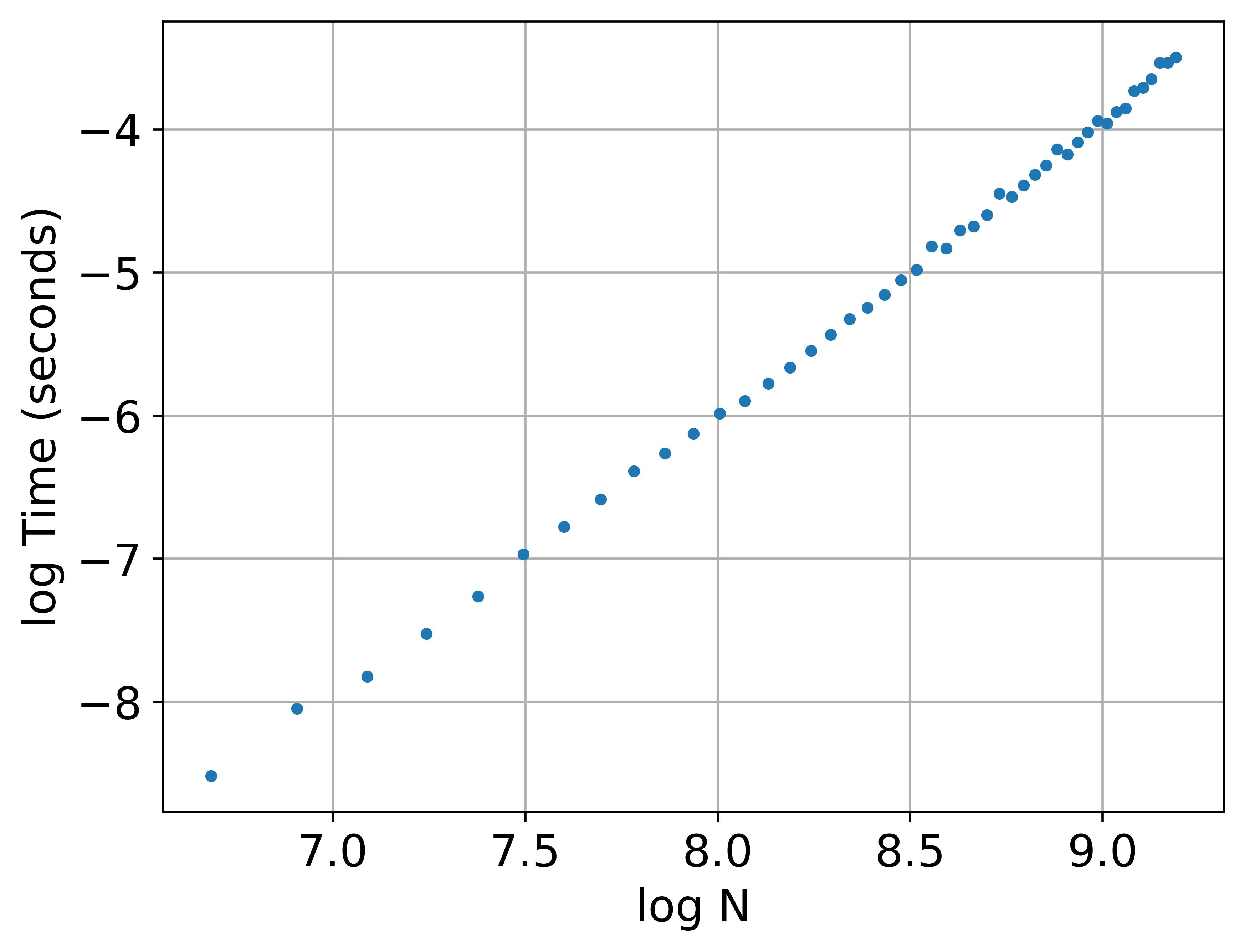
(b) Log scale

Figure 2: Computation time vector field for random initialization of $\mathbf{m}$

3.2 Benchmark test

For the benchmark test we set the input, $\mathbf{u}$, equal to zero as the input field term (3) is $O(1)$. We observe that the coupling field term (2) is $O(N)$. Observe that if the coupling field is set to 0 the vector field can be evaluated in $O(N)$. Hence, for meaningful results the coupling field has to be incorporated in the benchmark test. We fix the precision to float64.

Based on Section 2 we consider the $N$-range 1 to 10 000.

We solve Equation (1) using (classic) 4th order Runge–Kutta with step size $10^{-11}$ for $5\cdot 10^{5}$ steps. To validate the correctness for a given $N$ we check for each implementation whether the solutions and the conservation law $|\mathbf{m}_{i}|=1$ are identical.

3.3 CPU and GPU implementations

We consider the following Python implementations for the benchmark test:

• CPU, Numpy (Base): vectorized Numpy,

• CPU, Numba-vanilla: straightforward Numba [LPS15],

• CPU, Numba-parallel: parallelization with Numba,

• GPU, Torch: Pytorch tensor running on CUDA.

We provide additional details to the methods. Here we use community provided Numpy code as a baseline. Numba-vanilla is a fully sequential Numba implementation. When running Numba-vanilla we observed that the coupling field (2) is a bottle neck as $N$ increases. Hence, in Numba-parallel we optimize the coupling field computation by parallelization. Over the full vector field the coupling field can be written as a matrix calculation of the form $W^{cp}x$ with $x\in\mathbb{R}^{N}$. In Numba-parallel only the coupling field computation is parallelized. Finally, Numba acts as a JIT (Just-In-Time) compiler. We chose to compile the code prior to benchmarking.

We finally note that the order of performing operations differs for each implementation. This leads to a machine precision difference in the approximation of the solutions at the first time step. The differences between methods will grow as the number of steps are increased. However, this difference is at least a factor $10^{-6}$ smaller than the error corresponding to the preserved quantity $|\mathbf{m}_{i}|-1$. The repository [Jon23] contains supplemental experiments.

3.4 Hardware and module versions

The CPU and GPU used for these experiments are AMD Ryzen 9 5950X (16-core) and Nvidia RTX A4500, respectively.

We use Numpy v1.24, Numba v0.57, Torch v2.0. We note that Numpy v1.24 is the most recent Numba-compatible version.

4 Results

In Table 2 we present the computation times for the benchmark test for different $N$ and in Table 3 we present the factor improvement over the Numpy base which is an improvement over implementations used in the literature  [AKT⁺22]. We note that Table 2 concerns averaged results. However, deviations over multiple runs are small. For all computations the standard deviation is at least less than 2 orders of the leading decimal of the mean.

For small $N$ Numba-vanilla has the quickest computation times with a factor improvement of $O(10)$ over the base. For $N$ sufficiently large Numba-parallel performs better than the base with best computation times at $N=1000$ with respect to the other implementations. Finally, the performance boost through parallelization is most visible for the GPU which beats the CPU for $N\geq 2500$. The GPU hits a factor $O(10)$ improvement over the base as $N$ is increased.

		$N$
CPU/GPU	Method	1	10	100	1000	2500	5000	10000
CPU	Numpy (Base)	0.81s	0.93s	1.12s	5.78s	36.38s	2.79m	13.40m
CPU	Numba-vanilla	0.010s	0.016s	0.14s	12.56s	86.23s	5.99m	23.66m
CPU	Numba-parallel	X	0.48s	0.60s	2.27s	21.59s	2.60m	11.54m
GPU	Torch	X	7.47s	7.55s	7.14s	7.59s	0.22m	0.56m

Table 2: Computation time. Here s denotes seconds and m denotes minutes. For each $N$ the best computation time is denoted in bold.

Numba-vanilla does not have any in-built method to deal with large systems, contrary to Numpy. Hence, it only performs better than the Numpy base for small systems. For $N\geq 10^{3}$ the overhead of parallelization becomes cost-effective as Numba-parallel beats the other implementations. This argument also applies to the GPU results. For small matrix computations the GPU cannot function optimally which might be the cause for the non-increasing computation times occurring for $N\leq 10^{3}$.

		$N$
CPU/GPU	Method	1	10	100	1000	2500	5000	10000
CPU	Numba-vanilla	78.9	57.9	7.9	0.5	0.4	0.5	0.6
CPU	Numba-parallel	X	1.9	1.9	2.6	1.7	1.1	1.2
GPU	Torch	X	0.1	0.1	0.8	4.8	12.9	23.8

Table 3: Speed-factor with respect to base (Factor = time base / time method). For each $N$ the best factor is denoted in bold.

5 Conclusion and future work

In this work we present implementations for speeding up coupled STO simulations for reservoir computing. We obtain a speed factor improvement of at least 2.6 which goes up to $O(10)$ for $N\sim O(10)$ and $O(10^{4})$. However, the implementations for CPU and GPU considered in this paper apply to any reservoir whose evolution can be approximated using an explicit method. This paper is accompanied by a github respository containing the benchmarking code.

An important result is that GPU based reservoir computing should be considered when improving computation times. Overhead for GPU computations is high. Hence, a priori it is unclear if GPU usage is meaningful for differential equations. Our work shows by example that in a virtual setting the reservoir nodes are of an order that GPU implementations should be tested for performance.

By removing reservoir nodes and artificially replacing them using a delay-operation, such as multiplexing, the computational time can be reduced. However, this does not necessarily increase the information processing capabilities of the reservoir. Hence, it is preferable to develop numerical methods that speed up the simulation of natural reservoirs. This work contributes to this direction.

The physical implementation of reservoirs with a large number of interacting components is likely not a topic that can be studied in the near future. However, by considering a spatial and discretized system, i.e. moving from ODEs to PDEs, we can efficiently construct high dimensional reservoirs. A fluid is a suitable candidate for this approach. Pioneering work was accomplished in [GNN21] by achieving the first vortex (virtual) reservoir computer. The underlying CPU-based computations are computationally intensive (order of days) and would greatly benefit from a GPU-based approach.

References

- [AKT+22] N. Akashi, Y. Kuniyoshi, S. Tsunegi, T. Taniguchi, M. Nishida, R. Sakurai, Y. Wakao, K. Kawashima, and K. Nakajima. A coupled spintronics neuromorphic approach for high-performance reservoir computing. Adv. Intell. Syst., 4:2200123, 2022.
- [AYT+20] N. Akashi, N. Yamaguchi, S. Tsunegi, T. Taniguchi, M. Nishida, R. Sakurai, Y. Wakao, and K. Nakajima. Input-driven bifurcations and information processing capacity in spintronics reservoirs. Phys. Rev. Research, 2:043303, 2020.
- [BKAS23] F. Bruckner, S. Koraltran, C. Abert, and D. Suess. magnum.np: a pytorch based gpu enhanced finite difference micromagnetic simulation framework for high level development and inverse design. Scientific Reports, 13(12054), 2023.
- [BMS09] G. Bertotti, I.D. Mayergoyz, and C. Serpico. Nonlinear magnetization Dynamics in Nanosystems. Elsevier, Oxford, 2009.
- [CGH+20] M. Cranmer, S. Greydanus, S. Hoyer, P. Battaglia, D. Spergel, and S. Ho. Lagrangian neural networks. arXiv preprint arXiv:2003.04630, 2020.
- [Che18] R.T.Q. Chen. torchdiffeq. https://github.com/rtqichen/torchdiffeq, 2018.
- [CRBD18a] R.T.Q. Chen, Y. Rubanova, J. Bettencourt, and D. Duvenaud. Neural ordinary differential equations. Advances in Neural Information Processing Systems, 2018.
- [CRBD18b] R.T.Q. Chen, Y. Rubanova, J. Bettencourt, and D.K. Duvenaud. Neural ordinary differential equations. Advances in neural information processing systems, 31, 2018.
- [DVSM12] J. Dambre, D. Verstraeten, B. Schrauwen, and S. Massar. Information processing capacity of dynamical systems. Sci. Rep., 2:514, 2012.
- [FFN+18] T. Furuta, K. Fujii, K. Nakajima, S. Tsunegi, H. Kubota, Y. Suzuki, and S. Miwa. Macromagnetic simulation for reservoir computing utilizing spin dynamics in magnetic tunnel junctions. Physical Review Applied, 10(3):034063, 2018.
- [FTA21] A. Flynn, V.A. Tsachouridis, and A. Amann. Multifunctionality in a reservoir computer. Chaos: An Interdisciplinary Journal of Nonlinear Science, 31(1), 2021.
- [GBGB21] D.J. Gauthier, E. Bollt, A. Griffith, and W.A.S. Barbosa. Next generation reservoir computing. Nature communications, 12(1):5564, 2021.
- [GDY19] S. Greydanus, M. Dzamba, and J. Yosinski. Hamiltonian neural networks. Advances in neural information processing systems, 32, 2019.
- [GMP17] C. Gallicchio, A. Micheli, and L. Pedrelli. Deep reservoir computing: A critical experimental analysis. Neurocomputing, 268:87–99, 2017.
- [GNN21] K. Goto, K. Nakajima, and H. Notsu. Twin vortex computer in fluid flow. New Journal of Physics, 23(6):063051, 2021.
- [GP10] S. Gerardin and A. Paccagnella. Present and future non-volatile memories for space. IEEE Transactions on Nuclear Science, 57(6):3016–3039, 2010.
- [GQC+20] J. Grollier, D. Querlioz, K. Camsari, K.Y.and Everschor-Sitte, S. Fukami, and M.D. Stiles. Neuromorphic spintronics. Nat. Electron., 3:360–370, 2020.
- [JCZ+19] W. Jiang, L. Chen, K. Zhou, L. Li, Q. Fu, Y. Du, and R.H. Liu. Physical reservoir computing using magnetic skyrmion memristor and spin torque nano-oscillator. Appl. Phys. Lett., 115:192403, 2019.
- [JH04] H. Jaeger and H. Haas. Harnessing Nonlinearity: Predicting Chaotic Systems and Saving Energy in Wireless Communication. Science, 304:78, 2004.
- [Jon23] T.G. de Jong. Reservoir acceleration: High-speed reservoir computing. https://github.com/mathowl/reservoir_acceleration, 2023.
- [KK17] T.M. Kiwamu Kudo. Self-feedback electrically coupled spin-hall oscillator array for pattern-matching operation. Applied Physics Express, 10(4):043001, mar 2017.
- [KKT+21] A. Kamimaki, T. Kubota, S. Tsunegi, K. Nakajima, T. Taniguchi, J. Grollier, V. Cros, K. Yakushiji, A. Fukushima, S. Yuasa, and H. Kubota. Chaos in spin-torque oscillator with feedback circuit. Phys. Rev. Research, 3:04216, 2021.
- [KSM+19] T. Kanao, H. Suto, K. Mizushima, H. Goto, T. Tanamoto, and T. Nagasawa. Reservoir Computing on Spin-Torque Oscillator Array. Phys. Rev. Applied, 12:024052, 2019.
- [KTN21] T. Kubota, H. Takahashi, and K. Nakajima. Unifying framework for information processing in stochastically driven dynamical systems. Phys. Rev. Research, 3:043135, 2021.
- [KYF+13] H. Kubota, K. Yakushiji, A. Fukushima, S. Tamaru, M. Konoto, T. Nozaki, S. Ishibashi, T. Saruya, S. Yuasa, T. Taniguchi, et al. Spin-torque oscillator based on magnetic tunnel junction with a perpendicularly magnetized free layer and in-plane magnetized polarizer. Applied Physics Express, 6(10):103003, 2013.
- [LHO18] Z. Lu, B.R. Hunt, and E. Ott. Attractor reconstruction by machine learning. Chaos: An Interdisciplinary Journal of Nonlinear Science, 28(6), 2018.
- [LPS15] S.K. Lam, A. Pitrou, and S. Seibert. Numba: A llvm-based python jit compiler. In Proceedings of the Second Workshop on the LLVM Compiler Infrastructure in HPC, pages 1–6, 2015.
- [MLR+19] D. Marković, N. Leroux, M. Riou, F. Abreu Araujo, J. Torrejon, D. Querlioz, A. Fukushima, S. Yuasa, J. Trastoy, P. Bortolotti, et al. Reservoir computing with the frequency, phase, and amplitude of spin-torque nano-oscillators. Applied Physics Letters, 114(1):012409, 2019.
- [Nak20] K. Nakajima. Physical reservoir computing - an introductory perspective. Jpn. J. Appl. Phys., 59:060501, 2020.
- [PHG+18] J. Pathak, B. Hunt, M. Girvan, Z. Lu, and E. Ott. Model-free prediction of large spatiotemporally chaotic systems from data: A reservoir computing approach. Physical review letters, 120(2):024102, 2018.
- [PLH+17] J. Pathak, Z. Lu, B.R. Hunt, M. Girvan, and E. Ott. Using machine learning to replicate chaotic attractors and calculate lyapunov exponents from data. Chaos: An Interdisciplinary Journal of Nonlinear Science, 27(12), 2017.
- [PW96] F.W. Patten and S.A. Wolf. Overview of the darpa non-volatile magnetic memory program. In Proceedings of Nonvolatile Memory Technology Conference, pages 1–2, 1996.
- [RTT+18] M. Romera, P. Talatchian, S. Tsunegi, F. Abreu Araujo, V. Cros, P. Bortolotti, J. Trastoy, K. Yakushiji, A. Fukushima, H. Kubota, et al. Vowel recognition with four coupled spin-torque nano-oscillators. Nature, 563(7730):230–234, 2018.
- [Sch18] N. Schaetti. Echotorch: Reservoir computing with pytorch. https://github.com/nschaetti/EchoTorch, 2018.
- [SGM19] E. Strubell, A. Ganesh, and A. McCallum. Energy and policy considerations for deep learning in NLP. CoRR, abs/1906.02243, 2019.
- [TAN+19] T. Taniguchi, N. Akashi, H. Notsu, M. Kimura, H. Tsukahara, and K. Nakajima. Chaos in nanomagnet via feedback current. Phys. Rev. B, 100:174425, 2019.
- [TGLM20] N.C. Thompson, K. Greenewald, K. Lee, and G.F. Manso. The computational limits of deep learning. arXiv preprint arXiv:2007.05558, 2020.
- [TIT+17] T. Taniguchi, T. Ito, S. Tsunegi, H. Kubota, and Y. Utsumi. Relaxation time and critical slowing down of a spin-torque oscillator. Physical Review B, 96(2):024406, 2017.
- [TKK+23] S. Tsunegi, T. Kubota, A. Kamimaki, J. Grollier, V. Cros, K. Yakushiji, A. Fukushima, S. Yuasa, H. Kubota, K. Nakajima, and T. Taniguchi. Information processing capacity of spintronic oscillator. Advanced Intelligent Systems, 5(9):2300175, 2023.
- [TRAA+17] J. Torrejon, M. Riou, F. Abreu Araujo, S. Tsunegi, G. Khalsa, D. Querlioz, P. Bortolotti, V. Cros, K. Yakushiji, A. Fukushima, H. Kubota, S. Yuasa, M.D. Stiles, and J. Grollier. Neuromorphic computing with nanoscale spintronic oscillators. Nature, 547:428, 2017.
- [TTM+18] S. Tsunegi, T. Taniguchi, S. Miwa, K. Nakajima, K. Yakusjiji, A. Fukushima, S. Yuasa, and H. Kubota. Evaluation of memory capacity of spin torque oscillator for recurrent neural networks. Jpn. J. Appl. Phys., 57:120307, 2018.
- [TTN+19] S. Tsunegi, T. Taniguchi, K. Nakajima, S. Miwa, K. Yakusjiji, A. Fukushima, S. Yuasa, and H. Kubota. Physical reservoir computing based on spin torque oscillator with forced synchronization. Appl. Phys. Lett., 114:164101, 2019.
- [WAR+19] J. Williame, A.D. Accoily, D. Rontani, M. Sciamanna, and J.V. Kim. Chaotic dynamics in a macrospin spin-torque nano-oscillator with delayed feedback. Appl. Phys. Lett., 114:232405, 2019.
- [YAN+19] T. Yamaguchi, N. Akashi, K. Nakajima, S. Tsunegi, H. Kubota, and T. Taniguchi. Synchronization and chaos in a spin-torque oscillator with a perpendicularly magnetized free layer. Phys. Rev. B, 100:224422, 2019.
- [YAT+20] T. Yamaguchi, N. Akashi, S. Tsunegi, H. Kubota, K. Nakajima, and T. Taniguchi. Periodic structure of memory function in spintronics reservoir with feedback current. Phys. Rev. Research, 2:023389, 2020.
- [YZL07] Z. Yang, S. Zhang, and Y.C. Li. Chaotic Dynamics of Spin-Valve Oscillators. Phys. Rev. Lett., 99:134101, 2007.