Simple and general unitarity conserving numerical real time propagators of time dependent Schrödinger equation based on Magnus expansion

Abstract

Magnus expansion (ME) provides a general way to expand the real time propagator of a time dependent Hamiltonian within the exponential such that the unitarity is satisfied at any order. We use this property and explicit integration of Lagrange interpolation formulas for the time dependent Hamiltonian within each time interval and derive approximations that preserve unitarity for the differential time evolution operators of general time dependent Hamiltonians. The resulting second order approximation is the same as using the average of Hamiltonians for two end points of time. We identify three fourth order approximations involving commutators of Hamiltonians at different times, and also derive a sixth order expression. Test of these approximations along with other available expressions for a two state time dependent Hamiltonian with sinusoidal time dependences provide information on relative performance of these approximations, and suggest that the derived expressions can serve as useful numerical tools for time evolution for time resolved spectroscopy, quantum control, quantum sensing, and open system quantum dynamics.

I Introduction

Accurate numerical integration of time dependent Schrödinger equation is crucial for reliable modeling of time resolved spectroscopy,[1, 2, 3, 4] quantum control,[5, 6, 7] and more recently quantum sensing.[8] Even for open system quantum dynamics studies employing quantum master equations,[9, 10, 11, 12, 13, 4, 14, 15] it becomes a necessary step if the equation is solved in the interaction picture[9, 10, 11, 12, 13] with respect to a time dependent system Hamiltonian. Thus, developing an accurate and efficient general numerical approximation for the real time propagator of a time dependent Hamiltonian has broad implications and applications. One key property that needs to be ensured for such approximation is the conservation of unitarity. If this is not satisfied, unphysical behavior including violation of norm conservation is expected to arise. Methods based on Trotter[16, 17] and Suzuki factorizations[18, 19] or their generalizations[20, 21] have played important roles in this respect, but their extension to time dependent Hamiltonian remain difficult in general although some progress was made.[22] Time ordered exponential operator serves as a general formal solution, but its simple perturbative truncation is not guaranteed to preserve unitarity. Magnus expansion (ME)[23, 24, 25] serves as a superior starting point in this respect because it is designed to preserve unitarity at any finite order of series and is applicable to any time dependent Hamiltonian.

In a sense, ME can be viewed as a specific expansion of the time ordered exponential operator. Then, each term of the Magnus expansion can be considered as a partial re-summation of simple perturbative terms of certain class up to an infinite order. Indeed, during past couple of decades, significant progress[25] has been made clarifying this view of ME. A well-defined mathematical criterion for the existence of ME now exists[25, 26] and exact formal expressions up to an infinite order based on the graph theory have been derived. Most recently, ME was studied using the theory of graded Lie algebra [27] and Taylor expansions.[28] These advances serve as solid basis for employing ME as a practical tool for general quantum dynamics, and have also produced practical algorithms for numerical time evolution.

In this paper, we show that combination of Lagrange interpolating polynomials and ME leads to simple and general expressions for finite order MEs for differential propagators, which then can be used for numerical time evolution for a general time dependent Hamiltonian. We provide detailed derivation of these expressions and also summarize others available,[26, 29] which are then tested for a simple two state time dependent Hamiltonian. The paper concludes with a summary of major implication and applications of this work.

II Magnus expansion up to the fourth order and approximate propagators

II.1 Expressions of ME

Consider a time evolution operator $U(t)$ that satisfies the following time dependent Schrödinger equation:

$$\frac{\partial}{\partial t}U(t)=-\frac{i}{\hbar}H(t)U(t),$$ (1)

where $H(t)$ is an arbitrary time dependent Hamiltonian. We are interested in finding an explicit expression for the time evolution operator for $t\in[t_{k},t_{k+1}]$ with $t_{k+1}-t_{k}=\delta t$, which is denoted as $U_{\delta}(t_{k+1},t_{k})$, such that

$$U(t_{k+1})=U_{\delta t}(t_{k+1},t_{k})U(t_{k}).$$ (2)

Application of ME[23, 25] to $U_{\delta t}(t_{k+1},t_{k})$ leads to the following formal expression:

$$U_{\delta t}(t_{k+1},t_{k})=\exp\left\{\sum_{n=1}^{\infty}\frac{1}{n!}\left(-\frac{i}{\hbar}\right)^{n}M_{n}(t_{k+1},t_{k})\right\},$$ (3)

where $M_{n}(t_{k+1},t_{k})$ up to the fourth order are well known[24, 25, 30] and can be expressed as follows:

$$M_{1}(t_{k+1},t_{k}) = \int_{t_{k}}^{t_{k+1}}d\tau H(\tau),$$ (4)

$$M_{2}(t_{k+1},t_{k}) = \int_{t_{k}}^{t_{k+1}}d\tau\int_{t_{k}}^{\tau}d\tau^{\prime}[H(\tau),H(\tau^{\prime})],\hskip 21.68121pt$$ (5)

$$M_{3}(t_{k+1},t_{k}) = \int_{t_{k}}^{t_{k+1}}d\tau\int_{t_{k}}^{\tau}d\tau^{\prime}\int_{t_{k}}^{\tau^{\prime}}d\tau^{\prime\prime}$$ (6)

$$\hskip 36.135pt\Big{(}\left[H(\tau),[H(\tau^{\prime}),H(\tau^{\prime\prime})]\right]$$

$$\hskip 36.135pt+\left[[H(\tau),H(\tau^{\prime})],H(\tau^{\prime\prime})\right]\Big{)},$$

$$M_{4}(t_{k+1},t_{k}) = 2\int_{t_{k}}^{t_{k+1}}d\tau\int_{t_{k}}^{\tau}d\tau^{\prime}\int_{t_{k}}^{\tau^{\prime}}d\tau^{\prime\prime}\int_{t_{k}}^{\tau^{\prime\prime}}d\tau^{\prime\prime\prime}$$ (7)

$$\Big{(}[[[H(\tau),H(\tau^{\prime})],H(\tau^{\prime\prime})],H(\tau^{\prime\prime\prime})]$$

$$+[H(\tau),[[H(\tau^{\prime}),H(\tau^{\prime\prime})],H(\tau^{\prime\prime\prime})]]$$

$$+[H(\tau),[H(\tau^{\prime}),[H(\tau^{\prime\prime}),H(\tau^{\prime\prime\prime})]]]$$

$$+[H(\tau^{\prime}),[H(\tau^{\prime\prime}),[H(\tau^{\prime\prime\prime}),H(\tau)]]]\Big{)}.$$

As is clear from the above expressions up to the fourth order, the $n$th order ME term consists of $n$ ordered time integrations. Thus, unless the time dependent Hamiltonian has singularity, considering up to the $n$th term of ME will ensure that the numerical algorithm is exact up to $\delta t^{n}$ at the minimum. In practice, actual order is even better because an $n$th term involves $n-1$ nested commutators. In addition, terms of even order of $\delta t$ in general disappear once explicit expansion is made with respect to $\delta t$ in a symmetric manner, as shown in Appendix A, which renders the practical order of accuracy of any nominally odd order approximation to become the next order. More detailed consideration of this is provided below.

II.2 Approximations based on polynomial approximations

We here consider the cases where the time dependent Hamiltonian is smooth enough to allow polynomial expansions within each interval $[t_{k},t_{k+1}]$. More specifically, we assume that $H(t)$ can be approximated as

$$H(t)=H^{(l)}(t)+O(\delta t^{l+1}),$$ (8)

where explicit expressions for $H^{(l)}$ for $l=0,\cdots,3$ are shown below

$$H^{(0)}(t) = \frac{1}{2}(H_{k}+H_{k+1}),$$ (9)

$$H^{(1)}(t) = H_{k}\frac{(t_{k+1}-t)}{\delta t}+H_{k+1}\frac{(t-t_{k})}{\delta t},\hskip 28.90755pt$$ (10)

$$H^{(2)}(t) = 2H_{k}\frac{(t_{k+1}-t)(t_{k+\frac{1}{2}}-t)}{\delta t^{2}}$$ (11)

$$+ 4H_{k+\frac{1}{2}}\frac{(t_{k+1}-t)(t-t_{k})}{\delta t^{2}}$$

$$+ 2H_{k+1}\frac{(t-t_{k+\frac{1}{2}})(t-t_{k})}{\delta t^{2}},\hskip 50.58878pt$$

$$H^{(3)}(t) = \frac{9}{2}H_{k}\frac{(t_{k+1}-t)(t_{k+\frac{2}{3}}-t)(t_{k+\frac{1}{3}}-t)}{\delta t^{3}}$$ (12)

$$+ \frac{27}{2}H_{k+\frac{1}{3}}\frac{(t_{k+1}-t)(t_{k+\frac{2}{3}}-t)(t-t_{k})}{\delta t^{3}}$$

$$+ \frac{27}{2}H_{k+\frac{2}{3}}\frac{(t_{k+1}-t)(t-t_{k+\frac{1}{3}})(t-t_{k})}{\delta t^{3}}$$

$$+ \frac{9}{2}H_{k+1}\frac{(t-t_{k+\frac{2}{3}})(t-t_{k+\frac{1}{3}})(t-t_{k})}{\delta t^{3}}.$$

In above expressions, $H_{k}$ is a short notation for $H(t_{k})$. We combine the above expressions with MEs of different order and obtain approximations for $U_{\delta t}(t_{k+1},t_{k})$ of different order. To this end, we introduce a short notation $M_{n}^{(l)}$ defined as follows:

$$M^{(l)}_{n} \equiv M_{n}(t_{k+1},t_{k})\mbox{ that uses }H^{(l)}(t)$$

$$\mbox{ instead of }H(t)\mbox{ in the integrands}$$

II.2.1 Second order propagator

Let us first start with the simplest second order propagator $U_{\delta t}^{(2)}(t_{k+1},t_{k})$ such that

$$U_{\delta t}(t_{k+1},t_{k})=U_{\delta t}^{(2)}(t_{k+1},t_{k})+O(\delta t^{3})$$ (13)

To this end, consideration up to the second order ME is sufficient. Since each integration over the interval of $\delta t$ increases the order of $\delta t$, we find that the corresponding second order approximation is sufficient.

$$U_{\delta t}^{(2)}(t_{k+1},t_{k})=\exp\left\{-\frac{i}{\hbar}M_{1}^{(1)}-\frac{1}{2\hbar^{2}}M_{2}^{(0)}\right\}.$$ (14)

In the above expression, it is easy to find that

$$M_{1}^{(1)}=\int_{t_{k}}^{t_{k+1}}d\tau H^{(1)}(\tau)=\frac{\delta t}{2}\left(H_{k}+H_{k+1}\right).$$ (15)

On the other hand, $M_{2}^{(0)}=0$ since $[H^{(0)}(t),H^{(0)}(t)]=0$. Therefore,

$$U_{\delta t}^{(2)}(t_{k+1},t_{k})=\exp\left\{-\frac{i\delta t}{2\hbar}(H_{k}+H_{k+1})\right\}.$$ (16)

Thus, the second order approximation for the differential propagator based on ME is the same as the usual symmetric average approximation within the exponent for each propagator.

II.2.2 Third order propagator

The third order propagator $U_{\delta t}^{(3)}(t_{k},t_{k+1})$ is nominally accurate up to the order of $\delta t^{3}$ as follows:

$$U_{\delta t}(t_{k+1},t_{k})=U_{\delta t}^{(3)}(t_{k+1},t_{k})+O(\delta t^{4}).$$ (17)

However, in practice, as shown in Appendix A, $U_{\delta t}^{(3)}(t_{k+1},t_{k})$ is in general exact up to the order of $\delta t^{4}$ since there are no terms of even order with respect to $\delta t$ once all the coefficients are expressed in a symmetrical manner. Following the same reasoning as in the second order approximation and noting that $M_{3}^{(0)}=0$, we find that

$$U_{\delta t}^{(3)}(t_{k+1},t_{k})=\exp\left\{-\frac{i}{\hbar}M_{1}^{(2)}-\frac{1}{2\hbar^{2}}M_{2}^{(1)}\right\}.$$ (18)

Each of the two terms in the above expression can be calculated easily, as described in Appendix B, and can be expressed as

$$M_{1}^{(2)}=\frac{\delta t}{6}(H_{k}+4H_{k+\frac{1}{2}}+H_{k+1}),$$ (19)

$$M_{2}^{(1)}=\frac{\delta t^{2}}{6}[H_{k+1},H_{k}].$$ (20)

In the above expression, it is important to note that $M_{1}^{(2)}$ is in fact exact up to the order of $\delta t^{4}$, which can be proven directly by integration of any cubic function of $t$. This is because of the cancellation of the cubic term around the quadratic polynomial approximation. Thus, $M_{1}^{(2)}$ can still be used for the fourth order propagator considered in the next subsection.

II.2.3 Fourth order propagator

The fourth order propagator $U_{\delta t}^{(4)}(t_{k+1},t_{k})$ is accurate up to the order of $\delta t^{4}$ as follows:

$$U_{\delta t}(t_{k+1},t_{k})=U_{\delta t}^{(4)}(t_{k+1},t_{k})+O(\delta t^{5}).$$ (21)

Following the same reasoning as in the second and third order approximations and noting that $M_{4}^{(0)}=0$, we find that

$$U_{\delta t}^{(4)}(t_{k+1},t_{k})=\exp\left\{-\frac{i}{\hbar}M_{1}^{(2)}-\frac{1}{2\hbar^{2}}M_{2}^{(2)}+\frac{i}{6\hbar^{3}}M_{3}^{(1)}\right\},$$

(22)

where $M_{1}^{(2)}$ is given by Eq. (19) and was used since this is exact up to the order of $\delta t^{4}$. $M_{2}^{(2)}$ and $M_{3}^{(1)}$ are expressed as

$$M_{2}^{(2)}=\frac{\delta t^{2}}{30}\left([H_{k+1},H_{k}]+4[H_{k+\frac{1}{2}},H_{k}]+4[H_{k+1},H_{k+\frac{1}{2}}]\right),$$

$$\hskip 25.29494pt=\frac{\delta t^{2}}{30}[H_{k}+4H_{k+\frac{1}{2}},H_{k}-H_{k+1}],$$ (23)

$$M_{3}^{(1)}=\frac{\delta t^{3}}{40}[H_{k+1}-H_{k},[H_{k+1},H_{k}]].$$ (24)

Detailed derivations of the above expressions are provided in Appendix B. The second expression for $M_{2}^{(2)}$ in Eq. (23) is computationally a little more convenient, whereas the first expression makes it clear that $M_{2}^{(2)}$ is an odd function of $\delta t$.

Close inspection of Eq. (24) shows that the actual leading order term of $M_{3}^{(1)}$ is $O(\delta t^{5})$ within the polynomial approximation because $H_{k+1}-H_{k}=O(\delta t)$. Therefore, the following approximation is also exact up to the fourth order of $\delta t$:

$$U_{\delta t}^{(4)}(t_{k+1},t_{k})\approx\exp\left\{-\frac{i}{\hbar}M_{1}^{(2)}-\frac{1}{2\hbar^{2}}M_{2}^{(2)}\right\}.$$ (25)

Thus, overall, we find that the three approximations, Eqs. (18), (22), and (25), are all practically exact up to $\delta t^{4}$. Actual performance of these expressions will be tested through model calculations provided in the next section.

II.2.4 Fifth order propagator

The fifth order propagator $U_{\delta t}^{(5)}(t_{k},t_{k+1})$ is nominally accurate up to the order of $\delta t^{5}$ as follows:

$$U_{\delta t}(t_{k+1},t_{k})=U_{\delta t}^{(5)}(t_{k+1},t_{k})+O(\delta t^{6}).$$ (26)

However, this is practically exact up to the order of $\delta t^{6}$ since there are no even order terms of ME when expanded with respect to $\delta t$ as shown in Appendix A.

Following the same reasoning as in the second and third order approximations and noting that $M_{5}^{(0)}=0$, we find that

$$U_{\delta t}^{(5)}(t_{k+1},t_{k}) = \exp\left\{-\frac{i}{\hbar}M_{1}^{(4)}-\frac{1}{2\hbar^{2}}M_{2}^{(3)}+\frac{i}{6\hbar^{3}}M_{3}^{(2)}\right.$$ (27)

$$\left.\hskip 36.135pt+\frac{1}{24\hbar^{3}}M_{4}^{(1)}\right\},$$

where calculation of each term is straightforward. Final expressions of the first three terms are as follows:

$$M_{1}^{(4)}=\frac{\delta t}{90}\left(7H_{k}+32H_{k+\frac{1}{4}}+12H_{k+\frac{1}{2}}\right.\hskip 50.58878pt$$

$$\hskip 50.58878pt\left.+32H_{k+\frac{3}{4}}+7H_{k+1}\right),$$ (28)

$$M_{2}^{(3)}=\frac{\delta t^{2}}{3360}\left(117([H_{k+\frac{1}{3}},H_{k}]+[H_{k+1},H_{k+\frac{2}{3}}])\right.$$

$$\hskip 36.135pt+47[H_{k+1},H_{k}]+144([H_{k+1},H_{k+\frac{1}{3}}]+[H_{k+\frac{1}{3}},H_{k}])$$

$$\hskip 36.135pt\left.+729[H_{k+\frac{2}{3}},H_{k+\frac{1}{3}}]\right)$$

$$\hskip 28.90755pt=\frac{\delta t^{2}}{3360}\left[\frac{232}{39}H_{k}+\frac{1152}{13}H_{k+\frac{1}{3}}+72H_{k+\frac{2}{3}},\right.$$

$$\hskip 57.81621pt\left.2H_{k}+\frac{81}{8}H_{k+\frac{1}{3}}-\frac{13}{8}H_{k+1}\right]$$

$$\hskip 36.135pt+\frac{\delta t^{2}}{90}[H_{k+1},H_{k}],$$ (29)

$$M_{3}^{(2)}=\frac{\delta t^{3}}{2520}\Big{(}64[H_{k+\frac{1}{2}}+H_{k+1},[H_{k+\frac{1}{2}},H_{k}]]$$

$$\hskip 36.135pt+64[H_{k+\frac{1}{2}}+H_{k},[H_{k+\frac{1}{2}},H_{k+1}]]$$

$$\hskip 36.135pt+44\left([H_{k},[H_{k},H_{k+\frac{1}{2}}]]+[H_{k+1},[H_{k+1},H_{k+\frac{1}{2}}]]\right)$$

$$\hskip 36.135pt+9[H_{k+1}-H_{k},[H_{k+1},H_{k}]]\Big{)}.$$ (30)

The final term, $M_{4}^{(1)}$ in Eq. (25) becomes even more complicated, but we found that it can be simplified as follows:

$$M_{4}^{(1)}=\frac{\delta t^{4}}{210}[\frac{1}{c}H_{k}-H_{k+1},[H_{k+1}-cH_{k},[H_{k+1},H_{k}]]],$$ (31)

where $c=-\frac{5-\sqrt{21}}{2}$. More detailed explanation and its verification using a computer algebra system known as SymPy[31] are provided in Appendix C.

II.3 Other approximate expressions

There are other well established approximations[26, 29] for the differential propagator based on ME, for which we introduce $M(t_{k+1},t_{k})$ such that

$$U_{\delta t}(t_{k+1},t_{k})=\exp\left\{-\frac{i}{\hbar}M(t_{k+1},t_{k})\right\}.$$ (32)

Thus,

$$M(t_{k+1},t_{k})=\sum_{n=1}^{\infty}\frac{1}{n!}\left(-\frac{i}{\hbar}\right)^{n-1}M_{n}(t_{k+1},t_{k}).$$ (33)

Then, the three algorithms we consider in our notation can be summarized as follows:

1. 4th order expression using equally spaced points [Blanes 4th-order]:[26] This was derived based on reproducing the Taylor series of $M(t_{k+1},t_{k})$ in terms of univariate integrals, and is expressed in our notation as follows:

   $$M(t_{k+1},t_{k})=\frac{1}{6}\delta t(H_{k}+4H_{k+\frac{1}{2}}+H_{k+1})$$

   $$-\frac{i}{\hbar}\frac{\delta t^{2}}{72}[H_{k+1}-H_{k},H_{k}+4H_{k+\frac{1}{2}}+H_{k+1}].$$ (34)

   Note that this is similar but different from one of our 4th order approximations, Eq. (25).

2. 4th order expression using Gauss-Legendre points [Blanes-4th order (gauss)]:[26] This expression was derived using the same univariate integrals as above, but Gauss-Legendre points were used for the integral. For this, let us define

   $$\gamma_{1}=\frac{1}{2}-\frac{1}{6}\sqrt{3},$$ (35)

   $$\gamma_{2}=\frac{1}{2}+\frac{1}{6}\sqrt{3}.$$ (36)

   Then, employing $H_{k+\gamma_{1}}=H(t_{k}+\gamma_{1}\delta t)$ and $H_{k+\gamma_{2}}=H(t_{k}+\gamma_{2}\delta t)$, this can be expressed as follows:

   $$M(t_{k+1},t_{k}) = \frac{1}{2}\delta t(H_{k+\gamma_{1}}+H_{k+\gamma_{2}})$$ (37)

   $$- \frac{i}{\hbar}\frac{\sqrt{3}}{12}\delta t^{2}[H_{k+\gamma_{2}},H_{k+\gamma_{1}}].$$

   The above expression can also be obtained using the linear approximation for $M_{1}$ and $M_{2}$ in our expressions through the Gauss-Legendre points.

3. 4th order expression using Gauss-Legendre points (with additional 2nd order commutator) [Iserles 4th-order (gauss)]:[29] This was derived from binary trees by collecting all fourth-order terms and then making polynomial approximation between two points $t_{k}k+\gamma_{1}\delta t$ and $t_{k}+\gamma_{2}\delta t$. The resulting expression is

   $$M(t_{k+1},t_{k})=\frac{1}{2}\delta t(H_{k+\gamma_{1}}+H_{k+\gamma_{2}})$$

   $$-\frac{i}{\hbar}\frac{\sqrt{3}}{12}\delta t^{2}[H_{k+\gamma_{2}},H_{k+\gamma_{1}}]$$

   $$-\frac{1}{\hbar^{2}}\frac{1}{80}\delta t^{3}[H_{k+\gamma_{2}}-H_{k+\gamma_{1}},[H_{k+\gamma_{2}},H_{k+\gamma_{1}}]].$$ (38)

4. 6th order expressions using Gauss-Legendre points [Blanes 6th order (gauss)]:[26] This expression involves evaluation of the Hamiltonian at midpoint $t_{k+\frac{1}{2}}$ and two additional intermediate points. For this let us define

   $$\alpha_{1}=\frac{1}{2}-\frac{\sqrt{3}}{2\sqrt{5}},$$ (39)

   $$\alpha_{2}=\frac{1}{2}+\frac{\sqrt{3}}{2\sqrt{5}},$$ (40)

   and define $H_{k+\alpha_{1}}=H(t_{k}+\alpha_{1}\delta t)$ and $H_{k+\alpha_{2}}=H(t_{k}+\alpha_{2}\delta t)$. Then, the expression involves first calculating the following operators:

   $$B_{0}=\frac{5}{18}(H_{k+\alpha_{1}}+H_{k+\alpha_{2}})+\frac{4}{9}H_{k+\frac{1}{2}}$$ (41)

   $$B_{1}=\frac{\sqrt{15}}{36}\left(H_{k+\alpha_{2}}-H_{k+\alpha_{1}}\right)$$ (42)

   $$B_{2}=\frac{1}{24}\left(H_{k+\alpha_{1}}+H_{k+\alpha_{2}}\right)$$ (43)

   The above expressions are then used to calculate the following operators:

   $$M_{1}=\delta tB_{0},$$ (44)

   $$M_{2}=\delta t^{2}[B_{1},3B_{0}-12B_{2}],$$ (45)

   $$\frac{M_{3}}{6}+\frac{M_{4}}{24}=\frac{3}{10}\delta t[B_{1},M_{2}]$$

   $$\hskip 36.135pt+\delta t^{2}[B_{0},[B_{0},\frac{\delta t}{2}B_{2}-\frac{1}{120}M_{2}]].$$ (46)

It is also useful to provide a general expression based on the Taylor series expansion around $t_{k+\frac{1}{2}}$ here. The expressions up to the fourth order ME terms are provided below.[26]

$$M_{1}=\delta tc_{0}+\delta t^{3}\frac{1}{12}c_{2}+\delta t^{5}\frac{1}{80}c_{4}+\mathcal{O}(\delta t^{7}),$$ (47)

$$M_{2}=-\delta t^{3}\frac{1}{6}[c_{0},c_{1}]+\delta t^{5}\left(-\frac{1}{40}[c_{0},c_{3}]\right.$$

$$\hskip 36.135pt\left.+\frac{1}{120}[c_{1},c_{2}]\right)+\mathcal{O}(\delta t^{7}),$$ (48)

$$M_{3}=\delta t^{5}\left(\frac{1}{60}[c_{0},[c_{0},c_{2}]]\right.$$

$$\hskip 36.135pt\left.-\frac{1}{40}[c_{1},[c_{0},c_{1}]]\right)+\mathcal{O}(\delta t^{7}),$$ (49)

$$M_{4}=\delta t^{5}\frac{1}{30}[c_{0},[c_{0},[c_{0},c_{1}]]]+\mathcal{O}(\delta t^{7}){\color[rgb]{0,0,1},}$$ (50)

where $c_{n}=\frac{1}{n!}\frac{d^{n}H(t)}{dt^{n}}|_{t=t_{k+1/2}}$, the $n$th Taylor series coefficient.

III Numerical Test

Table 1: Table of parameters for the model Hamiltonian.

Case	$\alpha_{1}$	$\omega_{1}$	$\alpha_{2}$	$\omega_{2}$	$\alpha_{c}$	$\omega_{c}$
I	1	1	1	1	1	1
II	1	2	1	1	1	1
III	1	1	1	10	1	1
IV	1	1	1	1	1	10

(I)

(II)

(III)

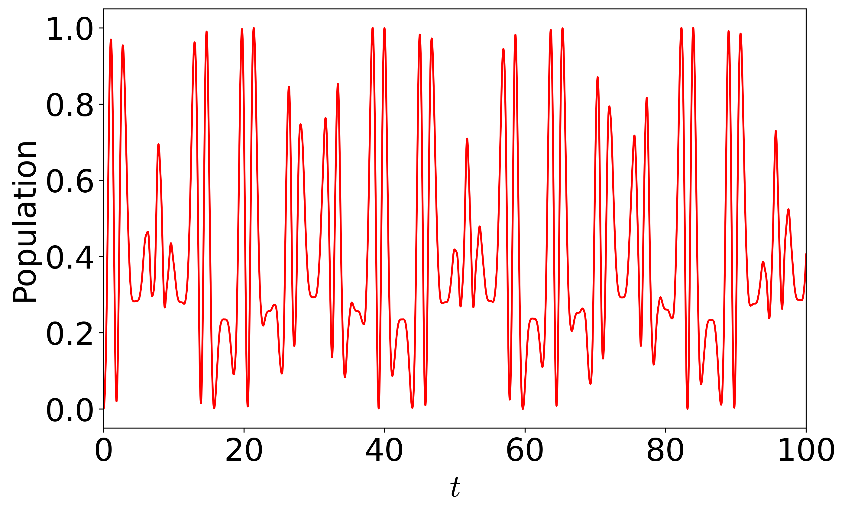
(IV)

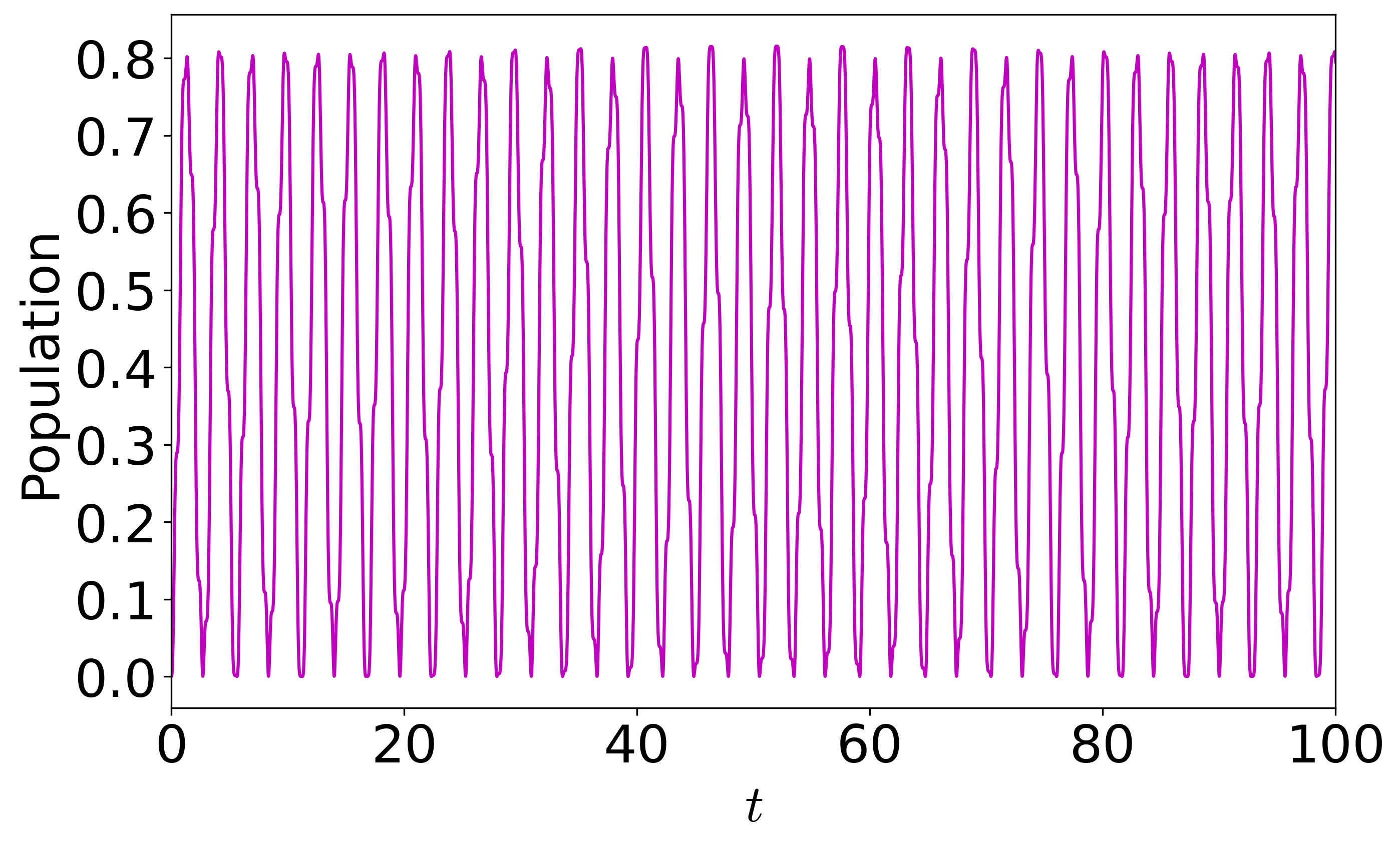
Figure 1: Populations of the excited state $|1\rangle$ for the four cases of parameters listed in Table 1. At time zero, all the populations are at the state $|0\rangle$.

Here, we consider a two state Hamiltonian with sinusoidal time dependences. Units are chosen such that $\hbar=1$ and the average level spacing and the average electronic coupling between two states are all equal to one. Thus, our Hamiltonian has the following form:

$$H(t) = \alpha_{1}\sin(\omega_{1}t)|1\rangle\langle 1|+(1+\alpha_{2}\sin(\omega_{2}t))|2\rangle\langle 2|$$ (51)

$$+ (1+\alpha_{c}\sin(\omega_{c}t))(|1\rangle\langle 2|+|2\rangle\langle 1|).$$

Although it is possible to introduce different phase factors within different sine functions, we do not consider such case since it does not appear to be important for the evaluation of numerical propagators. Even without such phase factors, the above Hamiltonian still has 6 parameters. For the test of approximate ME expressions, we chose four representative cases of parameters as listed in Table I.

For each case and each approximate expression, we calculated the propagator $U(t_{f},0)$ at $t_{f}=100$ by repeated application of the approximate expression $U(t_{k+1},t_{k})$, from the left, to $U(t_{k},0)$, starting from $U(0,0)={\rm I}$, until $k=N_{f}=t_{f}/\delta t$. All three fourth order expressions we have provided, Eqs. (18), (22), and (25), and our sixth order expression, Eq. (27), were tested along with other known fourth and sixth order expressions by Blanes et al.[26] and Iserles et al.[29] we have summarized.

Figure 1 shows time dependent populations at state $|2\rangle$ for the case where the initial state at time $t=0$ is $|1\rangle$. For the calculation of these populations, we used Eq. (25) for $\delta t=0.00610$, which offers accurate enough results for this demonstration. The time dependent population for each case shows a different beating structure reflecting the effects of time dependent change of the Hamiltonian components in addition to the intrinsic oscillation due to average off-diagonal coupling. As yet, due to the periodic nature of the time dependent Hamiltonian, all the populations exhibit periodic behavior at sufficiently long time. It is also clear that all the populations remain within $(0,1)$ as expected from a norm conserving propagator.

We also calculated errors in the propagator itself for each case. As a reference for the exact result, we used our sixth order method, Eq. (27), calculated with the choice of $\delta t=0.00610/8=0.0007625$. Then, for each method and choice of time step, we calculated an error defined as follows:

$${\rm error}=\frac{||U_{\rm approx}(t_{f})-U_{\rm ref}(t_{f})||_{F}}{||U_{\rm ref}(t_{f})||_{F}},$$ (52)

where the subscript F denotes the Frobenius norm defined by $||U||_{F}=\left(\sum_{i}\sum_{j}|U_{ij}|^{2}\right)^{\frac{1}{2}}$. The choice of time steps we tested are listed in Table 2.

(I)

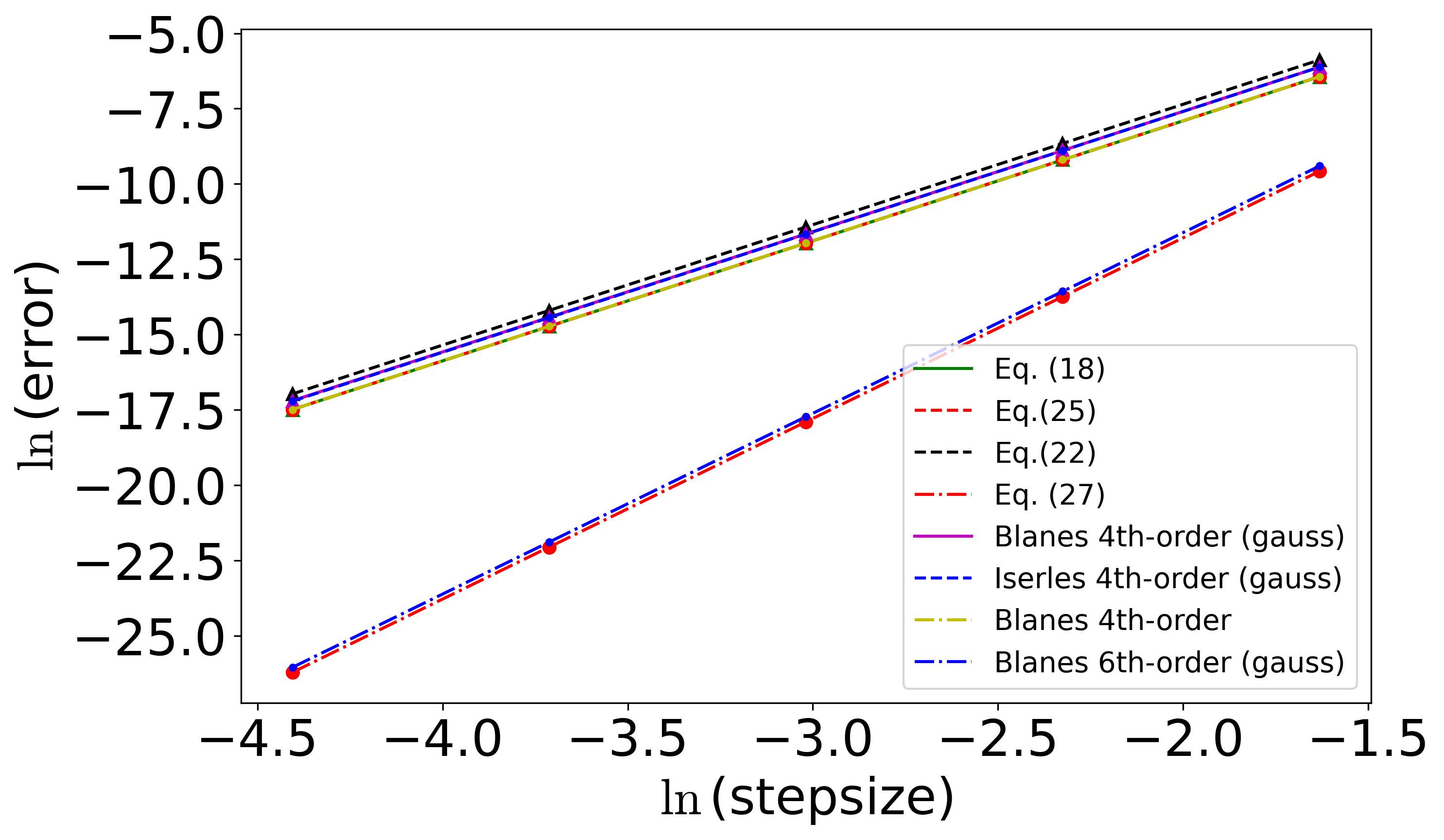
(II)

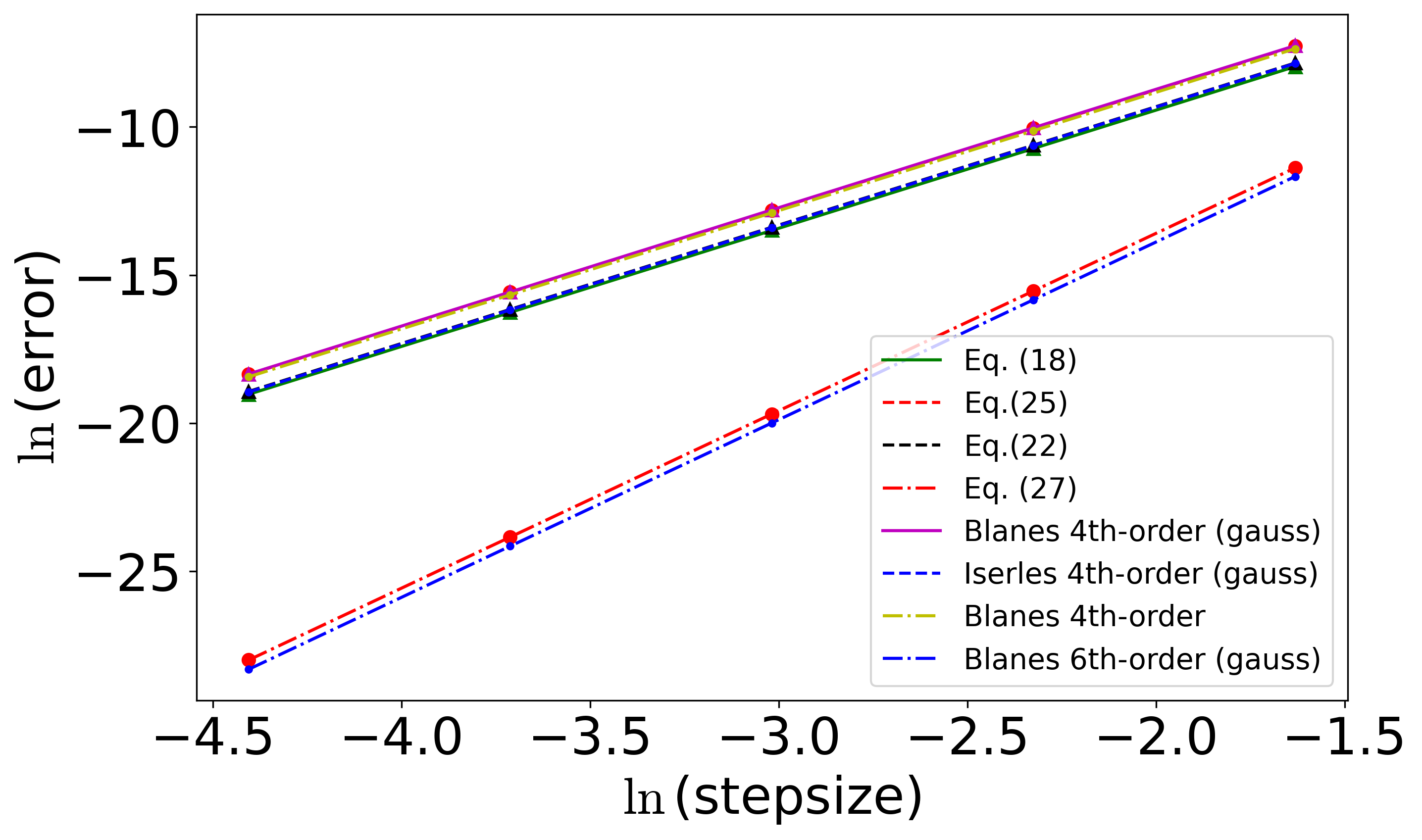
(III)

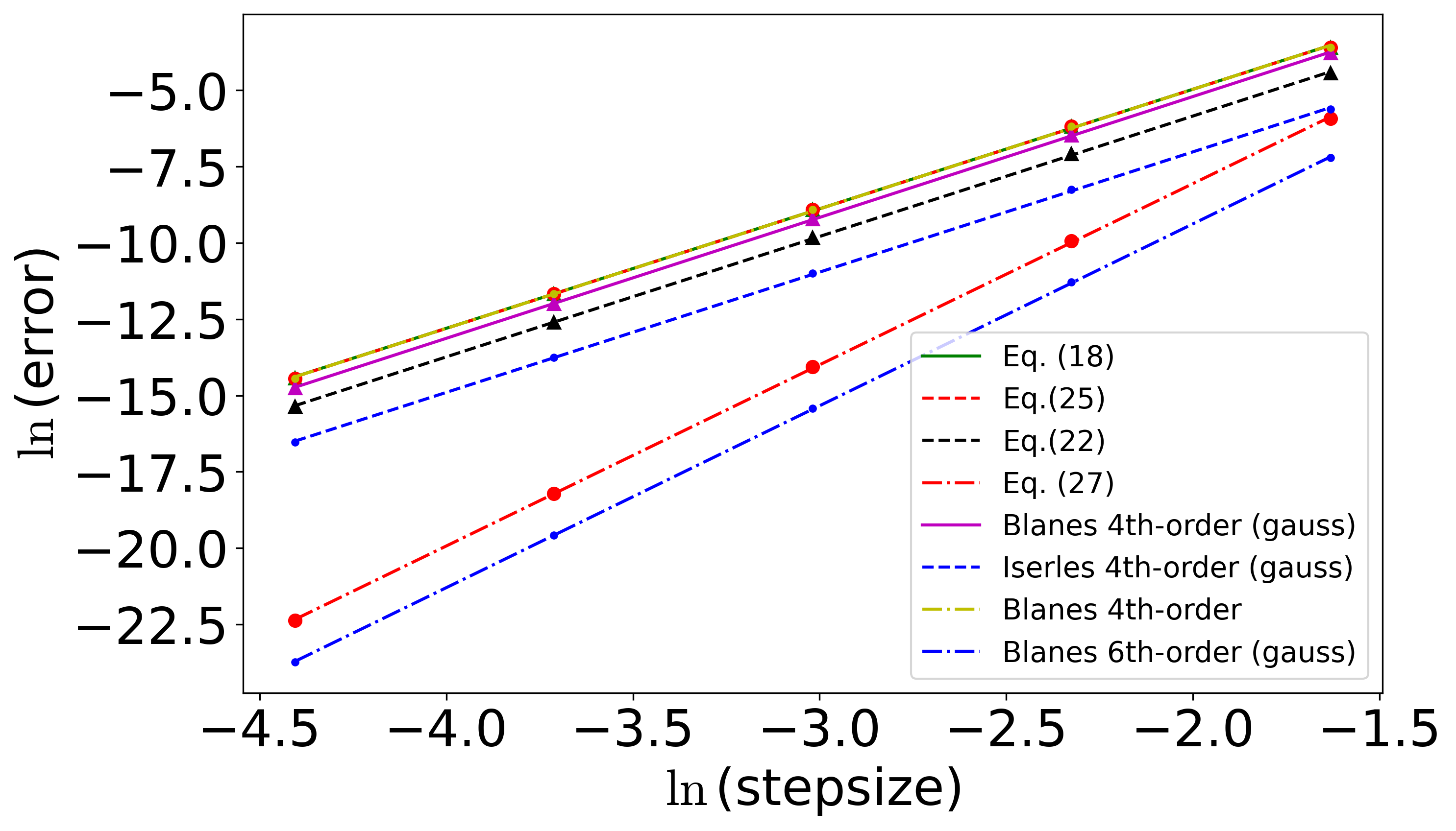
(IV)

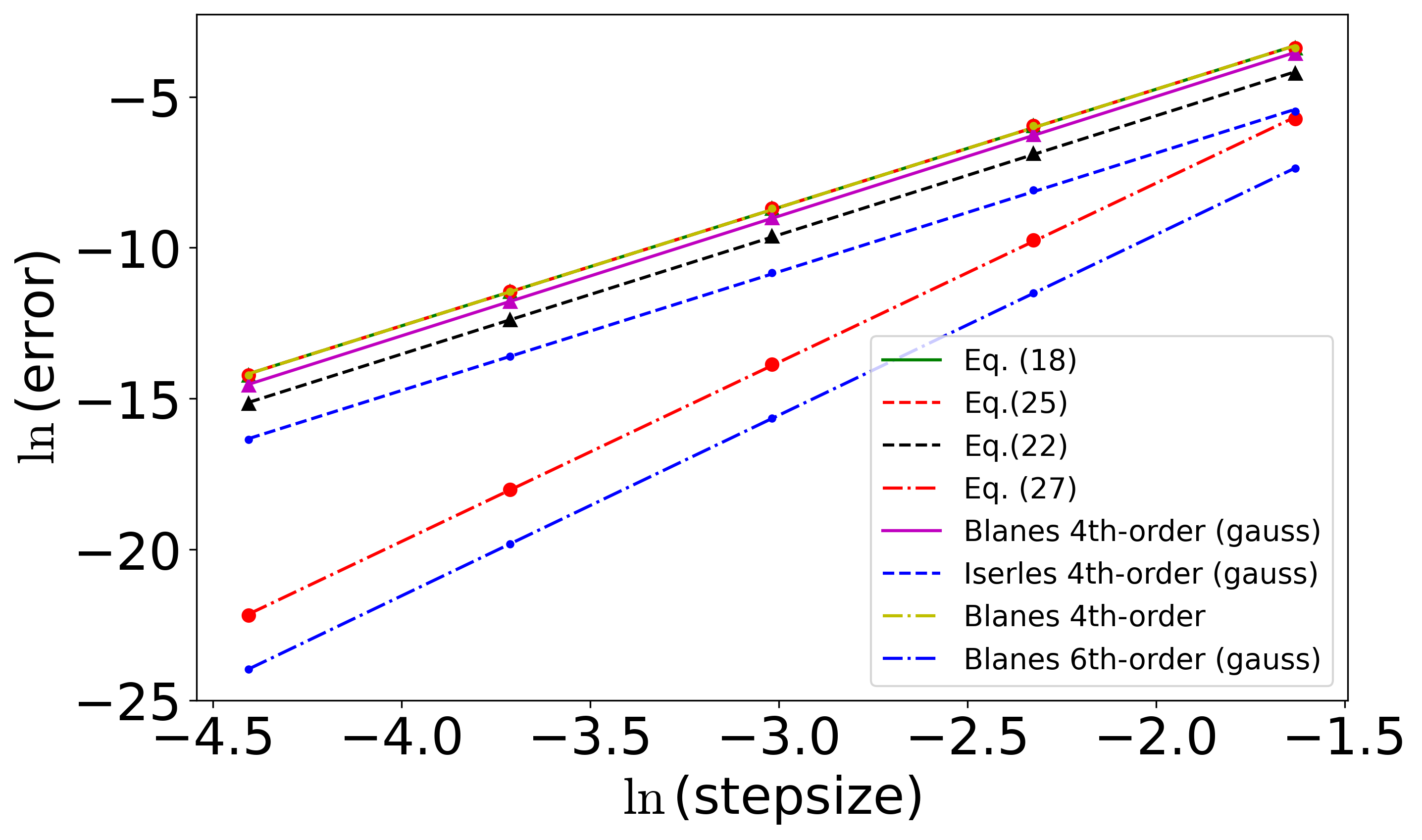
Figure 2: $\ln({\rm error})$ defined according to Eq. (52), vs. $\ln({\rm stepsize}=\delta t)$, for Eq. (51) based on different expressions for the four cases.

Figure 2 shows the errors calculated for our three fourth order expressions and the sixth order expression, and two fourth order expressions and sixth order expression by Blanes et al.[26] and a fourth order expression by Iserles et al..[29] Dots represent actual data of calculation and lines were drawn as guide. All the data exhibit expected scaling behavior with respect to the size of the time step, $\delta t$.

For cases I and II, the difference in errors between different fourth order expressions are marginal. The two sixth order expressions exhibit much more improved behavior and have similar performance. On the other hand, for cases III and IV where there is a high frequency oscillation, appreciable differences can be seen between different approximations. We find that our two fourth order expressions, Eqs. (18) and (25), show similar performance as the 4th order expression by Blanes et al. that uses simple integration scheme.[26] The 4th order expression with Gauss-Legendre quadrature by Blanes et al.[26] performs slightly better than the three expressions, but is worse than our 4th order expression with double commutator, Eq. (22).

Among the fourth order expressions, the expression by Iserles et al.,[29] which is also based on Gauss-Legendre quadrature, shows the best performance. However, this is the most expensive among all the fourth order expressions since it involves evaluation at two mid points, while the evaluation at two end points of the time interval is necessary for actual evaluation of physical observables, and since it also involves evaluation of double commutators. On the other hand, our best 4th order expression, Eq. (22), involves evaluation at only one mid point. Thus, Eq. (22) can be considered as a good choice when considering both efficiency and accuracy. In terms of simplicity and efficiency, Eq. (18) seems to be the best choice. It is interesting to note that the performance of this expression is comparable to that of Eq. (25), which is based on a higher order ME.

Of the two sixth order expressions, the expression by Blanes et al.[26], which is based on Gauss-Legendre quadrature, clearly performs better than our sixth order expression, (27), for cases III and IV. This shows the importance of accurate integration. However, further improvement of Eq. (27) is possible by incorporating similar quadrature of higher accuracy, making the latter comparable to former.

IV Conclusion

In this work, we have provided systematic approximations for the ME of the real time propagator for time dependent Hamiltonians, based on explicit integrations of Lagrange interpolation formula. We also tested their performance along with other existing expressions.[26, 29] All of these expressions rely on evaluation of Hamiltonians at discrete values of time and are applicable to any kind of time dependent Hamiltonian that can be approximated by low order polynomials within each time interval. We have tested these fourth order and sixth order expressions for a two-state Hamiltonian with sinusoidal time dependences, Eq. (51).

All the plots of errors with respect to the value of time step, $\delta t$, confirm their expected order of accuracy. Among the fourth order expressions, we find that Eq. (18) works fairly well considering its simplicity and efficiency. Although further test for other forms of Hamiltonian are still needed for more definite conclusion, the results provided here suggest that Eq. (18) can serve as a useful expression for a broad range of problems involving general time dependent Hamiltonian.

All the expressions derived and tested here can be employed for numerical time evolution for a broad class of time dependent Hamiltonians and thus can be utilized for calculating observables in time resolved spectroscopy, quantum control, and quantum sensing. Even when the Hamiltonian is independent of time, the approximate ME expressions can be used for solving the dynamics in the interaction picture with respect to a reference Hamiltonian. Similarly, they can also be utilized for the open system quantum dynamics when the reduced system density operator is solved in the interaction picture with respect to the zeroth order system Hamiltonian.

Table 2: Stepsize and number of points for numerical calculations.

Stepsize	Number of Points
0.00610	16384
0.01221	8192
0.02442	4096
0.04885	2048
0.09775	1024
0.19569	512

Appendix A Unitarity and symmetry of Magnus expansion

Since the time evolution operator $U_{\delta t}(t_{k+1},t_{k})$ should conserve the norm, it has to be unitary as follows:

$$U_{\delta t}^{\dagger}(t_{k+1},t_{k})U_{\delta t}(t_{k+1},t_{k})=U_{\delta t}(t_{k+1},t_{k})U_{\delta t}^{\dagger}(t_{k+1},t_{k})={\rm I},$$ (53)

where ${\rm I}$ is the identity operator. On the other hand, taking the Hermitian adjoint of Eq. (3), we find that

$$U_{\delta t}^{\dagger}(t_{k+1},t_{k})=\exp\left\{\sum_{n=1}^{\infty}\frac{1}{n!}\left(\frac{i}{\hbar}\right)^{n}M_{n}^{\dagger}(t_{k+1},t_{k})\right\}$$

$$=\exp\left\{\sum_{n=1}^{\infty}\frac{1}{n!}\left(-\frac{i}{\hbar}\right)^{n}(-1)^{n}M_{n}^{\dagger}(t_{k+1},t_{k})\right\}.$$ (54)

Note that each term of the ME in Eq. (3) satisfies the following property:

$$M_{n}^{\dagger}(t_{k+1},t_{k})=(-1)^{n-1}M_{n}(t_{k+1},t_{k}),$$ (55)

which can be verified directly for the expressions up to the fourth order shown in Eqs. (4) - (7) and be proven to be correct from the general nested commutator expression for the ME. Therefore, Eq. (54) becomes

$$U_{\delta t}^{\dagger}(t_{k+1},t_{k})=\exp\left\{-\sum_{n=1}^{\infty}\frac{1}{n!}\left(-\frac{i}{\hbar}\right)^{n}M_{n}(t_{k+1},t_{k})\right\}.$$ (56)

Since the exponent of the above operator is the same as $U_{\delta t}(t_{k+1},t_{k})$ except for the overall minus sign, the two operators commute and their exponents can be combined, which leads to the proof of unitarity as follows:

$$U_{\delta t}^{\dagger}(t_{k+1},t_{k})U_{\delta t}(t_{k+1},t_{k})=U_{\delta t}(t_{k+1},t_{k})U_{\delta t}^{\dagger}(t_{k+1},t_{k})$$

$$=\exp\left\{\sum_{n=1}^{\infty}\frac{1}{n!}\left(-\frac{i}{\hbar}\right)^{n}\left(M_{n}(t_{k+1},t_{k})-M_{n}(t_{k+1},t_{k})\right)\right\}$$

$$={\rm I}.$$ (57)

In fact, the above identity remains true even if the Magnus expansion is truncated at finite order because the symmetry property is satisfied by each term. This makes the finite order approximation of the Magnus expansion unitary.

On the other hand, since the Magnus expansion does not rely on any time ordering prescription, we expect that the same expansion is valid for the backward propagation with $t_{k}$ and $t_{k+1}$ exchanged. By definition, this backward propagator satisfies the following property:

$$U(t_{k})=U_{\delta t}(t_{k},t_{k+1})U(t_{k+1}).$$ (58)

This implies that

$$U_{\delta t}(t_{k},t_{k+1})=\exp\left\{\sum_{n=1}^{\infty}\frac{1}{n!}\left(-\frac{i}{\hbar}\right)^{n}M_{n}(t_{k},t_{k+1})\right\}$$

$$=\exp\left\{-\sum_{n=1}^{\infty}\frac{1}{n!}\left(-\frac{i}{\hbar}\right)^{n}M_{n}(t_{k+1},t_{k})\right\}=U^{\dagger}_{\delta}(t_{k+1},t_{k})$$

The above identity should remain true even if $\hbar$ is scaled by any numerical factor. This is possible only if each term satisfies the following symmetry property:

$$M_{n}(t_{k},t_{k+1})=-M_{n}(t_{k+1},t_{k}),$$ (60)

which can be confirmed directly for the expansions up to the fourth order, Eqs. (4)-(7). Let us assume that each term can be expanded with respect to $\delta t=t_{k+1}-t_{k}$ such that expansion coefficients are symmetric with respect to the exchange of $t_{k}$ and $t_{k+1}$ as follows:

$$M_{n}(t_{k+1},t_{k})=\sum_{j=0}^{\infty}\tilde{M}_{n}^{(j)}(t_{k+1},t_{k})\delta t^{j},$$ (61)

where $\tilde{M}_{n}^{(j)}(t_{k+1},t_{k})=\tilde{M}_{n}^{(j)}(t_{k},t_{k+1})$. In order for Eq. (60) to be satisfied, $\tilde{M}_{n}^{(j)}(t_{k},t_{k+1})$ with even $j$ should be zero. Therefore, Eq. (61) can be rewritten as

$$M_{n}(t_{k+1},t_{k})=\sum_{j=1}^{\infty}\tilde{M}_{n}^{(2j-1)}(t_{k+1},t_{k})\delta t^{2j-1}.$$ (62)

As a result, all the finite order Magnus expansions with symmetric coefficient as described above have always even order of accuracy with respect to $\delta t$. One simple way to achieve this property is to make Taylor series expansion of $M_{n}(t_{k+1},t_{k})$ around $(t_{k+1}+t_{k})/2$ with respect to $\delta t$. Alternatively, our expressions in the main text show that it can also be achieved through appropriate rearranging of terms starting from Lagrange interpolation expressions.

Appendix B B. Explicit calculation of low order ME terms

The first order approximation for the Hamiltonian, Eq. (10), can be expressed as

$$H^{(1)}(t)=H_{k}+\frac{(t-t_{k})}{\delta t}(H_{k+1}-H_{k})$$ (63)

When this approximation is used, the integrals involved in the evaluation of $M_{1}^{(1)}$ and $M_{2}^{(1)}$ can be calculated easily as follows:

$$\int_{t_{k}}^{t_{k+1}}d\tau H^{(1)}(\tau)=\frac{\delta t}{2}(H_{k}+H_{k+1}),$$ (64)

$$\int_{t_{k}}^{t_{k+1}}d\tau\int_{t_{k}}^{\tau}d\tau^{\prime}[H^{(1)}(\tau),H^{(1)}(\tau^{\prime})]=\frac{\delta t^{2}}{6}[H_{k+1},H_{k}].$$ (65)

For the evaluation of integral for $M_{3}^{(1)}$, we first expand the relevant Hamiltonians explicitly as follows:

$$[H^{(1)}(\tau),[H^{(1)}(\tau^{\prime}),H^{(1)}(\tau^{\prime\prime})]]+[H^{(1)}(\tau^{\prime\prime}),[H^{(1)}(\tau^{\prime}),H^{(1)}(\tau)]].$$

$$= [H_{k}+\frac{(\tau-t_{k})}{\delta t}(H_{k+1}-H_{k}),[H_{k}+\frac{(\tau^{\prime}-t_{k})}{\delta t}(H_{k+1}-H_{k}),H_{k}+\frac{(\tau^{\prime\prime}-t_{k})}{\delta t}(H_{k+1}-H_{k})]$$

$$\hskip 7.22743pt+[H_{k}+\frac{(\tau^{\prime\prime}-t_{k})}{\delta t}(H_{k+1}-H_{k}),[H_{k}+\frac{(\tau^{\prime}-t_{k})}{\delta t}(H_{k+1}-H_{k}),H_{k}+\frac{(\tau-t_{k})}{\delta t}(H_{k+1}-H_{k})]$$

$$= \frac{(t_{k+1}-\tau)(\tau^{\prime}-\tau^{\prime\prime})}{\delta t^{2}}[H_{k},[H_{k+1},H_{k}]]+\frac{(\tau-t_{k})(\tau^{\prime}-\tau^{\prime\prime})}{\delta t^{2}}[H_{k+1},[H_{k+1},H_{k}]]$$ (66)

$$\hskip 7.22743pt+\frac{(t_{k+1}-\tau^{\prime\prime})(\tau^{\prime}-\tau)}{\delta t^{2}}[H_{k},[H_{k+1},H_{k}]]+\frac{(\tau^{\prime\prime}-t_{k})(\tau^{\prime}-\tau)}{\delta t^{2}}[H(t_{k+1}),[H(t_{k+1}),H(t_{k})]]$$

Evaluation of the multiple time order integral in Eq. (6) with the the above integrand is now straightforward, for which we need integration of quadratic functions of time as follows:

$$\int_{t_{k}}^{t_{k+1}}d\tau\int_{t_{k}}^{\tau}d\tau^{\prime}\int_{t_{k}}^{\tau^{\prime}}d\tau^{\prime\prime}\frac{(t_{k+1}-\tau)(\tau^{\prime}-\tau^{\prime\prime})}{\delta t^{2}}$$

$$=\frac{1}{\delta t^{2}}\int_{t_{k}}^{t_{k+1}}(t_{k+1}-\tau)d\tau\int_{t_{k}}^{\tau}d\tau^{\prime}\int^{t_{k}}_{\tau^{\prime}}d\tau^{\prime\prime}(\tau^{\prime\prime}-\tau^{\prime})$$

$$=\frac{1}{\delta t^{2}}\int_{t_{k}}^{t_{k+1}}(t_{k+1}-\tau)d\tau\int_{t_{k}}^{\tau}d\tau^{\prime}\frac{(t_{k}-\tau^{\prime})^{2}}{2}$$

$$=\frac{1}{6\delta t^{2}}\int_{t_{k}}^{t_{k+1}}(t_{k+1}-\tau)(\tau-t_{k})^{4}d\tau$$

$$=-\frac{1}{6\delta t^{2}}(\frac{1}{5}\delta t^{5}-\frac{1}{4}\delta t^{5})=\frac{1}{120}\delta t^{3}$$ (67)

Similarly, other three time integrations can be evaluated as follows:

$$\int_{t_{k}}^{t_{k+1}}d\tau\int_{t_{k}}^{\tau}d\tau^{\prime}\int_{t_{k}}^{\tau^{\prime}}d\tau^{\prime\prime}\frac{(\tau-t_{k})(\tau^{\prime}-\tau^{\prime\prime})}{\delta t^{2}}=\frac{1}{30}\delta t^{3}$$ (68)

$$\int_{t_{k}}^{t_{k+1}}d\tau\int_{t_{k}}^{\tau}d\tau^{\prime}\int_{t_{k}}^{\tau^{\prime}}d\tau^{\prime\prime}\frac{(t_{k+1}-\tau^{\prime\prime})(\tau^{\prime}-\tau)}{\delta t^{2}}=-\frac{1}{30}\delta t^{3}$$ (69)

$$\int_{t_{k}}^{t_{k+1}}d\tau\int_{t_{k}}^{\tau}d\tau^{\prime}\int_{t_{k}}^{\tau^{\prime}}d\tau^{\prime\prime}\frac{(\tau^{\prime\prime}-t_{k+1})(\tau^{\prime}-\tau)}{\delta t^{2}}=-\frac{1}{120}\delta t^{3}$$ (70)

Combining all of them, we obtain the following simple expression:

$$\int_{t_{k}}^{t_{k+1}}d\tau\int_{t_{k}}^{\tau}d\tau^{\prime}\int_{t_{k}}^{\tau^{\prime}}d\tau^{\prime\prime}$$

$$\hskip 57.81621pt\Big{(}[H^{(1)}(\tau),[H^{(1)}(\tau^{\prime}),H^{(1)}(\tau^{\prime\prime})]]$$

$$\hskip 57.81621pt+[H^{(1)}(\tau^{\prime\prime}),[H^{(1)}(\tau^{\prime}),H^{(1)}(\tau)]]\Big{)}$$

$$=\frac{\delta t^{3}}{40}[H_{k+1}-H_{k},[H_{k+1},H_{k}]].$$ (71)

Now let us consider the quadratic approximation for the Hamiltonian, Eq. (11), which can be expressed as

$$H^{(2)}(\tau) = H_{k}+\frac{\tau-t_{k}}{\delta t}\left(-3H_{k}+4H_{k+\frac{1}{2}}-H_{k+1}\right)$$ (72)

$$+2\frac{(\tau-t_{k})^{2}}{\delta t^{2}}\left(H_{k}-2H_{k+\frac{1}{2}}+H_{k+1}\right).$$

Employing the above approximation, the integral for $M_{1}^{(2)}$ can be calculated as follows:

$$\int_{t_{k}}^{t_{k+1}}d\tau H^{(2)}(\tau)=\frac{\delta t}{6}(H_{k}+4H_{k+\frac{1}{2}}+H_{k+1}).$$ (73)

For the evaluation of $M_{2}^{(2)}$, let us first consider $[H^{(2)}(\tau),H^{(2)}(\tau^{\prime})]$, which can be explicitly calculated and rearranged to have the following expression:

$$[H^{(2)}(\tau),H^{(2)}(\tau^{\prime})] = \left([H_{k+1},H_{k}]-2[H_{k+\frac{1}{2}},H_{k}]\right)\left(\frac{2}{\delta t^{2}}(\tau-t_{k})^{2}-\frac{2}{\delta t^{2}}(\tau^{\prime}-t_{k})^{2}\right)$$ (74)

$$+\left(-2[H_{k},H_{k+\frac{1}{2}}]+2[H_{k},H_{k+1}]-2[H_{k+\frac{1}{2}},H_{k}]\right)$$

$$\hskip 36.135pt\times\frac{2}{\delta t^{3}}\left((\tau-t_{k})^{2}(\tau^{\prime}-t_{k})-(\tau-t_{k})(\tau^{\prime}-t_{k})^{2}\right)$$

$$+\left(4[H_{k+\frac{1}{2}},H_{k}]-[H_{k+1},H_{k}]\right)\frac{1}{\delta t}\left((\tau-t_{k})-(\tau^{\prime}-t_{k})\right).$$

All the time integrations involving $\tau$ and $\tau^{\prime}$ can be performed easily as follows:

$$\frac{2}{\delta t^{2}}\int_{t_{k}}^{t_{k+1}}\int_{t_{k}}^{\tau}d\tau^{\prime}\left\{(\tau-t_{k})^{2}-(\tau^{\prime}-t_{k})^{2}\right\}=\frac{1}{3}\delta t^{2}$$ (75)

$$\frac{2}{\delta t^{3}}\int_{t_{k}}^{t_{k+1}}d\tau\int_{t_{k}}^{\tau}d\tau^{\prime}\left\{(\tau-t_{k})^{2}(\tau^{\prime}-t_{k})\right.\hskip 36.135pt$$

$$\left.\hskip 36.135pt-(\tau-t_{k})(\tau^{\prime}-t_{k})^{2}\right\}=\frac{1}{15}\delta t^{2}$$ (76)

$$\frac{1}{\delta t}\int_{t_{k}}^{t_{k+1}}d\tau\int_{t_{k}}^{\tau}d\tau^{\prime}\left\{(\tau-t_{k})-(\tau^{\prime}-t_{k})\right\}=\frac{1}{6}\delta t^{2}$$ (77)

Therefore, we find that

$$\int_{t_{k}}^{t_{k}+1}\int_{t_{k}}^{\tau}d\tau^{\prime}d\tau[H^{(2)}(\tau),H^{(2)}(\tau^{\prime})]$$

$$=\left([H_{k+1},H_{k}]-2[H_{k+\frac{1}{2}},H_{k}]\right)\frac{\delta t^{2}}{3}$$

$$+\left(-2[H_{k},H_{k+\frac{1}{2}}]+2[H_{k},H_{k+1}]-2[H_{k+\frac{1}{2}},H_{k+1}]\right)\frac{\delta t^{2}}{15}$$

$$+\left(4[H_{k+\frac{1}{2}},H_{k}]-[H_{k+1},H_{k}]\right)\frac{\delta t^{2}}{6}$$

$$=\frac{\delta t^{2}}{30}\left([H_{k+1},H_{k}]+4[H_{k+\frac{1}{2}},H_{k}]+4[H_{k+1},H_{k+\frac{1}{2}}]\right)$$

$$=\frac{\delta t^{2}}{30}[H_{k}+4H_{k+\frac{1}{2}},H_{k}-H_{k+1}].$$ (78)

Appendix C Verification of the fourth order commutator expression

For the simplification of $M_{4}^{(1)}$, we guessed a simplified form that involves an undetermined coefficient $c$ and solved the quadratic equation for $c$ such that it reproduces the original expression. The resulting expression for the relevant integral is as follows:

$$\int_{t_{k}}^{t_{k+1}}d\tau\int_{t_{k}}^{\tau}d\tau^{\prime}\int_{t_{k}}^{\tau^{\prime}}d\tau^{\prime\prime}\int_{t_{k}}^{\tau^{\prime\prime}}d\tau^{\prime\prime\prime}$$

$$\hskip 57.81621pt\Big{(}[[[H^{(1)}(\tau),H^{(1)}(\tau^{\prime})],H^{(1)}(\tau^{\prime\prime})],H^{(1)}(\tau^{\prime\prime\prime})]$$

$$\hskip 57.81621pt+[H^{(1)}(\tau),[[H^{(1)}(\tau^{\prime}),H^{(1)}(\tau^{\prime\prime})],H^{(1)}(\tau^{\prime\prime\prime})]]$$

$$\hskip 57.81621pt+[H^{(1)}(\tau),[H^{(1)}(\tau^{\prime}),[H^{(1)}(\tau^{\prime\prime}),H^{(1)}(\tau^{\prime\prime\prime})]]]$$

$$\hskip 57.81621pt+[H^{(1)}(\tau^{\prime}),[H^{(1)}(\tau^{\prime\prime}),[H^{(1)}(\tau^{\prime\prime\prime}),H^{(1)}(\tau)]]]\Big{)}$$

$$=\frac{\delta t^{4}}{420}[\frac{1}{c}H_{k}-H_{k+1},[H_{k+1}-cH_{k},[H_{k+1},H_{k}]]],$$ (79)

where $c=-\frac{5-\sqrt{21}}{2}$. Note that the choice of $c$ is not unique because the algebraic equation under-determined. We also verified this expression using a computer algebra system known as SymPy.[31]

The steps to verify Eq. (79) are as follows:

1) Importing sympy and declaring the variables found in Eq. (79).

⬇

import sympy as sp

H = sp.Function(’H’,commutative=False)

t, t_0 = sp.symbols("t t_0",constant=True)

tau_1, tau_2, tau_3, tau_4 = sp.symbols(’tau_1 tau_2 tau_3 tau_4’)

2) Coding the commutators and integrals on the LHS of Eq.(79) as follows:

⬇

from sympy.physics.quantum import Commutator

int_1 = 0

int_1 += Commutator(Commutator(Commutator(H(tau_1),H(tau_2)),H(tau_3)),H(tau_4))

int_1 += Commutator(H(tau_1),Commutator(Commutator(H(tau_2),H(tau_3)),H(tau_4)))

int_1 += Commutator(H(tau_1),Commutator(H(tau_2),Commutator(H(tau_3),H(tau_4))))

int_1 += Commutator(H(tau_2),Commutator(H(tau_3),Commutator(H(tau_4),H(tau_1))))

int_1 *= sp.Rational(1,12)

integral = sp.Integral(int_1,(tau_4,t_0,tau_3))

integral= sp.Integral(integral,(tau_3,t_0,tau_2))

integral = sp.Integral(integral,(tau_2,t_0,tau_1))

integral= sp.Integral(integral,(tau_1,t_0,t))

3) Define the linearization function equivalent to Eq. (63), apply it to the integral, and simplify the expression:

⬇

def linearization(tau):

return H(t_0) + ((tau-t_0)/(t-t_0) * (H(t)-H(t_0)))

result = integral.replace(lambda x:x.func==H, lambda x:linearization((x.args[0])),simultaneous=True)

result = result.expand().doit(manual=True).simplify()

result = result.subs(t_0,0,simultaneous=True).simplify()

4) Code the RHS of Eq. (79) and test for equality. In SymPy, equality testing is done by subtracting the two expressions and simplifying. The last line of code prints this difference, which will equal zero for equivalent expressions.

⬇

c = sp.symbols(’c’)

RHS = sp.expand(Commutator(-1/c*H(0)+1*H(t),Commutator(c*H(0)+-1*H(t),

Commutator(H(t),H(0)))))/5040*t**4

RHS = RHS.subs(c, sp.Rational(-5,2) - sp.sqrt(21)/2).doit()

#RHS = RHS.subs(c,sp.Rational(-5,2) + sp.sqrt(21)/2).doit() #alternative value for c

print((result - RHS).simplify())

References

- Mukamel [1995] Mukamel, S. Principles of Nonlinear Spectroscopy; Oxford University Press: New York, 1995.
- Cina [2022] Cina, J. A. Getting Started on Time-Resolved Molecular Specrtoscopy; Oxford University Press: Oxford, 2022.
- Burghardt and Stefan Haacke [2017] Burghardt, I.; Stefan Haacke, E. Ultrafast Dynamics at the Nanoscale: Biomolecules and Supramolecular Assemblies; Pan Stanford Publishing: Singapore, 2017.
- Jang [2020] Jang, S. J. Dynamics of Molecular Excitons (Nanophotonics Series); Elsevier: Amsterdam, 2020.
- Shapiro and Brumer [2013] Shapiro, M.; Brumer, P. Quantum control of molecular processes, 2nd edition; Wiley-VCH: Weinheim, 2013.
- Singh [2019] Singh, P. Sixth-order schemes for laser-matter interaction in the Schrödinger equation. J. Chem. Phys. 2019, 150, 154111.
- Hu et al. [2020] Hu, W.; Gu, B.; Franco, I. Toward the laser control of electronic decoherence. J. Chem. Phys. 2020, 152, 184305.
- Degen et al. [2017] Degen, C. L.; Reinhard, F.; Capellaro, P. Quantum sensing. Rev. Mod. Phys. 2017, 89, 035002.
- Jang et al. [2008] Jang, S.; Cheng, Y.-C.; Reichman, D. R.; Eaves, J. D. Theory of coherent resonance energy transfer. J. Chem. Phys. 2008, 129, 101104.
- Jang [2009] Jang, S. Theory of coherent resonance energy transfer for coherent initial condition. J. Chem. Phys. 2009, 131, 164101.
- Jang [2011] Jang, S. Theory of multichromophoric coherent resonance energy transfer: A polaronic quantum master equation approach. J. Chem. Phys. 2011, 135, 034105.
- Jang et al. [2013] Jang, S.; Berkelbach, T.; Reichman, D. R. Coherent quantum dynamics in donor-bridge-acceptor nonadiabatic processes: Beyond the hopping and super-exchange mechanisms. New J. Phys. 2013, 15, 105020.
- Jang [2022] Jang, S. J. Partially polaron-transformed quantum master equation for exciton and charge transport dynamics. J. Chem. Phys 2022, 157, 104107.
- Montoya-Castillo et al. [2017] Montoya-Castillo, A.; Berkelbach, T. C.; Reichman, D. R. Extending the applicability of Redfield theories into highly non-Markovian regimes. J. Chem. Phys. 2017, 143, 194108.
- Mulvihill and Geva [2022] Mulvihill, E.; Geva, E. Simulating the dynamics of electronic observables via reduced-dimensionality generalized quantum master equations. J. Chem. Phys. 2022, 156, 044119.
- Schulman [1981] Schulman, L. S. Techniques and Applications of Path Integration; Wiley-Interscience: New York, 1981.
- Trotter [1958] Trotter, E. On the products of semi-groups of operators. Proc. Am. Math. Soc. 1958, 10, 545.
- Suzuki [1985] Suzuki, M. Decomposition formulas of exponential operators and Lie exponentials with some applications to quantum mechanics and statistical mechanics. J. Math. Phys. 1985, 26, 601.
- Suzuki [1997] Suzuki, M. Compact exponential product formulas and operator functional derivative. J. Math. Phys. 1997, 38, 1183.
- Jang et al. [2001] Jang, S.; Jang, S. M.; Voth, G. A. Application of higher order composite factorization schemes in imaginary time path integral simulations. J. Chem. Phys. 2001, 115, 7832.
- Chin [1997] Chin, S. A. “Symplectic integrators from composite operator factorizations”. Phys. Lett. A 1997, 226, 344.
- Chin and Chen [2002] Chin, S. A.; Chen, C. R. Gradient symplectic algorithms for solving the Schrödinger equation with time dependent potentials. J. Chem. Phys. 2002, 117, 1409.
- Magnus [1954] Magnus, W. On the exponential solution of differential equations for a linear operator. Comm. Pure Appl. Math. 1954, 7, 649–673.
- Pechukas and Light [1966] Pechukas, P.; Light, J. C. On the exponential form of time-displacement operators in quantum mechanics. J. Chem. Phys. 1966, 44, 3897–3912.
- Blanes et al. [2009] Blanes, S.; Casas, F.; Oteo, J. A.; Ros, J. The Magnus expansion and some of its applications. Phys. Rep. 2009, 470, 151–238.
- Blanes et al. [2000] Blanes, S.; Casas, F.; Ros, J. Improved higher order propagators based on the Magnus expansion. BIT Numer. Math. 2000, 40, 434–450.
- Munthe–Kaas and Owren [1999] Munthe–Kaas, H.; Owren, B. Computations in a free Lie algebra. Phil. Trans. RSC A: Math. Phys. Eng. Sci. 1999, 357, 957–981.
- Blanes et al. [2002] Blanes, S.; Casas, F.; Ros, J. Higher order optimized geometric integrators for linear differential equations. BIT Numer. Math. 2002, 42, 262–284.
- Iserles and Nørsett [1999] Iserles, A.; Nørsett, S. P. On the solution of linear differential equations in Lie groups. Phil. Trans. RSC A: Math. Phys. Eng. Sci. 1999, 357, 983–1019.
- Klarsfield and Oteo [1989] Klarsfield, S.; Oteo, J. A. Recursive generation of higher order terms in the Magnus expansion. Phys. Rev. A 1989, 39, 3270–3270.
- Meurer et al. [2017] Meurer, A. et al. SymPy: symbolic computing in Python. PeerJ Comput. Sci. 2017, 3, e103.