Rethinking Multiple Instance Learning for Whole Slide Image Classification: A Bag-Level Classifier is a Good Instance-Level Teacher

Abstract

Multiple Instance Learning (MIL) has demonstrated promise in Whole Slide Image (WSI) classification. However, a major challenge persists due to the high computational cost associated with processing these gigapixel images. Existing methods generally adopt a two-stage approach, comprising a non-learnable feature embedding stage and a classifier training stage. Though it can greatly reduce the memory consumption by using a fixed feature embedder pre-trained on other domains, such scheme also results in a disparity between the two stages, leading to suboptimal classification accuracy. To address this issue, we propose that a bag-level classifier can be a good instance-level teacher. Based on this idea, we design Iteratively Coupled Multiple Instance Learning (ICMIL) to couple the embedder and the bag classifier at a low cost. ICMIL initially fix the patch embedder to train the bag classifier, followed by fixing the bag classifier to fine-tune the patch embedder. The refined embedder can then generate better representations in return, leading to a more accurate classifier for the next iteration. To realize more flexible and more effective embedder fine-tuning, we also introduce a teacher-student framework to efficiently distill the category knowledge in the bag classifier to help the instance-level embedder fine-tuning. Thorough experiments were conducted on four distinct datasets to validate the effectiveness of ICMIL. The experimental results consistently demonstrate that our method significantly improves the performance of existing MIL backbones, achieving state-of-the-art results. The code is available at: https://github.com/Dootmaan/ICMIL/tree/confidence_based

Multiple instance learning, Whole slide image, Weakly-supervised learning, Deep learning.

1 Introduction

Whole Slide Images (WSIs), which are biomedical images scanned at the microscopic level, have become extensively utilized in cancer diagnosis [1]. Compared to traditional microscope-based observation, WSIs offer advantages such as easier storage and analysis. However, their high-resolution nature presents challenges for computer-aided automatic analysis [2, 3], as the currently limited GPU memory makes it infeasible to directly apply existing classification networks to these gigapixel images. To tackle this issue, a widely adopted approach is the patch-based learning scheme [4, 5, 6], which involves dividing a WSI into multiple small patches and training an end-to-end classification network exclusively on the patch level. Although the patch-level training consumes much less GPU memory, acquiring precise and comprehensive patch-level annotations for WSIs is prohibitively expensive due to their large size and resolution [7].

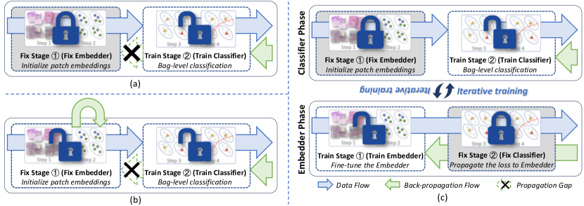
Figure 1: Comparison between different MIL pipelines and our proposed ICMIL. (a) Ordinary MIL pipeline that uses a fixed patch embedder for patch feature extraction. There is a semantic gap between the embedder and the classifier in these methods because the embedder cannot be fine-tuned on the WSI data. (b) MIL pipelines that involve self-supervised fine-tuning of the patch embedder. Although the domain shift problem is mitigated in this way, there is still a semantic gap between the two stages of MIL since their training processes are separated and have no information exchange. (c) The proposed ICMIL pipeline, which consists of two training phases that can iteratively couple the two stages in MIL backbones. It solves the domain shift problem, and enables information exchange in the MIL backbones.

Therefore, MIL, as a weakly-supervised learning scheme that only requires slide-level labels, has become more and more widely used recently [8]. MIL methods treat each WSI as a bag, and consider the tiled non-overlapping patches within the WSI as the instances in the bag. A bag is classified as positive if at least one of its instances is positive, and as negative only if all instances are negative. To facilitate cost-effective training, the common pipeline for MIL-based WSI analysis typically consists of two stages as shown in Fig. 1(a). The first stage is a non-learnable patch embedding stage, including tiling the gigapixel WSI into small non-overlapping patches and embedding them into feature vectors through a frozen patch embedder pre-trained on ImageNet [9]. The second stage is a trainable classification stage, comprising of aggregating the instance representations into bag-level representations and training a bag-level classifier on them. Although employing a frozen patch embedder reduces GPU memory consumption significantly, it also introduces a domain shift to the MIL classification model. Additionally, treating the embedding stage and the classification stage as two unrelated processes can also lead to lack of information exchange within the MIL pipeline, causing inconsistencies. Recent approaches have been proposed to fine-tune the patch embedder using task-agnostic methods, such as self-supervised techniques [10, 11, 12] or weakly-supervised techniques [13, 14, 15]. However, as these two stages are still trained separately with different supervision signals, they lack joint optimization and still may cause inconsistencies in the MIL pipeline.

To address this issue, we propose that the bag-level classifier is a good instance-level teacher, which can be used to help in fine-tuning the embedder by guiding the generation of the instance pseudo-labels. Based on this idea, we develop ICMIL, a simple yet effective method that establishes a connection between the bag classifier and the patch embedder through an iterative optimization scheme. As shown in Fig. 1(c), ICMIL consists of two phases. In the first phase (i.e., Classifier Phase), the patch embedder is frozen, and the subsequent aggregator and classifier are trained based on the instance representations generated by the embedder. In the second phase (i.e., Embedder Phase), the aggregator and the classifier are frozen, and the patch embedder is fine-tuned using instance-level pseudo-labels generated under the guidance of the bag-level classifier. To facilitate flexible and efficient embedder fine-tuning, we introduce a teacher-student-based method to enhance the knowledge distillation process from the bag-level classifier to the instance-level embedder. This method considers the bag-level classifier as the teacher of a hidden instance-level classifier, leveraging the category knowledge in the bag-level classifier to guide the instance-level embedder fine-tuning. When Embedder Phase is finished, ICMIL returns to Classifier Phase with the newly fine-tuned embedder, aiding in the training of a more accurate bag-level classifier, thereby improving the overall performance of the MIL backbone on the WSI dataset. If the desired model performance is not achieved, the iteration process can be repeated to ensure stronger coupling.

The preliminary version of ICMIL [16] was presented as a conference paper at the 26th International Conference on Medical Image Computing and Computer Assisted Intervention (MICCAI 2023). This extended work brings significant improvements, including proposing a new confidence-based embedder fine-tuning method for Embedder Phase, a novel bag augmentation method for Classifier Phase, and providing substantial extra experimental studies on four datasets. In summary, our contributions are: (1) We propose ICMIL, which can mitigate the domain shift and semantic gap problems in existing MIL backbones by iteratively coupling the bag classifier and the patch embedder in MIL methods during training. (2) We propose a confidence-based teacher-student approach to achieve effective and robust knowledge transfer from the bag-level classifier to the instance-level patch embedder, realizing weakly-supervised patch embedder fine-tuning. (3) We conduct thorough experiments with three representative MIL backbones on four datasets, and demonstrate the effectiveness of ICMIL.

2 Related Works

2.1 Multiple Instance Learning on WSI

MIL has gained increasing popularity as an efficient solution for WSI classification, as it solely requires slide-level labels [17, 11] for training. In MIL methods, an ImageNet pre-trained feature embedder is typically employed to convert the $K$ patches within a WSI into $K$ feature vectors. This conversion significantly reduces the spatial dimensions from gigapixel to $K$$\times$$M$, where $M$ represents the dimensionality of the feature vectors. Subsequently, an aggregation module is utilized to fuse the $K$ feature vectors into a single 1$\times$$M$ feature vector, effectively representing the entire WSI. By training a bag-level classifier based on these feature vectors, the model can predict the category of the corresponding WSI at a low computational cost.

Max pooling and mean pooling are two widely used aggregation methods, but their simple mechanisms can also lead to sub-optimal performance. For instance, mean pooling has the potential to diminish the distinction between negative and positive instances, while max pooling may occasionally overlook the most discriminative patch-level instance. To address these limitations, Attention-based MIL (ABMIL) [18] was proposed. ABMIL introduces a learnable aggregator that generates bag-level representations by utilizing attention scores assigned to the instance representations. Building upon this work, CLAM [17] was subsequently proposed, incorporating additional clustering branches for the bag-level classifier. Recent researches have also focused on leveraging the inter-instance information during the aggregation process. For instance, TransMIL [19] proposed to use the self-attention mechanism [20] to model the relationships between instances, and DSMIL [11] introduced a comprehensive multi-scale embedding fusion technique to generate more comprehensive patch representations.

2.2 Embedder Fine-tuning in MIL

In conventional MIL pipelines, the patch embedding stage and the classification stage are considered as separated and unrelated processes [17, 18, 21, 19, 22]. When extracting features from gigapixel WSIs with limited GPU memory, it is common practice to bypass training the embedder and instead utilize a pre-trained model from ImageNet for feature extraction [17, 18, 21, 19, 22]. However, this approach gives rise to a domain shift problem as the natural images in ImageNet can significantly differ from medical WSIs. Moreover, the two-stage training process introduces a semantic gap within the MIL pipeline, potentially compromising classification accuracy. Presently, the most prevalent solutions to address domain shift challenges in MIL are task-agnostic fine-tuning methods based on Weakly-Supervised Learning (WSL) and Self-supervised Learning (SSL). In the ItS2CLR method [13], the authors propose generating instance-level pseudo-labels based on the aggregator attention score. Subsequently, instances with the top-k or bottom-k scores are considered positive or negative instances, respectively, for fine-tuning the embedder. Another approach, DSMIL [11], employs self-supervised learning based on the SimCLR technique [23], enabling task-agnostic fine-tuning of the embedder.

However, despite these fine-tuning methods, the issue of broken loss back-propagation from the classification stage to the embedding stage persists in MIL pipelines. Consequently, task-specific fine-tuning of the patch embedder remains unrealized, leading to potential imperfections in optimizing the entire MIL pipeline. Figure 1 provides an intuitive comparison of different MIL pipeline designs. As depicted, conventional MIL pipelines overlook the domain shift problem and the semantic gap issue, relying on independent feature extraction, which significantly compromises model performance. On the other hand, MIL combined with WSL/SSL incorporates weak-supervision or self-supervision during patch embedder training, partially mitigating the domain shift problem. Nevertheless, since the fine-tuning process is separate from MIL training, it merely enables task-agnostic fine-tuning and fails to address the semantic gap between the embedder and the classifier in MIL. In contrast, our proposed method, ICMIL, effectively addresses this issue by establishing loss propagation from the classifier to the embedder, thus realizing task-specific fine-tuning of the embedder.

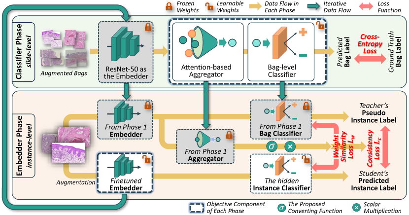
Figure 2: A detailed view of the pipeline of ICMIL with confidence-based embedder fine-tuning method. The classic ABMIL is used as the ICMIL backbone for the example.

3 Methodology

3.1 Overview of ICMIL

The fundamental concept of ICMIL is inspired by the classical machine learning technique, Expectation-Maximization (EM). EM is an iterative optimization method commonly used in problems involving hidden variables. Similarly, in MIL pipelines, we consider the instance representations obtained from the patch embedder as a hidden variable. Correspondingly in ICMIL, Classifier Phase optimizes the bag-level classifier based on the estimation of this hidden variable, and Embedder Phase fine-tune the embedder by maximizing the likelihood of the classifier’s predictions, so the hidden variable can be re-estimated in the next iteration.

To ensure the successful implementation of the fine-tuning scheme in Embedder Phase of ICMIL, it is essential for the bag-level representations and the instance-level representations to reside in the same latent space. This requirement is met by most MIL backbones, as their bag-level representations are derived from a linear combination of the instance representations. It is also advisable to use relatively simple aggregators in the MIL backbone to avoid introducing unnecessary complexity. Overly complex aggregators can lead to more significant disparities between the decision boundaries of the bag-level classifier and the hidden instance-level classifier. Consequently, this misalignment may introduce additional noise in the pseudo-labels during the fine-tuning of the embedder and slow down the convergence.

Different from previous works that solely utilize EM as a supportive tool for training either the patch embedder [24, 25] or the bag-level classifier [13], we are the first to consider the entire MIL pipeline as an EM-like problem. It is important to note that while ICMIL draws inspiration from EM, its practical implementation incorporates unique designs that go beyond the traditional EM concept. For instance, in ICMIL, we perform two iterative optimization processes at two different scales, namely the slide level and the patch level. Furthermore, our optimization process differs from the traditional EM approach as we introduce a teacher-student-based framework during the instance-level embedder fine-tuning phase to mitigate the noise in the pseudo-labels. These modifications result in substantial differences in the mathematical expression and overall methodology of ICMIL compared to the original EM method, and to facilitate a better understanding, we will introduce the detailed pipeline of ICMIL based on the classic ABMIL backbone in the following paragraphs.

3.2 Classifier Phase

A schematic view of Classifier Phase in ICMIL is depicted in the upper section of Fig. 2. In Classifier Phase, the primary objective is to train a bag-level classifier based on the fixed patch embedder. Since ICMIL is a framework that can suit different MIL methods, this phase can be implemented based on many existing MIL backbones, such as Max Pooling-based MIL, ABMIL, and DTFD-MIL. Nonetheless, to further improve the generalization ability of the MIL backbones, we also propose to use a pseudo-bag + bag mix-up scheme as data augmentation for this phase.

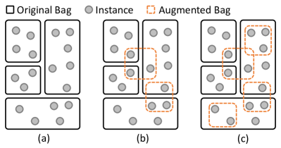
Figure 3: Comparison of different augmentation methods. (a) The original dataset without augmentation. (b) Dataset after bag mix-up augmentation method. (c) Dataset after mix-up + pseudo-bag augmentation.

3.2.1 Bag Augmentation

Different from ordinary image augmentation methods on the instance level, we propose to use the more efficient bag-level augmentation on WSIs. Inspired from [26, 27, 28], we integrate the bag mix-up method with the pseudo-bag augmentation scheme, resulting in a higher generalization ability of the MIL model.

The mathematical expression of the augmentation method can be described as follows. Without loss of generality, let $(A,B)$ denote any pair of bags from the original dataset that $A\neq B$, and $y_{A},y_{B}$ represent their labels. After partition, let $\{a_{1},a_{2},...,a_{n}\}$ and $\{b_{1},b_{2},...,b_{n}\}$ refer to their pseudo-bags respectively, where $n$ is a hyper-parameter set to 4 by default. We choose not to use a large $n$ because it can increase the possibility of a true-negative pseudo-bag inheriting the false-positive label. Then, we randomly mask $\lfloor\lambda\cdot n\rfloor$ bags in $A$ and $\lceil(1-\lambda)\cdot n\rceil$ in $B$ through a Beta distribution, i.e., $\lambda\sim Beta(\alpha,\alpha)$ and $\alpha$ is a non-negative hyper-parameter set to 1 by default. After that, the two masked bags are:

$$A^{\prime}=M_{\lambda}\odot\{a_{1},a_{2},...,a_{n}\},$$ (1)

$$B^{\prime}=(1-M_{\lambda})\odot\{b_{1},b_{2},...,b_{n}\},$$ (2)

where $M_{\lambda}\in\{0,1\}^{n}$ is a binary mask indicating which pseudo-bag to mask and keep, and $\odot$ denotes the element-wise multiplication. With a possibility of $\gamma$, the proposed augmentation method directly returns $B^{\prime}$ as an augmented pseudo-bag with its label directly being $y_{B}$. With a possibility of $1-\gamma$, the augmentation method returns the fusion of the two masked bags and uses $\lambda\cdot y_{A}+(1-\lambda)\cdot y_{B}$ as the label for this newly generated bag.

3.2.2 Training the MIL Pipeline with a Frozen Embedder

With the augmented bags, we then aim to train a bag-level classifier. In the case of ABMIL, we utilize the first three residual blocks of a ResNet-50 pretrained on ImageNet as the embedder, generating 1024-channel representation vectors for each patch. The subsequent aggregator and bag classifier can be directly optimized in the ordinary MIL way.

Specifically in ABMIL, the aggregator employs an attention module to generate the attention scores for the instances, which are then used for the weighted summation of the instances to generate the bag-level representation for the WSI. Considering a WSI comprising $K$ patches, the mathematical expression of this process can be presented as:

$$H=\sum_{k=1}^{K}a_{k}h_{k},$$ (3)

$$a_{k}=\frac{{\rm exp}\{\omega^{T}(tanh(V_{1}h_{k})\odot sigm(V_{2}h_{k}))\}}{\sum_{j=1}^{K}{\rm exp}\{\omega^{T}(tanh(V_{1}h_{j})\odot sigm(V_{2}h_{j}))\}},$$ (4)

where $H$ represents the bag-level representation, $a_{k}$ denotes the attention score for the $k$-th instance $h_{k}$ in the bag, and $K$ is the total number of instances. The matrices $\omega$, $V_{1}$, and $V_{2}$ are learnable parameters, and the symbols $\odot$, $\tanh(\cdot)$, and $\sigma(\cdot)$ refer to element-wise multiplication, hyperbolic tangent, and sigmoid activation functions, respectively. As shown, $H$ is obtained as a linear combination of the instance representations weighted by their corresponding attention scores. This ensures that it remains within the same latent space as the instance representations, satisfying the prerequisite of ICMIL. While the ABMIL has been used as an illustrative example here, similar analyses can be applied to other MIL backbones.

Next, the bag-level representation $H$ is forwarded to the bag-level classifier, which comprises a single linear layer that maps the representations to the predictions. The loss function employed in this phase is a standard cross-entropy loss, which is commonly utilized in existing MIL classification backbones.

3.3 Embedder Phase

After the convergence of Classifier Phase, ICMIL proceeds to Embedder Phase to fine-tune the patch embedder using the guidance from the bag classifier. Since Embedder Phase operates at the patch level, it is crucial to determine appropriate pseudo-labels for the patch samples based on the components inherited from Classifier Phase.

To realize a more flexible instance-level fine-tuning, we propose a teacher-student-based framework to distill the category knowledge in the bag classifier to the student branch for embedder fine-tuning. Further developed from the vanilla teacher-student method we previously presented in [16], we introduce confidence-based embedder fine-tuning in this work, whose structure is depicted in the lower part in Fig. 2.

3.3.1 Vanilla Teacher-Student Method

We start by giving a brief description about the vanilla teacher-student method. In the vanilla method, both the teacher and the student are composed of the patch embedder and the classifier inherited from Classifier Phase as shown in Fig. 2. The teacher branch is set to be frozen to ensure stable guidance pseudo-label generation, while the student branch is set to be fully learnable conversely. The student embedder is set to learnable because we want to fine-tune it for the next round of iterative training; the student classifier is also set to learnable because it is designed to be the hidden instance-level classifier, whose decision boundary can be slightly different from the bag-level classifier. To make sure the learnable instance classifier would not be too different from the bag-level teacher, we also designed a weight similarity loss, which can be mathematically presented as:

$$\mathscr{L}_{w}=\sum_{l=0}^{L}\sum_{c=0}^{C}\left[f(x)_{c}^{l}log\left(\frac{f(x)_{c}^{l}}{f^{\prime}(x)_{c}^{l}}\right)\right],$$ (5)

where $x$ is the input patch, $f(\cdot)$ represents the bag-level classifier in the teacher branch, $f^{\prime}(\cdot)$ denotes the hidden instance-level classifier in the student branch, and $f(\cdot)_{c}^{l}$ indicates the $c$-th channel of $l$-th layer’s output in $f(\cdot)$.

Inspired by the self-distillation method proposed in [29], we introduce the noisy student branch to facilitate the transferability of knowledge from the teacher model to the student model. By exposing the student to augmented versions of the teacher’s inputs, the student learns to generalize the teacher’s knowledge across diverse variations of the input data, thereby empowering the MIL backbone with heightened robustness and generalization capabilities. Based on this design, there is also a consistency loss $\mathscr{L}_{c}$ for the teacher’s and student’s output. This is a conventional loss function for teacher-student frameworks to make sure that the student branch can learn the distilled knowledge from the teacher’s guidance and make similar predictions. $\mathscr{L}_{c}$ can be mathematically presented as:

$$\mathscr{L}_{c}=\sum_{c=1}^{C}\left[f(x)_{c}log\left(\frac{f(x)_{c}}{f^{\prime}(x^{\prime})_{c}}\right)\right],$$ (6)

where $x^{\prime}$ is the input patch $x$ after augmentation.

3.3.2 Confidence-based Teacher-Student Method

Although the vanilla teacher-student method already achieves a good performance, it treats all instances equally and does not distinguish between pseudo-labels of different uncertainty. To address this limitation, we propose a confidence-based teacher-student fine-tuning method in this work, which leverages the aggregator trained in Classifier Phase to evaluate the confidence of each instance’s pseudo-label.

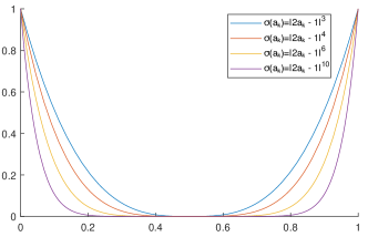
Figure 4: The proposed converting layer for converting the attention scores into confidence scores.

As shown in Fig. 2, in this confidence-based teacher-student fine-tuning method, we employ the trained aggregator in Classifier Phase to generate scores for the input instances. However, in MIL, attention scores often primarily emphasize positive instances and tend to disregard negative ones. Yet, for the embedder fine-tuning task, both positive and negative samples are required. Consequently, directly utilizing the attention score of each instance as its confidence score would result in a severe bias. To address this issue, we identify instances with high attention scores as high-confidence positive instances, and consider instances with extremely low attention scores as high-confidence negative samples. Therefore, we introduce a specialized converting layer $\sigma$ for the attention scores, as depicted in Fig. 4. This converting layer effectively projects the attention scores into confidence scores, which can be subsequently used to adjust the weights in the loss functions. The mathematical expression of the converting layer is:

$$\sigma(a_{k})=|2\cdot a_{k}-1|^{\beta},$$ (7)

where $a_{k}$ is the attention score for the $k$-th instance that ranges from 0 to 1 after min-max normalization, and $\beta$ is the hyper-parameter adjusting the smoothness of the converting function. $\beta$ is set to 6 by default in our experiments.

Altogether, the loss function for this confidence-based fine-tuning method is:

$$\mathscr{L}=\sigma(a(x))\cdot(\mathscr{L}_{c}+\alpha\mathscr{L}_{w}),$$ (8)

where $x$ is the input patch image as defined before, and $a(x)$ is its corresponding attention score generated by the aggregator.

4 Experiments

4.1 Datasets and Metrics

4.1.1 Datasets

There are four datasets used in our experiments. The first one is the widely used public benchmark Camelyon16 [30, 31, 32]. It consists of 270 training WSIs and provides an official test split with 129 cases. The positive WSIs in this dataset exhibit a severe class imbalance problem, with typically only about 10% tumor patches. Although detailed patch-level annotations are provided for this dataset, they are not used in our experiments but only used for visualization.

The second dataset is the public TCGA-Lung Dataset (i.e., TCGA Non-Small Cell Lung Carcinoma Dataset), which is composed of samples from the TCGA-LUAD (Lung Adenocarcinoma) project with 534 cases and the TCGA-LUSC (Lung Squamous Cell Carcinoma) project with 512 WSIs.

The third dataset is the public TCGA-RCC (Renal Cell Carcinoma) Dataset. This dataset contains three sub-type projects, namely Kidney Chromophobe Renal Cell Carcinoma (TGCA-KICH, 121 slides), Kidney Renal Clear Cell Carcinoma (TCGA-KIRC, 519 slides), and Kidney Renal Papillary Cell Carcinoma (TCGA-KIRP, 300 slides).

The last dataset is a private hepatocellular carcinoma (HCC) dataset collected from Sir Run Run Shaw Hospital, Hangzhou, China. This dataset comprises 1140 tumor WSIs scanned at 40$\times$ magnification. The task is to grade each case based on the Edmondson-Steiner (ES) grading scores. The ground truth labels are provided by experienced pathologists, where cases with ES grading I and II are labeled as low-risk cases, and cases with ES grading III and IV are considered as high-risk cases.

4.1.2 Metrics

For all the datasets, we evaluate the performance of different methods with three metrics, namely Area Under Curve (AUC), F1-score (F1), and Accuracy (Acc). The curve used for calculating AUC is the receiver operator characteristics (ROC) curve.

Table 1: Comparison between different embedder fine-tuning methods on Camelyon16 (w/o bag augmentation).

Backbone	Method	AUC (%)	F1 (%)	Acc (%)
Max Pooling	Naive Pseudo-label	84.0	73.5	80.8
	Vanilla ICMIL	85.2	74.4	81.9
	Confi-based ICMIL	85.2	74.4	81.9
ABMIL	Naive Pseudo-label	88.5	78.8	83.9
	Vanilla ICMIL	90.0	80.5	86.6
	Confi-based ICMIL	91.8	82.5	86.6
DTFD-MIL	Naive Pseudo-label	93.1	84.9	90.0
	Vanilla ICMIL	93.7	87.0	90.6
	Confi-based ICMIL	94.7	90.5	92.9

Table 2: Parameter study on $\beta$ of the converting layer for confidence-based ICMIL method (w/o bag augmentation).

Backbone of Confi-based ICMIL	Camelyon16				HCC
	$\beta$=2	$\beta$=4	$\beta$=6	$\beta$=8	$\beta$=2	$\beta$=4	$\beta$=6	$\beta$=8
ABMIL	90.9	91.3	91.8	91.7	87.3	87.9	87.9	87.4
DTFD-MIL	94.7	94.4	93.9	94.0	88.1	88.1	87.4	87.2

Table 3: Comparision of different bag-level augmentation strategies on Camelyon16 dataset with three different MIL backbones. The results are acquired with the confidence-based ICMIL method.

Method	Augmentation Method	Camelyon16			HCC			TCGA-Lung			TCGA-RCC
		AUC (%)	F1 (%)	Acc (%)	AUC (%)	F1 (%)	Acc (%)	AUC (%)	F1 (%)	Acc (%)	AUC (%)	F1 (%)	Acc (%)
Confidence- based ICMIL (w/ MaxPooling)	None	85.2	74.4	81.9	86.6	87.3	82.0	96.3	90.4	90.1	97.0	84.7	88.0
	Pseudo-bag	86.7	77.7	82.3	86.8	87.7	81.5	95.9	90.0	89.9	97.2	84.8	88.2
	Mix-up	87.0	78.8	83.1	86.6	88.0	82.1	96.3	90.7	90.7	97.2	84.5	88.3
	Both (Ours)	87.4	79.6	84.3	87.3	88.1	82.5	96.6	90.9	90.7	97.5	85.1	88.5
Confidence- based ICMIL (w/ ABMIL)	None	91.8	82.5	86.6	87.9	89.0	84.1	96.3	90.7	90.2	97.8	86.4	89.2
	Pseudo-bag	91.7	82.8	87.1	88.3	89.1	84.2	96.3	90.4	90.1	97.5	86.1	89.2
	Mix-up	92.2	83.7	87.4	88.5	89.0	83.9	95.3	90.0	89.7	97.9	86.1	88.9
	Both (Ours)	92.4	81.9	88.2	88.5	89.9	84.7	96.6	90.3	89.9	98.0	86.9	89.7
Confidence- based ICMIL (w/ DTFD-MIL)	None	94.7	90.5	92.9	88.1	89.7	84.0	97.2	91.4	91.3	97.6	88.4	89.8
	Pseudo-bag	94.1	90.0	92.2	88.0	89.5	83.6	96.3	90.4	90.1	97.1	88.1	89.5
	Mix-up	94.7	89.7	92.2	88.3	88.5	83.1	96.7	91.9	90.9	97.9	88.3	89.9
	Both (Ours)	95.0	88.2	91.3	88.9	90.2	84.5	96.8	91.9	91.3	97.9	88.6	90.2

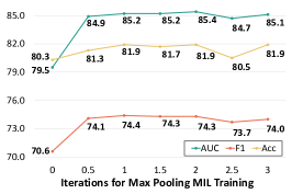
(a) Results w/ Max Pooling-based MIL

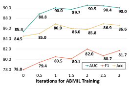
(b) Results w/ ABMIL

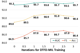
(c) Results w/ DTFD-MIL

Figure 5: AUC performance of ICMIL on Camelyon16 with different ceasing iterations for training.

4.2 Implementation Details

For the Camelyon16 and the two TCGA datasets, we tile the WSIs into non-overlapping patches of size 256$\times$256 at the 20$\times$ magnification level, following the same settings as the previous state-of-the-art method DTFD-MIL [22]. On the other hand, for the HCC dataset, we tile the WSIs into 384$\times$384 patches at the 40$\times$ magnification level based on the advice of pathologists. As a result, the Camelyon16 dataset yields approximately 3.7 million patches, the TCGA-Lung dataset generates around 15.3 million patches, the TCGA-RCC dataset generates around 12.9 million patches, and the HCC dataset produces approximately 17.4 million patches.

To comprehensively evaluate the proposed ICMIL method, we select three MIL approaches as the backbones for ICMIL, namely Max Pooling-based MIL, ABMIL, and the state-of-the-art method DTFD-MIL. During Classifier Phase, we utilize a learning rate of 2e-4 for the Adam optimizer [33] and train the MIL backbone for 200 epochs. For Embedder Phase, we use a learning rate of 1e-5 for the Adam optimizer [33], while the batch size is set to 80 for the HCC dataset and 100 for the others. The Camelyon16 results are reported on the official test split, while other datasets adopt a 7:1:2 split for training, validation, and testing. All experiments are implemented with PyTorch on a machine with two Xeon E5-2640 v4 CPUs, 96GB RAM, and an Nvidia Tesla M40 (12GB).

Table 4: Comparison with other methods on the four datasets. We use the confidence-based fine-tuning method to get the results, with $\beta$=2 for DTFD-MIL and $\beta$=6 for the others. The best results are in bold, while the second-best ones are underlined.

Method	Camelyon16			HCC			TCGA-Lung			TCGA-RCC
	AUC (%)	F1 (%)	Acc (%)	AUC (%)	F1 (%)	Acc (%)	AUC (%)	F1 (%)	Acc (%)	AUC (%)	F1 (%)	Acc (%)
Mean Pooling-based MIL	60.3	44.1	70.1	76.4	83.1	73.7	89.5	83.5	83.5	95.9	82.8	86.2
Max Pooling-based MIL	79.5	70.6	80.3	80.1	84.3	76.8	95.9	90.2	89.6	96.6	84.1	87.5
RNN-MIL [21]	87.5	79.8	84.4	79.4	84.1	75.5	89.4	83.1	84.5	96.2	83.1	86.6
ABMIL [18]	85.4	78.0	84.5	81.2	86.0	78.1	95.2	89.8	89.7	97.3	86.2	89.0
DSMIL [11]	89.9	81.5	85.6	86.1	86.6	81.4	93.9	87.6	88.8	97.2	85.0	88.9
CLAM-SB [17]	87.1	77.5	83.7	82.1	84.3	77.1	94.4	86.4	87.5	97.0	84.6	87.8
CLAM-MB [17]	87.8	77.4	82.3	81.7	83.7	76.3	94.9	87.4	87.8	97.5	87.1	89.5
TransMIL [19]	90.6	79.7	85.8	81.2	84.4	76.7	94.9	87.6	88.3	97.2	85.0	87.6
DTFD-MIL [22]	93.2	84.9	89.0	83.0	85.5	78.1	96.0	90.9	90.7	97.6	88.4	89.8
$\rm\mathop{Vanilla\ ICMIL}\limits_{(w/\ Max\ Pooling)}$ [16]	$\mathop{85.2}\limits_{(+5.7)}$	$\mathop{74.7}\limits_{(+4.1)}$	$\mathop{81.9}\limits_{(+1.6)}$	$\mathop{86.6}\limits_{(+6.5)}$	$\mathop{87.3}\limits_{(+3.0)}$	$\mathop{82.0}\limits_{(+5.2)}$	$\mathop{96.3}\limits_{(+0.4)}$	$\mathop{90.4}\limits_{(+0.2)}$	$\mathop{90.1}\limits_{(+0.5)}$	$\mathop{97.0}\limits_{(+0.4)}$	$\mathop{84.7}\limits_{(+0.6)}$	$\mathop{88.0}\limits_{(+0.5)}$
$\rm\mathop{Vanilla\ ICMIL}\limits_{(w/\ ABMIL)}$ [16]	$\mathop{90.0}\limits_{(+4.6)}$	$\mathop{80.5}\limits_{(+2.5)}$	$\mathop{86.6}\limits_{(+2.1)}$	$\mathop{87.1}\limits_{(+5.9)}$	$\mathop{88.3}\limits_{(+2.3)}$	$\mathop{83.3}\limits_{(+5.2)}$	$\mathop{95.9}\limits_{(+0.7)}$	$\mathop{90.4}\limits_{(+0.6)}$	$\mathop{90.0}\limits_{(+0.3)}$	$\mathop{97.6}\limits_{(+0.3)}$	$\mathop{86.5}\limits_{(+0.3)}$	$\mathop{89.1}\limits_{(+0.1)}$
$\rm\mathop{Vanilla\ ICMIL}\limits_{(w/\ DTFD\text{-}MIL)}$ [16]	$\mathop{93.7}\limits_{\underline{(+0.5)}}$	$\mathop{87.0}\limits_{\underline{(+2.1)}}$	$\mathop{90.6}\limits_{\underline{(+1.6)}}$	$\mathop{87.7}\limits_{(+4.7)}$	$\mathop{89.1}\limits_{(+3.6)}$	$\mathop{83.5}\limits_{(+5.4)}$	$\mathop{96.7}\limits_{\underline{(+0.7)}}$	$\mathop{91.1}\limits_{\underline{(+0.2)}}$	$\mathop{91.0}\limits_{\underline{(+0.3)}}$	$\mathop{97.7}\limits_{(+0.1)}$	$\mathop{88.4}\limits_{\underline{(+0.0)}}$	$\mathop{89.8}\limits_{\underline{(+0.0)}}$
$\rm\mathop{Confi\text{-}based\ ICMIL}\limits_{(w/\ Max\ Pooling)}$	$\mathop{87.4}\limits_{(+7.9)}$	$\mathop{79.6}\limits_{(+9.0)}$	$\mathop{84.3}\limits_{(+4.0)}$	$\mathop{87.3}\limits_{(+7.2)}$	$\mathop{88.1}\limits_{(+3.8)}$	$\mathop{82.5}\limits_{(+5.7)}$	$\mathop{96.6}\limits_{(+0.7)}$	$\mathop{90.9}\limits_{(+0.7)}$	$\mathop{90.7}\limits_{(+1.1)}$	$\mathop{97.5}\limits_{(+0.9)}$	$\mathop{85.1}\limits_{(+1.0)}$	$\mathop{88.5}\limits_{(+1.0)}$
$\rm\mathop{Confi\text{-}based\ ICMIL}\limits_{(w/\ ABMIL)}$	$\mathop{92.4}\limits_{(+7.0)}$	$\mathop{81.9}\limits_{(+3.9)}$	$\mathop{88.2}\limits_{(+3.7)}$	$\mathop{88.5}\limits_{\underline{(+7.4)}}$	$\mathop{89.9}\limits_{\underline{(+3.9)}}$	$\mathop{84.7}\limits_{\underline{(+6.6)}}$	$\mathop{96.6}\limits_{(+1.4)}$	$\mathop{90.3}\limits_{(+0.5)}$	$\mathop{89.9}\limits_{(+0.2)}$	$\boldsymbol{\mathop{98.0}\limits_{(+0.7)}}$	$\mathop{86.9}\limits_{(+0.7)}$	$\mathop{89.7}\limits_{(+0.7)}$
$\rm\mathop{Confi\text{-}based\ ICMIL}\limits_{(w/\ DTFD\text{-}MIL)}$	$\boldsymbol{\mathop{95.0}\limits_{(+1.8)}}$	$\boldsymbol{\mathop{88.2}\limits_{(+3.3)}}$	$\boldsymbol{\mathop{91.3}\limits_{(+2.3)}}$	$\boldsymbol{\mathop{88.9}\limits_{(+5.9)}}$	$\boldsymbol{\mathop{90.2}\limits_{(+4.7)}}$	$\boldsymbol{\mathop{84.5}\limits_{(+6.4)}}$	$\boldsymbol{\mathop{96.8}\limits_{(+0.8)}}$	$\boldsymbol{\mathop{91.9}\limits_{(+1.0)}}$	$\boldsymbol{\mathop{91.3}\limits_{(+0.6)}}$	$\mathop{97.9}\limits_{\underline{(+0.3)}}$	$\boldsymbol{\mathop{88.6}\limits_{(+0.2)}}$	$\boldsymbol{\mathop{90.2}\limits_{(+0.4)}}$

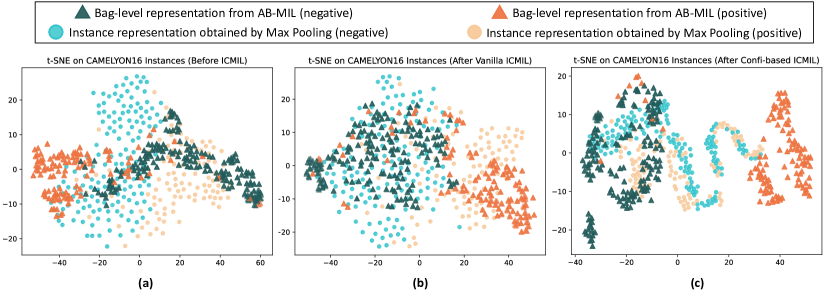
Figure 6: The t-SNE visualization results of bag-level representations from ABMIL and the instances sampled with Max Pooling on each bag. (a) Results before ICMIL. (b) Results after 1 iteration of vanilla teacher-student ICMIL. (c) Results after 1 iteration of confidence-based teacher-student ICMIL.

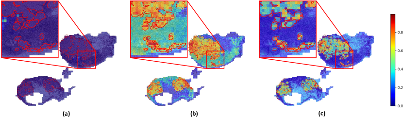
Figure 7: Visualization of the attention scores of the instances in a bag before and after ICMIL. Tested with ABMIL backbone on Camelyon16. The areas surrounded by the red lines are the ground truth tumor areas, while the colored masks of the patches indicate their corresponding attention scores. (a) The baseline ABMIL method, which tends to only highlight very few instances. (b) The vanilla ICMIL method, which can highlight the positive instance but struggles to mask the negative instances correctly. (c) The proposed confidence-based ICMIL method, which can not only highlight the positive instances but also correctly mask the negative instances.

4.3 Experimental Results

4.3.1 Ablation Study

To verify the effectiveness of the teacher-student fine-tuning method, we conducted an ablation study comparing different designs. Our comparison includes the naive pseudo-label-based method, the vanilla teacher-student method, and the proposed confidence-based teacher-student method. Specifically, the naive pseudo-label method refers to the approach that directly uses the bag classifier to generate pseudo-labels for all instances and then fine-tunes the embedder based on the generated instance dataset. The vanilla teacher-student method and the confidence-based method are described in Section 3.3.1 and Section 3.3.2, respectively.

The experimental results are presented in Table 1. From the table, we observe that although the naive pseudo-label method provides some improvement to the MIL pipeline by enabling domain-specific embedder fine-tuning, it fails to surpass the performance boost achieved by the other two teacher-student-based methods. This is because directly using pseudo-labels generated by the fixed embedder and classifier for fine-tuning the pipeline itself does not introduce enough additional information. In contrast, both teacher-student-based fine-tuning methods lead to more satisfactory results across all three backbones. Specifically, the confidence-based teacher-student method usually outperforms the vanilla method as it incorporates the attention scores from the MIL aggregator for fine-grained weighting. By incorporating the attention scores into the pipeline, more valuable information is highlighted during the fine-tuning, resulting in more effective learning.

Nevertheless, it should be noted that the confidence-based fine-tuning method can degrade to vanilla fine-tuning method for Max Pooling-based and Mean Pooling-based MIL methods, as they use non-learnable pooling layers as their aggregators, which generate one-hot or constant attention scores for all the instances. Using one-hot attention scores as the input for the converting layer will result in a constant 1 confidence score output, which is equivalent to not using the confidence-based scheme. Using constant attention scores (i.e., $\frac{1}{K}$) will lead to constant confidence scores. A constant confidence score for the instances will not affect the relative distribution of the training samples, making this confidence-based method still theoretically equivalent to the vanilla fine-tuning method.

4.3.2 Parameter Study about the Converting Layer

We further conduct a parameter study on $\beta$ of the converting layer. $\beta$ controls the number of uncertain instances that need to be masked during the confidence-based fine-tuning. As shown in TABLE 2, $\beta$=6 leads to the highest performance on ABMIL, while $\beta$=2 brings about the best results for DTFD-MIL. Generally speaking, the performance of ICMIL is not very sensitive to this parameter as long as it remains in a reasonable range. We empirically recommend using $\beta$=6 for most circumstances.

4.3.3 Comparison of Different Augmentation Methods

We have investigated different bag augmentation methods based on the three MIL backbones in our experiments, and the experimental results are presented in TABLE 3. From the table, we can learn that bag augmentation can bring performance improvement under most circumstances. When comparing the sole bag mix-up augmentation with the mix-up + pseudo-bag scheme, we can learn that the latter can usually outperform the former. This proves that the mix-up + pseudo-bag augmentation method can bring more diversity to the dataset, leading to better generalization ability of the model. For example, for Max Pooling-based MIL and ABMIL, mix-up + pseudo-bag augmentation lead to a remarkable boost in all three metrics on the Camelyon16 and HCC datasets.

4.3.4 Study on the Ceasing Point of Iteration

As an iterative optimization algorithm, determining the proper ceasing point for the iteration is vital. Therefore, we present an ablation study on Camelyon16 to find the most cost-effective creasing point for ICMIL. Each iteration involves one million patches for Embedder Phase. The experimental results of the performance based on different training iterations are presented in Fig. 5. From the graph, we can learn that the general performance of all three backbones tends to grow at the early iterations, and then become steady for the next few iterations. Although in certain cases some MIL backbones may achieve the highest AUC when trained with 2 ICMIL iterations, the extra performance boost is minor, especially when considering the extra training time. Therefore, we empirically recommend running ICMIL for one iteration.

4.3.5 Comparison with Other Methods

We also have a comprehensive comparison between existing MIL classification methods and ICMIL. The experimental results are presented in Table 4. As shown, confidence-based ICMIL that incorporates bag-level augmentation brings consistent improvements to the three backbones on all the datasets. Taking Camelyon16 as an example, ICMIL improves the AUC of Max Pooling-based MIL by 7.9% and ABMIL by 7.0%. When used with the current state-of-the-art MIL model DTFD-MIL, ICMIL further increases its performance by 1.8% AUC, 3.3% F1, and 2.3% Acc, demonstrating its effectiveness.

For the HCC dataset, the performance boost is also very obvious. Since risk grading is a more difficult task, the quality of the instance-level representations plays a crucial role in generating more separable bag-level representations. Therefore, after applying ICMIL, the three MIL backbones all gain great performance surge on the HCC dataset.

As to the two TCGA datasets, it is shown that the results of all the baseline MIL models are very high. Among them, Max Pooling-based MIL, ABMIL, and DTFD-MIL all achieved an AUC over 95%, leaving very little room for improvement. Nonetheless, ICMIL still bring consistent improvements to all three MIL backbones. On TCGA-Lung, for the state-of-the-art DTFD-MIL, ICMIL pushes its performance even further, leading to 96.8% AUC, 91.9% F1, and 91.3% Acc; On TCGA-RCC, ICMIL improves the performance of DTFD-MIL to 97.9% AUC, 88.6% F1, and 90.2% Acc.

4.3.6 Visualization Analysis

In Fig. 6, we present an intuitive comparison of the representations before and after ICMIL. Fig. 6(a) is the t-SNE visualization of the bag representations generated by ABMIL before ICMIL, with some instances sampled by Max Pooling from the bags in the background. It is shown that both the bag-level and the instance-level representations are somehow separable by two different boundaries. Fig. 6(b) presents the visualization results after 1 iteration of vanilla teacher-student embedder fine-tuning. As shown, the separability of the bag-level representations is improved. Besides, the bag representations also become more aligned with the instance representations, which is the natural result when using the bag-level decision boundaries to guide the instance-level embedder fine-tuning. However, when we change to use the proposed confidence-based embedder fine-tuning method, such alignment characteristics are weakened. This is because in this case, the fine-tuned representations from the embedder tend to be more tailored for the latent space of ABMIL, making the instance representations sampled by max pooling become less separable as shown in Fig. 6(c).

Additionally, in Fig. 7, we present a visual comparison of the highlighted instances in a bag before and after ICMIL. In Fig. 7(a), it is illustrated that the baseline ABMIL method tends to generate high attention scores only for a few distinctive instances. This is because it uses a frozen patch embedder and cannot project the WSI instances to an ideal subspace, in which case the aggregator tends to find the one single instance that can represent the entire bag. In comparison, as shown in Fig. 7(b), most of the tumor area patches are correctly highlighted after ICMIL. This indicates that the fine-tuned embedder finds a better latent space to project the positive and negative instances. However, it is also shown that many negative patches around the real tumor areas still receive incorrect high attention scores. In contrast, the proposed confidence-based ICMIL shows better performance as shown in Fig. 7(c). It can not only highlight the positive instances correctly, but also dim the negative patches properly. This proves the effectiveness of the confidence-based ICMIL.

5 Conclusion and Discussion

In this study, we have proposed the idea that a bag-level classifier can be a good instance-level teacher, and introduced ICMIL, a simple yet powerful framework for WSI classification. The primary objective of ICMIL is to bridge the gap between the patch embedding stage and the bag-level classification stage in existing MIL backbones. To address this challenge at a low cost, ICMIL proposes to couple the two stages in an iterative manner. To achieve an effective embedder fine-tuning process in Embedder Phase, we further propose a confidence-based teacher-student framework to facilitate category knowledge transfer from the bag classifier to the patch embedder. The extensive experiments on four different datasets using three representative MIL backbones demonstrate that ICMIL consistently enhances the performance of existing MIL backbones, achieving state-of-the-art results.

The limitations of the proposed confidence-based ICMIL mainly lie in that the converting layer used during the confidence score generation process is very simple and in certain cases it may require careful parameter tuning to avoid masking too many instances of uncertainty. In our future works, we will investigate and compare more different converting functions for the Embedder Phase and try to propose a self-adaptive converting layer for more accurate confidence score generation.

References

- [1] M. K. K. Niazi, A. V. Parwani, and M. N. Gurcan, “Digital pathology and artificial intelligence,” The lancet oncology, vol. 20, no. 5, pp. e253–e261, 2019.
- [2] M. Y. Lu, T. Y. Chen, D. F. Williamson, M. Zhao, M. Shady, J. Lipkova, and F. Mahmood, “Ai-based pathology predicts origins for cancers of unknown primary,” Nature, vol. 594, no. 7861, pp. 106–110, 2021.
- [3] Z. Su, T. E. Tavolara, G. Carreno-Galeano, S. J. Lee, M. N. Gurcan, and M. Niazi, “Attention2majority: Weak multiple instance learning for regenerative kidney grading on whole slide images,” Medical Image Analysis, vol. 79, p. 102462, 2022.
- [4] L. Hou, D. Samaras, T. M. Kurc, Y. Gao, J. E. Davis, and J. H. Saltz, “Patch-based convolutional neural network for whole slide tissue image classification,” in Proceedings of the IEEE conference on computer vision and pattern recognition, 2016, pp. 2424–2433.
- [5] C. Zhang, Y. Song, D. Zhang, S. Liu, M. Chen, and W. Cai, “Whole slide image classification via iterative patch labelling,” in 2018 25th IEEE International Conference on Image Processing (ICIP). IEEE, 2018, pp. 1408–1412.
- [6] Q. Chen, H. Xiao, Y. Gu, Z. Weng, L. Wei, B. Li, B. Liao, J. Li, J. Lin, M. Hei et al., “Deep learning for evaluation of microvascular invasion in hepatocellular carcinoma from tumor areas of histology images,” Hepatology International, vol. 16, no. 3, pp. 590–602, 2022.
- [7] H. R. Tizhoosh and L. Pantanowitz, “Artificial intelligence and digital pathology: challenges and opportunities,” Journal of pathology informatics, vol. 9, no. 1, p. 38, 2018.
- [8] O. Maron and T. Lozano-Pérez, “A framework for multiple-instance learning,” Advances in neural information processing systems, vol. 10, 1997.
- [9] O. Russakovsky, J. Deng, H. Su, J. Krause, S. Satheesh, S. Ma, Z. Huang, A. Karpathy, A. Khosla, M. Bernstein et al., “Imagenet large scale visual recognition challenge,” International journal of computer vision, vol. 115, no. 3, pp. 211–252, 2015.
- [10] C. L. Srinidhi, S. W. Kim, F.-D. Chen, and A. L. Martel, “Self-supervised driven consistency training for annotation efficient histopathology image analysis,” Medical Image Analysis, vol. 75, p. 102256, 2022.
- [11] B. Li, Y. Li, and K. W. Eliceiri, “Dual-stream multiple instance learning network for whole slide image classification with self-supervised contrastive learning,” in Proceedings of the IEEE/CVF conference on computer vision and pattern recognition, 2021, pp. 14 318–14 328.
- [12] R. J. Chen, C. Chen, Y. Li, T. Y. Chen, A. D. Trister, R. G. Krishnan, and F. Mahmood, “Scaling vision transformers to gigapixel images via hierarchical self-supervised learning,” in Proceedings of the IEEE/CVF Conference on Computer Vision and Pattern Recognition, 2022, pp. 16 144–16 155.
- [13] K. Liu, W. Zhu, Y. Shen, S. Liu, N. Razavian, K. J. Geras, and C. Fernandez-Granda, “Multiple instance learning via iterative self-paced supervised contrastive learning,” arXiv preprint arXiv:2210.09452, 2022.
- [14] X. Wang, F. Tang, H. Chen, L. Luo, Z. Tang, A.-R. Ran, C. Y. Cheung, and P.-A. Heng, “Ud-mil: uncertainty-driven deep multiple instance learning for oct image classification,” IEEE journal of biomedical and health informatics, vol. 24, no. 12, pp. 3431–3442, 2020.
- [15] C. Jin, Z. Guo, Y. Lin, L. Luo, and H. Chen, “Label-efficient deep learning in medical image analysis: Challenges and future directions,” arXiv preprint arXiv:2303.12484, 2023.
- [16] H. Wang, L. Luo, F. Wang, R. Tong, Y.-W. Chen, H. Hu, L. Lin, and H. Chen, “Iteratively coupled multiple instance learning from instance to bag classifier for whole slide image classification,” arXiv preprint arXiv:2303.15749, 2023.
- [17] M. Y. Lu, D. F. Williamson, T. Y. Chen, R. J. Chen, M. Barbieri, and F. Mahmood, “Data-efficient and weakly supervised computational pathology on whole-slide images,” Nature biomedical engineering, vol. 5, no. 6, pp. 555–570, 2021.
- [18] M. Ilse, J. Tomczak, and M. Welling, “Attention-based deep multiple instance learning,” in International conference on machine learning. PMLR, 2018, pp. 2127–2136.
- [19] Z. Shao, H. Bian, Y. Chen, Y. Wang, J. Zhang, X. Ji et al., “Transmil: Transformer based correlated multiple instance learning for whole slide image classification,” Advances in neural information processing systems, vol. 34, pp. 2136–2147, 2021.
- [20] A. Vaswani, N. Shazeer, N. Parmar, J. Uszkoreit, L. Jones, A. N. Gomez, Ł. Kaiser, and I. Polosukhin, “Attention is all you need,” Advances in neural information processing systems, vol. 30, 2017.
- [21] G. Campanella, M. G. Hanna, L. Geneslaw, A. Miraflor, V. Werneck Krauss Silva, K. J. Busam, E. Brogi, V. E. Reuter, D. S. Klimstra, and T. J. Fuchs, “Clinical-grade computational pathology using weakly supervised deep learning on whole slide images,” Nature medicine, vol. 25, no. 8, pp. 1301–1309, 2019.
- [22] H. Zhang, Y. Meng, Y. Zhao, Y. Qiao, X. Yang, S. E. Coupland, and Y. Zheng, “Dtfd-mil: Double-tier feature distillation multiple instance learning for histopathology whole slide image classification,” in Proceedings of the IEEE/CVF Conference on Computer Vision and Pattern Recognition, 2022, pp. 18 802–18 812.
- [23] T. Chen, S. Kornblith, M. Norouzi, and G. Hinton, “A simple framework for contrastive learning of visual representations,” in International conference on machine learning. PMLR, 2020, pp. 1597–1607.
- [24] Z. Luo, D. Guillory, B. Shi, W. Ke, F. Wan, T. Darrell, and H. Xu, “Weakly-supervised action localization with expectation-maximization multi-instance learning,” in Computer Vision–ECCV 2020: 16th European Conference, Glasgow, UK, August 23–28, 2020, Proceedings, Part XXIX 16. Springer, 2020, pp. 729–745.
- [25] Q. Wang, G. Chechik, C. Sun, and B. Shen, “Instance-level label propagation with multi-instance learning,” in Proceedings of the 26th International Joint Conference on Artificial Intelligence, 2017, pp. 2943–2949.
- [26] H. Zhang, M. Cisse, Y. N. Dauphin, and D. Lopez-Paz, “mixup: Beyond empirical risk minimization,” in International Conference on Learning Representations, 2018.
- [27] T. Asanomi, S. Matsuo, D. Suehiro, and R. Bise, “Mixbag: Bag-level data augmentation for learning from label proportions,” arXiv preprint arXiv:2308.08822, 2023.
- [28] P. Liu, L. Ji, X. Zhang, and F. Ye, “Pseudo-bag mixup augmentation for multiple instance learning based whole slide image classification,” arXiv preprint arXiv:2306.16180, 2023.
- [29] Q. Xie, M.-T. Luong, E. Hovy, and Q. V. Le, “Self-training with noisy student improves imagenet classification,” in Proceedings of the IEEE/CVF conference on computer vision and pattern recognition, 2020, pp. 10 687–10 698.
- [30] L. Luo, X. Wang, Y. Lin, X. Ma, A. Tan, R. Chan, V. Vardhanabhuti, W. C. Chu, K.-T. Cheng, and H. Chen, “Deep learning in breast cancer imaging: A decade of progress and future directions,” arXiv preprint arXiv:2304.06662, 2023.
- [31] C. Jin, Z. Guo, Y. Lin, L. Luo, and H. Chen, “Label-efficient deep learning in medical image analysis: Challenges and future directions,” arXiv preprint arXiv:2303.12484, 2023.
- [32] B. E. Bejnordi, M. Veta, P. J. Van Diest, B. Van Ginneken, N. Karssemeijer, G. Litjens, J. A. Van Der Laak, M. Hermsen, Q. F. Manson, M. Balkenhol et al., “Diagnostic assessment of deep learning algorithms for detection of lymph node metastases in women with breast cancer,” Jama, vol. 318, no. 22, pp. 2199–2210, 2017.
- [33] D. P. Kingma and J. Ba, “Adam: A method for stochastic optimization,” in International Conference on Learning Representations, 2015.