Minimal Model for Reservoir Computing

Abstract

A minimal model for reservoir computing is studied. We demonstrate that a reservoir computing exists that emulates given coupled maps by constructing a modularised network. We describe a possible mechanism for collapses of the emulation in the reservoir computing. Such transitory behaviour is caused by either (i) an escape from a finite-time stagnation near an unstable chaotic set, or (ii) a critical transition driven by the effective parameter drift. Our approach reveals the essential mechanism for reservoir computing and provides insights into the design of reservoir computing for practical applications.

1 Introduction

Machine learning, including the reservoir computing, has proven useful for model-free and data-driven predictions in a variety of scientific fields in recent years (see [1, 2] and references therein). In studies on nonlinear phenomena, the reservoir computing is typically applied to large-scale phenomena such as chemical reaction [3], fluid turbulence [4, 5], and climate and environmental dynamics [6, 7]. The purpose of the reservoir computing is to emulate the dynamics $u(t+1)=g(u(t))$ behind time-series data $\{u(t)\}$ using the dynamics $\{r(t)\}$ that is generated by a large recurrent neural network $r(t+1)=f_{A}(r(t))$ with a network matrix $A$ [8, 9, 10]. Assuming that $f_{A}$ approximates any continuous functions by tuning $A$ when a sufficiently large network is used [11], the trivial solution to this problem is $r(0)=u(0),~{}f_{A}\simeq g$.

As opposed to solving the non-convex optimisation problem to approximates $g$ with $f_{A}$ using a statistical optimisation method such as gradient descent, we may solve a simple convex optimisation problem using linear regression to obtain a projection of the network dynamics $P\{r(t)\}$, which is close to $\{u(t)\}$. The computation cost of the projection $P\{r(t)\}$ is clearly substantially smaller than that of the function approximation $f_{A}\simeq g$; however, we need to search for an appropriate initial network matrix $A$ for the successful emulation. The matrix $A$ is typically provided as a random matrix with a spectral radius $\rho(A)<1$ [8] (See Appendix A). One can search a number of the quenched random dynamics $\{r(t)\}$ by changing the random matrix $A$ to minimise $\lVert P\{r(t)\}-\{u(t)\}\rVert$. However, the design principle of such random matrices that satisfy appropriate quality, size, topology, and the order of the search cost is largely unknown.

As a statistical interpretation, it is pointed out that the reservoir computing is some kind of nonlinear regression [12]. Indeed, a reservoir computing performed by a neural network without hidden layers $f_{O}$ is a simple perceptron, that is equivalent to logistic regression. It is also known that random neural networks also approximate $C^{1}$ functions arbitrary well [13], which corresponds to the classical universal approximation theorem [11], and that the non-autonomous framework of reservoir computing is analogous to Takens’s embedding theorem, that works even under presence of noise [14, 15, 13]. See also Appendix B for the simplest example of a classical delay coordinate embedding performed by a non-autonomous reservoir computing.

In this study, instead of a Monte Carlo search for the network matrix $A$ and a validation of the quality of the reservoir computing with randomly selected $A$, we construct the smallest possible network that can be included in $A$ to emulate the given dynamical systems. We analyse the behaviour of the constructed dynamical systems, including transitory behaviour that induces the collapse of the emulation [16, 17]. Our approach reveals the essential mechanism for reservoir computing and provides insights into the design of reservoir computing for practical applications.

2 Reservoir Computing

We consider a reservoir computing at time $t$ with $M$-dimensional input neurons $\bm{x}(t)=(x^{(1)}(t),\ldots,x^{(M)}(t))^{T}$, output neurons $\bm{y}(t)=(y^{(1)}(t),\ldots,y^{(M)}(t))^{T}$, and a reservoir $\cal{A}$. The reservoir $\cal{A}$ includes $K$ hidden layer neurons $\bm{r}(t)=(r^{(1)}(t),\ldots,r^{(K)}(t))^{T}$, a $K\times K$ random matrix $A=(a_{ij})$ with a spectral radius $\rho(A)<1$, and an activation function $\sigma(\cdot)=\tanh(\cdot)$. The weights for the input and output are expressed as $W_{\rm{in}}=(w_{km})$ with $|w_{km}|<1$ and $W_{\rm{out}}=(v_{mk})$, where $m=1,\ldots,M,~{}k=1,\ldots,K$, respectively. The bias is given as $\bm{b}=(b_{k})$ with $(k=1,\ldots,K)$. We assume that the training data are generated using an $M$-dimensional continuous map $\bm{u}(t)=\bm{g}(\bm{u}(t))$.

In the non-autonomous training phase $t=-N,\ldots,0$, the entire system dynamics is determinied as follows:

$$\left\{\begin{array}[]{l}\bm{x}(t)=\bm{u}(t)\\ \bm{y}(t)=W_{\rm{out}}\bm{r}(t)~{}~{}~{}~{}~{}~{}~{}~{}~{}~{}~{}~{}~{}~{}~{}~{}~{}~{}~{}~{}~{}~{}~{}~{}~{}~{}(t=-N,\ldots,0)\\ r^{(k)}(t+1)=(1-\gamma)r^{(k)}(t)+\gamma\tanh\left[(A\bm{r}(t))_{k}+(W_{\rm{in}}\bm{x}(t))_{k}+b_{k}\right]\\ \end{array}\right.,$$ (1)

where $\gamma$ denotes the decay rate. At t=0, we minimise $\lVert\{\bm{y}(t)\}-\{\bm{u}(t)\}\rVert$ based on the generated $\{\bm{r}(t)\}$ to determine the optimal $W_{\rm{out}}=W_{\rm{out}}^{*}$. With a sufficiently large training data, linear regression is used to determine the optimal $W_{\rm{out}}^{*}$. At $t=0$, we replace $\bm{u}(t)$ with $\bm{y}(t)=W_{\rm{out}}^{*}\bm{r}(t)$, and express the system state as $\bm{x}(0)=\bm{u}(0)=\bm{y}(0)$.

In the autonomous prediction phase $t=1,2,\ldots$, we obtain

$$\left\{\begin{array}[]{l}\bm{x}(t)=\bm{y}(t)=W_{\rm{out}}^{*}\bm{r}(t)~{}~{}~{}~{}~{}~{}~{}~{}~{}~{}~{}~{}~{}~{}~{}~{}~{}~{}(t=1,2,\ldots)\\ r^{(k)}(t+1)=(1-\gamma)r^{(k)}(t)+\gamma\tanh\left[(A\bm{r}(t))_{k}+(W_{\rm{in}}\bm{y}(t))_{k}+b_{k}\right]\end{array}\right.,$$ (2)

and expect the emulation $\{\bm{u}(t)\}\simeq\{\bm{y}(t)\}$.

3 Emulating coupled maps

To construct a minimal example, we assume that the training data are generated by a class of one-dimensional maps given as

$$u(t+1)=(1-\gamma)u(t)+\gamma\sum_{k=1,2}v_{k}^{*}\tanh\left[\beta_{k}u(t)+\alpha_{k}\right].$$ (3)

Eq. (3) shows chaotic behaviour in a broad range of parameters. We adopt $\gamma=0.9,~{}~{}\beta_{1}=0.75,~{}~{}\beta_{2}=0.25,~{}~{}\alpha_{1}=\alpha_{2}=0,~{}~{}v^{*}_{1}=-12$, and $v_{2}^{*}=16$ as an example of a generator of chaotic training data. We emulate the dynamics of Eq. (3) using a reservoir $\cal{B}$ with $K=2$ (Fig. 1 (a)) to set

$$B=\begin{pmatrix}\mu_{1}v_{1}^{*}&\mu_{1}v_{2}^{*}\\ \mu_{2}v_{1}^{*}&\mu_{2}v_{2}^{*}\\ \end{pmatrix},~{}~{}0<\mu_{1},\mu_{2}\ll 1,~{}\rho(B)<1,$$ (4)

$$W_{\rm{in}}=\begin{bmatrix}\beta_{1}-\mu_{1}\\ \beta_{2}-\mu_{2}\\ \end{bmatrix},~{}~{}W_{\rm{out}}=\begin{bmatrix}v_{1}&v_{2}\\ \end{bmatrix},~{}~{}\bm{b}=\begin{bmatrix}\alpha_{1}\\ \alpha_{2}\\ \end{bmatrix}.$$ (5)

As $\mu_{1},\mu_{2}$ are free parameters, we may set $B$ satisfying the condition $\rho(B)<1$. Following linear regression with a sufficiently large training data $\{u(t)\}_{t=-N,\ldots,0}$, $W_{\rm{out}}$ is optimised to

$$W_{\rm{out}}^{*}=[v_{1}^{*}~{}v_{2}^{*}]$$ (6)

and we obtain

$$\left\{\begin{array}[]{l}x(t)=y(t)=v_{1}^{*}r^{(1)}(t)+v_{2}^{*}r^{(2)}(t)\\ r^{(1)}(t+1)=(1-\gamma)r^{(1)}(t)+\gamma\tanh\left[\beta_{1}y(t)+\alpha_{1}\right]\\ r^{(2)}(t+1)=(1-\gamma)r^{(2)}(t)+\gamma\tanh\left[\beta_{2}y(t)+\alpha_{2}\right]\\ \end{array}\right.,$$ (7)

resulting in

$$y(t+1)=(1-\gamma)y(t)+\gamma\sum_{k=1,2}v_{k}^{*}\tanh\left[\beta_{k}y(t)+\alpha_{k}\right],$$ (8)

which is equivalent to Eq. (3). Recall that at $t=0$ we obtain $x(0)=u(0)=y(0)$, and the dynamics is on $x=y=W_{\rm{out}}^{*}\bm{r}=v_{1}^{*}r^{(1)}+v_{2}^{*}r^{(2)}$, which may include the generalised synchronisation manifold in the reservoir $\cal{B}$ for the input $\{u(t)\}$ [18, 19]. Thus, we achieve a perfect emulation $\{y(t)\}=\{u(t)\}$ for $t=0,1,2,\ldots$ by using the $K=2$ reservoir $\cal{B}$. We confirm that the above emulation is achieved in numerical experiments with linear regression (Fig. 2 (a)). Many other possible constructions are available for given one-dimensional maps.

Next, we emulate a class of coupled maps, as follows:

$$\left\{\begin{array}[]{l}u^{(1)}(t+1)=(1-\epsilon)f(u^{(1)}(t))+\epsilon f(u^{(2)}(t))\\ u^{(2)}(t+1)=(1-\epsilon)f(u^{(2)}(t))+\epsilon f(u^{(1)}(t))\\ f(u)=(1-\gamma)u+\gamma\sum_{k=1,2}v_{k}^{*}\tanh\left[\beta_{k}u+\alpha_{k}\right]\\ \end{array}\right..$$ (9)

To emulate the dynamics of Eq. (9) using a reservoir $\cal{C}$ with $K=4$ (Fig. 1 (b)), we set

$$\begin{array}[]{l}C=\begin{pmatrix}\mu_{1}(1-\epsilon)v_{1}^{*}&\mu_{1}(1-\epsilon)v_{2}^{*}&\mu_{1}\epsilon v_{1}^{*}&\mu_{1}\epsilon v_{2}^{*}\\ \mu_{2}(1-\epsilon)v_{1}^{*}&\mu_{2}(1-\epsilon)v_{2}^{*}&\mu_{2}\epsilon v_{1}^{*}&\mu_{2}\epsilon v_{2}^{*}\\ \mu_{3}\epsilon v_{1}^{*}&\mu_{3}\epsilon v_{2}^{*}&\mu_{3}(1-\epsilon)v_{1}^{*}&\mu_{3}(1-\epsilon)v_{2}^{*}\\ \mu_{4}\epsilon v_{1}^{*}&\mu_{4}\epsilon v_{2}^{*}&\mu_{4}(1-\epsilon)v_{1}^{*}&\mu_{4}(1-\epsilon)v_{2}^{*}\\ \end{pmatrix},\\ \\ ~{}~{}~{}~{}~{}~{}~{}~{}~{}~{}0<\mu_{1},\mu_{2},\mu_{3},\mu_{4}\ll 1,~{}~{}\rho(C)<1\\ \end{array},$$ (10)

$$W_{\rm{in}}=\begin{bmatrix}\beta_{1}-\mu_{1}&0\\ \beta_{2}-\mu_{2}&0\\ 0&\beta_{1}-\mu_{3}\\ 0&\beta_{2}-\mu_{4}\\ \end{bmatrix},~{}~{}W_{\rm{out}}=\begin{bmatrix}v_{11}&v_{12}&v_{13}&v_{14}\\ v_{21}&v_{22}&v_{23}&v_{24}\\ \end{bmatrix},~{}~{}\bm{b}=\begin{bmatrix}\alpha_{1}\\ \alpha_{2}\\ \alpha_{1}\\ \alpha_{2}\\ \end{bmatrix}.$$ (11)

Following linear regression, $W_{\rm{our}}$ is optimised to

$$W_{\rm{out}}^{*}=\begin{bmatrix}(1-\epsilon)v_{1}^{*}&(1-\epsilon)v_{2}^{*}&\epsilon v_{1}^{*}&\epsilon v_{2}^{*}\\ \epsilon v_{1}^{*}&\epsilon v_{2}^{*}&(1-\epsilon)v_{1}^{*}&(1-\epsilon)v_{2}^{*}\\ \end{bmatrix},$$ (12)

and we obtain

$$\left\{\begin{array}[]{l}x^{(1)}(t)=y^{(1)}(t)=(W_{\rm{out}}^{*}\bm{r}(t))_{1}\\ x^{(2)}(t)=y^{(2)}(t)=(W_{\rm{out}}^{*}\bm{r}(t))_{2}\\ r^{(1)}(t+1)=(1-\gamma)r^{(1)}(t)+\gamma\tanh\left[\beta_{1}y^{(1)}(t)+\alpha_{1}\right]\\ r^{(2)}(t+1)=(1-\gamma)r^{(2)}(t)+\gamma\tanh\left[\beta_{2}y^{(1)}(t)+\alpha_{2}\right]\\ r^{(3)}(t+1)=(1-\gamma)r^{(3)}(t)+\gamma\tanh\left[\beta_{1}y^{(2)}(t)+\alpha_{1}\right]\\ r^{(4)}(t+1)=(1-\gamma)r^{(4)}(t)+\gamma\tanh\left[\beta_{2}y^{(2)}(t)+\alpha_{2}\right]\\ \end{array}\right.,$$ (13)

resulting in

$$\left\{\begin{array}[]{l}y^{(1)}(t+1)=(1-\epsilon)f(y^{(1)}(t))+\epsilon f(y^{(2)}(t))\\ y^{(2)}(t+1)=(1-\epsilon)f(y^{(2)}(t))+\epsilon f(y^{(1)}(t))\\ f(y)=(1-\gamma)y+\gamma\sum_{k=1,2}v_{k}^{*}\tanh\left[\beta_{k}y+\alpha_{k}\right]\\ \end{array}\right.,$$ (14)

which is equivalent to Eq. (9). Noting that $\bm{x}(0)=\bm{u}(0)=\bm{y}(0)$, and the dynamics is on $\bm{x}=\bm{y}=W_{\rm{out}}^{*}\bm{r}$, we achieve a perfect emulation $\{\bm{y}(t)\}=\{\bm{u}(t)\}$.

We confirm that the above emulation is achieved in numerical experiments with linear regression (Fig. 2 (b)). Many other possible constructions are available for given coupled maps.

Figure 1: (a) Model of $K=2$ reservoir for one-dimensional map, (b) model of $K=4$ reservoir for $2$-coupled maps, and (c) model of emulation collapse induced by excess neurons. The dotted circle indicates the collective excess neurons.

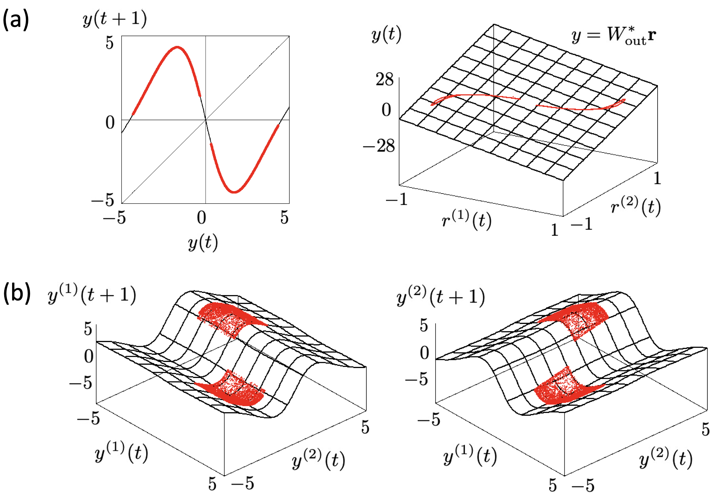
Figure 2: (a) Left:   map provided in Eq. (3) and return plots of $\{y(t)\}$ generated by constructed reservoir with $K=2$, and right:   attractor in $(r^{1)},r^{(2)},y)$, and the plane $y=W_{\rm{out}^{*}}\bm{r}$. (b) Map provided in Eq. (9) and return plots of $\{\bm{y}(t)\}$ generated by constructed reservoir with $K=4$. The parameters are $\gamma=0.9,~{}~{}\beta_{1}=0.75,~{}~{}\beta_{2}=0.25,~{}~{}\alpha_{1}=\alpha_{2}=0,~{}~{}v^{*}_{1}=-12,~{}~{}v_{2}^{*}=16,\epsilon=0.05$, and $\mu_{1}=\mu_{2}=\mu_{3}=\mu_{4}=0.01$.

In general, according to the property of neural networks as universal function approximators, we may emulate any one-dimensional maps

$$u(t+1)=(1-\gamma)u(t)+\gamma h(u(t)),$$ (15)

where $h$ denotes an arbitrary continuous functions. For a large $K$, the projected dynamics $\{y(t)\}$ of a reservoir with $K$ neurons can be expressed as follows:

$$\begin{array}[]{l}y(t+1)=(1-\gamma)y(t)+\gamma\sum_{k=1}^{K}v_{k}^{*}\tanh\left[\beta_{k}y(t)+\alpha_{k}\right]\\ ~{}~{}\stackrel{{\scriptstyle K\to\infty}}{{\longrightarrow}}~{}~{}y(t+1)=(1-\gamma)y(t)+\gamma h(y(t)).\\ \end{array}$$ (16)

For example, the projection $\{y(t)\}$ may emulate the logistic map $y(t+1)=a-y(t)^{2}$ when $h(y)\simeq-(1-\gamma)y+a-y^{2}$. Similarly, we can emulate arbitrary $M$-coupled maps with a linear coupling. To do that we use an $M$-dimensional projected dynamics of a reservoir with $KM$ neurons and a network matrix that consists of $M$ blocks of the size $K$. For example, with the construction in Eq. (9) where $f(y)\simeq a-y^{2}$, and the adequately optimised $W_{\rm{out}}^{*}$, the $M$-dimensional projected dynamics $\{\bm{y}(t)\}$ can emulate the dynamics of $M$-globally coupled logistic map $y^{(m)}(t+1)=(1-\epsilon)f(y^{(m)}(t))+\frac{\epsilon}{M}\sum_{i=1}^{M}f(y^{(i)}(t))$. This construction for coupled maps partially explains the successful emulation of PDEs by reservoir computing [16, 3]. Using a reservoir with a sufficiently large network, it is certainly possible to emulate the dynamics of a wide class of nonlinear PDEs, which are implemented on computers in the form of coupled maps. However, the essential problem is rather determining why a finite-size reservoir computing with a randomly selected network matrix efficiently emulates such dynamical systems with large degrees of freedom.

4 Emulation in large networks

Although the matrix $B$ or $C$ may be a part of a larger network matrix $A$, in certain cases in large networks, the system may degenerate and the effective dynamics may depend only on a smaller part of the network represented by $B$ or $C$. We consider such degeneration to the reservoir $\cal{B}$.

In general, some of neurons may not contribute to the emulation. We refer to a neuron with index $k$, where $w_{km}=v_{mk}=0$ holds for all $m$, as an ”excess neuron.” Assuming that $r^{(k)}~{}(k=3,\ldots,N)$ are excess neurons, and that their dynamics vanishes as $r^{(k)}\to 0$ when without the bias, the degeneration to the perfect emulation is achieved. We set a reservoir $\cal{A}$ with $K$ neurons, as follows:

$$A=\begin{pmatrix}B&R_{1}\\ O&R_{2}\\ \end{pmatrix},~{}~{}\rho(A)<1,$$ (17)

$$W_{\rm{in}}=\begin{bmatrix}\beta_{1}-\mu_{1}\\ \beta_{2}-\mu_{2}\\ 0\\ \vdots\\ 0\\ \end{bmatrix},~{}~{}W_{\rm{out}}=\begin{bmatrix}v_{1}\\ v_{2}\\ v_{3}\\ \vdots\\ v_{K}\\ \end{bmatrix}^{T},~{}~{}\bm{b}=\begin{bmatrix}\alpha_{1}\\ \alpha_{2}\\ 0\\ \vdots\\ 0\\ \end{bmatrix}.$$ (18)

When $R_{1}=O$ and $R_{2}$ is a random matrix, $W_{\rm{out}}$ is optimised to $W_{\rm{out}}^{*}=\begin{bmatrix}v_{1}^{*}&v_{2}^{*}&0&\cdots&0\\ \end{bmatrix}$, and Eq. (3) is emulated. In other cases, the projected dynamics $\{\bm{y}(t)\}$ may deviate from the perfect emulation by the perturbations from the collective excess neurons, which we discuss later in the paper.

The system may also degenerate by synchronisation of neurons. For example, we set a reservoir $\cal{D}$ as follows;

$$\begin{array}[]{l}D=\begin{pmatrix}\mu_{1}\frac{v_{1}^{*}}{2}&\mu_{1}\frac{v_{2}^{*}}{2}&\mu_{1}\frac{v_{1}^{*}}{2}&\mu_{1}\frac{v_{2}^{*}}{2}\\ \mu_{2}\frac{v_{1}^{*}}{2}&\mu_{2}\frac{v_{2}^{*}}{2}&\mu_{2}\frac{v_{1}^{*}}{2}&\mu_{2}\frac{v_{2}^{*}}{2}\\ \mu_{3}\frac{v_{1}^{*}}{2}&\mu_{3}\frac{v_{2}^{*}}{2}&\mu_{3}\frac{v_{1}^{*}}{2}&\mu_{3}\frac{v_{2}^{*}}{2}\\ \mu_{4}\frac{v_{1}^{*}}{2}&\mu_{4}\frac{v_{2}^{*}}{2}&\mu_{4}\frac{v_{1}^{*}}{2}&\mu_{4}\frac{v_{2}^{*}}{2}\\ \end{pmatrix},~{}~{}0<\mu_{1},\mu_{2},\mu_{3},\mu_{4}\ll 1,~{}\rho(D)<1\\ \end{array},$$ (19)

$$W_{\rm{in}}=\begin{bmatrix}\beta_{1}-\mu_{1}\\ \beta_{2}-\mu_{2}\\ \beta_{1}-\mu_{3}\\ \beta_{2}-\mu_{4}\\ \end{bmatrix},~{}~{}W_{\rm{out}}^{*}=\begin{bmatrix}v_{1}^{*}&v_{2}^{*}&v_{3}^{*}&v_{4}^{*}\\ \end{bmatrix},~{}~{}\bm{b}=\begin{bmatrix}\alpha_{1}\\ \alpha_{2}\\ \alpha_{1}\\ \alpha_{2}\\ \end{bmatrix}.$$ (20)

and obtain

$$\left\{\begin{array}[]{l}\bm{x}(t)=\bm{y}(t)=W_{\rm{out}}^{*}\bm{r}(t)\\ r^{(1)}(t+1)=(1-\gamma)r^{(1)}(t)+\gamma\tanh\left[\beta_{1}y(t)+\alpha_{1}\right]\\ r^{(2)}(t+1)=(1-\gamma)r^{(2)}(t)+\gamma\tanh\left[\beta_{2}y(t)+\alpha_{2}\right]\\ r^{(3)}(t+1)=(1-\gamma)r^{(3)}(t)+\gamma\tanh\left[\beta_{1}y(t)+\alpha_{1}\right]\\ r^{(4)}(t+1)=(1-\gamma)r^{(4)}(t)+\gamma\tanh\left[\beta_{2}y(t)+\alpha_{2}\right]\\ \end{array}\right..$$ (21)

The dynamics of $(r^{(3)},r^{(4)})$ in Eq. (21) is eventually synchronised to those of $(r^{(1)},r^{(2)})$ because

$$\left\{\begin{array}[]{l}r^{(1)}(t)-r^{(3)}(t)=(1-\gamma)(r^{(1)}(t)-r^{(3)}(t))\\ r^{(2)}(t)-r^{(4)}(t)=(1-\gamma)(r^{(2)}(t)-r^{(4)}(t))\end{array}\right..$$ (22)

As a result, the dynamics of $y(t)$ prefectly emulates Eq. (3). In large matrices, when the $K$-dimensional vector $\bm{r}$ is degenerated to a $2$-dimensional vector $(r^{(1)},r^{(2)})$ based on the synchronization to $2$ clusters $r^{(1)}=r^{(i)},r^{(2)}=r^{(j)},~{}(i\neq j,~{}3\leq i,j\leq K)$, again, the perfect emulation of Eq. (3) is achieved. Many other constructions are available for the degeneration by synchronisation.

While in gradient descent learning in multi-layer perceptrons, the degeneration of the network weights may cause vanishing gradient and decelerate learning [20, 21], the degeneration of the hidden layer dynamics in the reservoir computing may enhance precise emulations.

5 Collapse of emulation

When excess neurons exist, the dynamics $\{\bm{y}(t)\}$ in the subspace $\bm{x}=\bm{y}=W_{\rm{out}}^{*}\bm{r}$ can be perturbed, and the emulation may collapse in the long run. We create a model for the collapse of the emulation in Eq. (3) using a reservoir with $K=4$ and

$$\begin{array}[]{l}E=\begin{pmatrix}\mu_{1}v_{1}^{*}&\mu_{1}v_{2}^{*}&0&0\\ \mu_{2}v_{1}^{*}&\mu_{2}v_{2}^{*}&q_{1}&q_{2}\\ 0&0&\nu_{1}q_{1}&\nu_{1}q_{2}\\ 0&0&\nu_{2}q_{1}&\nu_{2}q_{2}\\ \end{pmatrix},~{}~{}0<\mu_{1},\mu_{2}\ll 1,~{}\rho(E)<1\\ \end{array},$$ (23)

$$W_{\rm{in}}=\begin{bmatrix}\beta_{1}-\mu_{1}\\ \beta_{2}-\mu_{2}\\ 0\\ 0\\ \end{bmatrix},~{}~{}W_{\rm{out}}^{*}=\begin{bmatrix}v_{1}^{*}&v_{2}^{*}&0&0\\ \end{bmatrix},~{}~{}\bm{b}=\begin{bmatrix}\alpha_{1}\\ \alpha_{2}\\ \alpha_{3}\\ \alpha_{4}\\ \end{bmatrix}.$$ (24)

For the entire system dynamics, we obtain

$$\left\{\begin{array}[]{l}x(t)=y(t)=v_{1}^{*}r^{(1)}(t)+v_{2}^{*}r^{(2)}(t)\\ \eta(t+1)=q_{1}r^{(3)}(t)+q_{2}r^{(4)}(t)\\ r^{(1)}(t+1)=(1-\gamma)r^{(1)}(t)+\gamma\tanh\left[\beta_{1}y(t)+\alpha_{1}\right]\\ r^{(2)}(t+1)=(1-\gamma)r^{(2)}(t)+\gamma\tanh\left[\beta_{2}y(t)+\alpha_{2}+\eta(t)\right]\\ r^{(3)}(t+1)=(1-\gamma)r^{(3)}(t)+\gamma\tanh\left[\nu_{1}\eta(t)+\alpha_{3}\right]\\ r^{(4)}(t+1)=(1-\gamma)r^{(4)}(t)+\gamma\tanh\left[\nu_{2}\eta(t)+\alpha_{4}\right]\\ \end{array}\right.,$$ (25)

$$\begin{array}[]{l}y(t+1)=(1-\gamma)y(t)+\gamma(v_{1}^{*}\tanh\left[\beta_{1}y(t)+\alpha_{1}\right]+v_{2}^{*}\tanh\left[\beta_{2}y(t)+\alpha_{2}+\eta(t))\right]\\ \end{array},$$ (26)

$$\eta(t+1)=(1-\gamma)\eta(t)+\gamma\sum_{k=1,2}q_{k}\tanh\left[\nu_{k}\eta(t)+\alpha_{k}\right].$$ (27)

When $\eta=0$, linear regression yields $W=W_{\rm{out}}^{*}$ and Eq. (26) is equivalent to Eq. (3). Thus, the collective excess neurons provides external perturbations to the projected dynamics $\{y(t)\}$. We present two examples of collapse of the emulation.

In the first example, we set $\gamma=0.9,q_{1}=-12,q_{2}=16,\nu_{1}=0.75$, and $\nu_{2}=0.5$ satisfying $\rho(E)<1$. When $\alpha_{3}=\tanh^{-1}(2/3)$ and $\alpha_{4}=\tanh^{-1}(1/2)$, Eq. (27) has a tangency at the origin and a stable fixed point $\eta=\eta^{*}\simeq 3.773341$. In this case, the perfect emulation can be performed as a neutral solution on the centre manifold $\eta=0$. The chaotic saddle is approached when we start at an initial point in the effective basin defined by $\eta(0)<0$ and $\eta(0)\notin(-2.197527,-0.985279)$; otherwise, the dynamics converges to $\eta=\eta^{*}$ and the linear regression fails. If we are not at the onset of the bifurcation point but very close to it with a narrow channel, the dynamics of $\eta(t)$ remains near the origin for a long time. If the waiting time near the origin, which typically follows a power law, is longer than the training time $N$, we start at $\eta(0)\simeq\eta^{*}$ at time $t=0$ and the projected dynamics $\{y(t)\}$ emulates $\{u(t)\}$ for a finite time. However, in the long run, the dynamics of $\{\eta(t)\}$ escapes from the narrow channel near the origin and converges to the stable fixed point $\eta=\eta^{*}$, and the emulation collapses (FIG 3 (a)).

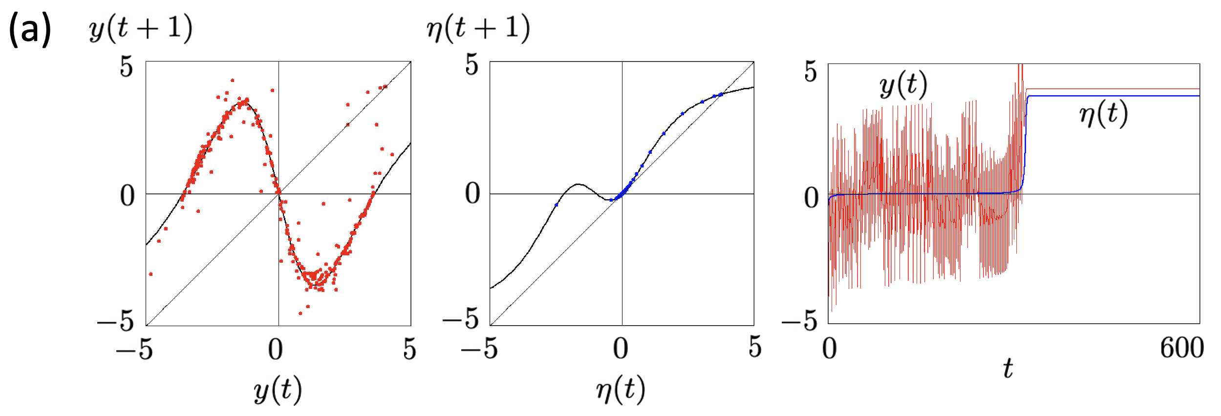
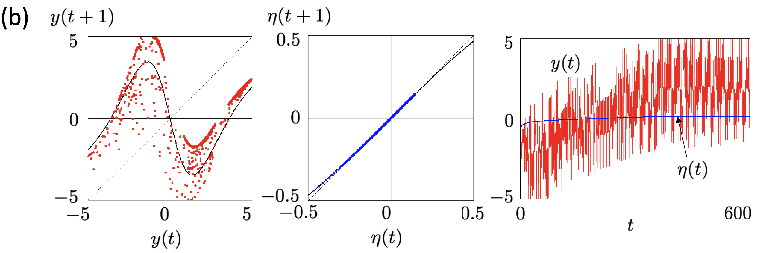
Figure 3: (a) Return plots and dynamics of the emulation collapse caused by a tangency. The parameters are $q_{1}=-12,q_{2}=16,\nu_{1}=0.75,\nu_{2}=0.5,\alpha_{3}=\tanh^{-1}(2/3)$, and $\alpha_{4}=\tanh^{-1}(1/2)$. The black line indicates Eqs. (26) and (27). The origin is neutrally stable and the fixed point $\eta=\eta^{*}\simeq 3.773341$ is stable in Eq. (27). (b) Return plots and dynamics of the emulation collapse caused by a critical transition. The parameters are $q_{1}=1,\nu_{1}=1-10^{-8}$, and $\alpha_{3}=0.001$. The black line indicates Eqs. (26) and (28). A narrow channel near the origin and a stable fixed point $\eta=\eta^{*}\simeq 0.143626$ exist.

The second example is based on only one excess neuron. We set $\gamma=0.9,q_{1}=1,\nu_{1}=1-10^{-8}$, and $\alpha_{3}=0.001$ satisfying $\rho(E)<1$ and obtain a hyperbolic tangent map

$$\eta(t+1)=(1-\gamma)\eta(t)+\gamma\tanh\left[\nu_{1}\eta(t)+\alpha_{3}\right].$$ (28)

In this case, the perfect emulation can be performed on an unstable chaotic set. The dynamics of Eq. (28) does not have tangencies but may have a narrow channel near the origin. It has a stable fixed point $\eta=\eta^{*}\simeq 0.143626$. The origin can be approached when we start at $\eta(0)<0$; otherwise, the dynamics converges to the stable fixed point $\eta=\eta^{*}$ and the linear regression fails. A very slow uniform motion $\eta(t)\simeq\gamma\tanh(\alpha_{3})t\simeq 10^{-4}t$ occurs near the origin, which functions as a parameter drift in Eq. (26). Thus, considering that other excess neurons function as external noise in a large network, bifurcation that is similar to the critical transition may occur [22, 17]. We observe orbits that are close to the training data for a finite time. However, before $\eta$ reaches to the stable fixed point $\eta=\eta^{*}$, it may arrive at the tipping point of Eq. (26) and the emulation collapses (FIG 3 (b)). In these two scenarios, the initial matrices and the initial conditions of $\bm{r}(0)$ have a positive measures in the parameter and state space. Thus, the above phenomena can be observed in a quenched random dynamical systems with a random matrix $A$ and with an initial condition $\bm{r}(0)$.

6 Conclusion

We have demonstrated that a reservoir computing exists that emulates given coupled maps by constructing a modularised network. We have proposed a possible mechanism for the collapses of the emulation in reservoir computing. Such transitory behaviour is caused by either (i) a finite-time stagnation near an unstable chaotic set or (ii) a critical transition by the effective parameter drift. The essential problem in reservoir computing is determining why a finite-size reservoir computing with a randomly selected network can efficiently emulate dynamical systems with large degrees of freedom. Our approaches provides a minimal model for understanding reservoir computing, thereby providing better insights into the design of reservoir computing for practical applications. Problems of quenched random dynamical systems analysis for bifurcations, generalised synchronisation, and collapse of the emulation will be studied elsewhere.

Acknowledgements We acknowledge H. Suetani for useful discussion and comments. The research leading to these results has been partially funded by the Grant in Aid for Scientific Research (B) No. 21H01002, JSPS, Japan, and the London Mathematical Laboratory External Fellowship, United Kingdom.

Appendix A Echo state property

The echo state property is a characteristic of a given reservoir dynamics with a network matrix $A$, where the reservoir dynamics converge to the same reservoir behavior as time tends to infinity, regardless of the choice of initial reservoir states [23]. As an empirical measure of the echo state property, the condition of the spectral radius of the network matrix $\rho(A)<1$ has been discussed. However, in our construction, we can set arbitrary spectral radii for perfect emulations of any coupled maps. In general, if multiple attractors exist, the echo state property does not hold [24].

Appendix B Delay coordinate embedding by reservoir computing

Assuming that the training data is provided as one-dimensional time series $\{u(t)\}$ and the attractor of the dynamics generating the training data $\bm{y}(t+1)=\bm{g}(\bm{y}(t))$ is a compact manifold of dimension $d$, the non-autonomous reservoir computing given by Eq. (1) with $2d+1$ output neurons, and with a smooth activation function is embedding by the embedding theorem [14, 15]. Both embedding and the reservoir computing unfold the training data into a high-dimensional space (or a reservoir), and take a projection of the high-dimensional structure. To see that with a simple example, we construct a $K=3$ reservoir computing $\cal{Q}$ with $1$-dimensional input neurons, $3$-dimensional output neurons, that embeds $1$-dimensional time series to $3$-dimensional state space. We assume that the training data are provided as $\{u(t)\}$ that is generated by a dynamical system whose effective dimension of stationary attractor is less than $3$. When the training data $\{u(t)\}$ is scaled to the dynamics very close to the origin, the activation function $\sigma(x)=\tanh(x)$ is an almost identical function as $\tanh(x)\simeq x~{}(x\simeq 0)$. We set $\gamma=1$, and

$$Q=\begin{pmatrix}0&0&0\\ 1&0&0\\ 0&1&0\\ \end{pmatrix},~{}~{}W_{\rm{in}}=\begin{bmatrix}1\\ 0\\ 0\\ \end{bmatrix},~{}~{}W_{\rm{out}}^{*}=\begin{bmatrix}1&0&0\\ 0&1&0\\ 0&0&1\\ \end{bmatrix},~{}~{}\bm{b}=\begin{bmatrix}0\\ 0\\ 0\\ \end{bmatrix},$$ (29)

and obtain

$$\left\{\begin{array}[]{l}x(t)=u(t)\\ \bm{y}(t)=W_{\rm{out}}^{*}\bm{r}(t)=\bm{r}(t)\\ r^{(1)}(t+1)=\tanh(x(t))\simeq x(t)\\ r^{(2)}(t+1)=\tanh(r^{(1)}(t))\simeq r^{(1)}(t)\\ r^{(3)}(t+1)=\tanh(r^{(2)}(t))\simeq r^{(2)}(t)\\ \end{array}\right..$$ (30)

Thus, $\bm{y}(t)$ is the classical delay coordinate embedding of the training data $\{u(t)\}$

$$\left\{\begin{array}[]{l}y^{(1)}(t+3)=r^{(1)}(t+3)\simeq x(t+2)=u(t+2)\\ y^{(2)}(t+3)=r^{(2)}(t+3)\simeq x(t+1)=u(t+1)\\ y^{(3)}(t+3)=r^{(3)}(t+3)\simeq x(t)=u(t)\\ \end{array}\right.$$ (31)

via a reservoir $\cal{Q}$. See [13] for the general embedding theorem for non-autonomous echo state networks.

References

• Lukoševičius and Jaeger [2009] M. Lukoševičius and H. Jaeger, Computer science review 3, 127 (2009).
• Tanaka et al. [2019] G. Tanaka, T. Yamane, J. B. Héroux, R. Nakane, N. Kanazawa, S. Takeda, H. Numata, D. Nakano, and A. Hirose, Neural Networks 115, 100 (2019).
• Pathak et al. [2018] J. Pathak, B. Hunt, M. Girvan, Z. Lu, and E. Ott, Physical review letters 120, 024102 (2018).
• Nakai and Saiki [2018] K. Nakai and Y. Saiki, Phys. Rev. E 98, 023111 (2018).
• Kobayashi et al. [2021] M. U. Kobayashi, K. Nakai, Y. Saiki, and N. Tsutsumi, Phys. Rev. E 104, 044215 (2021).
• Paulin [2010] C. Paulin, ournal of Hydrology 381, 76 (2010).
• Mitsui and Boers [2021] T. Mitsui and N. Boers, Environmental Research Letters 16, 074024 (2021).
• Jaeger [2001] H. Jaeger, GMD Report 148, 13 (2001).
• Jaeger and Haas [2004] H. Jaeger and H. Haas, Science 304, 78 (2004).
• Maass et al. [2002] W. Maass, T. Natschläger, and H. Markram, Neural Computation 14, 2531 (2002).
• Cybenko [1989] G. Cybenko, Mathematics of control, signals and systems 2, 303 (1989).
• Gauthier et al. [2021] D. J. Gauthier, E. Bollt, A. Griffith, and W. A. Barbosa, Nature communications 12, 5564 (2021).
• Hart et al. [2020] A. Hart, J. Hook, and J. Dawes, Neural Networks 128, 234 (2020).
• Takens [2006] F. Takens, in Dynamical Systems and Turbulence, Warwick 1980: proceedings of a symposium held at the University of Warwick 1979/80 (Springer, 2006), pp. 366–381.
• Sauer et al. [1991] T. Sauer, J. A. Yorke, and M. Casdagli, Journal of statistical Physics 65, 579 (1991).
• Pathak et al. [2017] J. Pathak, Z. Lu, B. R. Hunt, M. Girvan, and E. Ott, Chaos: An Interdisciplinary Journal of Nonlinear Science 27 (2017).
• Kong et al. [2021] L.-W. Kong, H.-W. Fan, C. Grebogi, and Y.-C. Lai, Physical Review Research 3, 013090 (2021).
• Lu et al. [2018] Z. Lu, B. R. Hunt, and E. Ott, Chaos: An Interdisciplinary Journal of Nonlinear Science 28 (2018).
• Lymburn et al. [2019] T. Lymburn, D. M. Walker, M. Small, and T. Jüngling, Chaos: An Interdisciplinary Journal of Nonlinear Science 29 (2019).
• Fukumizu and Amari [2000] K. Fukumizu and S.-I. Amari, Neural networks 13, 317 (2000).
• Sato et al. [2022] Y. Sato, D. Tsutsui, and A. Fujiwara, Physica D: Nonlinear Phenomena 430, 133095 (2022).
• Scheffer et al. [2009] M. Scheffer, J. Bascompte, W. A. Brock, V. Brovkin, S. R. Carpenter, V. Dakos, H. Held, E. H. Van Nes, M. Rietkerk, and G. Sugihara, Nature 461, 53 (2009).
• Yildiz et al. [2012] I. B. Yildiz, H. Jaeger, and S. J. Kiebel, Neural networks 35, 1 (2012).
• Ceni et al. [2020] A. Ceni, P. Ashwin, L. Livi, and C. Postlethwaite, Physica D: Nonlinear Phenomena 412, 132609 (2020).