Joint User Association and Resource Allocation for Multi-Cell Networks with Adaptive Semantic Communication

Abstract

Semantic communication is a promising communication paradigm that utilizes Deep Neural Networks (DNNs) to extract the information relevant to downstream tasks, hence significantly reducing the amount of transmitted data. In current practice, the semantic communication transmitter for a specific task is typically pre-trained and shared by all users. However, due to user heterogeneity, it is desirable to use different transmitters according to the available computational and communication resources of users. In this paper, we first show that it is possible to dynamically adjust the computational and communication overhead of DNN-based transmitters, thereby achieving adaptive semantic communication. After that, we investigate the user association and resource allocation problem in a multi-cell network where users are equipped with adaptive semantic communication transmitters. To solve this problem, we decompose it into three subproblems involving the scheduling of each user, the resource allocation of each base station (BS), and the user association between users and BSs. Then we solve each problem progressively based on the solution of the previous subproblem. The final algorithm can obtain near-optimal solutions in polynomial time. Numerical results show that our algorithm outperforms benchmarks under various situations.

I Introduction

It has been over seventy years since the inception of Shannon’s information theory [1]. During this period, traditional wireless communication technologies, aiming at the accurate transmission of bits, have made significant advancements and approached the Shannon limit. However, with the emergence of modern applications such as virtual reality and smart cities, the amount of data that needs to be transmitted continues to grow at an unprecedented pace. To meet the transmission demands with limited communication resources, a new communication paradigm called semantic communication has been proposed [2, 3, 4]. With the help of artificial intelligence technologies, semantic communication only transmits the information relevant to downstream tasks (which is usually referred to as semantic information), hence leading to a significant reduction in data traffic.

Although semantic communication can reduce the amount of transmitted data, extracting semantic information introduces additional computational overhead. In current practice, users performing the same task typically use the same semantic communication transmitter. However, due to the heterogeneity of users and networks, it is desirable to dynamically adjust the transmitter according to the available computational and communication resources. For example, since the transmitters are implemented by Deep Neural Networks (DNNs), we can decrease the model size of DNNs for users with limited computational capabilities. Similarly, for users with poor channel conditions, we can further reduce the amount of transmitted data by only transmitting a portion of the semantic information. By combining these two methods, we can obtain a range of semantic communication schemes with different computational overhead, communication overhead, and result accuracies. By selecting the optimal semantic communication scheme for each user, we can achieve adaptive semantic communication and significantly improve the system performance.

In this paper, we consider the joint user association and resource allocation problem for multi-cell networks with adaptive semantic communication. However, due to user heterogeneity (e.g. variations in computational capabilities, maximum transmitting power, and energy budget) and network heterogeneity (e.g. variations in user distribution, base station coverage, and channel conditions), there does not exist a straightforward solution for this problem. To solve this problem, we need to address the following challenges.

• Firstly, both computation and communication processes consume energy and time. Therefore, there exists a trade-off between the computational workload and the communication workload that a user can handle. Since the result accuracy depends on both kinds of workloads, we need to quantify this trade-off in order to obtain the optimal semantic communication scheme. However, how to quantify this trade-off is not explicitly clear.

• Secondly, in addition to transmitting power and transmission time, the spectrum bandwidth also influences the amount of transmitted data, thereby further affecting the result accuracy. However, due to user heterogeneity, the impact of spectrum bandwidth on result accuracy varies from user to user and hard to quantify. As a result, there is no simple rule to find the optimal spectrum allocation.

• Thirdly, due to network heterogeneity, associating all users with the nearest base station (BS) may result in severe load imbalance. Therefore, to make appropriate user association decisions, we need to consider both load balancing and channel conditions comprehensively. However, it is not clear how to measure the impact of these two factors.

To address the above challenges, this paper designs an efficient approximate algorithm to obtain near-optimal user association and resource allocation decisions in polynomial time. Our main contributions can be summarized as follows:

• We propose the concept of adaptive semantic communication and formulate the user association and resource allocation problem in a multi-cell network. We also show the formulated problem is strongly NP-hard.

• We progressively solve the problem by decomposing it into three subproblems involving the scheduling of each user, the resource allocation of each BS, and the user association between users and BSs. The solution to each subproblem relies on the properties of the optimal solution of the previous subproblem. The final algorithm can obtain near-optimal solutions in polynomial time.

• We conduct extensive simulations to evaluate the proposed algorithm under various settings. Numerical results demonstrate that our algorithm achieves significant improvement over benchmark algorithms.

The rest of the paper is organized as follows. In Section II, we review related works. In Section III, we describe the system model and formulate our optimization problem. Our algorithm design and theoretical analysis are presented in Section IV. In Section V, we show the numerical results to validate the performance of our algorithm. Section VI concludes the paper and discusses open problems for future work.

II Related Work

User association is an effective approach to balance the workload among multiple BSs, hence improve the overall system performance. In [5], the authors formulate the user association problem as an integer programming prolem and develop an efficient iterative algorithm by relaxing the integral constraints. However, the obtained solution allows users to associate with multiple BSs, which is usually not realistic in practice. The authors in [6] consider the user association problem in the context of massive multiple-input-multiple-output networks. The objective is to maximize the network utility by optimizing the fraction of time that a user associate with each BS. This problem is further extended to the case with cooperative BSs in [7]. Although user association is well studied in the conventional communication paradigm [8, 9, 10], these methods are not applicable in semantic communication because we also need to consider the influence of users’ computational capabilities on their transmission demands.

The concept of semantic communication has been proposed for a long time [11]. Recently, with the advancement of artificial intelligence technology, there has been a growing interest in utilizing DNNs to implement semantic communication. The authors in [12] designed a semantic communication framework for text transmission. Their approach is extended to construct semantic communication systems for other types of sources (e.g. image[13], speech[14], and video[15]), which has shown significant improvements over the conventional communication paradigm. To improve the performance of semantic communication systems, the authors in [16, 17, 18, 19, 20, 21] investigate the optimal resource allocation in various situations. However, they did not take into account the influence of users’ computational capabilities. Besides, most of these works only consider a single BS, which may lead to suboptimal result in ultra-dense networks.

III System Model and Problem Formulation

In this section, we first present the considered system and describe the concept of adaptive semantic communication. After that, we formulate an utility maximization problem and prove it is strongly NP-hard.

III-A Network Model

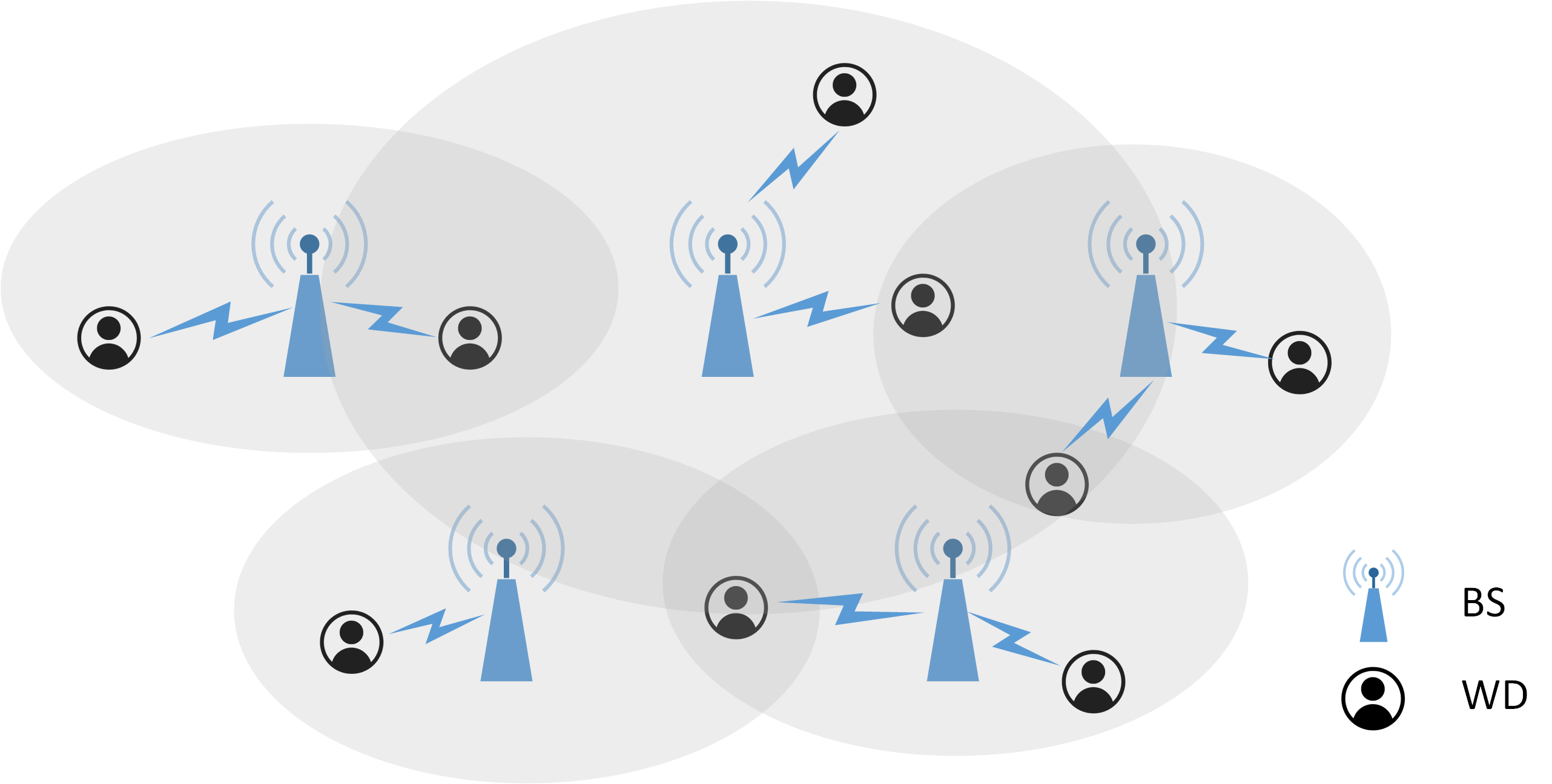
Figure 1: A simple example of the considered system.

As shown in Fig. 1, we consider a multi-cell network that consists of $M$ BSs and $N$ wireless devices (WDs), where one WD may communicate with multiple BSs. The set of all BSs and WDs are denoted by $\mathcal{M}$ and $\mathcal{N}$, respectively. There are a set $\mathcal{A}$ of $A$ applications running in the system. Let $\mathcal{N}_{a}\subseteq\mathcal{N}$ be the set of WDs belonging to application $a\in\mathcal{A}$. Each WD in $\mathcal{N}_{a}$ has a mount of raw data to be transmitted to BSs for further processing. For example, the WDs may be surveillance cameras that send captured photos to BSs for security risk detection. Due to limited wireless resources, the WDs will first extract the small-sized semantic information from the raw data (e.g. feature maps of the original photos) and only send the extracted semantic information to BSs.

In our considered model, a WD may be within the coverage of multiple BSs, so we need to determine which BS it communicates with. Specifically, the user association is denoted by the binary variable $x^{m}_{n}$, where $x^{m}_{n}=1$ if WD $n$ is associated with BS $m$, and $x^{m}_{n}=0$ otherwise. We assume a WD can communicate with at most one BS so $x^{m}_{n}$ should satisfy

$$\sum_{m\in\mathcal{M}}x^{m}_{n}\leq 1,\quad\forall n\in\mathcal{N}.$$ (1)

III-B Adaptive Semantic Communication Model

In existing semantic communication works, it is commonly assumed that the same transmitter is shared by all WDs. However, due to user heterogeneity, different WDs may prefer different semantic communication schemes. For example, if a WD has weak computational power but good channel conditions and rich spectrum resources, it may transmit the raw data to the BS without extracting the semantic information. In contrast, if a WD has strong computational power but limited communication resources, it can fully process the raw data and only send the final computation results to the BS. Therefore, by choosing appropriate semantic communication schemes, we can optimize the utilization of communication and computational resources, thereby enhancing system performance.

In practice, there are several ways to generate different semantic communication schemes. For example, the works in [22, 23, 24, 25] proposed various techniques to train DNNs of different model sizes in a single training process. Smaller models require less computation but also have worse accuracy. Since the semantic transmitters are implemented by DNNs, we can use these techniques to obtain a series of transmitters to achieve efficiency-accuracy trade-offs. Another method to derive multiple semantic communication schemes is through semantic compression [18, 19, 20, 21]. The basic idea is, after extracting the semantic information, the transmitter evaluates the importance of each component of the extracted semantic information and only transmit those that contribute most to the result accuracy. The evaluation of semantic information induces extra computation but the amount of data to be transmitted can be significantly reduced.

According to the above discussion, for a given application $a$, its result accuracy is determined by the computation workload $c^{a}$ (defined as the number of CPU cycles required to extract the semantic information) and the communication workload $d^{a}$ (defined as the amount of data to be transmitted). Therefore, we can use the utility function $u^{a}(c,d)$ to represent the obtained utility when the computation and communication workload is $c$ and $d$. It is worth noting that in practice, $c$ and $d$ are often limited to discrete values. For example, in semantic compression, each component of the semantic information cannot be further divided so $d$ must be an integer multiple of the data size of each component. However, the possible values of $c$ and $d$ are usually relatively dense so $u^{a}(c,d)$ can be regarded as a sufficiently good approximation.

III-C Computation and Transmission Model

In current practice, semantic information extraction is usually performed by DNNs, which requires a large amount of computation. For energy efficiency considerations, we assume WDs adopt the Dynamic Voltage and Frequency Scaling (DVFS) technique [26] to dynamically adjust the CPU frequency. For WD $n\in\mathcal{N}_{a}$, let $f_{n}$ be its CPU frequency and $c_{n}$ be its computation workload, then the computation time for semantic information extraction is

$$T^{c}_{n}=\frac{c_{n}}{f_{n}}.$$ (2)

According to the results in [27], the energy consumption per CPU cycle is proportional to the square of the frequency, which can be expressed as $\gamma_{n}f^{2}_{n}$, where $\gamma_{n}$ is the energy-efficiency factor determined by the chip architecture. Hence, the energy consumption due to computation is

$$E^{c}_{n}=c_{n}\gamma_{n}f^{2}_{n}.$$ (3)

The spectrum bandwidth of each BS is equally divided into resource blocks (RBs) with bandwidth $W$ and the number of available RBs at BS $m$ is $K_{m}$. Let $z^{m}_{n}\in\{0,1,\dots,K_{m}\}$ be the number of BS $m$’s RBs allocated to WD $n$. As in [28, 29, 30, 31], we assume the inter-BS interference is randomized and/or mitigated by various coordination techniques so the total interference seen by each BS can be regarded as static. According to the Shannon capacity formula, the transmission rate from WD $n$ to BS $m$ can be expressed as:

$$r^{m}_{n}=z^{m}_{n}W\log_{2}\left(1+\frac{P_{n}h^{m}_{n}}{\sigma^{2}+I_{m}}\right),$$ (4)

where $P_{n}$ is the transmission power of WD $n$, $h^{m}_{n}$ is the channel gain between WD $n$ and BS $m$, $\sigma^{2}$ is the noise power at BS $m$, and $I_{m}$ is the average interference seen by BS $m$. Clearly, for each BS $m$, the number of totally allocated RBs cannot exceed $K_{m}$, so we have

$$\sum_{n\in\mathcal{N}}z^{m}_{n}\leq K_{m},\quad\forall m\in\mathcal{M}.$$ (5)

For WD $n\in\mathcal{N}_{a}$, let $d_{n}$ be the amount of data to be transmitted, then the transmission time is

$$T^{t}_{n}=\frac{d_{n}}{\sum_{m\in\mathcal{M}}x^{m}_{n}r^{m}_{n}}$$ (6)

and the energy consumption due to transmission is

$$E^{t}_{n}=P_{n}T^{t}_{n}.$$ (7)

III-D Problem Formulation

In this paper, we aim to maximize the total utility by jointly optimizing the user association and resource allocation under energy consumption, wireless bandwidth, and completion time constraints. Based on the models described above, the corresponding optimization problem can be formulated as follows:

$$\max_{\begin{subarray}{c}\bm{x},\bm{z},\bm{f},\bm{P}\\ \bm{c},\bm{d}\end{subarray}}\quad \sum_{a\in\mathcal{A}}\sum_{n\in\mathcal{N}_{a}}u^{a}(c_{n},d_{n})$$ (8)

$$s.t.\quad \eqref{cons:association}\mbox{ and }\eqref{cons:RB}\quad$$ (8a)

$$T^{c}_{n}+T^{t}_{n}\leq T^{max},\quad\forall n\in\mathcal{N}$$ (8b)

$$E^{c}_{n}+E^{t}_{n}\leq E^{max}_{n},\quad\forall n\in\mathcal{N}$$ (8c)

$$0\leq f_{n}\leq f^{max}_{n},\quad\forall n\in\mathcal{N}$$ (8d)

$$0\leq P_{n}\leq P^{max}_{n},\quad\forall n\in\mathcal{N}$$ (8e)

$$x^{m}_{n}\in\{0,1\},\quad\forall m\in\mathcal{M},\forall n\in\mathcal{N}$$ (8f)

$$z^{m}_{n}\in\{0,1,\dots,K_{m}\},\quad\forall m\in\mathcal{M},\forall n\in\mathcal{N}$$ (8g)

where $\bm{x},\bm{z},\bm{f},\bm{P},\bm{c},\bm{d}$ are vetors of corresponding decision variables. Constraint (8a) contains the user association and RB allocation constraints described above. Constraint (8b) ensures the semantic information transmission is completed before the maximum delay $T^{max}$. Constraint (8c) requires the total energy consumption of WD $n$ does not exceed a given threshold $E^{max}_{n}$. Constraints (8d), (8e), (8f), and (8g) define the ranges of feasible values for the decisions variables, where $f^{max}_{n}$ and $P^{max}_{n}$ are the maximum CPU frequency and transmission power of WD $n$, respectively.

The formulated problem is Mixed-Integer Programming (MIP) and can be hard to solve. Specifically, we will show that our problem is strongly NP-hard, so it does not even have a pseudo-polynomial time algorithm. Before stating our result, we give the definition of binary utility functions: we say an utility function $u^{a}(c,d)$ is binary if $u^{a}(c,d)=u^{a}_{0}$ for all $(c,d)\geq(c^{a}_{0},d^{a}_{0})$ and $u^{a}(c,d)=0$ otherwise, where $u^{a}_{0},c^{a}_{0},d^{a}_{0}$ are positive constants.

Theorem 1.

Problem (8) is strongly NP-hard even if (i) there is only one WD for each running application and its utility function is binary, (ii) the energy budget $E^{max}_{n}$ is sufficiently large, and (iii) the channel gain $h^{m}_{n}$ and interference $I_{m}$ for different BS $m$ is equal.

Proof.

Please see Appendix A. ∎

Thereom 1 indicates that problem (8) is hard to solve even for a significantly simplified case. Therefore, in general, it is computationally intractable to obtain the exact solution of problem (8). In the next section, we will design an approximate algorithm that produces near-optimal solutions for problem (8) in polynomial time.

IV Algorithm Design and Performance Analysis

In this section, we will progressively solve the formulated problem through three stages. Firstly, we find the optimal scheduling decisions $\bm{f},\bm{P},\bm{c},\bm{d}$ when the user association and RB allocation are given. Based on this result, we can solve the optimal RB allocation under any user association. Finally, we can obtain the optimal user association by employing a relaxation-then-refinement approach.

IV-A Scheduling Subproblem for Each WD

If the user association $\bm{x}$ and RB allocation $\bm{z}$ are given, problem (8) can be decomposed into $N$ subproblems concerning the scheduling of each WD. Specifically, for any WD $n\in\mathcal{N}_{a}$ associated with BS $m$, its scheduling subproblem can be formulated as:

$$\max_{{f_{n}},{P_{n}},c_{n},d_{n}}\quad u^{a}(c_{n},d_{n})$$ (9)

$$s.t.\quad T^{c}_{n}+T^{t}_{n}\leq T^{max},$$ (9a)

$$E^{c}_{n}+E^{t}_{n}\leq E^{max}_{n},$$ (9b)

$$0\leq f_{n}\leq f^{max}_{n},0\leq P_{n}\leq P^{max}_{n}$$ (9c)

We say a computation and communication workload pair $(c_{n},d_{n})$ is achievable if there exists $f_{n},P_{n}$ such that constraints (9a)-(9c) are satisfied. The set of all achievable workload pairs is referred to as the achievable region. Since $u^{a}(c_{n},d_{n})$ is non-decreasing, the optimal workload pair $(c^{*}_{n},d^{*}_{n})$ must lie on the boundary of the achievable region, i.e. there is no achievable $(c_{n},d_{n})$ such that $c_{n}=c^{*}_{n}$ and $d_{n}>d^{*}_{n}$. To obtain the achievable region, we only need to calculate the maximum achievable $d_{n}$ for any given $c_{n}$, denoted by $d^{max}_{n}(c_{n})$. The calculation of $d^{max}_{n}(c_{n})$ can be formulated as another optimization problem

$$\max_{f_{n},P_{n}}\quad d_{n}$$ (10)

$$s.t.\quad \eqref{sub:cons:delay}-\eqref{sub:cons:fp}.$$

To solve problem (10), we first show that its optimal solution satisfies the following condition.

Theorem 2.

The optimal solution $(f^{*}_{n},P^{*}_{n})$ of problem (10) must satisfy

$$T^{c}_{n}+T^{t}_{n} =T^{max}$$ (11)

$$E^{c}_{n}+E^{t}_{n} =E^{max}_{n}.$$ (12)

Proof.

Please see Appendix B. ∎

According to Theorem 2, we can replace constraint (9a) and (9b) with (11) and (12). Substituting (2) and (6) into (11) and recalling that WD $n$ is associated with BS $m$ (i.e. $x^{m}_{n}=1$) result in

$$P_{n}=\left(2^{\frac{d_{n}f_{n}}{(f_{n}T^{max}-c_{n})z^{m}_{n}W}}-1\right)\frac{\sigma^{2}+I_{m}}{h^{m}_{n}}.$$ (13)

Combining (13) with (9c) we get the feasible region of $f_{n}$:

$$\frac{z^{m}_{n}Wc_{n}\log_{2}\left(1+\frac{P_{n}^{max}h^{m}_{n}}{\sigma^{2}+I_{m}}\right)}{z^{m}_{n}WT^{max}\log_{2}\left(1+\frac{P_{n}^{max}h^{m}_{n}}{\sigma^{2}+I_{m}}\right)-d_{n}}\leq f_{n}\leq f_{n}^{max}.$$ (14)

Substituting (3), (7) and (13) into (12) yields

$$d_{n}= z^{m}_{n}W\left(T^{max}-\frac{c_{n}}{f_{n}}\right)\times$$

$$\quad\log_{2}\left(1+\frac{h^{m}_{n}(E^{max}-c_{n}\gamma_{n}f^{2}_{n})}{(T^{max}-\frac{c_{n}}{f_{n}})(\sigma^{2}+I_{m})}\right).$$ (15)

Hence, problem (10) is equivalent to finding the optimal $f_{n}$ that maximizes (15) subject to (14), which can be solved by letting $\frac{\partial d_{n}}{\partial f_{n}}=0$ and comparing the values of $d_{n}$ achieved by every critical point in the feasible region. Clearly, the optimal $f_{n}$ is a function of $c_{n}$, denoted by $f^{*}_{n}(c_{n})$. According to (15), we can regard $d_{n}$ as a function of $c_{n}$ and $f_{n}$. Then we have $d^{max}_{n}(c_{n})=\max_{f_{n}}d_{n}(c_{n},f_{n})=d_{n}(c_{n},f^{*}_{n}(c_{n}))$. Unfortunately, the expression of $\frac{\partial d_{n}}{\partial f_{n}}=0$ is fairly complex so we are unable to derive an analytical expression for $f^{*}_{n}(c_{n})$. However, we can still calculate the value of $f^{*}_{n}(c_{n})$ through numerical methods.

Once we know how to calculate $d^{max}_{n}(c_{n})$, problem (9) is equivalent to $\max_{c_{n}}u^{a}(c_{n},d^{max}_{n}(c_{n}))$. Similarly, the optimal $c_{n}$ can be obtained by letting

$$\frac{\mathop{}\!\mathrm{d}u^{a}(c_{n},d^{max}_{n}(c_{n}))}{\mathop{}\!\mathrm{d}c_{n}}$$

$$\quad=\frac{\partial u^{a}}{\partial c_{n}}+\frac{\partial u^{a}}{\partial d^{max}_{n}}\times\frac{\mathop{}\!\mathrm{d}d^{max}_{n}}{\mathop{}\!\mathrm{d}c_{n}}$$

$$\quad=\frac{\partial u^{a}}{\partial c_{n}}+\frac{\partial u^{a}}{\partial d^{max}_{n}}\times\left(\frac{\partial d_{n}}{\partial c_{n}}+\frac{\partial d_{n}}{\partial f^{*}_{n}}\times\frac{\mathop{}\!\mathrm{d}f^{*}_{n}}{\mathop{}\!\mathrm{d}c_{n}}\right)$$

$$\quad=\frac{\partial u^{a}}{\partial c_{n}}+\frac{\partial u^{a}}{\partial d^{max}_{n}}\times\frac{\partial d_{n}}{\partial c_{n}}=0$$

where the second equality holds because $d^{max}_{n}(c_{n})=d_{n}(c_{n},f^{*}_{n}(c_{n}))$ and the third equality holds because $\frac{\partial d_{n}}{\partial f^{*}_{n}}=0$. Similarly, the optimal $c_{n}$ can only be solved by numerical methods. After obtaining the optimal $c_{n}$, the optimal values of the rest decision variables can be calculated easily.

IV-B RB Allocation Subproblem for Each BS

In the previous subsection, we have obtained the optimal $\bm{f},\bm{P},\bm{c},\bm{d}$ for any given $\bm{x}$ and $\bm{z}$. In this subsection, we still assume $\bm{x}$ is given and show how to find the optimal $\bm{z}$. Let $u^{*}_{n}(z^{m}_{n})$ be the optimal objective value of problem (9). The meaning of $u^{*}_{n}(z^{m}_{n})$ is the maximum achievable utility of WD $n$ when $z^{m}_{n}$ RBs are allocated to it. Since $\bm{x}$ is given, we can use $\mathcal{N}_{m}$ to denote the set of WDs associated with BS $m$. Then the RB allocation subproblem for BS $m$ becomes

$$\max_{z^{m}_{n}}\quad \sum_{n\in\mathcal{N}_{m}}u^{*}_{n}(z^{m}_{n})$$ (16)

$$s.t.\quad \sum_{n\in\mathcal{N}_{m}}z^{m}_{n}\leq K_{m},$$ (16a)

$$z^{m}_{n}\in\{0,1,\dots,K_{m}\},\quad\forall n\in\mathcal{N}_{m}.$$ (16b)

In this subsection, we will design two different algorithms for problem (16) based on the properties of the utility function $u^{a}(c,d)$. In practice, the most commonly used utility function is the result accuracy, e.g. the classification accuracy in image recognition tasks. In this case, the utility function usually exhibits concavity and other properties that can be exploited to accelerate the solving of problem (16). However, in some scenarios, we may encounter more general utility functions. Therefore, we also design an algorithm that does not require the concavity of the utility function.

IV-B1 RB Allocation with Concave Utility

If the utility function is the result accuracy or a concave function of the result accuracy, then it should satisfy the following three properties. Firstly, according to the results in [22, 23, 24, 25, 18, 19, 20, 21], the marginal return of $c$ and $d$ is diminishing. Hence, we can assume:

Assumption 1.

$u^{a}(c,d)$ is non-descreasing and concave.

Secondly, the marginal return of computation workload should be non-decreasing with respect to the amount of transmitted data. This is because the improvement in result accuracy due to increased computation needs to be propagated to the destination through data transmission. If the amount of transmitted data is limited, then the enhancement obtained at the destination will be discounted. An extreme example is the marginal return of $c$ is $0$ when $d=0$, as $u^{a}(c,0)=0$ for all $c$. Therefore, we have:

Assumption 2.

$\frac{\partial u^{a}}{\partial c}$ is non-decreasing with respect to $d$.

Thirdly, according to the results in [19], the marginal return of $d$ drops rapidly, which means the partial derivative of $u^{a}(c,d)$ with respect to $d$ also decreases rapidly. Hence, we can assume $\frac{\partial u^{a}}{\partial d}$ satisfies the following property:

Assumption 3.

$\frac{\partial u^{a}}{\partial d}|_{(c,\alpha d)}\leq\frac{1}{\alpha}\frac{\partial u^{a}}{\partial d}|_{(c,d)}$ for any $\alpha\geq 1$.

Assumption 3 requires $\frac{\partial u^{a}}{\partial d}$ decreases at least at a linear rate of $d$. A common function that satisfies this assumption is the logarithmic function. In practice, this assumption generally does not hold strictly, but it can be regarded as approximately valid within the range of values that we are interested in.

With the above assumptions, we can proceed to demonstrate the concavity of $u^{*}_{n}(z^{m}_{n})$. However, $z^{m}_{n}$ is a discrete variable and the concavity for discrete functions is not well-defined. Therefore, we relax $z^{m}_{n}$ to a real-value variable $\hat{z}^{m}_{n}$ and prove that $u^{*}_{n}(\hat{z}^{m}_{n})$ is concave.

Theorem 3.

The function ${u}^{*}_{n}(\hat{z}^{m}_{n})$ is concave.

Proof.

Please see Appendix C. ∎

Due to the concavity of $u^{*}_{n}(\hat{z}^{m}_{n})$, to solve (16), we only need to greedily allocate RBs to the WD that contributes most to the increase of utility. The detailed steps are as follows. At the beginning, we initialize $z^{m}_{n}=0$ for all $n\in\mathcal{N}_{m}$. After that, for each WD $n\in\mathcal{N}_{m}$, we calculate the increase of utility if an extra RB is allocated to it, i.e. $\Delta u_{n}=u^{*}_{n}(z^{m}_{n}+1)-u^{*}_{n}(z^{m}_{n})$. If WD $n^{\prime}$ has the greatest increase of utility, i.e. $n^{\prime}=\operatorname*{arg\,max}_{n\in\mathcal{N}_{m}}\Delta u_{n}$, we allocate one extra RB to it and update $z^{m}_{n^{\prime}}=z^{m}_{n^{\prime}}+1$. This process continues until all of the $K_{m}$ RBs are allocated.

Our algorithm is summarized in Algorithm 1. Notice that we only modify the values of $z^{m}_{n}$ for one WD at each iteration. Therefore, for the loop in line $3$-$5$, we only need to calculate $\Delta u_{n}$ for all $n\in\mathcal{N}_{m}$ for the first time we entered the loop. After that, we only need to update $\Delta u_{n}$ for the WD whose $z^{m}_{n}$ is modified in the previous iteration. Apparently, the time complexity of the whole algorithm is $O(|\mathcal{N}_{m}|K_{m})$, where $|\mathcal{N}_{m}|$ is the number of elements in $\mathcal{N}_{m}$.

Algorithm 1 Algorithm for the RB Allocation Subproblem with Concave Utility

1:  Initialization: $z^{m}_{n}=0,\forall n\in\mathcal{N}_{m}$;

2:  for $i=\{1,2,\dots,K_{m}\}$ do

3:     for $n\in\mathcal{N}_{m}$ do

4:        Calculate $\Delta u_{n}=u^{*}_{n}(z^{m}_{n}+1)-u^{*}_{n}(z^{m}_{n})$;

5:     end for

6:     Find $n^{\prime}=\operatorname*{arg\,max}_{n\in\mathcal{N}_{m}}\Delta u_{n}$;

7:     Update $z^{m}_{n^{\prime}}=z^{m}_{n^{\prime}}+1$;

8:  end for

9:  return  $z^{m}_{n}$.

IV-B2 RB Allocation with General Utility

For general utility functions, we cannot leverage the concavity of $u^{*}_{n}(\hat{z}^{m}_{n})$ to facilitate algorithm design. However, we can still solve the RB allocation subproblem (16) through dynamic programming. Specifically, let $u_{m}(k,j)$ be the maximum total utility of BS $m$ if there are only $k$ available RBs and $j$ WDs in BS $m$, i.e. $u_{m}(k,j)$ is the optimal objective value of the following optimization problem:

$$\max_{z^{m}_{n}}\quad \sum_{n=1}^{j}u^{*}_{n}(z^{m}_{n})$$ (17)

$$s.t.\quad \sum_{n=1}^{j}z^{m}_{n}\leq k$$

$$z^{m}_{n}\in\{0,1,\dots,k\},\quad\forall n\in\{1,\dots,j\}.$$

Apparently, the optimal objective value of problem (16) equals $u_{m}(K_{m},|\mathcal{N}_{m}|)$. For convenience, we use $z_{m}(k,j)$ to denote the optimal RB allocation for the last WD (i.e. WD $j$) in (17). Clearly, when there is only one WD in the system, we should allocate all RBs to it. Therefore, we have

$$u_{m}(k,1)=u^{*}_{1}(k)\mbox{ and }z_{m}(k,1)=k.$$

Otherwise, for any $j\in\{2,3,\dots,N\}$, the value of $u_{m}(k,j)$ can be calculated through

$$u_{m}(k,j)=\max_{z^{m}_{j}}\{u_{m}(k-z^{m}_{j},j-1)+u^{*}_{j}(z^{m}_{j})\}.$$ (18)

Correspondingly, $z_{m}(k,j)$ is the optimal $z^{m}_{j}$ that maximizes (18). Based on (18), we can finally obtain $u_{m}(K_{m},|\mathcal{N}_{m}|)$. Then the optimal $z^{m}_{n}$ can be obtained by backtracking the optimal allocation decisions recorded in $z_{m}(k,j)$. Specifically, we can let $z^{m}_{|\mathcal{N}_{m}|}=z_{m}(K_{m},|\mathcal{N}_{m}|)$ and $z^{m}_{j}=z_{m}(K_{m}-\sum_{n=j+1}^{|\mathcal{N}_{m}|}z^{m}_{n},j)$ for $j\in\{1,\dots,|\mathcal{N}_{m}|-1\}$.

The detailed steps are summarized in Algorithm 2. When calculating $u_{m}(k,j)$ using (18), we need to iterate over all possible values of $z^{m}_{j}$, which amount to a total of $k$ values. Then one can easily verify that the time complexity of Algorithm 2 is $O\left(|\mathcal{N}_{m}|K^{2}_{m}\right)$.

Algorithm 2 Algorithm for the RB Allocation Subproblem with General Utility

1:  Initialization: $u_{m}(k,1)=u^{*}_{1}(k),\ z_{m}(k,1)=k,\ \forall k\in\{1,\dots,K_{m}\}$;

2:  for $j\in\{2,3,\dots,|\mathcal{N}_{m}|\}$ do

3:     for $k\in\{0,1,\dots,K_{m}\}$ do

4:        Calculate $u_{m}(k,j)$ according to (18) and record the corresponding $z_{m}(k,j)$.

5:     end for

6:  end for

7:  Let $k=K_{m}$;

8:  for $j=\{|\mathcal{N}_{m}|,|\mathcal{N}_{m}|-1,\dots,1\}$ do

9:     Let $z^{m}_{j}=z_{m}(k,j)$;

10:     Let $k=k-z^{m}_{j}$;

11:  end for

12:  return  $z^{m}_{n}$.

IV-C User Association Subproblem

In this subsection, we aim to find the optimal user association decision $\bm{x}^{*}$. We first assume that each WD is associated with all BSs, i.e. $\mathcal{N}_{m}=\mathcal{N}$ for all $m\in\mathcal{M}$. By using algorithms developed in the previous subsections, we can calculate the optimal RB allocation and scheduling decisions. The resulting total utility is an upper bound for the objective value of the original problem (8). After that, we progressively transition to a user association decision that satisfies constraint (1) through $N$ steps. Specifically, in each step, we select a WD that does not satisfy constraint (1) and associate it with exactly one BS. Our objective is to minimize the decrease in utility at each step. The remaining problem is: (i) how to select a WD at each step and (ii) how to choose the target BS for the selected WD.

We first address the second problem. Suppose we have selected a WD $n$ that is associated with all BSs. For an arbitrary BS $m$, let $(z^{m}_{n^{\prime}})_{n^{\prime}\in\mathcal{N}_{m}}$ be the optimal RB allocation. If WD $n$ is no longer associated with BS $m$, the RBs it occupies will be released and allocated to other WDs. The new optimal RB allocatation is denoted by $(\bar{z}^{m}_{n^{\prime}})_{n^{\prime}\in\mathcal{N}_{m}\setminus\{n\}}$. Then the decrease in utility for BS $m$ is

$$\Delta_{m}=u^{*}_{n}(z^{m}_{n})-\sum_{n^{\prime}\in\mathcal{N}_{m}\setminus\{n\}}\left(u^{*}_{n^{\prime}}(\bar{z}^{m}_{n^{\prime}})-u^{*}_{n^{\prime}}(z^{m}_{n^{\prime}})\right).$$

Recall that our objective is to minimize the decrease in total utility. Therefore, we only need to associate WD $n$ with the BS $m$ that has the greatest $\Delta_{m}$. When BS $m$ is associated with multiple WDs, the difference between $z^{m}_{n^{\prime}}$ and $\bar{z}^{m}_{n^{\prime}}$ is relatively small. Therefore, we can use the derivative of $u^{*}_{n^{\prime}}$ at $z^{m}_{n^{\prime}}$ to estimate the difference between $u^{*}_{n^{\prime}}(\bar{z}^{m}_{n^{\prime}})$ and $u^{*}_{n^{\prime}}(z^{m}_{n^{\prime}})$, i.e. $u^{*}_{n^{\prime}}(\bar{z}^{m}_{n^{\prime}})-u^{*}_{n^{\prime}}(z^{m}_{n^{\prime}})\approx\frac{\mathop{}\!\mathrm{d}u^{*}_{n^{\prime}}}{\mathop{}\!\mathrm{d}z^{m}_{n^{\prime}}}\times(\bar{z}^{m}_{n^{\prime}}-z^{m}_{n^{\prime}})$. If $z^{m}_{n^{\prime}}$ is continuous, then according to the KKT conditions, the derivative $\frac{\mathop{}\!\mathrm{d}u^{*}_{n^{\prime}}}{\mathop{}\!\mathrm{d}z^{m}_{n^{\prime}}}$ is equal for all $n^{\prime}$. In our problem, although $z^{m}_{n^{\prime}}$ takes discrete values, the values of derivatives should be close so we can regard them as approximately equal. Therefore, we only need to calculate the derivative for one $n^{\prime}$. Since it is not very convenient to calculate the derivatives for discrete variables, we use the marginal gain $\delta_{m}=u^{*}_{n^{\prime}}(z^{m}_{n^{\prime}}+1)-u^{*}_{n^{\prime}}(z^{m}_{n^{\prime}})$ to replace the role of derivatives. Then we have

$$\Delta_{m} \approx u^{*}_{n}(z^{m}_{n})-\sum_{n^{\prime}\in\mathcal{N}_{m}\setminus\{n\}}\delta_{m}(\bar{z}^{m}_{n^{\prime}}-z^{m}_{n^{\prime}})$$

$$=u^{*}_{n}(z^{m}_{n})-\delta_{m}z^{m}_{n}$$ (19)

where the equality holds because $\sum_{n^{\prime}\in\mathcal{N}_{m}\setminus\{n\}}\bar{z}^{m}_{n^{\prime}}=K_{m}$ and $\sum_{n^{\prime}\in\mathcal{N}_{m}\setminus\{n\}}{z}^{m}_{n^{\prime}}=K_{m}-z^{m}_{n}$.

The next problem is how to select the appropriate WD at each step. As described above, for any given WD $n$, we choose its target BS based on $\Delta_{m}$. However, the value of $\Delta_{m}$ depends on the set of WDs associated with BS $m$, which is $\mathcal{N}_{m}$. As our algorithm progresses, $\mathcal{N}_{m}$ also changes. Therefore, the BS previously chosen for WD $n$ may no longer be the optimal one. We refer to this phenomenon as “regret”. Intuitively, if we process the WDs in an appropriate order, the resulting regret will be relatively less.

As mentioned above, regret occurs when the values of $\Delta_{m}$ change so that the previously maximum $\Delta_{m}$ no longer be the maximum. Notice that the values of $\Delta_{m}$ change in a gradual manner as $\mathcal{N}_{m}$ varies (i.e. $\Delta_{m}$ will not change abruptly), hence we have the following two observations. Firstly, for any given WD $n$, if the $\Delta_{m}$ for one BS $m$ is significantly higher than the rest BSs, then it is highly probable that BS $m$ is still the optimal choice for WD $n$ even if $\mathcal{N}_{m}$ changes. Secondly, if WD $n$ is processed relatively late, then the subsequent changes in $\mathcal{N}_{m}$ are limited. This implies that the changes in the values of $\Delta_{m}$ are also limited, hence it is unlikely to result in regret. Based on the above observations, to minimize regret, we should defer the processing of WDs whose values of $\Delta_{m}$ are close. To measure the degree of difference among $\Delta_{m}$, we define the kurtosis of WD $n$ as the ratio of the maximum $\Delta_{m}$ to the sum of all $\Delta_{m}$, i.e. $\kappa_{n}=\frac{\max_{m}\Delta_{m}}{\sum_{m}\Delta_{m}}$. Clearly, if the values of $\Delta_{m}$ are close, then the value of $\kappa_{n}$ is relatively small. To defer the processing of WDs with small $\kappa_{n}$, we only need to pick the WD with the largest $\kappa_{n}$ in each step.

The complete algorithm is summarized in Algorithm 3, where $\mathcal{N}_{r}$ denotes the set of WDs to be processed. Let $K=\max_{m}K_{m}$ be the maximum number of RBs in all BSs. Based on the result in the previous subsection, the time complexity of line $3$ is $O(MNK)$ or $O(MNK^{2})$, depending on whether the utility function is concave. Since the time complexity of the loop in line $4$-$9$ is only $O(NM)$, the time complexity of the whole algorithm is $O(MN^{2}K)$ for concave utility functions and $O(MN^{2}K^{2})$ for general utility functions.

Algorithm 3 Algorithm for the User Association Subproblem

1:  Initialization: $\mathcal{N}_{r}=\mathcal{N},x^{m}_{n}=1,\forall n\in\mathcal{N},m\in\mathcal{M}$;

2:  for $i\in\{1,\dots,N\}$ do

3:     Solve the RB allocation subproblem for each $m\in\mathcal{M}$;

4:     for $n\in\mathcal{N}_{r}$ do

5:        for $m\in\mathcal{M}$ do

6:           Estimate $\Delta_{m}$ according to (19);

7:        end for

8:        Calculate $\kappa_{n}=\frac{\max_{m}\Delta_{m}}{\sum_{m}\Delta_{m}}$;

9:     end for

10:     Find $n^{\prime}=\operatorname*{arg\,max}_{n}\kappa_{n}$ and $m^{\prime}=\operatorname*{arg\,max}_{m}\Delta_{m}$;

11:     Set $x^{m^{\prime}}_{n^{\prime}}=1$ and $x^{m}_{n^{\prime}}=0$ for all $m\neq m^{\prime}$;

12:     Update $\mathcal{N}_{r}=\mathcal{N}_{r}\setminus\{n^{\prime}\}$;

13:  end for

14:  return  $x^{m}_{n}$.

V Numerical Results

TABLE I: Simulation Parameters

Parameter	Value
Number of RBs in each BS $K_{m}$	$\mathcal{U}\{25,50,75,100\}$
Bandwidth of each RB $W$	$0.2$ MHz
Delay requirement $T^{max}$	$10$ ms
Energy budget of WDs $E^{max}_{n}$	$2$ mJ
Maximum CPU frequency $f^{max}_{n}$	$\mathcal{U}[1,3]$ GHz
Maximum transmission power $P^{max}_{n}$	$0.2$ W
Energy efficiency of WDs’ processors $\gamma_{n}$	$\mathcal{U}[10^{-28},10^{-27}]$
Noise power at BSs $\sigma^{2}$	$10^{-13}$
Average interference at BSs $I_{m}$	$\mathcal{U}[10^{-13},10^{-12}]$

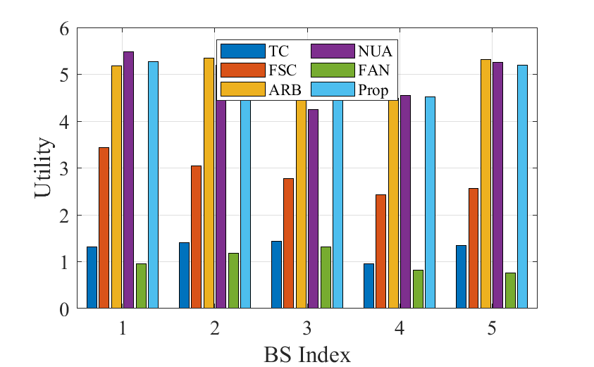
Figure 2: Utility of each BS under the concave utility function.

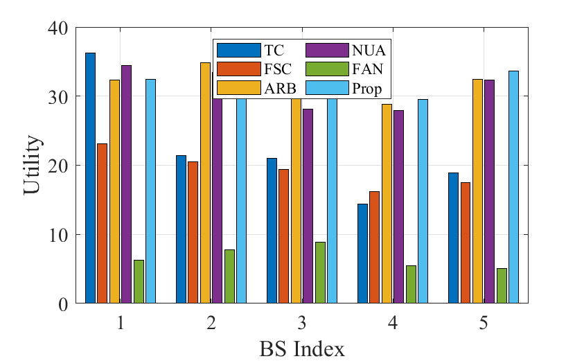
Figure 3: Utility of each BS under the general utility function.

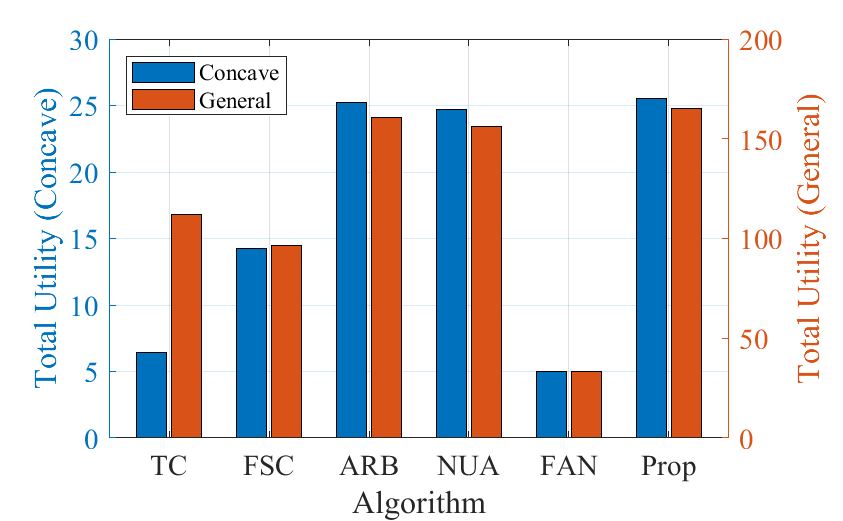
Figure 4: Total utility of different algorithms.

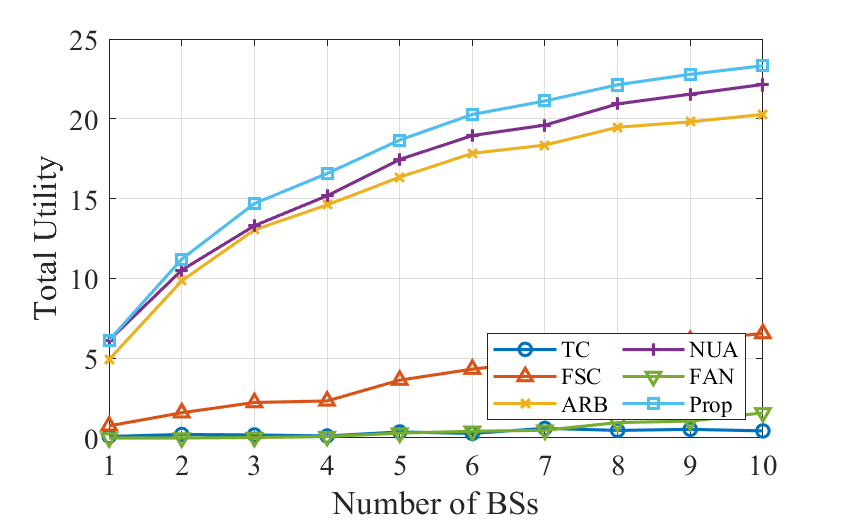
Figure 5: Total utility under different numbers of BSs.

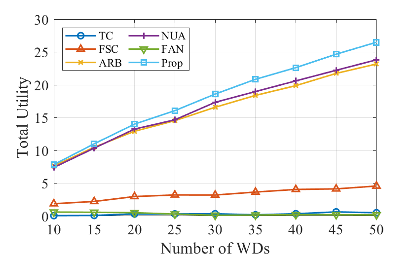
Figure 6: Total utility under different numbers of WDs.

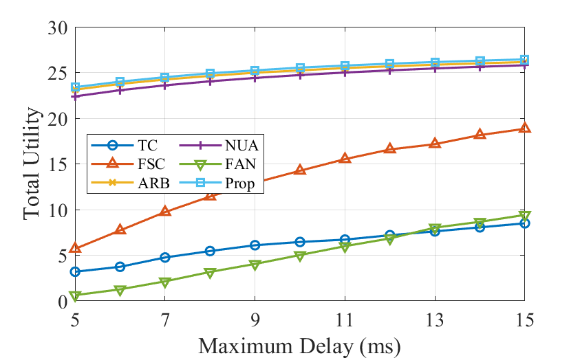
Figure 7: Total utility under different delay requirements.

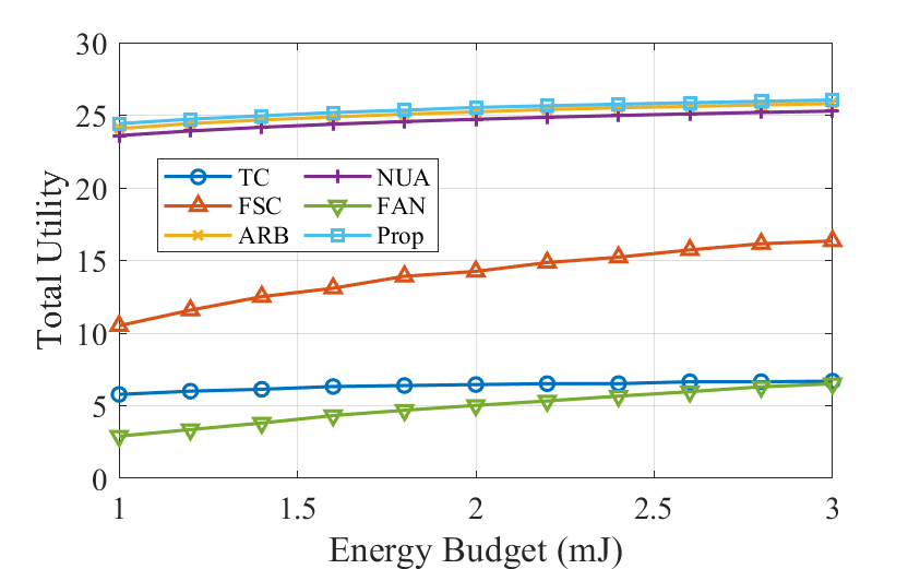
Figure 8: Total utility under different energy budgets.

In this section, extensive simulations are conducted to evaluate the performance of our algorithm. We consider a wireless network consisting of $M=5$ BSs and $N=30$ WDs that are randomly located in a $500$m$\times 500$m square area. For the channel model, we assume the pathloss is $128.1+37.6\log_{10}Dist$ dB and the shadowing factor is $6$ dB, where $Dist$ is the distance (in km) between WDs and BSs.

Our utility function is based on the empirical results about the relationship between result accuracy and computational or communication workload. To model the impact of computational workload $c$ on result accuracy, we conduct curve-fitting on the results given in [23], which shows the accuracy of various models under different computational overhead. We find that the accuracy $A_{c}$ can be well approximated by the following logarithmic function $A_{c}=\eta^{a}_{1}log(\frac{c}{C^{a}})+\eta^{a}_{2}$, where $\eta^{a}_{1},\eta^{a}_{2}$ are parameters corresponding to application $a$ and $C^{a}$ is the computational workload of the maximum DNN model. In our simulation, we set $\eta^{a}_{1}\in\mathcal{U}[0.05,0.08],\eta^{a}_{2}\in\mathcal{U}[0.9,0.95]$, and $C^{a}\in\mathcal{U}[5M,10M]$ cycles, where $\mathcal{U}[a,b]$ represents the uniform distribution on interval $[a,b]$.

According to [19], the relationship between result accuracy $A_{d}$ and communication workload $d$ can be modeled by the following function: $A_{d}=\beta^{a}_{1}(1-\frac{d}{D^{a}})^{\beta^{a}_{2}}+\beta^{a}_{3}$, where $\beta^{a}_{1},\beta^{a}_{2},\beta^{a}_{3}$ are parameters and $D^{a}$ is the maximum data size of the DNN outputs. In our simulation, we set $\beta^{a}_{1}\in\mathcal{U}[-0.75,-0.6],\beta^{a}_{2}\in\mathcal{U}[10,20],\beta^{a}_{3}\in\mathcal{U}[0.9,0.95]$ and $D^{a}\in\mathcal{U}[0.15M,0.25M]$ bits. Intuitively, $\beta^{a}_{3}$ is the result accuracy if all DNN outputs are transmitted to the receiver. Hence, the accuracy discount due to limited data transmission is $A_{d}/\beta^{a}_{3}$. Therefore, we assume the final result accuracy at the receiver side is $A=A_{c}\times A_{d}/\beta^{a}_{3}$. To evaluate our algorithm comprehensively, we consider a concave utility function $u^{a}(c,d)=A$ and a general non-concave function $u^{a}(c,d)=\frac{1}{1-A}$. The values of rest parameters are listed in Table I.

To demonstrate the effectiveness of the proposed algorithm (labeled as “Prop”), we compare it with the following benchmarks. Notice that our algorithm consists of three stages. Unless otherwise specified, each benchmark only differs from our algorithm in one stage.

• Traditional Communication (TC): the raw data is transmitted to the BS without processing.

• Fixed Semantic Communication (FSC): each WD adopts a fixed semantic communication scheme.

• Average RB Allocation (ARB): the RBs are allocated to each associated WD evenly.

• Nearest User Association (NUA): the WDs are associated with the nearest BSs.

• FSC+ARB+NUA (FAN): we use the above three algorithms to produce decisions in each stage respectively.

For TC, we assume the size of raw data satisfies $D_{raw}\in\mathcal{U}[0.4M,0.8M]$ bits. If WD $n$ successfully transmits the raw data under the delay and energy constraints, then the BS can use the maximum DNN model to process the raw data, which leads to result accuracy $\eta^{a}_{2}$. For FSC, the utilized fixed semantic communication scheme is $c=D^{a}/2$ and $d=D^{a}/2$. The data presented in this section are the average of ten repeated experiments with different random seeds.

In Fig. 4 and Fig. 4, we show the utility of each BS under the concave and general utility functions, respectively. In both cases, our algorithm achieves the largest utility at all BSs, except for BS $5$, where NUA outperforms our algorithm. This is because there are more WDs around BS $5$ and they are all associated with BS $5$ in NUA, hence leading to a high utility. In our algorithm, however, we will associate part of these WDs with other BSs to achieve better load balance. As a result, the total utility of all BSs (which is shown in Fig. 4) produced by our algorithm is higher than that of NUA. Another algorithm that has comparable performance is ARB. This is not surprising because the marginal gain of result accuracy drops very quickly with the increase of $d$. Consequently, the marginal gain of utility also drops rapidly with the growth of allocated RBs. This guarantees the average allocation of RBs can achieve close-to-optimal results.

Compared to the previous algorithms, the performance of TC and FSC degrades significantly. The problem in TC and FSC is similar: they both adopt fixed transmission schemes so they are unable to efficiently utilize resources when dealing with heterogeneous users and networks. An interesting observation is that the performance of FAN is even significantly worse than TC. This indicates that adopting semantic communication alone does not necessarily enhance system performance if the resource allocation is not optimized. According to Fig. 4, most algorithms exhibit similar performance under the two different utility functions, except for TC. This is because, under the general utility function, the utility is the reciprocal of one minus accuracy, hence the utility increases very quickly when the accuracy approaches one. This is beneficial for TC as it achieves particularly high accuracy when a WD successfully transmits the raw data to the BS.

To understand the impact of network scale on algorithm performance, Fig. 7 and Fig. 7 demonstrate the total utility of all algorithms under different numbers of BSs and WDs. Due to space limitations, we only present the data under the concave utility function, but the result is similar under the general utility function. From Fig. 7, one can observe that the utility of all algorithms increases with the number of BSs. However, when the number of BSs exceeds 6, the utility gains for Prop, ARB, and NUA are very limited. In contrast, the algorithms that adopt fixed transmission schemes maintain a relatively high growth rate. However, in Fig. 7, the growth trend is exactly the opposite. Specifically, the total utility of Prop, ARB, and NUA grows continuously, indicating their ability to serve more WDs with existing communication resources. The only algorithm showing a decreased utility is FAN. This is because FAN adopts the average allocation of RBs, so the number of RBs allocated to each WD becomes less when there are more WDs. Since FAN also employs a fixed transmission scheme, some WDs are unable to complete the transmission under increasingly less RBs, hence resulting in zero utility.

In addition to network scale, we also investigated the impact of delay and energy constraints on the algorithm results, as shown in Fig. 7 and Fig. 8. The algorithms most sensitive to delay are FSC and FAN, because an increase in delay allows WDs to process data in a more energy-efficient manner, thereby improving the probability of successful transmission. The impact of energy budgets on utility is similar, but overall, its effect is less pronounced compared to delay.

VI Conclusion

In this paper, we have studied the joint optimization of user association and resource allocation in multi-cell semantic communication networks. We introduced the concept of adaptive semantic communication and proposed a three-stage algorithm to maximize the total utility. Numerical results indicate that the performance of semantic communication can significantly outperform the traditional communication paradigm if we choose appropriate control decisions. In our future work, we will embark on building a real adaptive semantic communication system and refine our algorithm based on the experimental results in practical scenarios.

Appendix A Proof of Theorem 1

According to condition (i), when WD $n$ is specified, the corresponding application $a$ is also determined. For convenience, we use $u_{n}$ to denote $u^{a}_{0}$. Since its utility function is binary, its utility can only be $0$ or $u_{n}$. When its utility is $0$, we do not need to associate it with any BS. Therefore, without loss of generality, we can assume $c_{n}=c^{a}_{0}$, $d_{n}=d^{a}_{0}$, and WD $n$ takes utility $u_{n}$ if it is associated with some BS $m$. Then the objective function of problem (8) can be written as $\sum_{n\in\mathcal{N}}\sum_{m\in\mathcal{M}}x^{m}_{n}u_{n}$.

According to condition (ii), the energy constraint (8c) is redundant and we can set $f_{n}=f^{max}_{n}$ and $P_{n}=P^{max}_{n}$. Since both $f_{n}$ and $c_{n}$ are fixed, the computation time $T^{c}_{n}$ becomes a constant. Therefore, the delay constraint (8b) is equivalent to $T^{t}_{n}\leq T^{max}-T^{c}_{n}$, where the right-hand side is a constant. By using condition (iii), the delay constraint (8b) can be further transformed to $z^{m}_{n}\geq x^{m}_{n}C_{n}$, where $C_{n}$ is a constant independent of $m$. Combining with constraint (5) and (8g) we can obtain an equivalent constraint on $x^{m}_{n}$:

$$\sum_{n\in\mathcal{N}}x^{m}_{n}\lceil C_{n}\rceil\leq K_{m},\quad\forall m\in\mathcal{M},$$

where $\lceil\cdot\rceil$ is the ceiling function that returns the smallest integer which is greater than or equal to the input value. As a result, the original problem (8) becomes a standard $0$-$1$ multiple knapsack problem, which is known to be strongly NP-hard [32].

Appendix B Proof of Theorem 2

We prove by contradiction. We first show that (12) must be satisfied. If $E^{c}_{n}+E^{t}_{n}<E^{max}_{n}$, then we can assign the extra energy to the data transmission process, i.e. let $P_{n}^{\prime}=P_{n}^{*}+(E^{max}_{n}-E^{c}_{n}-E^{t}_{n})/T^{t}_{n}$. Apparently, $(f^{*}_{n},P_{n}^{\prime})$ is also a feasible solution of problem (10) but produces larger $d_{n}$ than $(f^{*}_{n},P^{*}_{n})$, contradicting the fact that $(f^{*}_{n},P^{*}_{n})$ is optimal.

Next, we show that (11) must be satisfied. If $T^{c}_{n}+T^{t}_{n}<T^{max}$, then we can assign the extra time to the computation process, i.e. let the new computation time be $T^{c,\prime}_{n}=T^{max}-T^{t}_{n}$. To process $c_{n}$ workload in $T^{c,\prime}_{n}$, the corresponding CPU frequency is $f_{n}^{\prime}=f_{n}^{*}-\frac{(T^{max}-T^{t}_{n}-T^{c}_{n})c_{n}}{T^{c}_{n}(T^{max}-T^{t}_{n})}$. Since $f_{n}^{\prime}<f_{n}^{*}$, we can save an amount of $\Delta E^{c}_{n}=c_{n}\gamma_{n}[(f_{n}^{*})^{2}-(f_{n}^{\prime})^{2}]$ energy for the computation process. Then the saved energy can be assigned to the communication process to achieve a larger $d_{n}$, i.e. $P_{n}^{\prime}=P^{*}_{n}+\Delta E^{c}_{n}/T^{t}_{n}$. One can easily verify that $(f_{n}^{\prime},P_{n}^{\prime})$ is feasible and produces larger $d_{n}$ than $(f_{n}^{*},P_{n}^{*})$, which results in a contradiction.

Appendix C Proof of Theorem 3

We only need to prove the second derivative is non-positive. For brevity, we temporarily drop the subscript $n$ and superscript $m$ in $\hat{z}^{m}_{n}$. Let $(c^{*}(\hat{z}),d^{*}(\hat{z}))$ be the optimal computation and communication workload pair when the allocated number of RBs is $\hat{z}$. Since $u^{a}(c,d)$ is non-descreasing, we can safely assume $d^{*}(\hat{z})=d^{max}(c^{*}(\hat{z}),\hat{z})$. Then we have

$$\frac{\mathop{}\!\mathrm{d}{u}^{*}_{n}(\hat{z})}{\mathop{}\!\mathrm{d}\hat{z}} =\frac{\mathop{}\!\mathrm{d}u^{a}\left(c^{*}(\hat{z}),d^{*}(\hat{z})\right)}{\mathop{}\!\mathrm{d}\hat{z}}$$

$$=\frac{\partial u^{a}}{\partial c^{*}}\times\frac{\mathop{}\!\mathrm{d}c^{*}}{\mathop{}\!\mathrm{d}\hat{z}}+\frac{\partial u^{a}}{\partial d^{*}}\times\frac{\mathop{}\!\mathrm{d}d^{*}}{\mathop{}\!\mathrm{d}\hat{z}}$$

$$=\frac{\partial u^{a}}{\partial c^{*}}\times\frac{\mathop{}\!\mathrm{d}c^{*}}{\mathop{}\!\mathrm{d}\hat{z}}+\frac{\partial u^{a}}{\partial d^{*}}\times\left(\frac{\partial d^{*}}{\partial c^{*}}\times\frac{\mathop{}\!\mathrm{d}c^{*}}{\mathop{}\!\mathrm{d}\hat{z}}+\frac{\partial d^{*}}{\partial\hat{z}}\right)$$

$$=\frac{\mathop{}\!\mathrm{d}c^{*}}{\mathop{}\!\mathrm{d}\hat{z}}\left(\frac{\partial u^{a}}{\partial c^{*}}+\frac{\partial u^{a}}{\partial d^{*}}\times\frac{\partial d^{*}}{\partial{c^{*}}}\right)+\frac{\partial u^{a}}{\partial d^{*}}\times\frac{\partial d^{*}}{\partial\hat{z}}.$$ (20)

According to the discussion in Section IV-A, after plugging $f^{*}_{n}(c_{n})$ into $d_{n}$, $d^{max}_{n}$ equals $z^{m}_{n}$ multiplies a function of $c_{n}$, denoted by $g(c_{n})$. Therefore, we can express $d^{*}(\hat{z})$ as

$$d^{*}(\hat{z})=\hat{z}g(c^{*}(\hat{z})).$$ (21)

Since $c^{*}(\hat{z})$ is optimal, we have

$$\frac{\mathop{}\!\mathrm{d}u^{a}}{\mathop{}\!\mathrm{d}c^{*}}=\frac{\partial u^{a}}{\partial c^{*}}+\frac{\partial u^{a}}{\partial d^{*}}\times\frac{\partial d^{*}}{\partial c^{*}}=0.$$ (22)

Substituting (21) and (22) into (20) yields $\frac{\mathop{}\!\mathrm{d}{u}^{*}_{n}(\hat{z})}{\mathop{}\!\mathrm{d}\hat{z}}=\frac{\partial u^{a}}{\partial d^{*}}\times g(c^{*}(\hat{z}))$. Then the second derivative of ${u}^{*}_{n}(\hat{z})$ is

$$\frac{\mathop{}\!\mathrm{d}^{2}{u}^{*}_{n}(\hat{z})}{\mathop{}\!\mathrm{d}\hat{z}^{2}}=\frac{\partial u^{a}}{\partial d^{*}}\times\frac{\partial g}{\partial c^{*}}\times\frac{\partial c^{*}}{\partial\hat{z}}.$$ (23)

Since $u^{a}(c,d)$ is non-decreasing, the first term in (23) is non-negative. For the second term, it is apparent that $d^{max}(c)$ is non-increasing with respect to $c$, hence $g(c^{*}(\hat{z}))$ is also non-increasing with respect to $c^{*}(\hat{z})$, so the second term is non-positive. Therefore, we only need to prove the third term is non-negative. Let $\alpha>1$ be an arbitrary constant. It is easy to verify that $(c^{*}(\hat{z}),\alpha d^{*}(\hat{z}))$ is achievable when the allocated RB grows to $\alpha\hat{z}$. The partial derivative of $u^{a}(c,d)$ at $(c^{*}(\hat{z}),\alpha d^{*}(\hat{z}))$ satisfies

$$\frac{\mathop{}\!\mathrm{d}u^{a}}{\mathop{}\!\mathrm{d}c^{*}}\Big{|}_{(c^{*}(\hat{z}),\alpha d^{*}(\hat{z}))}$$

$$\quad=\frac{\partial u^{a}}{\partial c^{*}}\Big{|}_{(c^{*},\alpha d^{*})}+\frac{\partial u^{a}}{\partial d^{*}}\Big{|}_{(c^{*},\alpha d^{*})}\times\frac{\partial d^{*}}{\partial c^{*}}\Big{|}_{(c^{*},\alpha\hat{z})}$$

$$\quad\geq\frac{\partial u^{a}}{\partial c^{*}}\Big{|}_{(c^{*},d^{*})}+\frac{1}{\alpha}\frac{\partial u^{a}}{\partial d^{*}}\Big{|}_{(c^{*},d^{*})}\times\alpha\frac{\partial d^{*}}{\partial c^{*}}\Big{|}_{(c^{*},\hat{z})}$$

$$\quad=\frac{\partial u^{a}}{\partial c^{*}}\Big{|}_{(c^{*},d^{*})}+\frac{\partial u^{a}}{\partial d^{*}}\Big{|}_{(c^{*},d^{*})}\times\frac{\partial d^{*}}{\partial c^{*}}\Big{|}_{(c^{*},\hat{z})}=0$$

where the inequality is based on Assumption 2, Assumption 3, $\frac{\partial d^{*}}{\partial c^{*}}\leq 0$, and the fact that $\frac{\partial d^{*}}{\partial c^{*}}$ is linear with respect to $\hat{z}$. Since the partial derivative is non-negative, we will obtain a larger utility if we increase the value of $c^{*}(\hat{z})$. Hence, when the allocated RB is $\alpha\hat{z}$, the optimal computation workload is larger than $c^{*}(\hat{z})$, i.e. $c^{*}(\alpha\hat{z})\geq c^{*}(\hat{z})$. Since the value of $\alpha$ is arbitrary, we can conclude that $c^{*}(\hat{z})$ is non-decreasing with respect to $\hat{z}$, which completes the proof.

References

- [1] C. E. Shannon, “A mathematical theory of communication,” The Bell System Technical Journal, vol. 27, pp. 379–423, 1948. [Online]. Available: http://plan9.bell-labs.com/cm/ms/what/shannonday/shannon1948.pdf
- [2] J. Bao, P. Basu, M. Dean, C. Partridge, A. Swami, W. Leland, and J. A. Hendler, “Towards a theory of semantic communication,” in 2011 IEEE Network Science Workshop. IEEE, 2011, pp. 110–117.
- [3] Z. Qin, X. Tao, J. Lu, W. Tong, and G. Y. Li, “Semantic communications: Principles and challenges,” arXiv preprint arXiv:2201.01389, 2021.
- [4] D. Gündüz, Z. Qin, I. E. Aguerri, H. S. Dhillon, Z. Yang, A. Yener, K. K. Wong, and C.-B. Chae, “Beyond transmitting bits: Context, semantics, and task-oriented communications,” IEEE Journal on Selected Areas in Communications, vol. 41, no. 1, pp. 5–41, 2022.
- [5] Q. Ye, B. Rong, Y. Chen, M. Al-Shalash, C. Caramanis, and J. G. Andrews, “User association for load balancing in heterogeneous cellular networks,” IEEE Transactions on Wireless Communications, vol. 12, no. 6, pp. 2706–2716, 2013.
- [6] D. Bethanabhotla, O. Y. Bursalioglu, H. C. Papadopoulos, and G. Caire, “Optimal user-cell association for massive mimo wireless networks,” IEEE Transactions on Wireless Communications, vol. 15, no. 3, pp. 1835–1850, 2015.
- [7] Q. Ye, O. Y. Bursalioglu, H. C. Papadopoulos, C. Caramanis, and J. G. Andrews, “User association and interference management in massive mimo hetnets,” IEEE Transactions on Communications, vol. 64, no. 5, pp. 2049–2065, 2016.
- [8] J. G. Andrews, S. Singh, Q. Ye, X. Lin, and H. S. Dhillon, “An overview of load balancing in hetnets: Old myths and open problems,” IEEE Wireless Communications, vol. 21, no. 2, pp. 18–25, 2014.
- [9] D. Liu, L. Wang, Y. Chen, M. Elkashlan, K.-K. Wong, R. Schober, and L. Hanzo, “User association in 5g networks: A survey and an outlook,” IEEE Communications Surveys & Tutorials, vol. 18, no. 2, pp. 1018–1044, 2016.
- [10] M. Sheng, C. Yang, Y. Zhang, and J. Li, “Zone-based load balancing in lte self-optimizing networks: A game-theoretic approach,” IEEE transactions on vehicular technology, vol. 63, no. 6, pp. 2916–2925, 2013.
- [11] C. E. Shannon and W. Weaver, The mathematical theory of communication, by CE Shannon (and recent contributions to the mathematical theory of communication), W. Weaver. University of illinois Press, 1949.
- [12] H. Xie, Z. Qin, G. Y. Li, and B.-H. Juang, “Deep learning enabled semantic communication systems,” IEEE Transactions on Signal Processing, vol. 69, pp. 2663–2675, 2021.
- [13] D. Huang, F. Gao, X. Tao, Q. Du, and J. Lu, “Toward semantic communications: Deep learning-based image semantic coding,” IEEE Journal on Selected Areas in Communications, vol. 41, no. 1, pp. 55–71, 2022.
- [14] Z. Weng and Z. Qin, “Semantic communication systems for speech transmission,” IEEE Journal on Selected Areas in Communications, vol. 39, no. 8, pp. 2434–2444, 2021.
- [15] P. Jiang, C.-K. Wen, S. Jin, and G. Y. Li, “Wireless semantic communications for video conferencing,” IEEE Journal on Selected Areas in Communications, vol. 41, no. 1, pp. 230–244, 2022.
- [16] L. Yan, Z. Qin, R. Zhang, Y. Li, and G. Y. Li, “Resource allocation for text semantic communications,” IEEE Wireless Communications Letters, vol. 11, no. 7, pp. 1394–1398, 2022.
- [17] ——, “Qoe-aware resource allocation for semantic communication networks,” in GLOBECOM 2022-2022 IEEE Global Communications Conference. IEEE, 2022, pp. 3272–3277.
- [18] Y. Wang, M. Chen, T. Luo, W. Saad, D. Niyato, H. V. Poor, and S. Cui, “Performance optimization for semantic communications: An attention-based reinforcement learning approach,” IEEE Journal on Selected Areas in Communications, vol. 40, no. 9, pp. 2598–2613, 2022.
- [19] H. Zhang, H. Wang, Y. Li, K. Long, and A. Nallanathan, “Drl-driven dynamic resource allocation for task-oriented semantic communication,” IEEE Transactions on Communications, 2023.
- [20] W. Zhang, Y. Wang, M. Chen, T. Luo, and D. Niyato, “Optimization of image transmission in a cooperative semantic communication networks,” arXiv preprint arXiv:2301.00433, 2023.
- [21] C. Liu, C. Guo, Y. Yang, and N. Jiang, “Adaptable semantic compression and resource allocation for task-oriented communications,” arXiv preprint arXiv:2204.08910, 2022.
- [22] J. Yu, L. Yang, N. Xu, J. Yang, and T. Huang, “Slimmable neural networks,” in International Conference on Learning Representations, 2019.
- [23] J. Yu and T. S. Huang, “Universally slimmable networks and improved training techniques,” in Proceedings of the IEEE/CVF international conference on computer vision, 2019, pp. 1803–1811.
- [24] J. Yu and T. Huang, “Autoslim: Towards one-shot architecture search for channel numbers,” arXiv preprint arXiv:1903.11728, 2019.
- [25] H. Cai, C. Gan, T. Wang, Z. Zhang, and S. Han, “Once-for-all: Train one network and specialize it for efficient deployment,” in International Conference on Learning Representations, 2020.
- [26] M. Weiser, B. Welch, A. Demers, and S. Shenker, “Scheduling for reduced cpu energy,” Mobile Computing, pp. 449–471, 1996.
- [27] A. P. Chandrakasan, S. Sheng, and R. W. Brodersen, “Low-power cmos digital design,” IEICE Transactions on Electronics, vol. 75, no. 4, pp. 371–382, 1992.
- [28] H. Kim, G. De Veciana, X. Yang, and M. Venkatachalam, “Distributed -optimal user association and cell load balancing in wireless networks,” IEEE/ACM Transactions on Networking, vol. 20, no. 1, pp. 177–190, 2011.
- [29] G. Athanasiou, P. C. Weeraddana, C. Fischione, and L. Tassiulas, “Optimizing client association for load balancing and fairness in millimeter-wave wireless networks,” IEEE/ACM Transactions on Networking, vol. 23, no. 3, pp. 836–850, 2014.
- [30] W. Saad, Z. Han, R. Zheng, M. Debbah, and H. V. Poor, “A college admissions game for uplink user association in wireless small cell networks,” in IEEE INFOCOM 2014-IEEE Conference on Computer Communications. IEEE, 2014, pp. 1096–1104.
- [31] T. Han and N. Ansari, “A traffic load balancing framework for software-defined radio access networks powered by hybrid energy sources,” IEEE/ACM Transactions on Networking, vol. 24, no. 2, pp. 1038–1051, 2015.
- [32] S. Martello and P. Toth, Knapsack problems: algorithms and computer implementations. John Wiley & Sons, Inc., 1990.