Bagged Regularized $k$-Distances for Anomaly Detection

Abstract

We consider the paradigm of unsupervised anomaly detection, which involves the identification of anomalies within a dataset in the absence of labeled examples. Though distance-based methods are top-performing for unsupervised anomaly detection, they suffer heavily from the sensitivity to the choice of the number of the nearest neighbors. In this paper, we propose a new distance-based algorithm called bagged regularized $k$-distances for anomaly detection (BRDAD) converting the unsupervised anomaly detection problem into a convex optimization problem. Our BRDAD algorithm selects the weights by minimizing the surrogate risk, i.e., the finite sample bound of the empirical risk of the bagged weighted $k$-distances for density estimation (BWDDE). This approach enables us to successfully address the sensitivity challenge of the hyperparameter choice in distance-based algorithms. Moreover, when dealing with large-scale datasets, the efficiency issues can be addressed by the incorporated bagging technique in our BRDAD algorithm. On the theoretical side, we establish fast convergence rates of the AUC regret of our algorithm and demonstrate that the bagging technique significantly reduces the computational complexity. On the practical side, we conduct numerical experiments on anomaly detection benchmarks to illustrate the insensitivity of parameter selection of our algorithm compared with other state-of-the-art distance-based methods. Moreover, promising improvements are brought by applying the bagging technique in our algorithm on real-world datasets.

1 Introduction

Anomaly detection refers to the process of identifying patterns or instances that deviate significantly from the expected behavior within a dataset [12]. It has been widely and carefully studied within diverse research areas and application domains, including industrial engineering [20, 51], medicine [21, 47], cyber security [22, 40], earth science [35, 13], and finance [34, 29], etc. For further discussions on anomaly detection techniques and applications, we refer readers to the survey of [38].

Based on the availability of labeled data, anomaly detection problems can be classified into three main paradigms. The first is the supervised paradigm where both the normal and anomalous instances are labeled. As mentioned in [3] and [50], researchers often employ existing binary classifiers in this case. The second is the semi-supervised paradigm where the training data only consists of normal samples, and the goal is to identify anomalies that deviate from the normal samples. [6, 55]. Perhaps the most flexible yet challenging paradigm is the unsupervised paradigm [3, 25], where no labeled examples are available to train an anomaly detector. For the remainder of this paper, we only focus on the unsupervised paradigm, where we do not assume any prior knowledge of labeled data.

The existing algorithms in the literature on unsupervised anomaly detection can be roughly categorized into three main categories: The first category is distance-based methods, which determine an anomaly score based on the distance between data points and their neighboring points. For example, $k$-nearest neighbors ($k$-NN) [39] calculate the anomaly score of an instance based on the distance to its $k$-th nearest neighbor, distance-to-measure (DTM) [25] introduces a novel distance metric based on the distances of the first $k$-nearest neighbors, and local outlier factor (LOF) [11] computes the anomaly score by quantifying the deviation of the instance from the local density of its neighboring data points. The second category is forest-based methods, which compute anomaly scores based on tree structures. For instance, isolation forest (iForest) [33] constructs an ensemble of trees to isolate data points and quantifies the anomaly score of each instance based on its distance from the leaf node to the root in the constructed tree and partial identification forest (PIDForest) [24] computes the anomaly score of a data point by identifying the minimum density of data points across all subcubes partitioned by decision trees. The third category is kernel-based methods such as the one-class SVM (OCSVM) [42], which defines a hyperplane to maximize the margin between the origin and normal samples. It has been empirically shown [4, 5, 25] that distance-based and forest-based methods are the top-performing methods across a broad range of real-world datasets. Moreover, experiments in [25] suggest that distance-based methods show their advantage on high-dimensional datasets, as forest-based methods are likely to neglect a substantial number of features when dealing with high-dimensional data. Unfortunately, it is widely acknowledged that distance-based methods suffer from the sensitivity to the choice of the hyper-parameter $k$ [2]. This problem is particularly severe in unsupervised learning tasks because the absence of labeled data makes it difficult to guide the selection of hyper-parameters. To the best of our knowledge, no algorithm in the literature effectively solves the aforementioned sensitivity problem. Besides, while distance-based methods are crucial and efficient for identifying anomalies, they pose a challenge in scenarios with a high volume of data samples, owing to the need for a considerable expansion in the search for nearest neighbors, leading to a notable increase in computational overhead. Therefore, there also remains a great challenge for distance-based algorithms to improve their computational efficiency.

Under this background, in this paper, we propose a distance-based algorithm named bagged regularized $k$-distances for anomaly detection (BRDAD), which converts the weight selection problem in unsupervised anomaly detection into a minimization problem. More precisely, we first establish the surrogate risk, i.e., the finite sample bound of the empirical risk of the bagged weighted $k$-distances for density estimation (BWDDE) associated with the weighted $k$-distances. At each bagging round, we then select the weights by minimizing the surrogate risk on each subsampling data and call the corresponding weighted $k$-distance as regularized $k$-distance. By taking the average of these regularized $k$-distances, namely bagged regularized $k$-distances, as the anomaly scores for each instance, our BRDAD sorts the data using the bagged regularized $k$-distances in descending order and identifies the first $m$ instances as the top $m$ anomalies. It is worth mentioning that BRDAD has two advantages. Firstly, the surrogate risk minimization (SRM) approach enables us to successfully address the sensitivity of parameter choices in distance-based algorithms. Secondly, when dealing with large-scale datasets, the incorporated bagging technique helps to address the computational efficiency issue in our proposed distance-based method.

The contributions of this paper are summarized as follows.

(i) We propose a new distance-based algorithm BRDAD that prevents the sensitivity of the hyper-parameter selection in unsupervised anomaly detection problems by formulating it as a convex optimization problem. Moreover, the incorporated bagging technique in BRDAD improves the computational efficiency of our distance-based algorithm.

(ii) From the theoretical perspective, we establish fast convergence rates of the AUC regret of BRDAD. Moreover, we show that with relatively few bagging rounds $B$, the number of iterations in the optimization problem at each bagging round can be reduced substantially. This demonstrates that the bagging technique significantly reduces computational complexity.

(iii) From the experimental perspective, we conduct numerical experiments to illustrate the effectiveness of our proposed BRDAD. Firstly, we empirically verify the convergence of the solution to the SRM problem and the convergence of the mean absolute error (MAE) of BRDDE. Then, we demonstrate the effectiveness of our proposed BRDAD compared with other distance-based, forest-based, and kernel-based methods on anomaly detection benchmarks. Furthermore, we conduct parameter analysis on the bagging rounds $B$ on the proposed BRDAD, empirically demonstrating that appropriate values of $B$ such as 5 or 10 yield better performance. Finally, we provide an illustrative example to show the sensitivity of parameter selection of $k$ for distance-based algorithms including $k$-NN, DTM, and LOF. By contrast, BRDAD avoids the aforementioned sensitivity issue.

The remainder of this paper is organized as follows. In Section 2, we introduce some preliminaries related to anomaly detection and propose our BRDAD algorithm. We provide basic assumptions and theoretical results on the convergence rates of BRDDE and BRDAD in Section 3. Some comments and discussions concerning the theoretical results will also be provided in this section. We present the error and complexity analysis of our algorithm in Section 4. Some comments concerning the time complexity will also be provided in this section. We verify the theoretical findings of our algorithm by conducting numerical experiments in Section 5. We also conduct numerical experiments to compare our algorithm with other state-of-the-art algorithms for anomaly detection on real-world datasets in this Section. All the proofs of Sections 2, 3, and 4 can be found in Section 6. We conclude this paper in Section 7.

2 Methodology

We present our methodology in this section. We first introduce basic notations and concepts in Section 2.1. Then, in Section 2.2, we propose the bagged weighted $k$-distances for density estimation (BWDDE) to show that the bagged weighted $k$-distances can be used for anomaly detection. Then, in Section 2.3, we convert the weight selection problem for density estimation into the SRM problem, i.e., minimizing the finite sample bound of empirical risk of the BWDDE. Finally, the weights obtained by solving the SRM problem are utilized to construct our main algorithm, named bagged regularized $k$-distances for anomaly detection (BRDAD).

2.1 Preliminaries

We begin by introducing some fundamental notations that will frequently appear. Suppose that independent data $D_{n}:=\{X_{1},\ldots,X_{n}\}$ are drawn from an unknown distribution $\mathrm{P}$ that is absolutely continuous with respect to the Lebesgue measure $\mu$ and admits a unique invariant Lebesgue density $f$. We denote the support of $f$ as $\mathcal{X}$, i.e. $\mathcal{X}=\{x:f(x)>0\}$. Recall that for $1\leq p<\infty$, the $\ell_{p}$-norm is defined as $\|x\|_{p}:=(x_{1}^{p}+\cdots+x_{d}^{p})^{1/p}$, and the $\ell_{\infty}$-norm is defined as $\|x\|_{\infty}:=\max_{i=1,\ldots,d}|x_{i}|$. For a measurable function $g:\mathcal{X}\to\mathbb{R}$, we define the $L_{p}$-norm as $\|g\|_{p}:=\big{(}\int_{\mathcal{X}}|g(x)|^{p}\,dx\big{)}^{1/p}$. A ball in Euclidean space $\mathbb{R}^{d}$ centered at $x\in\mathbb{R}^{d}$ with radius $r\in(0,+\infty)$ is denoted by $B(x,r)$. In addition, for $n\in\mathbb{N}_{+}$, we write $[n]:=\{1,\ldots,n\}$ as the set containing integers from $1$ to $n$ and $\mathcal{W}_{n}:=\{(w_{1},\ldots,w_{n})\in\mathbb{R}^{n}:\sum_{i=1}^{n}w_{i}=1,\ w_{i}\geq 0,\ i\in[n]\}$. For any $x\in\mathbb{R}$, let $\lfloor x\rfloor$ be the largest integer less than or equal to $x$ and $\lceil x\rceil$ be the smallest ingeter larger than or equal to $x$.

Throughout this paper, we use $a\vee b=\max\{a,b\}$ and $a\wedge b=\min\{a,b\}$. Moreover, we use the following notations to compare the magnitudes of quantities: $a_{n}\lesssim b_{n}$ or $a_{n}=\mathcal{O}(b_{n})$ indicates that there exists a positive constant $c>0$ that is independent of $n$ such that $a_{n}\leq cb_{n}$; $a_{n}\gtrsim b_{n}$ implies that there exists a positive constant $c>0$ such that $a_{n}\geq cb_{n}$; and $a_{n}\asymp b_{n}$ means that $a_{n}\lesssim b_{n}$ and $b_{n}\lesssim a_{n}$ hold simultaneously. Finally, we interchangeably use $C$, $c$, and $c^{\prime}$ to represent positive constants, whose values may differ among various lemmas, propositions, theorems, and corollaries.

2.2 Bagged Weighted $k$-Distances for Anomaly Detection

The learning goal of anomaly detection is to identify observations that deviate significantly from the majority of the data. Anomalies are typically rare and different from the expected behavior of the data set. Among the various methods employed for unsupervised anomaly detection, distance-based methods stand out as a widely adopted approach to address this challenge, which relies on the concept of measuring distances between data points and their nearest neighbors to identify anomalies. Before we proceed, we introduce some basic notations. For any $x\in\mathbb{R}^{d}$ and a dataset $D_{n}$, we denote $X_{(k)}(x;D_{n})$ as the $k$-th nearest neighbor of $x$ in $D_{n}$. Then, we denote $R_{n,(k)}(x):=\bigl{\|}x-X_{(k)}(x;D_{n})\bigr{\|}_{2}$ as the distance between $x$ and $X_{(k)}(x;D_{n})$, termed as the $k$-nearest neighbor distance, or $k$-distance of $x$ in $D_{n}$.

Although distance-based methods are important and effective approaches for anomaly detection. When dealing with a large number of data points, a significant increase in the number of nearest neighbors to be searched occurs in distance-based methods, which introduces substantial computational overhead. To deal with the efficiency issues on the $k$-distance, we introduce the bagging technique by averaging the weighted $k$-distances on the disjoint sub-datasets randomly drawn from the original data $D_{n}$ without replacement. Specifically, let $B$ be the number of bagging rounds pre-specified by the user. We randomly and evenly divide the data $D_{n}$ into $B$ disjoint sub-datasets of size $s$, namely $\{D_{s}^{b}\}_{b=1}^{B}$. For the sake of convenience, we assume that $n$ is divisible by $B$ and $n=Bs$. Additionally, the probability distribution of this sub-sampling procedure is denoted as $\mathrm{P}_{B}$. In each subset $D^{b}_{s}$, $b\in[B]$, let $R_{s,(k)}^{b}(x):=\bigl{\|}x-X_{(k)}(x;D_{s}^{b})\bigr{\|}_{2}$ be the $k$-distance of $x$ in $D_{s}^{b}$ and the weighted $k$-distance be defined as $R^{w,b}_{s}(x):=\sum_{i=1}^{s}w_{i}^{b}R_{s,(i)}^{b}(x),\ w\in\mathcal{W}_{s}$. The average of these weighted $k$-distances across the $B$ sub-datasets is defined as the bagged weighted $k$-distances, i.e.

$$R_{n}^{B}(x):=\frac{1}{B}\sum_{b=1}^{B}R^{w,b}_{s}(x).$$

With these preparations, we apply the bagged weighted $k$-distances in the context of the density-based anomaly detection paradigm, which seeks to identify anomalies based on their densities in the feature space. To this end, we define the bagged weighted $k$-distances for density estimation (BWDDE) by

$$f^{B}_{n}(x):=\frac{1}{V_{d}{R}_{n}^{B}(x)^{d}}\biggl{(}\frac{1}{B}\sum_{b=1}^{B}\sum_{i=1}^{s}w_{i}^{b}(i/s)^{1/d}\biggr{)}^{d},$$ (1)

where $V_{d}:=\pi^{d/2}/\Gamma(d/2+1)$ is the volume of the unit ball. By estimating the density of data points in a dataset, we can find potential anomalies in regions of low density. More precisely, according to their BWDDEs, the dataset $D_{n}=\{X_{1},\ldots,X_{n}\}$ can be sorted in a sequence of ascending order, denote as $\{\widetilde{X}_{1},\ldots,\widetilde{X}_{n}\}$, i.e., we have $f_{n}^{B}(\widetilde{X}_{1})\leq\cdots\leq f_{n}^{B}(\widetilde{X}_{n})$. If the number of anomalies is specified as $m$, then the $m$ data points with the smallest BWDDEs in the dataset are identified as anomalies. This approach is grounded in the fundamental principle that anomalies often exhibit significantly lower density compared to normal instances.

2.3 Bagged Regularized $k$-Distances for Anomaly Detection

However, in general, a significant challenge of bagged weighted $k$-distance lies in selecting the appropriate weights assigned to the nearest neighbors for the density estimation (1). These weights have a substantial impact on the accuracy of density estimation and correspondingly the precision of anomaly detection, making their selections a complex task. The simplest way is to take $B=1$, $w_{i}=1$, $i=k$, and $w_{i}=0$, $i\in[n]\setminus\{k\}$. In this case, BWDDE reverts to the standard $k$-NN density estimation [37, 18, 16]. Note that the standard $k$-NN density estimation only uses the information of $k$-th nearest neighbor and ignores the information of other nearest neighbors. A more general approach was proposed by [9] which investigated the general weighted $k$-nearest neighbor density estimation by associating the weights with a given probability measure on $[0,1]$. The probability measure was selected by using a standard leave-one-out cross-validation method [48, 9] based on the $L_{2}$ criterion. However, this parameter selection method is not feasible for high-dimensional datasets since it requires the computation of an integral of the square of the density estimation on the whole space $\mathbb{R}^{d}$. Unfortunately, this integral does not have an explicit expression and thus has to be estimated by the Monte Carlo method. When dealing with high-dimensional datasets, a large number of samples are required to ensure the accuracy. Therefore, it is difficult to determine the weights for nearest neighbors accurately in practical applications, especially for high-dimensional datasets.

In this section, to address such weight selection challenge, we introduce the surrogate risk minimization (SRM) approach, providing an effective means of determining the weights for BWDDE. Specifically, we first establish the surrogate risk, namely, the finite sample bound of the empirical risk of BWDDE w.r.t. to the absolute loss under certain regular assumptions. By minimizing the surrogate risk, which converts the unsupervised weight selection problem for density estimation into a convex optimization problem, we are able to select the weights and obtain the density estimation algorithm called bagged regularized $k$-distances for density estimation (BRDDE). This also enables us to propose our anomaly detection algorithm called bagged regularized $k$-distances for anomaly detection (BRDAD), which shares the same weights with BRDDE.

In the context of density estimation, we consider the absolute loss function $L:\mathcal{X}\times\mathbb{R}\to[0,\infty)$ defined by $L(x,t):=|f(x)-t|$, which measures the discrepancy between the density estimation and the underlying density function $f$, based on a set of observed data points. Specifically, the empirical risk of the BWDDE $f_{n}^{B}$ is given by

$$\mathcal{R}_{L,\mathrm{D}_{n}}(f_{n}^{B}):=\frac{1}{n}\sum_{i=1}^{n}\bigl{|}f_{n}^{B}(X_{i})-f(X_{i})\bigr{|}.$$ (2)

The empirical risk of the BWDDE w.r.t the absolute loss is also called mean absolute error (MAE). As is stated in [17, 28], the absolute loss $L$ is a reasonable choice for density estimation. This is due to its invariance under monotone transformations. Moreover, it is proportional to the total variation metric, facilitating better visualization of the proximity to the actual density function.

Notice that since the underlying density function $f$ in (2) is unknown, the commonly used optimization techniques for parameter selection can not be directly used for the weight selection in density estimation. To deal with this issue, we aim to find a surrogate of the empirical risk $\mathcal{R}_{L,\mathrm{D}_{n}}(f_{n}^{B})$ in (2) and then minimize it to select the weights of the nearest neighbors. To this end, we need to introduce the following regularity assumptions on the underlying probability distribution $\mathrm{P}$.

Assumption 1.

Assume that $\mathrm{P}$ has a Lebesgue density $f$ with bounded support $\mathcal{X}=[0,1]^{d}$.

1. [Lipschitz Continuity] The density $f$ is Lipschitz continuous on $[0,1]^{d}$, i.e., for all $x,y\in[0,1]^{d}$, there exists a constant $c_{L}>0$ such that $|f(x)-f(y)|\leq c_{L}\|x-y\|_{2}$.

2. [Boundness] There exist constants $\overline{c}\geq\underline{c}>0$ such that $\underline{c}\leq f(x)\leq\overline{c}$ for all $x\in\mathcal{X}$.

The smoothness assumption is needed when bounding the variation of the density function, which is commonly adopted in density estimation [16, 30], since it helps to avoid over-fitting the data and provides a more stable estimation of the density. The boundedness assumption is usually adopted to derive the finite sample bounds for density estimations, see, e.g., [30, 54]. Under the above assumption and additional conditions on the weights, the next proposition presents a surrogate of the empirical risk (2).

Proposition 1 (Surrogate Risk).

Let Assumption 1 hold, $L$ be the absolute value loss, the dataset $D_{n}$ be randomly and evenly divided into $B$ disjoint subsets $\{D_{s}^{b}\}_{b=1}^{B}$ with $D_{s}^{b}:=\{X_{1}^{b},\ldots,X_{s}^{b}\}$, and $\overline{R}_{s,(i)}^{b}:=\sum_{j=1}^{s}R_{s,(i)}^{b}(X_{j}^{b})/s$ be the average $i$-distance of $x$ on the subset $D_{s}^{b}$. Furthermore, let $f$ be the underlying density function and $f_{n}^{B}$ be the BWDDE as in (1). Moreover, let $k^{b}:=k(w^{b}):=\sup\{i\in[s]:w^{b}_{i}\neq 0\}$, $\underline{k}:=\min_{b\in[B]}k^{b}$, and $\overline{k}:=\max_{b\in[B]}k^{b}$. Finally, suppose that the following four conditions hold:

1. $s\gtrsim n^{d/(2+d)}(\log n)^{2/(2+d)}$ and $\displaystyle\sum_{i=1}^{c_{n}}w_{i}^{b}\lesssim\log s/k^{b}$ with $c_{n}\asymp\log n$ for $b\in[B]$;

2. $k^{b}\gtrsim\log s$, $\|w^{b}\|_{2}\gtrsim\bigl{(}k^{b}\bigr{)}^{-1/2}$, and $\displaystyle\sum_{i=1}^{s}i^{1/d}w_{i}^{b}\asymp\bigl{(}k^{b}\bigr{)}^{1/d}$ for $b\in[B]$;

3. $\underline{k}\asymp\overline{k}$ and $B\gtrsim\overline{k}\log n$;

4. $\displaystyle\max_{b\in[B]}w^{b}_{i}\leq V_{i}$ for $c_{n}<i\leq s$ and $\displaystyle\sum_{i=c_{n}}^{s}i^{1/d-1/2}V_{i}\lesssim\overline{k}^{1/d-1/2}$.

Then there exists an $N_{1}^{*}\in\mathbb{N}$, which is specified in the proof, such that for all $n\geq N_{1}^{*}$ and $X_{i}^{b}$ satisfying $B(X_{i}^{b},R_{s,(k^{b})}^{b}(X_{i}^{b}))\subset[0,1]^{d}$, $b\in[B]$, there holds

$$L(X_{i}^{b},f_{n}^{B})\lesssim\sqrt{\log s/B}\cdot\|w^{b}\|_{2}+R^{w,b}_{s}(X_{i}^{b})+(\log s)^{2}/B,\qquad i\in[s],\,b\in[B],$$ (3)

with probability $\mathrm{P}^{n}\otimes\mathrm{P}_{B}$ at least $1-1/n^{2}$. As a consequence, we obtain

$$\mathcal{R}_{L,\mathrm{D}_{n}}(f_{n}^{B})\lesssim\mathcal{R}_{L,\mathrm{D_{n}}}^{\mathrm{sur}}(f_{n}^{B}) :=\frac{1}{B}\sum_{b=1}^{B}\biggl{(}\sqrt{\log s/B}\cdot\|w^{b}\|_{2}+\frac{1}{s}\sum_{i=1}^{s}R^{w,b}_{s}(X_{i}^{b})+(\log s)^{2}/B\biggr{)}$$

$$=\frac{1}{B}\sum_{b=1}^{B}\biggl{(}\sqrt{\log s/B}\cdot\|w^{b}\|_{2}+\sum_{i=1}^{s}w_{i}^{b}\overline{R}_{s,(i)}^{b}+(\log s)^{2}/B\biggr{)}.$$ (4)

The expression $\mathcal{R}_{L,\mathrm{D_{n}}}^{\mathrm{sur}}(f_{n}^{B})$ on the right-hand side of (1) is termed as the surrogate risk. Clearly, the smaller the value of the surrogate risk, the higher the accuracy of BWDDE. Condition (i) requires the subsample size $s$ not too small and the weights not concentrated in the first $c_{n}$ nearest neighbors. The first condition in (ii) requires the number of nearest neighbors $k^{b}$ to be at least of the order $\log s$, which coincides with the choice of $k$ with respect to the finite sample bounds established in [16]. On the other hand, the second condition in (ii) requires that the weights should not be spread over too many nearest neighbors, which can be satisfied for commonly used weight choice of nearest neighbors. For instance, the standard $k$-NN density estimation satisfies $k^{b}=k$, $w_{k}^{b}=1$, and $B=1$. In this case, we have $\sum_{i=1}^{k^{b}}w_{i}^{b}i^{1/d}=k^{1/d}=\bigl{(}k^{b}\bigr{)}^{1/d}$. Moreover, the weighted $k$-NN density estimation [9] satisfies $k^{b}=k$, $w_{i}^{b}=1/k$, $i\in[k]$, and $B=1$ when taking the probability measure as the uniform distribution. In this case, we have $\sum_{i=1}^{k^{b}}w_{i}^{b}i^{1/d}=\sum_{i=1}^{k}i^{1/d}/k\asymp\bigl{(}k^{b}\bigr{)}^{1/d}$. Condition $(iii)$ requires that the number of nearest neighbors $k^{b}$ for different subsets are of the same order and the number of bagging rounds $B$ has the same order of $k$. Finally, Condition $(iv)$ requires that the moment of the weights can be bounded by the power of $\overline{k}$. This condition holds for both standard $k$-NN and weighted $k$-NN by similar arguments of Condition $(ii)$. Therefore, Proposition 1 indeed covers the finite sample bounds of the empirical risk of BWDDE when taking $R_{s}^{w,b}(x)$ as $k$-distance and the uniform weighted $k$-distances.

Surrogate Risk Minimization (SRM).

From the expression of the surrogate risk in (1) we easily see that, if $B$ is fixed and thus $s=n/B$ is also fixed, minimizing the surrogate risk $\mathcal{R}_{L,\mathrm{D_{n}}}^{\mathrm{sur}}(f_{n}^{B})$ in (1) is equivalent to solving the following optimization problems:

$$w^{b,*}:=\operatornamewithlimits{arg\,min}_{w^{b}\in\mathcal{W}_{s}}\;\sqrt{\log s/B}\cdot\|w^{b}\|_{2}+\sum_{i=1}^{s}w_{i}^{b}\overline{R}^{b}_{s,(i)},\qquad b\in[B].$$ (5)

A closer look at the optimization problems in (5) finds that each of which consists of two components. The first term $\sqrt{\log s/B}\cdot\|w^{b}\|_{2}$ is proportional to the $\ell_{2}$-norm of the weights $w^{b}$, while the second term $\sum_{i=1}^{s}w_{i}^{b}\overline{R}_{s,(i)}$ is a linear combination of the weights $w^{b}$.

It is clear to see that without the first term, the optimization objective in (5) becomes the second term $\sum_{i=1}^{s}w_{i}^{b}\overline{R}_{s,(i)}^{b}$ which reaches its minimum when $w^{b}=(1,0,\ldots,0)$. In this case, the weighted $k$-distance $R_{s}^{w,b}(x)=R_{s,(1)}^{b}(x)$, i.e., $R_{s}^{w,b}(x)$ is the distance from $x$ to its nearest neighbor. This usually leads to overfitting and thus an unstable estimation $R_{s}^{w,b}(x)$ since it does not take into account information from other nearest neighbors.

By incorporating the $\|w^{b}\|_{2}$ term into the minimization problems (5), we are able to get rid of the above-mentioned overfitting problem. Notice that the $\ell_{2}$-norm $\|w^{b}\|_{2}$ reaches its maximum value of $1$ when $w^{b}=(1,0,\ldots,0)$ and attains its minimum value of $n^{-1/2}$ when $w^{b}=(1/n,\ldots,1/n)$, i.e. all the nearest neighbors are assigned with equal weights $1/n$. Therefore, the incorporation of the $\|w^{b}\|_{2}$ term in the minimization problem forces the weights to spread over more nearest neighbors and thus prevents overfitting. As a result, the $\|w^{b}\|_{2}$ term can be regarded as a regularization term in the minimization problems (5).

Solution to SRM.

Notice that (5) is a convex optimization problem solved efficiently from the data. For a fixed $b\in[B]$, considering the constraint Lagrangian, we have

$$\mathcal{L}(w^{b},\mu^{b},\nu^{b}):=\sqrt{\log s/B}\cdot\|w^{b}\|_{2}+\sum_{i=1}^{s}w_{i}^{b}\overline{R}_{s,(i)}^{b}+\mu^{b}\biggl{(}1-\sum_{i=1}^{s}w_{i}^{b}\biggr{)}-\sum_{i=1}^{s}\nu_{i}^{b}w_{i}^{b},$$

where $\mu^{b}\in\mathbb{R}$ and $\nu_{1}^{b},\ldots\nu_{s}^{b}\geq 0$ are the Lagrange multipliers. Since (5) is a convex optimization problem, the solution satisfying the KKT conditions is a global minimum. Setting the partial derivative of $\mathcal{L}(w^{b},\mu^{b},\nu^{b})$ with respect to $w_{i}^{b}$ to zero gives:

$$\sqrt{\log s/B}\cdot{w_{i}^{b}}/{\|w^{b}\|_{2}}=\mu^{b}+\nu_{i}^{b}-\overline{R}_{s,(i)}^{b}.$$ (6)

Since $w^{b,*}$ is the optimal solution of (5). According to the KTT conditions, if $w_{i}^{b,*}>0$, it follows that $\nu_{i}=0$. Otherwise, if $w_{i}^{b,*}=0$, it follows that $\nu_{i}^{b}\geq 0$, which implies $\overline{R}_{s,(i)}^{b}\leq\mu^{b}$. Therefore, $w_{i}^{b,*}$ is proportional to $\mu^{b}-\overline{R}_{s,(i)}^{b}$ for all nonzero entries. This together with the equality constraint $\sum_{i=1}^{s}w_{i}^{b,*}=1$ yields that $w_{i}^{b,*}$ has the form

$$w_{i}^{b,*}=\frac{\mu^{b}-\overline{R}_{s,(i)}^{b}}{\sum_{i=1}^{n}\bigl{(}\mu^{b}-\overline{R}_{s,(i)}^{b}\bigr{)}},\qquad\text{ if }\,\,\overline{R}_{s,(i)}^{b}\leq\mu^{b}.$$

Since $\overline{R}_{s,(i)}^{b}$ becomes larger as $i$ increases, the formulation above shows that $w_{i}^{b,*}$ becomes smaller as $i$ increases. Moreover, the optimal weights have a cut-off effect that only nearest neighbors near $x$, i.e. $\overline{R}_{s,(i)}^{b}\leq\mu^{b}$ are considered in the solution, while the weights for the remaining nearest neighbors are all set to zero. This is consistent with our usual judgment, the closer the neighbor, the greater the impact on the density estimation.

There are many efficient methods to solve the convex optimization problem (5). Here we follow the method developed in [7, 19, 43]. The key idea is to add nearest neighbors in a greedy manner based on their distance from $x$ until a stopping criterion is met. We present it in Algorithm 1.

Input: Average $i$-distances $\overline{R}_{s,(i)}^{b}$, $1\leq i\leq s$.

Let $r_{i}=\sqrt{B/\log s}\cdot\overline{R}_{s,(i)}^{b}$, $1\leq i\leq s$.

Set $\mu_{0}=r_{1}+1$ and $k=0$.

while $\mu_{k}>r_{k+1}$ and $k\leq s-1$ do

       $k\leftarrow k+1$,

       $\mu_{k}=\left(\sum_{j=1}^{k}r_{j}+\sqrt{k+(\sum_{j=1}^{k}r_{j})^{2}-k\sum_{j=1}^{k}r_{j}^{2}}\right)/k$.

end while

Compute $A=\sum_{i=1}^{s}(\mu_{k}-r_{i})\cdot\mathbf{1}(r_{i}<\mu_{k})$.

Compute $w_{i}^{b,*}={(\mu_{k}-r_{i})\cdot\mathbf{1}(r_{i}<\mu_{k})}/A$, $1\leq i\leq s$.

Output: Weights $w^{b,*}$.

Algorithm 1 Surrogate Risk Minimization (SRM)

Density Estimation.

The discussions above reveal that the minimization problem (5) offers a practical method for determining the weights of nearest neighbors for density estimation. These weighted $k$-distances with the weights derived from the optimization problem (5) are referred to as regularized k-distances, namely,

$$R^{b,*}_{s}(x):=R^{w^{b,*},b}_{s}(x)=\sum_{i=1}^{s}w^{b,*}_{i}R_{s,(i)}^{b}(x).$$ (7)

The average of these weighted $k$-distances are called bagged regularized $k$-distances, i.e.

$$R^{B,*}_{n}(x):=\frac{1}{B}\sum_{b=1}^{B}R^{b,*}_{s}(x).$$ (8)

By incorporating the $w^{b,*}$ and $R_{n}^{B,*}(x)$ into the BWDDE formula (1), we are able to obtain a new nearest-neighbor-based density estimator called bagged regularized $k$-distances for density estimation (BRDDE), expressed as

$$f_{n}^{B,*}(x):=\frac{1}{V_{d}{R}_{n}^{B,*}(x)^{d}}\biggl{(}\frac{1}{B}\sum_{b=1}^{B}\sum_{i=1}^{s}w_{i}^{b,*}(i/s)^{1/d}\biggr{)}^{d}.$$ (9)

This minimization approach distinguishes our BRDDE from existing nearest-neighbor-based density estimators. Specifically, they suffer from the sensitivity to the choice of the hyper-parameter $k$, since the selection of $k$ is inherently difficult due to the lack of supervised information. On the contrary, when the number of bagging rounds $B$ is fixed, SRM enables the calculation of the weights of nearest neighbors in each subset $D_{s}^{b}$ by solving the convex optimization problem based on the average $i$-distance $\overline{R}_{s,(i)}^{b}$ as in equation (5). As a result, we successfully address the hyperparameter selection challenge without changing the unsupervised nature of the problem.

Anomaly Detection.

By applying BRDDE to all samples, we can detect anomalies as instances with lower BRDDE values, indicating their infrequent occurrence compared to normal instances. However, this approach encounters challenges when dealing with high-dimensional datasets. In such datasets, the underlying density function may often approach zero in some regions, leading to computational issues associated with explicit density estimation.

Fortunately, in the context of high-dimensional data, explicit density estimation is not a prerequisite for anomaly detection. To illustrate this, consider a point $x$ in a $d$-dimensional space. A critical insight is that a larger bagged regularized $k$-distance corresponds to a smaller BRDDE value. This relationship is evident when referring to (9), which shows that the function $f_{n}^{B,*}(x)$ is inversely proportional to $R_{n}^{B,*}(x)^{d}$.

This observation leads to a crucial point: for any positive value of $\theta$, there exists a corresponding $\theta^{\prime}$ such that the upper-level set of the bagged regularized $k$-distance, defined as $\{x:R_{n}^{B,*}(x)\geq\theta\}$, can be redefined as the lower-level set of the BRDDE, which is $\{x:f_{n}^{B,*}(x)\leq\theta^{\prime}\}$. Specifically, for any positive $\theta$, we can establish a direct equivalence

$$\{x:f_{n}^{B,*}(x)\leq\theta^{\prime}\}=\biggl{\{}x:f_{n}^{B,*}(x)\leq\frac{1}{V_{d}\theta^{d}}\biggl{(}\frac{1}{B}\sum_{b=1}^{B}\sum_{i=1}^{s}w_{i}^{b,*}(i/s)^{1/d}\biggr{)}^{d}\biggr{\}}=\{x:R_{n}^{B,*}(x)\geq\theta\}$$ (10)

by choosing $\theta^{\prime}:=\bigl{(}V_{d}\theta^{d}\bigr{)}^{-1}\bigl{(}(1/B)\sum_{b=1}^{B}\sum_{i=1}^{s}w_{i}^{b}(i/s)^{1/d}\bigr{)}^{d}$. This equivalence serves as a vital connection between bagged regularized $k$-distance $R_{n}^{B,*}$ and BRDDE $f_{n}^{B,*}$, as illustrated in Figure 1. Essentially, it demonstrates that using bagged regularized $k$-distance for anomaly detection is fundamentally density-based, aiming to identify instances with lower density estimations. Importantly, these $k$-distances can be accurately computed in high-dimensional space, and their associated weights can be efficiently determined by optimization problems in (5). As a result, the utilization of bagged regularized $k$-distances emerges as a more practical and suitable choice for density-based anomaly detection, particularly in the context of high-dimensional data.

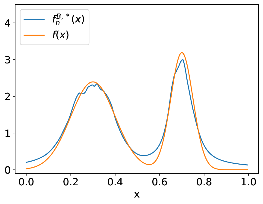
(a) BRDDE

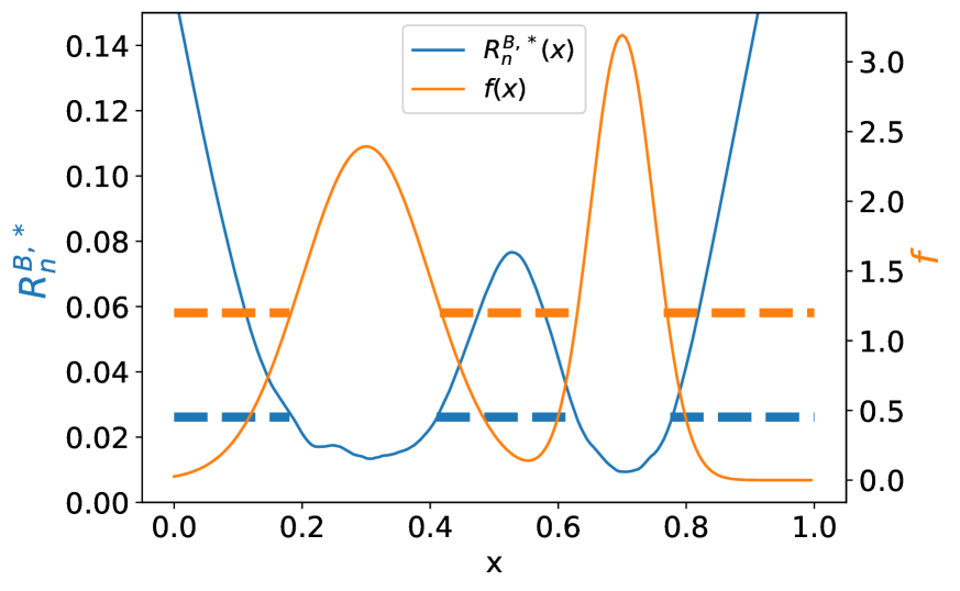
(b) Bagged regularized $k$-distances

Figure 1: (a) plots the BRDDE and the underlying density function $0.4*\mathcal{N}(0.3,0.01)+0.6*\mathcal{N}(0.7,0.0025)$. (b) shows the correspondence between the upper-level set of bagged regularized $k$-distances $R_{n}^{B,*}$ and the lower-level set of the true density function $f$. The curves of $R_{n}^{B,*}$ and $f$ are plotted in blue and orange, respectively. The upper-level set of $R_{n}^{B,*}$ and the lower-level set of $f$ are marked by dashed lines in blue and orange, respectively.

Now, we present our anomaly detection algorithm, bagged regularized $k$-distances for anomaly detection (BRDAD). We first sort the data $D_{n}$ into the sequence $\{\widetilde{X}_{1},\ldots,\widetilde{X}_{n}\}$ using their bagged regularized $k$-distances in descending order, i.e. $R_{n}^{B,*}(\widetilde{X}_{1})\geq\cdots\geq R_{n}^{B,*}(\widetilde{X}_{n})$. Given the pre-specified number of anomalies $m$, the first $m$ instances in the sorted sequence are considered the $m$ anomalies. The complete procedure of our BRDAD algorithm is presented in Algorithm 2.

Input: Data $D=\{X_{1},\cdots,X_{n}\}$; Number of anomalies $m$;

    Bagging rounds $B$; Subsampling size $s$;

for $b\in[B]$ do

       Sub-sample $s$ instances as $D_{s}^{b}$ from $D_{n}\setminus\bigcup_{i=1}^{b-1}D_{s}^{i}$ without replacement;

       Compute the weight $w^{b,*}$ by (5).

       Compute the regularized $k$-distances $R^{b,*}_{s}(X_{i})$ by (7) for $1\leq i\leq n$.

end for

Compute the bagged regularized $k$-distances $R_{n}^{B,*}(X_{i})$ by (8) for $1\leq i\leq n$.

Sort the data $D_{n}=\{X_{1},\ldots,X_{n}\}$ as $\{\widetilde{X}_{1},\ldots,\widetilde{X}_{n}\}$ with bagged regularized $k$-distances in a descending order, i.e. $R_{n}^{B,*}(\widetilde{X}_{1})\geq\cdots\geq R_{n}^{B,*}(\widetilde{X}_{n})$.

Output: Anomalies $\{\widetilde{X}_{i}\}_{i=1}^{m}$.

Algorithm 2 Bagged Regularized $k$-Distances for Anomaly Detection (BRDAD)

As illustrated above, SRM mitigates the hyperparameter selection challenge in density estimation. According to the equivalence relationship in (10), BRDAD shares the same weights assigned to the nearest neighbors with that of BRDDE. Therefore, BRDAD reserves the advantages of BRDDE to address the sensitivity of the hyperparameter selection of distance-based methods for unsupervised anomaly detection.

3 Theoretical Results

In this section, we present theoretical results related to our BRDAD algorithm. We first introduce the Huber contamination model in Section 3.1, in which we can analyze the performance of the bagged regularized $k$-distances from a learning theory perspective. Then, we present the convergence rates of BRDDE and BRDAD in Section 3.2 and 3.3, respectively. Finally, we provide comments and discussions on our algorithms and theoretical results in 3.4. We also compare our theoretical findings on the convergences of both BRDDE and BRDAD with other nearest-neighbor-based methods in this section.

3.1 Huber Contamination Model

To measure the performance of BRDAD, we need to formalize the anomaly detection problem mathematically, which is stated in the following assumption.

Assumption 2 (Huber Contamination Model).

We assume that the data $D_{n}$ are $\mathrm{i.i.d.}$ drawn from a distribution $\mathrm{P}$ that follows the Huber contamination model, that is,

$$\mathrm{P}=(1-\Pi)\cdot\mathrm{P}_{0}+\Pi\cdot\mathrm{P}_{1},$$ (11)

where $\mathrm{P}_{0}$ and $\mathrm{P}_{1}$ are distributions of the normal and anomalous instances, and $\Pi\in(0,1)$ is the unknown proportion of contamination. We further assume that $\mathrm{P}_{0}$ has probability density function $f_{0}$ and $\mathrm{P}_{1}$ has the uniform distribution over $[0,1]^{d}$ with the density function $f_{1}$.

The Huber contamination model (HCM) has been commonly adopted in the literature on unsupervised anomaly detection, see e.g., [25, 41]. We assume that the normal instances and anomalies are $\mathrm{i.i.d.}$ from distributions $\mathrm{P}_{0}$ and $\mathrm{P}_{1}$, respectively. In the model (11), the constant $\Pi$ represents the proportion of anomalies in the data. A larger $\Pi$ implies more anomalies are contained in the data.

In the Huber contamination model, for every instance $X$ from $\mathrm{P}$, we can use a latent variable $Y\in\{0,1\}$ that indicates which distribution it is from. More specifically, $Y=0$ and $Y=1$ indicate that the instance is from the normal and the anomalous distribution, respectively. As a result, the anomaly detection problem can be converted into a bipartite ranking problem where instances are labeled positive or negative implicitly according to whether it is normal or not. Let $\widetilde{\mathrm{P}}$ represents the joint probability distribution of $\mathcal{X}\times\mathcal{Y}$. In this case, our learning goal is to learn a score function that minimizes the probability of mis-ranking a pair of normal and anomalous instances, i.e. that maximizes the area under the ROC curve (AUC). Therefore, we can study regret bounds for the AUC of the bagged regularized $k$-distances to evaluate its performance from the learning theory perspective. Let $r:\mathcal{X}\to\mathbb{R}$ be a score function to measure the anomalous of the instance, then the $\mathrm{AUC}$ of $r$ can be written as

$$\mathrm{AUC}(r)=\mathbb{E}\bigl{[}\boldsymbol{1}\{(Y-Y^{\prime})(r(X)-r(X^{\prime})>0)\}+\boldsymbol{1}\{r(X)=r(X^{\prime})\}/2|Y\neq Y^{\prime}\bigr{]},$$

where $(X,Y)$, $(X^{\prime},Y^{\prime})$ are assumed to be drawn $\mathrm{i.i.d.}$ from $\widetilde{\mathrm{P}}$. In other words, the $\mathrm{AUC}$ of $r$ is the probability that a randomly drawn anomaly is ranked higher than a randomly drawn normal instance by the score function $r$. According to the HCM in (11), the posterior probability function w.r.t. $\widetilde{\mathrm{P}}$ is formulated as

$$\eta(x):=\widetilde{\mathrm{P}}(Y=1|X=x)=\frac{\Pi f_{1}(x)}{(1-\Pi)f_{0}(x)+\Pi f_{1}(x)}=\Pi f(x)^{-1}.$$ (12)

Then, the optimal $\mathrm{AUC}$ is defined as

$$\mathrm{AUC}^{*}:=\sup_{r:\mathcal{X}\to\mathbb{R}}\mathrm{AUC}(r)=1-\frac{1}{2\Pi(1-\Pi)}\mathbb{E}_{X,X^{\prime}}\bigl{[}\min\bigl{(}\eta(X)(1-\eta(X^{\prime})),\eta(X^{\prime})(1-\eta(X)\bigr{)}\bigr{]},$$

where $\eta(x)$ is specified in (12). Finally, the $\mathrm{AUC}$ regret of a score function $r$ is defined as

$$\mathrm{Reg}^{\mathrm{AUC}}(r):=\mathrm{AUC}^{*}-\mathrm{AUC}(r).$$

As is discussed in Section 2.2, our BRDAD is a density-based anomaly detection method. Therefore, in order to establish the convergence rates of BRDAD in the Huber contamination model, we can use the theoretical results related to the convergence rates of BRDDE in (9), which is presented in the next subsection.

3.2 Convergence Rates of BRDDE

The convergence rates of BRDDE are presented in the following Theorem.

Theorem 1.

Let Assumption 1 hold. Furthermore, let $w^{b,*}$ be defined as in (5). Finally, let $f$ be the underlying density function and $f_{n}^{B,*}$ be the BRDDE as in (9). If we choose

$$s_{n}\asymp(n/\log n)^{(d+1)/(d+2)}\quad\text{and}\quad B_{n}=n/s_{n}\asymp n^{1/(d+2)}(\log n)^{(d+1)/(d+2)},$$

then there exists an $N_{2}^{*}\in\mathbb{N}$, which will be specified in the proof, such that for all $n>N_{2}^{*}$, with probability $\mathrm{P}^{n}\otimes\mathrm{P}_{B}$ at least $1-1/n^{2}$, there holds

$$\int_{\mathcal{X}}|f_{n}^{B,*}(x)-f(x)|\,dx\lesssim n^{-1/(2+d)}(\log n)^{(d+3)/(d+2)}.$$

The convergence rate of the $L_{1}$-error of BRDDE in the above theorem matches the minimax lower bound established in [54] when the density function is Lipschitz continuous. Therefore, BRDDE attains the optimal convergence rates for density estimation. As a result, the SRM procedure in Section 2.3 turns out to be a promising approach for determining the weights of nearest neighbors for BWDDE.

Moreover, notice that the number of iterations required in the optimization problem (5) at each bagging round depends on the sub-sample size $s$. In Theorem 1, the choice of $s$ is significantly smaller than $n$, indicating that fewer iterations are required at each bagging round. This explains the computational efficiency of incorporating the bagging technique if parallel computation is employed. Further discussions on the complexity are presented in Section 4.3.

3.3 Convergence Rates of BRDAD

The next theorem provides the convergence rates for BRDAD.

Theorem 2.

Let Assumptions 1 and 2 hold. Furthermore, let $w^{b,*}$ be as in (5) and $R_{n}^{B,*}$ be the bagged regularized $k$-distances returned by Algorithm 2. If we choose

$$s_{n}\asymp(n/\log n)^{(d+1)/(d+2)}\quad\text{and}\quad B_{n}=n/s_{n}\asymp n^{1/(d+2)}(\log n)^{(d+1)/(d+2)},$$ (13)

then there exists an $N_{3}^{*}\in\mathbb{N}$, which will be specified in the proof, such that for all $n>N_{3}^{*}$, with probability $\mathrm{P}^{n}\otimes\mathrm{P}_{B}$ at least $1-1/n^{2}$, there holds

$$\mathrm{Reg}^{\mathrm{AUC}}(R_{n}^{B,*})\lesssim n^{-1/(2+d)}(\log n)^{(d+3)/(d+2)}.$$

The above theorem shows that up to a logarithm factor, the convergence rate of the AUC regret of BRDAD is of the order $\mathcal{O}(n^{-1/(d+2)})$ if we choose the number of bagging rounds $B$ and the subsample size $s$ according to (13). The parameter choices and the convergence rates in Theorem 2 coincide with that of BRDDE in Theorem 1. This is because our BRDAD is a density-based anomaly detection method based on BRDDE. Furthermore, the equivalence relationship as shown in (10) acts as a bridge that allows us to conduct the theoretical analysis of the AUC regret of $R_{n}^{B,*}$ from the statistical learning perspective.

3.4 Comments and Discussions

3.4.1 Comments on the Huber Contamination Model

In Assumption 2, we further assume that $\mathrm{P}_{1}$ follows the uniform distribution over the data space. This assumption is made implicitly in many well-known unsupervised anomaly detection methods such as [45, 32]. In fact, [45] points out that this assumption can be interpreted as a default uninformative prior to the anomalous distribution. This prior assumes the absence of abnormal modes and suggests that anomalies have an equal probability of occurring throughout the entire data space. When we have no prior knowledge about the anomalies, the uniform anomalous distribution is a reasonable assumption in unsupervised anomaly detection problems.

3.4.2 Comments on BRDDE

Comments on Sensitivity of Parameter Selection.

The literature extensively explores the concept of weighted $k$-nearest neighbors for density estimation. For instance, [37, 18, 16] have delved into standard $k$-NN density estimation. Additionally, [9] introduced the general weighted $k$-nearest neighbor density estimation, which associates weights with a specific probability measure. For a more comprehensive discussion on various nearest neighbor density estimation methods, the readers can refer to [10].

Given the unsupervised nature of density estimation, a notable challenge that these methods face is the sensitivity of parameter selection. To elaborate, the choice of the number of nearest neighbors $k$ significantly influences the performance of the density estimation. Choosing a smaller $k$ can result in an unstable density estimation, as it may be heavily affected by abnormal data points. Conversely, selecting a larger $k$ can yield a smoother estimation but with increased bias. Furthermore, commonly used parameter selection rules, such as the loss function for density estimation, e.g., average negative log-likelihood [15, 52] or leave-one-out cross-validation using the integrated mean squared error [48], are not practically applicable for nearest neighbor density estimations, particularly for high-dimensional datasets. Particularly, in the implementation of leave-one-out cross-validation, precise squared integrals of the candidate density estimations on $\mathbb{R}^{d}$ are required to be calculated to select the optimal parameters. Unfortunately, the squared integral of the weighted $k$-nearest neighbor density estimation on $\mathbb{R}^{d}$ does not have an explicit expression and thus has to be estimated by using the Monte Carlo method. However, when dealing with high-dimensional data, in order to ensure the accuracy of the estimation, a large number of samples are required to be drawn from $\mathbb{R}^{d}$ to compute the average of their density estimation squares. As a result, leave-one-out cross-validation is often infeasible when handling high-dimensional data.

To tackle the issue of parameter sensitivity in density estimation, we propose the SRM approach in Algorithm 1 and BRDDE in (9) in Section 2.3, which transforms unsupervised learning problem into convex optimization problems as in (5). As a result, the weights assigned to nearest neighbors can be efficiently solved based on the available data. Furthermore, the optimal convergence rate, as demonstrated in Theorem 1, implies that the SRM approach offers a valid way to determine the weights for BWDDE. This successfully mitigates the challenges associated with parameter selection in distance-based density estimation methods.

Comments on Convergence Rates.

We compare the theoretical results established for the weighted nearest neighbor density estimation with our theoretical results in this part. The consistency results for standard $k$-NN density estimation can be traced back to [37, 18]. First, [37] showed that when the density function $f$ is Lipstchitz continuous in a neighborhood of $x$ with $f(x)>0$ and $k_{n}$ is chosen satisfying $k_{n}\to\infty$ and $k/n^{2/(2+d)}\to 0$, the $k$-NN density estimation is asymptotically normal, i.e., $\sqrt{k}(f_{k}(x)-f(x))\stackrel{{\scriptstyle\mathcal{D}}}{{\to}}\mathcal{N}(0,1)$. Furthermore, [9] considered the general weighted $k$-NN density estimation. They showed the asymptotic normality holds when the density function $f$ is twice differentiable and $k_{n}$ is chosen as $k_{n}/n^{4/(4+d)}\to 0$. However, no finite sample generalization bounds of these weighted $k$-NN density estimations were established in these works. To deal with this issue, [16] established minimax optimal convergence rates for the $k$-NN density estimation when the density function is $\alpha$-Hölder smoothness. Recently, [54] analyzed the $L_{1}$ and $L_{\infty}$ convergence rates of $k$ nearest neighbor density estimations in two different cases depending on whether the probability density function has bounded support or not. Notably, all the theoretical results of these existing nearest-neighbor density estimations are based on the specific formulation of weights assigned to the nearest neighbors that are pre-determined by the user.

Different from the existing nearest neighbor density estimation in the literature, there exist no explicit formulations for the weights of the nearest neighbors in our BRDDE since they are solutions to the optimization problems (5) in Section 2.3. In this paper, by applying Bernstein’s concentration inequality which takes into account the variance information of the random variables within a learning theory framework [14, 44], we are able to obtain the upper and lower bounds for the weights induced by surrogate risk minimization (SRM) and thus establish the optimal convergence rates of our proposed BRDDE. The optimal rates verify the rationality of the SRM procedure in determining the weights of the nearest neighbors. Furthermore, the incorporated techniques such as approximation theory and empirical process theory [49, 31] yields our results on convergence rates are of type “with high probability”. Moreover, as discussed in the remark of Proposition 1, the inequality (1) covers the finite sample bounds of the empirical risk of both bagged $k$-nearest neighbor density estimation and bagged weighted $k$-nearest neighbor density estimation. By applying similar arguments as that in the proof of Theorem 2, we can obtain optimal convergence rates of these two density estimations by choosing sub-sampling size $s_{n}\asymp(n/\log n)^{(d+1)/(d+2)}$ and the number of nearest neighbors $k_{n}\asymp(n/\log n)^{1/(d+2)}$.

3.4.3 Comments on BRDAD

Our BRDAD retains the benefits of BRDDE through the equivalence equation (10) in Section 2.3 between the upper-level set of bagged regularized $k$-distance and the lower-level set of BRDDE. Since BRDDE effectively mitigates the challenges associated with parameter selection in distance-based methods for density estimation, BRDAD successfully addresses the sensitivity of parameter selection in those methods for unsupervised anomaly detection by utilizing the same weights of BRDDE. Moreover, to the best of our knowledge, we are the first to undertake a theoretical analysis of distance-based methods in the context of unsupervised anomaly detection. By converting the analysis of the bagged regularized $k$-distance into the analysis of the BRDDE from a statistical learning theory perspective [49], we can establish convergence rates for the AUC regret of bagged regularized $k$-distances under the Huber contamination model and mild assumptions regarding the density function in Theorem 2. Notably, our findings reveal that the convergence rates of the AUC regret for our method match the optimal convergence rates of $O(n^{-1/(d+2)})$ in density estimation, indicating the effectiveness of BRDAD.

In contrast, previous theoretical studies on distance-based methods for unsupervised anomaly detection did not transform the distance-based algorithms to the density estimations. As a result, no convergence rates were established for these methods. For instance, [46] introduced a rapid distance-based outlier detection via sampling and conducted a theoretical analysis to understand the effectiveness of the sampling-based approach compared to the conventional method based on $k$-nearest neighbors. More recently, [25] performed a statistical analysis of the distance-to-measure (DTM) for anomaly detection under the Huber contamination model and specific regularity assumptions on the distribution. They demonstrated that anomalies can be correctly identified with high probability. Since these prior works did not establish theoretical results on convergence rates of the AUC regret, their findings cannot be directly compared to our results.

4 Error and Complexity Analysis

We present the error analysis of the AUC regret and the complexity analysis of our algorithm in this section. In detail, in Section 4.1, we provide the error decomposition of the surrogate risk, which leads to the derivation of the surrogate risk in Proposition 1 in Section 2.3. Furthermore, in Section 4.2, we illustrate the three building blocks in learning the AUC regret, which indicates the way to establish the convergence rates of both BRDDE and BRDAD in Theorem 1 and 2 in Section 3.3. Finally, we analyze the time complexity of BRDAD, and illustrate the computational efficiency of BRDAD compared to other distance-based methods for anomaly detection in Section 4.3.

4.1 Error Analysis for the Surrogate Risk

In this section, we first provide the error decomposition for the density estimation BWDDE $f_{n}^{B}(x)$ in (1). Then, we present the upper bounds for these error terms.

Let the term $(I)$ be defined by

$$(I):=\frac{1}{\bigl{(}V_{d}R_{n}^{B}(x)\bigr{)}^{d}}\sum_{j=0}^{d-1}\biggl{(}\frac{1}{B}\sum_{b=1}^{B}\sum_{i=1}^{s}w_{i}^{b}(i/s)^{1/d}\biggr{)}^{j}\bigl{(}f(x)V_{d}R_{n}^{B}(x)\bigr{)}^{(d-1-j)/d}.$$ (14)

Then, using the triangle inequality and the equality

$$x^{d}-y^{d}=(x-y)\cdot\sum_{i=0}^{d-1}x^{i}y^{d-1-i},$$ (15)

we get

$$\bigl{|}f_{n}^{B}(x)-f(x)\bigr{|} =\frac{1}{V_{d}R_{n}^{B}(x)^{d}}\cdot\biggl{|}\biggl{(}\frac{1}{B}\sum_{b=1}^{B}\sum_{i=1}^{s}w_{i}^{b}(i/s)^{1/d}\biggr{)}^{d}-f(x)V_{d}R_{n}^{B}(x)^{d}\biggr{|}$$

$$=(I)\cdot\biggl{|}\frac{1}{B}\sum_{b=1}^{B}\sum_{i=1}^{s}w_{i}^{b}(i/s)^{1/d}-V_{d}^{1/d}f(x)^{1/d}R_{n}^{B}(x)\biggr{|}$$

$$\leq(I)\cdot\sum_{i=1}^{s}\sum_{b=1}^{B}(w_{i}^{b}/B)\cdot\Bigl{|}(i/s)^{1/d}-V_{d}^{1/d}f(x)^{1/d}R_{s,(i)}^{b}(x)\Bigr{|}.$$ (16)

If the terms $(II)$ and $(III)$ are respectively defined by

$$(II) :=\sum_{i=1}^{s}\sum_{b=1}^{B}(w_{i}^{b}/B)\cdot\Bigl{|}(i/s)^{1/d}-\mathrm{P}(B(x,R_{s,(i)}^{b}(x)))^{1/d}\Bigr{|},$$ (17)

$$(III) :=\sum_{i=1}^{s}\sum_{b=1}^{B}(w_{i}^{b}/B)\cdot\Bigl{|}\mathrm{P}(B(x,R_{s,(i)}^{b}(x)))^{1/d}-V_{d}^{1/d}f(x)^{1/d}R_{s,(i)}^{b}(x)\Bigr{|},$$ (18)

then by applying the triangle inequality to (4.1), we obtain the error decomposition

$$\bigl{|}f^{B}_{n}(x)-f(x)\bigr{|}\leq(I)\cdot(II)+(I)\cdot(III).$$ (19)

The following proposition provides the upper bounds for the error terms $(I)$, $(II)$, and $(III)$ in (14) and (17), and (18), respectively.

Proposition 2.

Let Assumption 1 hold. Furthermore, let $(I)$, $(II)$, and $(III)$ be as in (14) and (17), and (18), respectively. Moreover, let $k^{b}:=k(w^{b}):=\sup\{i\in[s]:w^{b}_{i}\neq 0\}$ with $w^{b}$ as in (5), $\underline{k}:=\min_{b\in[B]}k^{b}$, and $\overline{k}:=\max_{b\in[B]}k^{b}$. Finally, suppose that the following four conditions hold:

1. $s\gtrsim n^{d/(2+d)}(\log n)^{2/(2+d)}$ and $\displaystyle\sum_{i=1}^{c_{n}}w_{i}^{b}\lesssim\log s/k^{b}$ with $c_{n}\asymp\log n$ for $b\in[B]$;

2. $k^{b}\gtrsim\log s$, $\|w^{b}\|_{2}\gtrsim\bigl{(}k^{b}\bigr{)}^{-1/2}$, and $\displaystyle\sum_{i=1}^{s}i^{1/d}w_{i}^{b}\asymp\bigl{(}k^{b}\bigr{)}^{1/d}$ for $b\in[B]$;

3. $\underline{k}\asymp\overline{k}$ and $B\gtrsim\overline{k}\log n$;

4. $\displaystyle\max_{b\in[B]}w^{b}_{i}\leq V_{i}$ holds for $c_{n}<i\leq s$ and $\displaystyle\sum_{i=c_{n}}^{s}i^{1/d-1/2}V_{i}\lesssim\overline{k}^{1/d-1/2}$.

Then there exists an $N_{1}\in\mathbb{N}$, which will be specified in the proof, such that for all $n>N_{1}$ and $x$ satisfying $B(x,R_{s,(k^{b})}^{b}(x))\subset[0,1]^{d}$, $b\in[B]$, the following statements hold with probability $\mathrm{P}^{n}\otimes\mathrm{P}_{B}$ at least $1-1/n^{2}$:

1. $\lesssim\bigl{(}\overline{k}/s\bigr{)}^{-1/d}$;

2. $\lesssim(\overline{k}/s)^{1/d}\bigl{(}\log s/\underline{k}\bigr{)}+\bigl{(}\overline{k}/s\bigr{)}^{1/d}\bigl{(}\log s/(\overline{k}B)\bigr{)}^{1/2}$;

3. $\lesssim\bigl{(}\overline{k}/s\bigr{)}^{1/d}\bigl{(}\log s/\overline{k}\bigr{)}+(\overline{k}/s)^{2/d}$.

4.2 Learning the AUC Regret: Three Building Blocks

Recalling that the central concern in statistical learning theory is the convergence rates of learning algorithms under various settings. In Section 3.1, we show that when the probability distribution $\mathrm{P}$ follows the Huber contamination model in Assumption 2, we can use a latent variable $Y$ to indicate whether it is from the anomalous distribution. Moreover, the posterior probability in (12) implies that in HCM, anomalies can be identified by using the Bayes classifier with respect to the classification loss, resulting in the set of anomalies as

$$\mathcal{S}:=\{x\in\mathbb{R}^{d}:\eta(x)>1/2\}=\{x\in\mathbb{R}^{d}:\Pi f(x)^{-1}>1/2\}=\{x\in\mathbb{R}^{d}:f(x)<2\Pi\}.$$

Notice that this set is the lower-level set of the density function at the threshold $2\Pi$. $\mathcal{S}$ can be estimated by the lower-level set estimation of BRDDE as in (9), i.e., $\widehat{\mathcal{S}}:=\{x\in\mathbb{R}^{d}:f_{n}^{B,*}(x)<2\Pi\}$ with $f_{n}^{B,*}(x)$ as in (9). Recall that in Section 2.2, (10) implies that the lower-level set of $f_{n}^{B,*}(x)$ is equivalent to the upper-level set of $R_{n}^{B,*}(x)$. Therefore, if we choose $\theta=\bigl{(}2V_{d}\pi\bigr{)}^{-1/d}\bigl{(}(1/B)\sum_{b=1}^{B}\sum_{i=1}^{s}w_{i}^{b,*}(i/s)^{1/d}\bigr{)}^{d}$, then we have

$$\{x\in\mathbb{R}^{d}:R_{n}^{B,*}(x)\geq\theta\}=\{x\in\mathbb{R}^{d}:f_{n}^{B,*}(x)<2\Pi\}=\widehat{\mathcal{S}}.$$

This implies that the upper-level set of bagged regularized $k$-distances, i.e., $\{x\in\mathbb{R}^{d}:R_{n}^{B,*}(x)\geq\theta\}$, equals the estimation $\widehat{\mathcal{S}}$ with the properly chosen threshold. As a result, the unsupervised anomaly detection problem is converted to an implicit binary classification problem. Therefore, we are able to analyze the performance of $R_{n}^{B,*}(x)$ in anomaly detection by applying the analytical tools for classification. Since the posterior probability estimation is inversely proportional to the BRDDE as shown in (12) in Section 3.1, the problem of analyzing the posterior probability estimation can be further converted to analyzing the BRDDE. Therefore, it is natural and necessary to investigate the following three problems:

1. The finite sample bounds of the weight selection $w^{b,*}$ by solving SRM problems.

2. The convergence of the BRDDE as stated in Theorem 1, that is, whether $f_{n}^{B,*}$ converges to $f$ in terms of $L_{1}$-norm.

3. The convergence of AUC regret for $R_{n}^{B,*}$, i.e., whether the convergences of BRDDE $f_{n}^{B,*}$ imply the convergences of the AUC regret of $R_{n}^{B,*}$.

Figure 2: An illustration of the three building blocks for AUC regret. The left block stands for the consistency of AUC regret, the middle block denotes the consistency of the BRDDE, and the right block represents the statistical analysis of the SRM, corresponding to Problem (iii), (ii), and (i), respectively.

The above three problems form the foundations for conducting a learning theory analysis on bagged regularized $k$-distances and serve as three main building blocks. Notice that Problem (ii) is already provided in Theorem 1 in Section 3.2. Detailed explorations of the other two Problems (i) and (iii), will be expanded in the following subsections.

4.2.1 Analysis for the Surrogate Risk Minimization

In the following Proposition 3, we provide theoretical guarantees on the weights returned by the optimizations problem in (5), which solves Problem (i).

Proposition 3.

Let Assumption 1 hold. Furthermore, let $\overline{R}_{s,(i)}^{b}=\sum_{j=1}^{s}R_{s,(i)}^{b}(X_{j}^{b})/s$ be the average $i$-distance of the subset $D_{s}^{b}$ with $s\gtrsim n^{d/(2+d)}(\log n)^{2/(2+d)}$. Moreover, let $w^{b,*}$ be as in (5) and $k^{b,*}:=k(w^{b,*}):=\sup\{i\in[n]:w_{i}^{b,*}\neq 0\}$. Then there exists an $N_{2}\in\mathbb{N}$, which will be specified in the proof, such that for all $n>N_{2}$ and all $b\in[B]$, the following statements hold with probability $\mathrm{P}^{n}\otimes\mathrm{P}_{B}$ at least $1-1/n^{2}$:

1. $k^{b,*}\asymp s^{2/(2+d)}(\log s/B)^{d/(2+d)}$;

2. $\displaystyle\sum_{i=1}^{s}w_{i}^{b,*}i^{1/d}\asymp(k^{b,*})^{1/d}$;

3. $\displaystyle\sum_{i=1}^{s}w_{i}^{b,*}\overline{R}_{\mathrm{s},(i)}^{b}\asymp(k^{b,*}/s)^{1/d}$ and $\|w^{b,*}\|_{2}\asymp(k^{b,*})^{-1/2}$.

4.2.2 Analysis for the AUC Regret

Problem (iii) in the left block of Figure 2 is solved by the next proposition, which shows that the problem of bounding the AUC regret of the bagged regularized $k$-distances can be converted to the problem of bounding the $L_{1}$-error of the BRDDE.

Proposition 4.

Let Assumptions 1 and 2 hold. Furthermore, let $f$ be the underlying density function of the probability distribution $\mathrm{P}$. Moreover, let $R_{n}^{B,*}$ be the bagged regularized $k$-distances as in (8) and the density estimation $f_{n}^{B,*}(x)$ be the BRDDE as in (9). Finally, suppose that there exists a constant $c\geq 0$ such that $\|f_{n}^{B,*}\|_{\infty}\geq c$. Then we have

$$\mathrm{Reg}^{\mathrm{AUC}}(R_{n}^{B,*})\displaystyle\lesssim\int_{\mathcal{X}}\bigl{|}f_{n}^{B,*}(x)-f(x)\bigr{|}dx.$$

4.3 Complexity Analysis

To deal with the efficiency issue in distance-based methods for anomaly detection when dealing with large-scale datasets, [53] proposed the iterative subsampling, i.e., for each test sample, they first randomly select a portion of data and then compute the $k$-distance over the subsamples. They provided a probabilistic analysis of the quality of the subsampled distance compared to the $k$-distance over the whole dataset. Furthermore, [46] proposed the one-time sampling for the computation of the $k$-distances over the dataset for all test samples, which is shown to be more efficient than the iterative sampling. Although these sub-sampling methods improve computational efficiency, these distance-based methods fail to comprehensively utilize the information in the dataset since a large portion of samples are dropped out. By contrast, the bagging technique incorporated in our BRDAD not only addresses the efficiency issues when dealing with large-scale datasets but also maintains the ability to make full use of the data. In the following, we conduct a complexity analysis for BRDAD in detail to show the computational efficiency of BRDAD.

As a commonly-used algorithm, $k$-d tree [23] is used in NN-based methods to search the nearest neighbors. Given $n$ data points with dimension $d$, [23] showed that constructing a $k$-$d$ tree takes $\mathcal{O}(nd\log n)$ time and searching for $k$ nearest points takes $\mathcal{O}(k\log n)$ time. In what follows, we analyze the time complexities of the construction and search stages in BRDAD to demonstrate the advantage of bagging in reducing the time complexity of BRDAD.

1. In the construction stage, our BRDAD algorithm builds a $k$-$d$ tree with $s$ data points at each bagging round, which requires the construction time $\mathcal{O}(dn^{(1+d)/(d+2)}(\log n)^{1/(d+2)})$ if parallelism is applied. By contrast, without bagging $\mathcal{O}(nd\log n)$ is required for the construction of a $k$-$d$ tree. Therefore, bagging helps reduce the time complexity of the construction stage.

2. In the search stage, the time complexity of regularized $k$-distances at each bagging round is mainly made up of two parts: calculating the average $k$-distances and solving the SRM problem. In the first part, the query of $k^{b,*}=k(w^{b,*})$ neighbors takes $\mathcal{O}(k^{b,*}\log n)$ time. As for the second part, Theorem 3.3 in [7] shows that Algorithm 1 finds the solution with an $\mathcal{O}(k^{b,*})$ running time. Consequently, the search stage takes at most $\mathcal{O}(k^{b,*}\log n)$ time. When bagging is applied with parallelism, the time complexity of the search stage is $\mathcal{O}(n^{1/(d+2)}(\log n)^{(d+1)/(d+2)})$ by Theorem 2. However, when bagging is not applied, the time complexity of the search stage is $\mathcal{O}(n^{2/(d+2)}(\log n)^{(2+2d)/(2+d)})$ by Proposition 3. Therefore, bagging also helps reduce the time complexity of the search stage.

In summary, the bagging technique can enhance computational efficiency considerably when parallel computation is fully employed.

For popular distance-based anomaly detection methods such as standard $k$-NN and DTM [25], their time complexities are also mainly composed of constructing a $k$-$d$ tree and searching for $k$ nearest points. If $k$ is chosen to be the optimal order $\mathcal{O}(n^{2/(d+2)}(\log n)^{d/(d+2)})$ for the standard $k$-NN density estimation, the construction stage takes $\mathcal{O}(nd(\log n)^{(2d+2)/(d+2)})$ time and the search stage takes $\mathcal{O}(n^{2/(2+d)}(\log n)^{(2d+2)/(d+2)})$ time. As for another distance-based method LOF, besides constructing a $k$-$d$ tree and searching for $k$ nearest points, LOF has an additional step in calculating the score for all the samples, whose time complexity is $\mathcal{O}(n)$, as discussed in [11]. An easy comparison finds that the time complexities of all these methods are significantly larger than those of our BRDAD, since the time complexities of the construction stage (i) and the search stage (ii) of BRDAD are merely $\mathcal{O}(dn^{(1+d)/(d+2)}(\log n)^{1/(d+2)})$ and $\mathcal{O}(n^{1/(d+2)}(\log n)^{(d+1)/(d+2)})$, respectively.

5 Experiments

In this section, we conduct numerical experiments to illustrate our proposed BRDAD. In Section 5.1, we conduct synthetic data experiments on density estimation, including the convergence of Algorithm 1 and the convergences of the surrogate risk and mean absolute error of BRDDE. The sensitivity of the parameter selection is analyzed experimentally in this subsection as well. In Section 5.2, we conduct experiments on real-world benchmarks for anomaly detection. Specifically, we evaluate our proposed BRDAD by comparing it with various methods and conduct parameter analysis of BRDAD. Our results empirically demonstrate that bagging can improve the performance of our algorithm. Furthermore, we conduct experiments to analyze the sensitivity of the parameter selection in existing distance-based methods.

5.1 Synthetic Data Experiments on Density Estimation

In Section 5.1.1, we empirically validate the convergence of Algorithm 1 for SRM problem (5), i.e., the surrogate risk monotonically decreases with the progress of iteration until the algorithm meets the stopping criterion. Then, in Section 5.1.2, from an empirical perspective, we demonstrate the convergences of the surrogate risk and the mean absolute error of BRDDE as the sample size $n$ increases. Finally, in Section 5.1.3, we conduct simulations to show that our BRDDE addresses the sensitivity of parameter selection in density estimation.

5.1.1 Convergence of Algorithm 1

The SRM problem (5) is a convex optimization problem [7], whose empirical solution method is to add nearest neighbors in a greedy manner based on their distance from $x$ until a stopping criterion is met, as presented in Algorithm 1. In the following, we empirically validate the convergence of our solution that was developed in [7, 19, 43]. To this end, we draw 1000 sample points from $\mathcal{N}(0,1)$ and apply Algorithm 1 with $B=1$. At each iteration of the loop in Algorithm 1, we compute the values of $A$ and $w^{b,*}$ based on the $\mu_{k}$ obtained for each iteration $k$, and then calculate the corresponding surrogate risk based on $w^{b,*}$.

As seen in Figure 3(a), the surrogate risk monotonically decreases with the number of nearest neighbors $k$ increases, until it reaches the stopping criterion, which empirically shows the convergence of the Algorithm 1.

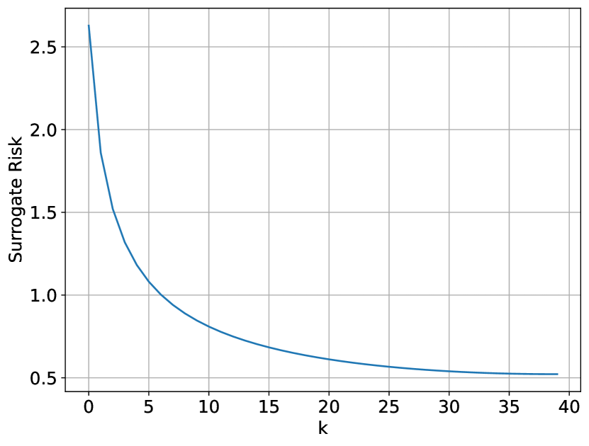
(a) Convergence of Algorithm 1

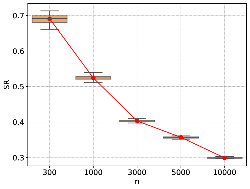
(b) Convergence of SR

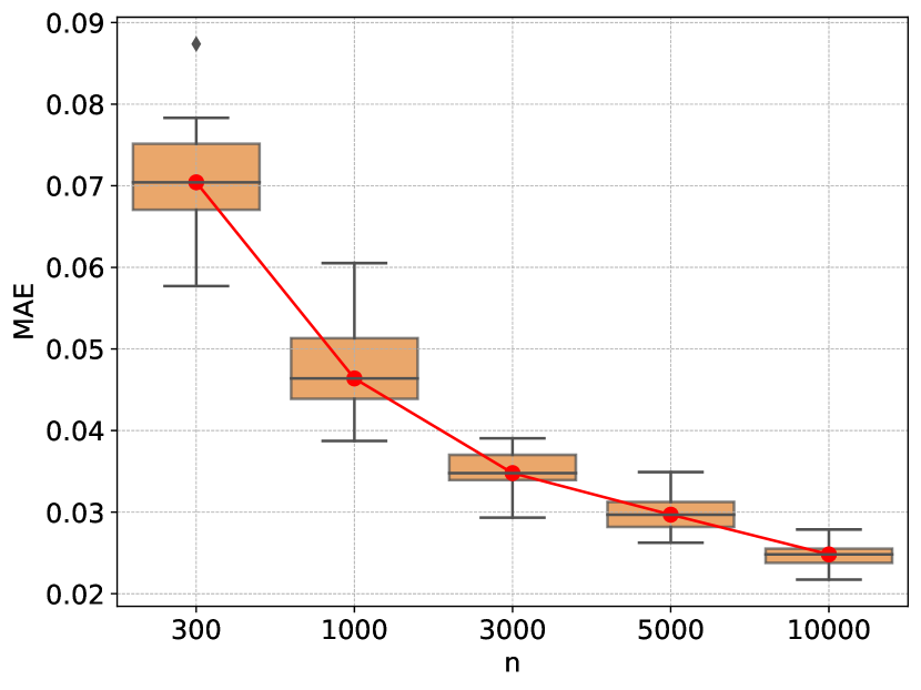
(c) Convergence of MAE

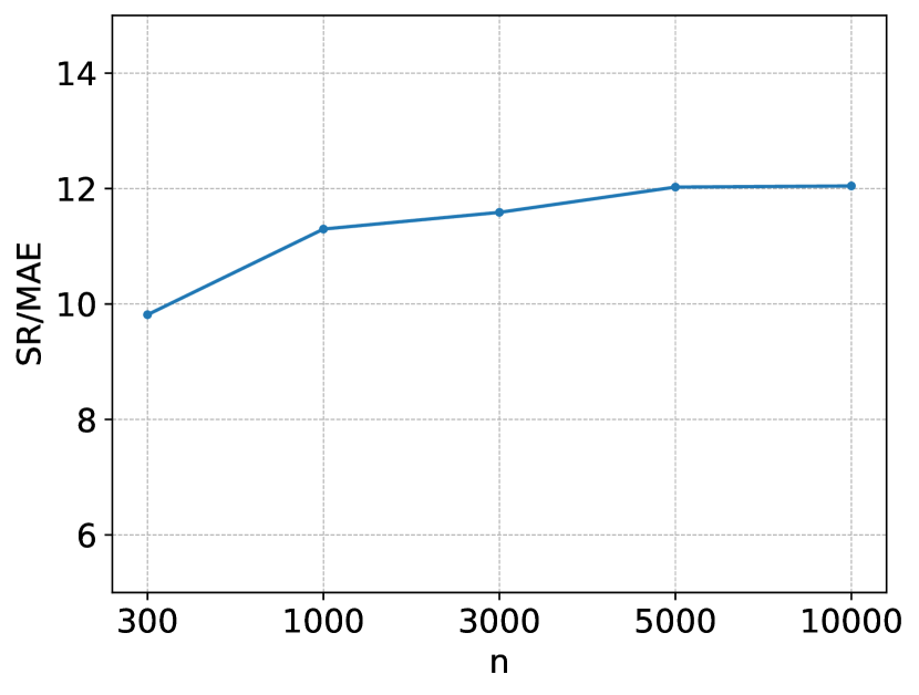
(d) Ratio of SR to MAE

Figure 3: (a) shows the convergence of Algorithm 1. (b)(c)(d) show that SRM leads to the convergences of both surrogate risk (SR) and mean absolute error (MAE). Furthermore, as the sample size $n$ increases, the ratio of SR to MAE becomes stable, indicating similar convergence behaviors for both SR and MAE by applying Algorithm 1.

5.1.2 Convergence of Surrogate Risk and MAE of BRDDE

In the following, we empirically show that the convergence of the surrogate risk (SR) has a similar behavior to the convergence of the mean absolute error (MAE) of BRDDE. To this end, we sample $n$ data points from the $\mathcal{N}(0,1)$ distribution, where the sample size $n$ is set to be ${300,1000,3000,5000,10000}$ for training purposes. Then we compute SR for each $n$ by applying Algorithm 1 with $B=1$. Furthermore, we randomly sample another $10,000$ instances to calculate MAE as in (2) to measure the performance of our BRDDE. We repeat these experiments 20 times for each sample size $n$. The results in Figure 3(b) show that as the sample size $n$ increases, the SR exhibits a monotonically decreasing trend, whereas the results in Figure 3(c) show a similar convergence pattern for the MAE. Moreover, we plot the ratio of SR and MAE for each sample size $n$ in Figure 3(d). Figure 3(d) shows that the ratio of SR and MAE is stable when the sample size $n$ is larger than $3000$, which illustrates that the convergence behaviors of both SR and MAE are similar by applying Algorithm 1.

5.1.3 Sensitivity Analysis of Choosing the Hyper-parameter $k$

We provide an illustrative example on a synthetic dataset to demonstrate the sensitivity of choosing the hyper-parameter $k$ in distance-based density estimation methods, including the $k$-NN density estimation ($k$-NN) and the weighted $k$-NN density estimation (WkNN) [9] taking the uniform distribution as the probability measure.

To this end, we generate 1000 data points to train the density estimation and an additional 10000 points to compute the MAE from a Gaussian mixture model with the density function $0.5\times\mathcal{N}(0.3,0.01)+0.5\times\mathcal{N}(0.7,0.0025)$. The hyper-parameter $k$ was varied from 3 to 500 to observe its effect on the MAE for both $k$-NN and WkNN.

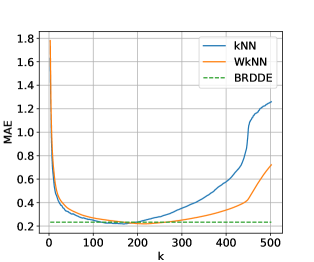
Figure 4: Illustration of the sensitivity of choosing the parameter $k$ in distance-based density estimation algorithms ($k$-NN, WkNN) and how the proposed density estimation BRDDE avoids the sensitivity of choosing $k$.

In Figure 4, we plot the MAE results for the $k$-NN and WkNN algorithms using blue and orange lines, respectively, showing that the performance of distance-based density estimations can be heavily dependent on the choice of the hyper-parameter $k$, with only a narrow range of $k$ values leading to optimal results. In contrast, our proposed estimator BRDDE avoids the sensitivity problem of choosing $k$. The green dashed line in Figure 4 visualizes the MAE performance of BRDDE, showing that BRDDE can achieve the optimal performance of the other two density estimations without requiring the fine-tuning of $k$.

5.2 Real-world Data Experiments on Anomaly Detection

5.2.1 Dataset Descriptions

To provide an extensive experimental evaluation, we use the latest anomaly detection benchmark repository named ADBench established by [26]. The repository includes 47 tabular datasets, ranging from 80 to 619326 instances and from 3 to 1555 features. We provide the descriptions of these datasets in the Table 1.

Table 1: Descriptions of ADBench Datasets

Number	Data	# Samples	# Features	# Anomaly	% Anomaly	Category
1	ALOI	49534	27	1508	3.04	Image
2	annthyroid	7200	6	534	7.42	Healthcare
3	backdoor	95329	196	2329	2.44	Network
4	breastw	683	9	239	34.99	Healthcare
5	campaign	41188	62	4640	11.27	Finance
6	cardio	1831	21	176	9.61	Healthcare
7	Cardiotocography	2114	21	466	22.04	Healthcare
8	celeba	202599	39	4547	2.24	Image
9	census	299285	500	18568	6.20	Sociology
10	cover	286048	10	2747	0.96	Botany
11	donors	619326	10	36710	5.93	Sociology
12	fault	1941	27	673	34.67	Physical
13	fraud	284807	29	492	0.17	Finance
14	glass	214	7	9	4.21	Forensic
15	Hepatitis	80	19	13	16.25	Healthcare
16	http	567498	3	2211	0.39	Web
17	InternetAds	1966	1555	368	18.72	Image
18	Ionosphere	351	32	126	35.90	Oryctognosy
19	landsat	6435	36	1333	20.71	Astronautics
20	letter	1600	32	100	6.25	Image
21	Lymphography	148	18	6	4.05	Healthcare
22	magic.gamma	19020	10	6688	35.16	Physical
23	mammography	11183	6	260	2.32	Healthcare
24	mnist	7603	100	700	9.21	Image
25	musk	3062	166	97	3.17	Chemistry
26	optdigits	5216	64	150	2.88	Image
27	PageBlocks	5393	10	510	9.46	Document
28	pendigits	6870	16	156	2.27	Image
29	Pima	768	8	268	34.90	Healthcare
30	satellite	6435	36	2036	31.64	Astronautics
31	satimage-2	5803	36	71	1.22	Astronautics
32	shuttle	49097	9	3511	7.15	Astronautics
33	skin	245057	3	50859	20.75	Image
34	smtp	95156	3	30	0.03	Web
35	SpamBase	4207	57	1679	39.91	Document
36	speech	3686	400	61	1.65	Linguistics
37	Stamps	340	9	31	9.12	Document
38	thyroid	3772	6	93	2.47	Healthcare
39	vertebral	240	6	30	12.50	Biology
40	vowels	1456	12	50	3.43	Linguistics
41	Waveform	3443	21	100	2.90	Physics
42	WBC	223	9	10	4.48	Healthcare
43	WDBC	367	30	10	2.72	Healthcare
44	Wilt	4819	5	257	5.33	Botany
45	wine	129	13	10	7.75	Chemistry
46	WPBC	198	33	47	23.74	Healthcare
47	yeast	1484	8	507	34.16	Biology

5.2.2 Methods for Comparison

We conduct experiments on the following anomaly detection algorithms.

• BRDAD is our proposed algorithm with details listed in Algorithm 2. There are two hyper-parameters, including the bagging rounds $B$ and the subsampling size $s$. For the sake of convenience, we fix $s=[n/B]$ so the bagging rounds $B$ is the only one hyper-parameter and is set to be $B=5$ as default.

• Distance-To-Measure (DTM) [25] is a distance-based algorithm which employs a generalization of the $k$ nearest neighbors named “distance-to-measure”. We use the author’s implementation. As suggested by the authors, the number of neighbors $k$ is fixed to be $k=0.03\times\text{sample size}$.

• $k$-Nearest Neighbors ($k$-NN) [39] is a distance-based algorithm that uses the distance of a point from its $k$-th nearest neighbor to distinguish anomalies. We use the implementation of the Python package PyOD with its default parameters.

• Local Outlier Factor (LOF) [11] is a distance-based algorithm that measures the local deviation of the density of a given data point with respect to its neighbors. We also use PyOD with its default parameters.

• Partial Identification Forest (PIDForest) [24] is a forest-based algorithm that computes the anomaly score of a point by determining the minimum density of data points across all subcubes partitioned by decision trees. We use the authors’ implementation with the number of trees $T=50$, the number of buckets $B=5$, and the depth of trees $p=10$ suggested by the authors.

• Isolation Forest (iForest) [33] is a forest-based algorithm that works by randomly partitioning features of the data into smaller subsets and distinguishing between normal and anomalous points based on the number of “splits” required to isolate them, with anomalies requiring fewer splits. We use the implementation of the Python package PyOD with its default parameters.

• One-class SVM (OCSVM) [42] is a kernel-based algorithm which tries to separate data from the origin in the transformed high-dimensional predictor space. We also use PyOD with its default parameters.

Note that as BRDAD, iForest, and PIDForest are randomized algorithms, we repeat these three algorithms for 10 runs and report the averaged AUC performance. DTM, $k$-NN, LOF, and OCSVM are deterministic, and hence we report a single AUC number for them.

5.2.3 Experimental Results

Table 2: Experimental Comparisons on ADBench Datasets

	BRDAD	DTM	$k$-NN	LOF	PIDForest	iForest	OCSVM
ALOI	0.5473	0.5440	0.6942	0.7681	0.5061	0.5411	0.5326
annthyroid	0.6516	0.6772	0.7343	0.7076	0.8781	0.8138	0.5842
backdoor	0.8425	0.9216	0.6682	0.7135	0.6965	0.7238	0.8465
breastw	0.9883	0.9799	0.9765	0.3907	0.9750	0.9871	0.8052
campaign	0.6826	0.6908	0.7202	0.5366	0.7945	0.7182	0.6630
cardio	0.9142	0.8879	0.7330	0.6372	0.8258	0.9271	0.9286
Cardiotocography	0.6302	0.6043	0.5449	0.5705	0.5587	0.6973	0.7872
celeba	0.6130	0.6929	0.5666	0.4332	0.6732	0.6955	0.6962
census	0.6402	0.6435	0.6465	0.5501	0.5543	0.6116	0.5336
cover	0.9298	0.9277	0.7961	0.5262	0.8065	0.8784	0.9141
donors	0.7870	0.8000	0.6117	0.5977	0.6945	0.7810	0.7323
fault	0.7591	0.7587	0.7286	0.5827	0.5437	0.5714	0.5074
fraud	0.9551	0.9583	0.9342	0.4750	0.9489	0.9493	0.9477
glass	0.7993	0.8688	0.8640	0.8114	0.7913	0.7933	0.4407
Hepatitis	0.6954	0.6303	0.6745	0.6429	0.7186	0.6944	0.6418
http	0.9946	0.0507	0.2311	0.3550	0.9870	0.9999	0.9949
InternetAds	0.7274	0.7063	0.7110	0.6485	0.6754	0.6913	0.6890
Ionosphere	0.9113	0.9237	0.9259	0.8609	0.6820	0.8493	0.7395
landsat	0.6176	0.6184	0.5773	0.5497	0.5245	0.4833	0.3660
letter	0.8426	0.8417	0.8950	0.8872	0.6636	0.6318	0.4843
Lymphography	0.9988	0.9965	0.9988	0.9953	0.9656	0.9993	0.9977
magic.gamma	0.8228	0.8214	0.8323	0.6712	0.7252	0.7316	0.5947
mammography	0.8156	0.8301	0.8424	0.7398	0.8453	0.8592	0.8412
mnist	0.8335	0.8630	0.8041	0.6498	0.5366	0.7997	0.8204
musk	0.7583	0.9987	0.6604	0.4271	0.9997	0.9995	0.8094
optdigits	0.3912	0.5474	0.4189	0.5831	0.8248	0.6970	0.5336
PageBlocks	0.8889	0.8859	0.7813	0.7345	0.8154	0.8980	0.8903
pendigits	0.8913	0.9581	0.7127	0.4821	0.9214	0.9515	0.9354
Pima	0.7291	0.7224	0.7137	0.5978	0.6842	0.6803	0.6022
satellite	0.7449	0.7375	0.6489	0.5436	0.7122	0.7043	0.5972
satimage-2	0.9991	0.9991	0.9164	0.5514	0.9919	0.9935	0.9747
shuttle	0.9804	0.9442	0.6317	0.5239	0.9885	0.9968	0.9823
skin	0.7570	0.7177	0.5881	0.5756	0.7071	0.6664	0.4857
smtp	0.8476	0.8854	0.8953	0.9023	0.9203	0.9077	0.7674
SpamBase	0.5687	0.5663	0.4977	0.4581	0.6941	0.6212	0.5251
speech	0.4834	0.4810	0.4832	0.5067	0.4739	0.4648	0.4639
Stamps	0.8980	0.8594	0.8362	0.7269	0.8883	0.8911	0.8179
thyroid	0.9353	0.9470	0.9508	0.8075	0.9687	0.9771	0.8437
vertebral	0.3236	0.3663	0.3768	0.4208	0.2857	0.3515	0.3852
vowels	0.9489	0.9667	0.9797	0.9443	0.7817	0.7590	0.5507
Waveform	0.7783	0.7685	0.7457	0.7133	0.7263	0.7144	0.5393
WBC	0.9972	0.9930	0.9925	0.8399	0.9904	0.9959	0.9967
WDBC	0.9841	0.9773	0.9782	0.9796	0.9916	0.9850	0.9877
Wilt	0.3138	0.3545	0.4917	0.5394	0.5012	0.4477	0.3491
wine	0.8788	0.4277	0.4992	0.8756	0.8221	0.7987	0.6941
WPBC	0.5188	0.5101	0.5208	0.5184	0.5283	0.4942	0.4743
yeast	0.3717	0.3876	0.3936	0.4571	0.4019	0.3964	0.4141
Rank Sum	147.5	162	192.5	243	186	159	226
Num. No. 1	11	8	5	5	9	6	3

Table 2 shows the performances of seven methods on the ADBench anomaly detection benchmarks under the AUC metric. We also provide the rank sum and the number of top-one performances for each algorithm in the last two rows of the table. A smaller rank sum and a larger number of top-one performances are better. We present the exceptional performance of the BRDAD algorithm across two evaluation metrics in the table. Specifically, in terms of the rank sum metric, the BRDAD algorithm achieves a remarkable minimum value of 147.5, significantly lower than the other comparative methods. Meanwhile, DTM and iForest obtain scores of 162 and 159 each. Looking at the perspective of achieving first place in multiple datasets, BRDAD attains the top position in 11 out of 47 tabular datasets, whereas PIDForest and DTM are followed by 9 out of 47 and 8 out of 47, respectively. Considering both the rank sum metric and the number of first-place rankings, our BRDAD algorithm demonstrates outstanding performance. It not only surpasses previous distance-based methods in quantity but also holds its ground against forest-based methods.

• On the one hand, the BRDAD algorithm outperforms distance-based methods like DTM and $k$-NN in comparison. For instance, on the satellite dataset, while DTM achieves a high score of 0.7375, our BRDAD algorithm achieves an even better score of 0.7449. Moreover, on the InternetAds dataset, despite $k$-NN scoring 0.7177, the BRDAD algorithm achieves a further improvement of 0.7274.

• On the other hand, in datasets where some distance-based methods perform poorly but forest-based methods excel, such as the Stamps dataset and wine dataset, the BRDAD algorithm also showcases its superiority. On the Stamps dataset, while DTM and $k$-NN have AUC scores of 0.8594 and 0.8362 respectively, existing forest-based methods like PIDForest and iForest achieve impressively high AUC scores of 0.8883 and 0.8911. Surprisingly, BRDAD, being a distance-based method, attains an AUC of 0.8980 on this dataset. Similarly, on the wine dataset, the forest-based methods PIDForest and iForest achieve AUC scores as high as 0.8221 and 0.7987, respectively, whereas the distance-based methods DTM and $k$-NN have AUC scores of only 0.4277 and 0.4992. Unexpectedly, as a distance-based method, the BRDAD algorithm also exhibits commendable performance on this dataset, reaching the highest AUC of 0.8788.

The above results empirically show the preponderance of BRDAD over the latest distance-based and forest-based anomaly detection algorithms.

5.2.4 Parameter Analysis

In this section, we conduct parameter analysis of the bagging rounds $B$ in BRDAD on ADBench datasets. To this end, we consider $B\in\{1,2,5,10,20\}$, compare with the methods as in Section 5.2.2, and record the rank sum metric and the number of first-place rankings for BRDAD with different $B$ respectively.

Table 3: Experimental Comparisons for BRDAD with different $B$ on ADBench Datasets

	$B=1$	$B=2$	$B=5$	$B=10$	$B=20$
Rank Sum	151.5	152.5	147.5	146.5	151.5
Num. No. 1	9	11	11	9	10

Table 3 shows that the rank sum metric exhibits superior performance when $B$ is set to 5 or 10 compared to other $B$ values, whereas $B$ shows little difference in the number of first-place rankings, suggesting that the BRDAD algorithm performs better when $B$ is either 5 or 10, as opposed to choosing smaller or larger $B$ values. Therefore, it is recommended to select an empirical value of $B$ as 5 or 10. Moreover, considering both the rank sum metric and the number of first-place rankings in Tables 2 and 3, our BRDAD with these five $B$ outperforms other comparing algorithms, especially when $B=1$, i.e., the non-bagged version of BRDAD, which demonstrates the effectiveness of the BRDAD algorithm with the bagging technique.

5.2.5 Sensitivity Analysis of $k$ for Parameter Selection

In this part, we provide a two-dimensional illustrative example to demonstrate the challenge of selecting $k$ for anomaly detection, where two features are independent and identically distributed variables following $0.4*\mathcal{N}(0.3,0.01)+0.6*\mathcal{N}(0.7,0.0025)$.

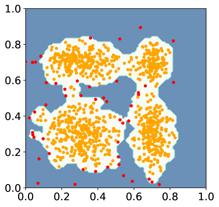
(a) $k=5$, DTM

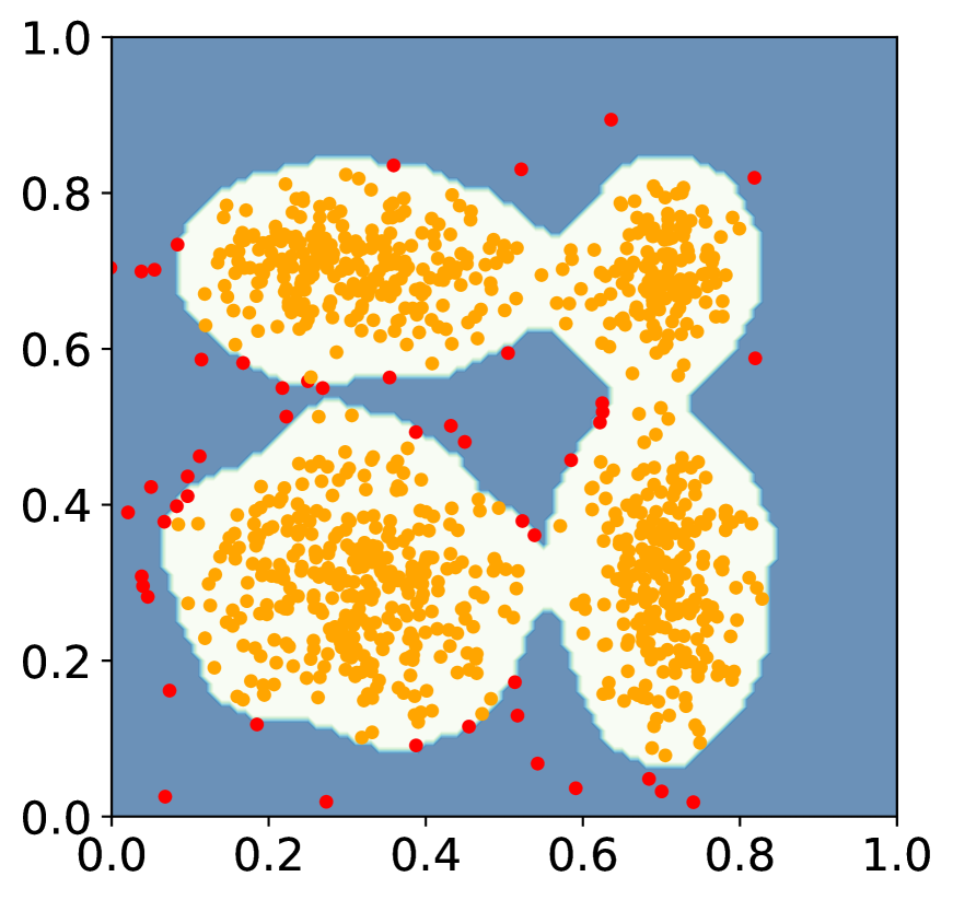
(b) $k=20$, DTM

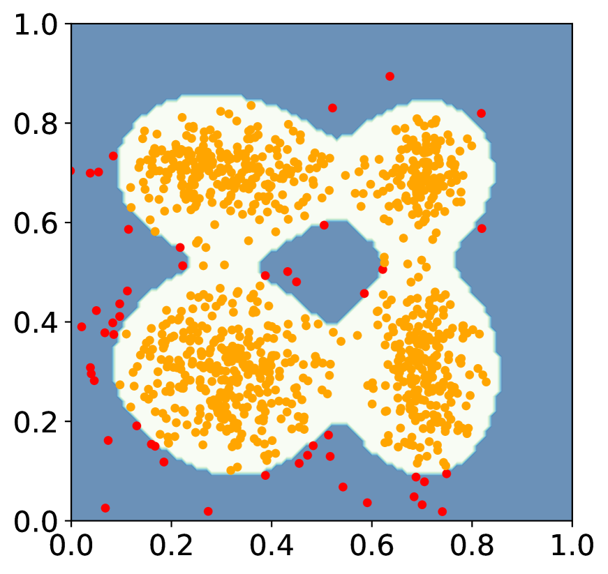
(c) $k=100$, DTM

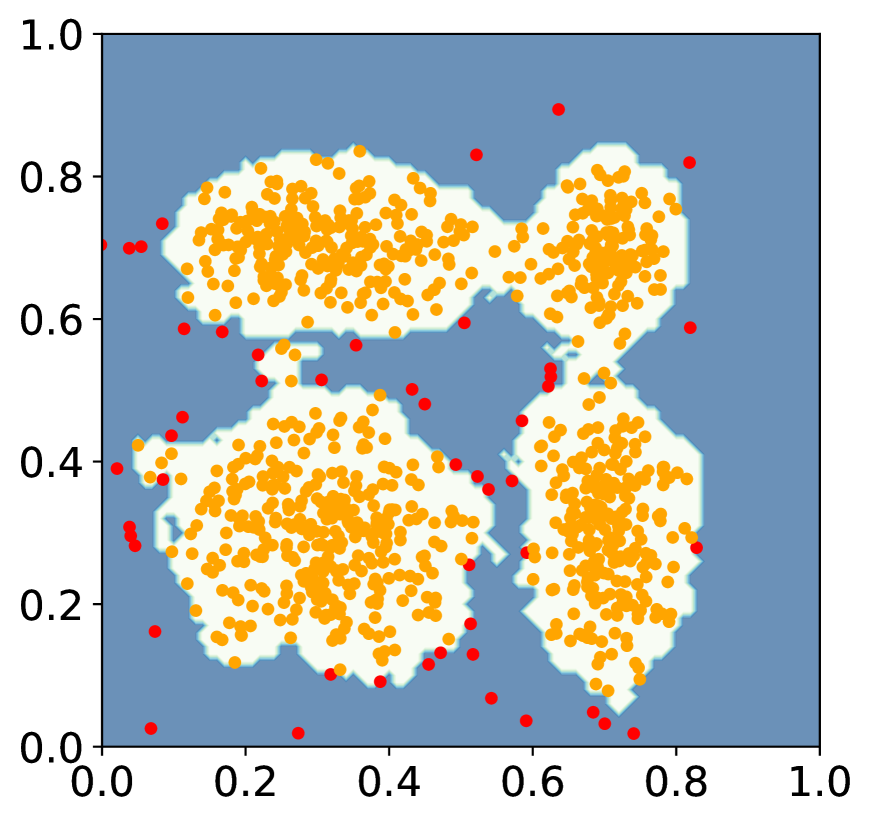
(d) $k=5$, $k$-NN

(e) $k=20$, $k$-NN

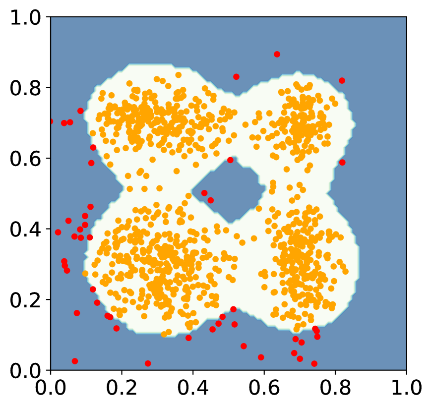
(f) $k=100$, $k$-NN

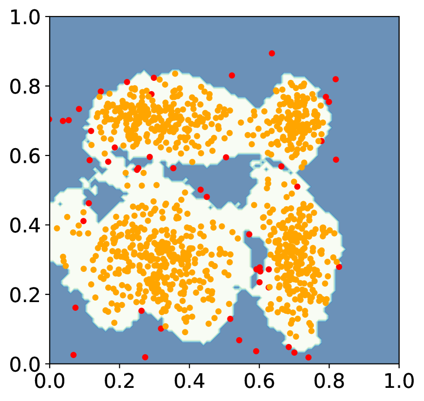
(g) $k=10$, LOF

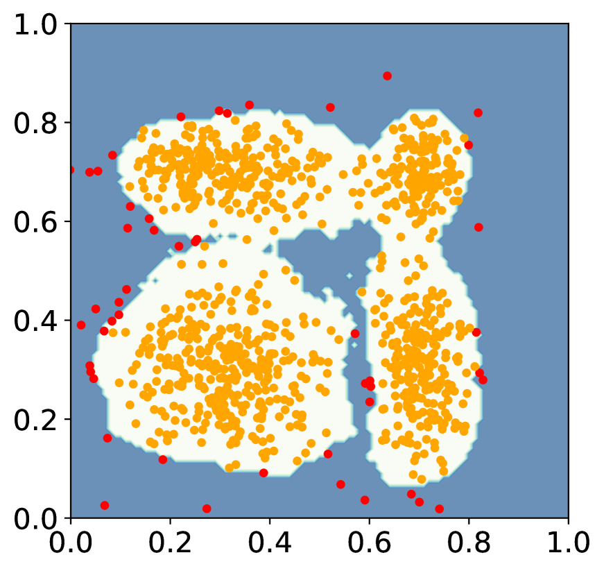
(h) $k=30$, LOF

(i) $k=100$, LOF

Figure 5: The illustration of sensitivity of parameter $k$ in distance-based methods $k$-NN, DTM, and LOF. We provide scatter plots for a training dataset of size $n=1000$, where the number of anomalies $m$ is fixed at $50$. Anomalies detected with a contamination ratio of $0.05$ are displayed in the blue area, while normal points are displayed in the white area.

In Figure 5, we can clearly find that the anomalies are distributed around the data and in the central area of the data. On the one hand, a small $k$ ($k=5$ for DTM and $k$-NN and $k=10$ for LOF) makes $k$-distance overfit the distribution, resulting in broken and irregular boundaries of anomalies. On the other hand, a larger $k$ ($k=100$ for DTM, $k$-NN, and LOF) makes the $k$-distance underfit the distribution, and thus the anomalies that fall in the data center cannot be found. However, a properly selected $k$ ($k=20$ for DTM and $k$-NN, $k=30$ for LOF) can find outliers well while maintaining a relatively clear boundary with normal points. This example shows that the performance of distance-based methods is very sensitive to the selection of $k$. It requires choosing a proper value that can accurately capture the patterns of anomalies in the data. More specifically, a smaller value of $k$ may lead to overfitting and poor generalization, while a larger value of $k$ may lead to underfitting and ignoring important anomalies. Moreover, since the considered anomaly detection problem is an unsupervised learning task, there is no ground truth or labeled data available to guide the selection of parameter $k$ in DTM, $k$-NN, and LOF algorithms.

Next, we give a numerical example on an ADBench dataset named InternetAds to demonstrate the sensitivity of selecting the hyper-parameter $k$ in distance-based methods DTM, $k$-NN, and LOF. To this end, we explore the sensitivity of choosing the hyper-parameter $k$ for these distance-based methods by varying $k$ within a range from 1 to 250 and recording the AUC performance of these methods in orange and blue curves respectively.

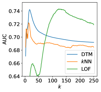
Figure 6: Illustration of parameter $k$’s sensitivity in distance-based methods (DTM, $k$-NN, and LOF). This experiment is conducted on the InternetAds dataset.

Figure 6 indicates that the selection of $k$ significantly impacts the AUC performance for all these three methods, with optimal performance observed only when $k$ is chosen within a relatively small range. Unfortunately, determining the best value for hyper-parameter $k$ is challenging due to the unsupervised nature of the anomaly detection task. Nonetheless, our proposed BRDAD algorithm addresses the aforementioned issue by transforming the anomaly detection problem into a convex optimization problem to determine the weight of each nearest neigbhor.

6 Proofs

In this section, we present proofs of the theoretical results in this paper. More precisely, we first provide proofs related to the surrogate risk in Section 6.1. The proofs related to the convergence rates of BRDDE and BRDAD are provided in Sections 6.2 and 6.3, respectively.

6.1 Proofs Related to the Surrogate Risk

In this section, we first provide proofs related to the error analysis of BWDDE in Section 6.1.1. Then in Section 6.1.2, we present the proof of Proposition 2.3 concerning the surrogate risk.

6.1.1 Proofs Related to Section 4.1

Before we proceed, we present Bernstein’s inequality [8] that will be frequently applied within the subsequent proofs. This concentration inequality is extensively featured in numerous statistical learning compendia, such as [36, 14, 44].

Lemma 1 (Bernstein’s inequality).

Let $B>0$ and $\sigma>0$ be real numbers, and $n\geq 1$ be an integer. Furthermore, let $\xi_{1},\ldots,\xi_{n}$ be independent random variables satisfying $\mathbb{E}_{\mathrm{P}}\xi_{i}=0$, $\|\xi_{i}\|_{\infty}\leq B$, and $\mathbb{E}_{\mathrm{P}}\xi_{i}^{2}\leq\sigma^{2}$ for all $i=1,\ldots,n$. Then for all $\tau>0$, we have

$$\mathrm{P}\biggl{(}\frac{1}{n}\sum_{i=1}^{n}\xi_{i}\geq\sqrt{\frac{2\sigma^{2}\tau}{n}}+\frac{2B\tau}{3n}\biggr{)}\leq e^{-\tau}.$$

To measure the complexity of the functional space, we first recall the definition of the covering number in [49].

Definition 1 (Covering Number).

Let $(\mathcal{X},d)$ be a metric space and $A\subset\mathcal{X}$. For $\varepsilon>0$, the $\varepsilon$-covering number of $A$ is denoted as

$$\mathcal{N}(A,d,\varepsilon):=\min\biggl{\{}n\geq 1:\exists x_{1},\ldots,x_{n}\in\mathcal{X}\text{ such that }A\subset\bigcup^{n}_{i=1}B(x_{i},\varepsilon)\biggr{\}},$$

where $B(x,\varepsilon):=\{x^{\prime}\in\mathcal{X}:d(x,x^{\prime})\leq\varepsilon\}$.

The following Lemma, which is taken from [27] and needed in the proof of Lemma 3, provides the covering number of the indicator functions on the collection of balls in $\mathbb{R}^{d}$.

Lemma 2.

Let $\mathcal{B}:=\{B(x,r):x\in\mathbb{R}^{d},r>0\}$ and $\boldsymbol{1}_{\mathcal{B}}:=\{\boldsymbol{1}_{B}:B\in\mathcal{B}\}$. Then for any $\varepsilon\in(0,1)$, there exists a universal constant $C$ such that

$$\mathcal{N}(\boldsymbol{1}_{\mathcal{B}},\|\cdot\|_{L_{1}(\mathrm{Q})},\varepsilon)\leq C(d+2)(4e)^{d+2}\varepsilon^{-(d+1)}$$

holds for any probability measure $\mathrm{Q}$.

The following lemma, which will be used several times in the sequel, provides the uniform bound on the distance between any point and its $k$-th nearest neighbor with a high probability when the distribution has bounded support.

Lemma 3.

Let Assumption 1 hold. Furthermore, let $\{D_{s}^{b}\}_{b=1}^{B}$ be $B$ disjoint subsets of size $s$ randomly divided from data $D_{n}$ and $R_{s,(i)}^{b}(x)$ be the $i$-distance of $x$ in the subset $D^{b}_{s}$. Moreover, suppose that $s\geq cn^{d/(2+d)}(\log n)^{2/(2+d)}$. Then, there exist some $n_{1}\in\mathbb{N}$ and some constants $0<c_{1}<c_{2}$ such that for all $n>n_{1}$ and $i\geq c_{n}:=\lceil 48(2d+9+8/d)\log n\rceil$, with probability $\mathrm{P}^{n}\otimes\mathrm{P}_{B}$ at least $1-1/(2n^{2})$, there holds

$$c_{1}(i/s)^{1/d}\leq R_{s,(i)}^{b}(x)\leq c_{2}(i/s)^{1/d},\qquad x\in\mathcal{X},\quad b\in[B].$$ (20)

Moreover, we have

$$|\mathrm{P}(B(x,R_{s,(i)}^{b}(x)))-i/s|\lesssim\sqrt{i\log s}/s.$$ (21)

Proof of Lemma 3.

For $x\in\mathcal{X}$ and $q\in[0,1]$, we define the $q$-quantile diameter

$$\rho_{x}(q):=\inf\bigl{\{}r:\mathrm{P}(B(x,r))\geq q\bigr{\}}.$$

Let us first consider the set $\mathcal{B}_{i}^{-}:=\big{\{}B\bigl{(}x,\rho_{x}\bigl{(}(i-\sqrt{3\tau i})/s\bigr{)}\bigr{)}:x\in\mathcal{X}\bigr{\}}\subset\mathcal{B}$. Lemma 2 implies that for any probability $\mathrm{Q}$, there holds

$$\mathcal{N}(\boldsymbol{1}_{\mathcal{B}_{i}^{-}},\|\cdot\|_{L_{1}(\mathrm{Q})},\varepsilon)\leq\mathcal{N}(\boldsymbol{1}_{\mathcal{B}},\|\cdot\|_{L_{1}(\mathrm{Q})},\varepsilon)\leq C(d+2)(4e)^{d+2}\varepsilon^{-(d+1)}.$$ (22)

By the definition of the covering number, there exists an $\varepsilon$-net $\{A_{j}^{-}\}_{j=1}^{J}\subset\mathcal{B}_{k}^{-}$ with $J:=\lfloor C(d+2)(4e)^{d+2}\varepsilon^{-(d+1)}\rfloor$ and for any $x\in\mathcal{X}$, there exists some $j\in\{1,\ldots,J\}$ such that

$$\bigl{\|}\boldsymbol{1}\bigl{\{}B\bigl{(}x,\rho_{x}\bigl{(}(i-\sqrt{3\tau i})/s\bigr{)}\bigr{)}\bigr{\}}-\boldsymbol{1}_{A_{j}^{-}}\bigr{\|}_{L_{1}(D)}\leq\varepsilon.$$ (23)

For any $\ell\in[s]$ and $b\in[B]$, let the random variables $\xi_{\ell,b}$ be defined by $\xi_{\ell,b}=\boldsymbol{1}_{A_{j}^{-}}(X_{\ell}^{b})-(i-\sqrt{3\tau\log s})/s$. Then we have $\mathbb{E}_{\mathrm{P}}\xi_{\ell,b}=0$, $\|\xi_{\ell,b}\|_{\infty}\leq 1$, and $\mathbb{E}_{\mathrm{P}}\xi_{\ell,b}^{2}\leq\mathbb{E}_{\mathrm{P}}\xi_{\ell,b}=(i-\sqrt{3\tau i})/s$. Applying Bernstein’s inequality in Lemma 1, we obtain

$$\frac{1}{s}\sum_{\ell=1}^{s}\boldsymbol{1}_{A_{j}^{-}}(X_{\ell}^{b})-(i-\sqrt{3\tau i})/s\leq\sqrt{2\tau(i-\sqrt{3\tau i})}/s+2\tau/(3s),\qquad b\in[B],$$

with probability $\mathrm{P}^{s}$ at least $1-e^{-\tau}$ . Then the union bound together with the covering number estimation (22) implies that for any $A_{j}^{-}$, $j=1,\cdots,J$, there holds

$$\frac{1}{s}\sum_{\ell=1}^{s}\boldsymbol{1}_{A_{j}^{-}}(X_{\ell}^{b})-(i-\sqrt{3(\tau+\log J)i})/s$$

$$\leq\sqrt{2(\tau+\log J)\bigl{(}i-\sqrt{3(\tau+\log J)i}\bigr{)}}/s+2(\tau+\log J)/(3s).$$

This together with (23) yields that for all $x\in\mathcal{X}$, there holds

$$\frac{1}{s}\sum_{\ell=1}^{s}\boldsymbol{1}\{X_{\ell}\in\rho_{x}\big{(}(i-\sqrt{3\tau i}/s)\big{)}\}-(i-\sqrt{3(\tau+\log J)i})/s$$

$$\leq\sqrt{2(\tau+\log J)\bigl{(}i-\sqrt{3(\tau+\log J)i}\bigr{)}}/s+2(\tau+\log J)/(3s)+\varepsilon.$$

Now, if we take $\varepsilon=1/s$, then for any $s>(4e)\vee(d+2)\vee C$, there holds $\log J=\log C+\log(d+2)+(d+2)\log(4e)+(d+1)\log s\leq(2d+5)\log s$. Let $\tau:=4(2+d)\log s/d+\log(4)$. A simple calculation yields that for all $i\geq c_{n}:=\lceil 48(2d+9+8/d)\log s\rceil$, there holds

$$\sqrt{2(\tau+\log J)\bigl{(}i-\sqrt{3(\tau+\log J)i}\bigr{)}}/s\leq\sqrt{5(\tau+\log J)i/2}/s$$

with probability $\mathrm{P}^{s}$ at least $1-1/(4s^{4(2+d)/d})$. Consequently, for all $n>n_{1}:=\lceil((4e)\vee(d+2)\vee C)^{(2+d)/d}\vee\exp(c^{-(2+d)/2})\rceil$, we have $s>(4e)\vee(d+2)\vee C$ and

$$\sqrt{2(\tau+\log J)\bigl{(}i-\sqrt{3(\tau+\log J)i}\bigr{)}}/s+2(\tau+\log J)/(3s)+1/s\leq\sqrt{3(\tau+\log J)i}/s.$$

with probability $\mathrm{P}^{s}$ at least $1-1/(4n^{4})$. Therefore, for all $x\in\mathcal{X}$, with probability $\mathrm{P}^{s}$ at least $1-1/(4n^{4})$, there holds $\frac{1}{s}\sum_{\ell=1}^{s}\boldsymbol{1}\bigl{\{}B\bigl{(}x,\rho_{x}\bigl{(}(i-\sqrt{3\tau i})/s\bigr{)}\bigr{)}\bigr{\}}(X_{\ell}^{b})\leq i/s$. By the definition of $R_{s,(i)}^{b}(x)$, there holds

$$R_{s,(i)}^{b}(x)\geq\rho_{x}\bigl{(}(i-\sqrt{3\tau i})/s\bigr{)}$$ (24)

with probability $\mathrm{P}^{s}$ at least $1-1/(4n^{4})$. For any $x\in\mathcal{X}$, we have $\mathrm{P}\bigl{(}B\bigl{(}x,\rho_{x}\bigl{(}(i-\sqrt{3\tau i})/s\bigr{)}\bigr{)}\bigr{)}=(i-\sqrt{3\tau i})/s$. By Assumption 1, we have $\mathrm{P}\bigl{(}B\bigl{(}x,\rho_{x}\bigl{(}(i-\sqrt{3\tau i})/s\bigr{)}\bigr{)}\bigr{)}=(i-\sqrt{3\tau i})/s\leq V_{d}\overline{c}\rho_{x}^{d}\bigl{(}(i-\sqrt{3\tau i})/s\bigr{)}\leq(V_{d}\overline{c}/\underline{c})f(x)\rho_{x}^{d}\bigl{(}(i-2\sqrt{3\tau i})/s\bigr{)}$, which yields

$$\rho_{x}\bigl{(}(i-\sqrt{3\tau i})/s\bigr{)}\geq\bigl{(}\underline{c}/(2V_{d}\overline{c})\bigr{)}^{1/d}(i/s)^{1/d}.$$ (25)

Combining (24) with (25), we obtain that $R_{s,(i)}^{b}(x)\gtrsim(i/s)^{1/d}$ holds for all $x\in\mathcal{X}$ with probability $\mathrm{P}^{s}$ at least $1-1/(4n^{4})$. Therefore, a union bound argument yields that for all $n>n_{1}$ and $i\geq c_{n}$, there holds

$$R_{s,(i)}^{b}(x)\geq\rho_{x}\big{(}(i-\sqrt{3\tau i})/s)\bigr{)}\gtrsim(i/s)^{1/d},\qquad x\in\mathcal{X},\quad b\in[B],$$ (26)

with probability $\mathrm{P}^{s}$ at least $1-1/(4n^{3})$. On the other hand, for all $i\geq c_{n}$, there holds

$$R_{s,(i)}^{b}(x)\leq\rho_{x}\bigl{(}(i+\sqrt{3\tau i}/s)\bigr{)}\lesssim(i/s)^{1/d}.$$

Then, applying the union bound argument again, we can show that with probability $\mathrm{P}^{n}\otimes\mathrm{P}_{B}$ at least $1-1/(4n^{2})$, there holds

$$R_{s,(i)}^{b}(x)\lesssim(i/s)^{1/d},\qquad b\in[B].$$ (27)

Combining (26) and (27), we obtain

$$\big{|}\mathrm{P}(B(x,R_{s,(i)}^{b}(x)))-i/s|\leq\big{|} \leq\big{|}\mathrm{P}\big{(}B(x,\rho_{x}((i-\sqrt{3\tau i})/s))\big{)}-i/s\big{|}$$

$$\phantom{=}\vee\big{|}\mathrm{P}\big{(}B(x,\rho_{x}((i+\sqrt{3\tau i})/s))\big{)}-i/s\big{|}\lesssim\sqrt{i\log s}/s$$

with probability $\mathrm{P}^{n}\otimes\mathrm{P}_{B}$ at least $1-1/(2n^{2})$. This completes the proof. ∎

The following lemma, which is needed in the proof of Lemma 5, shows that the $k$-distances are Lipschitz continuous.

Lemma 4.

For $i\in[s]$ and $b\in[B]$, let $R_{s,(i)}^{b}(x)$ be the $i$-distance of $x$ in the subset $D_{s}^{b}=\{X_{1}^{b},\ldots,X_{s}^{b}\}$. Then for any $x$, $x^{\prime}\in\mathcal{X}$, we have $\bigl{|}R_{s,(i)}^{b}(x)-R_{s,(i)}^{b}(x^{\prime})\bigr{|}\leq\|x-x^{\prime}\|_{2}$.

Proof of Lemma 4.

For any fixed $x,x^{\prime}\in\mathcal{X}$, let $g(t):=tx+(1-t)x^{\prime}$ for $t\in[0,1]$ and $\mathrm{L}(x,x^{\prime}):=\{g(t):t\in[0,1]\}$ be the line segment between $x$ and $x^{\prime}$. Let $\Pi([s]\setminus\{\ell\})$ be the collection of the permutations of the set $[s]\setminus\{\ell\}$. For a fixed $i\in[s]$, $\ell\in[s]$, $b\in[B]$, and a permutation $\{\sigma_{m}\}_{m=1}^{s-1}\in\Pi([s]\setminus\{\ell\})$, let $\mathcal{R}_{\ell,\{\sigma_{m}\}_{m=1}^{s-1}}^{b}$ be the subset of $\mathbb{R}^{d}$ satisfying

$$\|x-X_{\sigma_{1}}^{b}\|_{2}\leq\cdots\leq\|x-X_{\sigma_{i-1}}^{b}\|_{2}\leq\|x-X_{\ell}^{b}\|_{2}\leq\|x-X_{\sigma_{i}}^{b}\|_{2}\leq\cdots\leq\|x-X_{\sigma_{s-1}}^{b}\|_{2}.$$ (28)

That is, $X_{\sigma_{1}}^{b},\ldots,X_{\sigma_{i-1}}^{b},X_{\ell}^{b},X_{\sigma_{i}}^{b},\ldots,X_{\sigma_{s-1}}^{b}$ are the nearest neighbors of $x\in\mathcal{R}_{\ell,\{\sigma_{m}\}_{m=1}^{s-1}}^{b}$ in an ascending order. Then we have

$$\mathcal{R}_{\ell,\{\sigma_{m}\}_{m=1}^{s-1}}^{b}= \biggl{(}\bigcap_{j=1}^{i-2}\{x\in\mathbb{R}^{d}:\|x-X_{\sigma_{j}}^{b}\|_{2}\leq\|x-X_{\sigma_{j+1}}^{b}\|_{2}\}\biggr{)}$$

$$\cap\bigl{(}\{x\in\mathbb{R}^{d}:\|x-X_{\sigma_{i-1}}^{b}\|_{2}\leq\|x-X_{\ell}^{b}\|_{2}\}\bigr{)}$$

$$\cap\bigl{(}\{x\in\mathbb{R}^{d}:\|x-X_{\ell}^{b}\|_{2}\leq\|x-X_{\sigma_{i}}^{b}\|_{2}\}\bigr{)}$$

$$\cap\biggl{(}\bigcap_{j=i}^{s-2}\{x\in\mathbb{R}^{d}:\|x-X_{\sigma_{j}}^{b}\|_{2}\leq\|x-X_{\sigma_{j+1}}^{b}\|_{2}\}\biggr{)}.$$

Therefore, $\mathcal{R}_{\ell,\{\sigma_{m}\}_{m=1}^{s-1}}^{b}$ is the intersections of $(s-1)$ half-spaces, which yields that $\mathcal{R}_{\ell,\{\sigma_{m}\}_{m=1}^{s-1}}^{b}$ is a convex subset of $\mathbb{R}^{d}$. Consequently, there exist $0\leq\underline{t}\leq\overline{t}\leq 1$ such that

$$\mathcal{R}_{\ell,\{\sigma_{m}\}_{m=1}^{s-1}}^{b}\cap\mathrm{L}(x,x^{\prime})=g([\underline{t},\overline{t}])\quad\text{ or }\quad\mathcal{R}_{\ell,\{\sigma_{m}\}_{m=1}^{s-1}}^{b}\cap\mathrm{L}(x,x^{\prime})=\emptyset.$$ (29)

Let $\mathcal{R}_{\ell}^{b}$ be the subset of $\mathcal{X}$ whose $i$-th nearest neighbor is $X_{\ell}^{b}$, i.e.,

$$\mathcal{R}_{\ell}^{b}:=\{x\in\mathbb{R}^{d}:X_{\ell}^{b}=X_{(i)}(x;D_{s}^{b})\}.$$

By (28), for every $x\in\mathcal{R}_{\ell}^{b}$, there exists some permutation $\{\sigma_{m}\}_{m=1}^{s-1}\in\Pi([s]\setminus\{\ell\})$ such that $x\in\mathcal{R}_{\ell,\{\sigma_{m}\}_{m=1}^{s-1}}^{b}$. Therefore, we have $\mathcal{R}_{\ell}^{b}\subset\bigcup_{\{\sigma_{m}\}_{m=1}^{s-1}\in\Pi([s]\setminus\{\ell\})}\mathcal{R}_{\ell,\{\sigma_{m}\}_{m=1}^{s-1}}^{b}$. On the other hand, the “$\supset$” relationship holds obviously since for any $\{\sigma_{m}\}_{m=1}^{s-1}\in\Pi([s]\setminus\{\ell\})$ and $x\in\mathcal{R}_{\ell,\{\sigma_{m}\}_{m=1}^{s-1}}^{b}$, we have $x\in\mathcal{R}_{\ell}^{b}$. Therefore, we get

$$\mathcal{R}_{\ell}^{b}=\bigcup_{\{\sigma_{m}\}_{m=1}^{s-1}\in\Pi([s]\setminus\{\ell\})}\mathcal{R}_{\ell,\{\sigma_{m}\}_{m=1}^{s-1}}^{b}.$$

This together with (29) implies that there exist $0\leq t_{1}\leq\cdots\leq t_{J}\leq 1$ such that

$$\mathcal{R}_{\ell}^{b}\cap\mathrm{L}(x,x^{\prime})=\bigcup_{j=1}^{J-1}g([t_{j},t_{j+1}])\quad\text{ or }\quad\mathcal{R}_{\ell}^{b}\cap\mathrm{L}(x,x^{\prime})=\emptyset.$$ (30)

Clearly, we have $\bigcup_{\ell=1}^{s}\bigl{(}\mathcal{R}_{\ell}^{b}\cap\mathrm{L}(x,x^{\prime})\bigr{)}=\mathrm{L}(x,x^{\prime})$. Combining this with (30), we obtain that there exist $t_{1}^{\prime}=0\leq t_{2}^{\prime}\leq\cdots\leq t_{J^{\prime}-1}^{\prime}\leq t^{\prime}_{J^{\prime}}=1$ and $\ell_{1},\ldots,\ell_{J^{\prime}-1}\in[s]$ such that $g([t_{i}^{\prime},t_{i+1}^{\prime}])\subset\mathcal{R}_{\ell_{i}}^{b}$ for all $i\in[J^{\prime}-1]$. Using the triangle inequality, we get

$$|R_{s,(i)}^{b}(g(t_{i}^{\prime}))-R_{s,(i)}^{b}(g(t_{i+1}^{\prime}))|=\bigl{|}\|g(t_{i}^{\prime})-X_{\ell_{i}}^{b}\|_{2}-\|g(t_{i+1}^{\prime})-X_{\ell_{i}}^{b}\|_{2}\bigr{|}\leq\|g(t_{i}^{\prime})-g(t_{i+1}^{\prime})\|_{2}.$$

Therefore, we obtain

$$\bigl{|}R_{s,(i)}^{b}(x) -R_{s,(i)}^{b}(x^{\prime})\bigr{|}=\bigl{|}R_{s,(i)}^{b}(g(t_{1}^{\prime}))-R_{s,(i)}^{b}(g(t_{J^{\prime}}^{\prime}))\bigr{|}$$

$$\leq\sum_{i=1}^{J^{\prime}-1}\bigl{|}R_{s,(i)}^{b}(g(t_{i}^{\prime}))-R_{s,(i)}^{b}(g(t_{i+1}^{\prime}))\bigr{|}\leq\sum_{i=1}^{J^{\prime}-1}\|g(t_{i}^{\prime})-g(t_{i+1}^{\prime})\|_{2}=\|x-x^{\prime}\|_{2}.$$

This completes the proof. ∎

Lemma 5.

Let Assumption 1 hold. Furthermore, let $\{D_{s}^{b}\}_{b=1}^{B}$ be $B$ disjoint subsets of size $s$ randomly divided from data $D_{n}$ with $D_{s}^{b}=\{X_{1}^{b},\ldots,X_{s}^{b}\}$ and $R_{s,(i)}^{b}(x)$ be the $i$-distance of $x$ in the subset $D_{s}^{b}$. Moreover, let $k(w^{b})=\sup\{i\in[s]:w^{b}_{i}\neq 0\}$, $\overline{k}:=\max_{b\in[B]}k(w^{b})$ and suppose that $B\gtrsim\overline{k}\log n$. Finally, let $c_{n}$ be specified as in Lemma 3. Then there exists an $n_{2}\in\mathbb{N}$, which will be specified in the proof, such that for all $x\in\mathcal{X}$ and all $n>n_{2}$, the following statements hold with probability $\mathrm{P}^{n}\otimes\mathrm{P}_{B}$ at least $1-1/n^{2}$:

1. For all $i<c_{n}$, there holds

   $$\frac{1}{B}\sum_{b=1}^{B}w^{b}_{i}\bigl{|}(i/s)^{1/d}-\mathrm{P}(B(x,R_{s,(i)}^{b}(x)))^{1/d}\bigr{|}\lesssim\bigl{(}\overline{k}/s\bigr{)}^{1/d}\sum_{b=1}^{B}w^{b}_{i}/B;$$

2. For all $c_{n}\leq i\leq s$, if $\max_{b\in[B]}w^{b}_{i}\leq V_{i}$, then there holds

   $$\frac{1}{B}\sum_{b=1}^{B}w^{b}_{i}\bigl{|}(i/s)^{1/d}-\mathrm{P}(B(x,R_{s,(i)}^{b}(x)))^{1/d}\bigr{|}\lesssim V_{i}i^{1/d-1/2}s^{-1/d}B^{-1/2}\log^{1/2}n.$$

Proof of Lemma 5.

(i) Let us first consider the case $i\leq c_{n}$. Lemma 3 yields

$$\bigl{|}(i/s)^{1/d}-\mathrm{P}(B(x,R_{s,(i)}^{b}(x)))^{1/d}\bigr{|}\lesssim(c_{n}/s)^{1/d}+\mathrm{P}(B(x,R_{(c_{n})}^{b}(x)))^{1/d}\lesssim(c_{n}/s)^{1/d}\lesssim\bigl{(}\overline{k}/s\bigr{)}^{1/d}.$$

Consequently, we have

$$\frac{1}{B}\sum_{b=1}^{B}w^{b}_{i}\bigl{|}(i/s)^{1/d}-\mathrm{P}(B(x,R_{s,(i)}^{b}(x)))^{1/d}\bigr{|}\lesssim\bigl{(}\overline{k}/s\bigr{)}^{1/d}\sum_{b=1}^{B}w^{b}_{i}/B.$$

(ii) Now, let us consider the case $i>c_{n}$. We first consider the case for a fixed $x\in\mathcal{X}$. Since $\mathrm{P}$ has a density with respect to the Lebesgue measure, the random variable $\|X-x\|_{2}$ is continuous. Therefore, the probability integral transform implies that $\mathrm{P}(B(x,\|X-x\|_{2}))$ follows the uniform distribution over $[0,1]$. For any $b\in[B]$, notice that $X_{1}^{b},\ldots,X_{s}^{b}$ are i.i.d. with the same distribution $\mathrm{P}$. Let $U_{1}^{b},\ldots,U_{s}^{b}$ be i.i.d. uniform $[0,1]$ random variables, then we have

$$\bigl{(}\mathrm{P}(x,\|X_{1}^{b}-x\|_{2}),\ldots,\mathrm{P}(x,\|X_{s}^{b}-x\|_{2})\bigr{)}\overset{\mathcal{D}}{=}\bigl{(}U_{1}^{b},\ldots,U_{s}^{b}\bigr{)}.$$

Using reordered samples with $\|X_{(1)}^{b}(x)-x\|_{2}\leq\cdots\leq\|X_{(s)}^{b}(x)-x\|_{2}$ and the order statistics $U_{(1)}^{b}\leq\cdots\leq U_{(s)}^{b}$, we get

$$\bigl{(}\mathrm{P}(B(x,R_{s,(1)}^{b}(x))),\ldots,\mathrm{P}(B(x,R_{s,(s)}^{b}(x)))\bigr{)}\overset{\mathcal{D}}{=}\big{(}U_{(1)}^{b},\ldots,U_{(s)}^{b}\big{)}.$$ (31)

Therefore, the study of $\mathrm{P}(B(x,R_{s,(i)}^{b}(x)))$ is equivalent to the study of $U_{(i)}$. By Corollary 1.2 in [10], $U_{(i)}^{b}$ is $\mathrm{Beta}(i,s+1-i)$. This implies

$$\mathbb{E}\bigl{(}\mathrm{P}(B(x,R_{s,(i)}^{b}(x)))\bigr{)}=\frac{i}{s+1}\quad\text{and}\quad\mathrm{Var}\bigl{(}\mathrm{P}(B(x,R_{s,(i)}^{b}(x)))\bigr{)}=\frac{i(s-i)}{(s+1)^{2}(s+2)}\leq\frac{i}{s^{2}}.$$

For $i\geq c_{n}\gtrsim\log s$, (21) yields that for all $n\geq n_{1}$ with $n_{1}$ specified as in Lemma 3, there holds

$$\bigl{|}i/(s+1)-\mathrm{P}(B(x,R_{s,(i)}^{b}(x)))\bigr{|}\lesssim i/(s+1)+\sqrt{i\log s}/s\lesssim i/s$$

with probability $\mathrm{P}^{n}\otimes\mathrm{P}_{B}$ at least $1-1/(2n^{2})$. For a fixed $i\geq c_{n}$, since $\mathrm{P}(B(x,R_{s,(i)}^{b}(x)))$, $b\in[B]$ are i.i.d. random variables, by applying Bernstein’s inequality in Lemma 1, we obtain

$$\frac{1}{B}\sum_{b=1}^{B}\bigl{|}i/(s+1)-\mathrm{P}(B(x,R_{s,(i)}^{b}(x)))\bigr{|}\lesssim\sqrt{\frac{i\log n}{Bs^{2}}}+\frac{i\log n}{Bs}$$

with probability $\mathrm{P}^{n}\otimes\mathrm{P}_{B}$ at least $1-1/(4n^{2d+4})$. This together with (31) yields

$$\frac{1}{B}\sum_{b=1}^{B}\bigl{|}i/s-\mathrm{P}(B(x,R_{s,(i)}^{b}(x)))\bigr{|}\lesssim\sqrt{\frac{i\log n}{Bs^{2}}}+\frac{i\log n}{Bs}+\frac{1}{s(s+1)}.$$

Then, using the condition $B\gtrsim\overline{k}\log n$ and the union-bound argument, we obtain that for all $c_{n}\leq i\leq s$, there holds

$$\frac{1}{B}\sum_{b=1}^{B}\bigl{|}i/s-\mathrm{P}(B(x,R_{s,(i)}^{b}(x)))\bigr{|}\lesssim\sqrt{\frac{i\log n}{Bs^{2}}}$$ (32)

with probability $\mathrm{P}^{n}\otimes\mathrm{P}_{B}$ at least $1-1/(4n^{2d+3})$. By Lemma 3, for all $i\geq c_{n}$, we have $R_{s,(i)}^{b}(x)\gtrsim(i/s)^{1/d}$. This together with $\|f\|_{\infty}\geq\underline{c}$ in Assumption 1 implies that $\mathrm{P}(B(x,R_{s,(i)}^{b}(x)))\gtrsim R_{s,(i)}^{b}(x)^{d}\gtrsim i/s$. Therefore, we have

$$\sum_{j=1}^{d}(i/s)^{j/d}\mathrm{P}(B(x,R_{s,(i)}^{b}(x)))^{(d-1-j)/d}\gtrsim\sum_{j=1}^{d}(i/s)^{(d-1)/d}\gtrsim(i/s)^{(d-1)/d}.$$

Combining this with (15) and (32), we obtain

$$\frac{1}{B}\sum_{b=1}^{B}\bigl{|}(i/s)^{1/d}-\mathrm{P}(B(x,R_{s,(i)}^{b}(x)))^{1/d}\bigr{|}\lesssim i^{1/d-1/2}s^{-1/d}B^{-1/2}\log^{1/2}n.$$

This together with the condition $\max_{b\in[B]}w^{b,*}\leq V_{i}$ implies that for any fixed $x\in\mathcal{X}$ and all $i>c_{n}$, there holds

$$\frac{1}{B}\sum_{b=1}^{B}w^{b,*}_{i}\bigl{|}(i/s)^{1/d}-\mathrm{P}(B(x,R_{s,(i)}^{b}(x)))^{1/d}\bigr{|}\lesssim V_{i}i^{1/d-1/2}s^{-1/d}B^{-1/2}\sqrt{\log n}.$$

Since $\mathcal{X}=[0,1]^{d}$ is the rectangle in the Euclidean space $\mathbb{R}^{d}$, we can choose an $n^{-1/d-1}$-net $\{z_{j}\}_{j=1}^{J}$ of $\mathcal{X}$ such that $J\leq(d^{1/2}n^{1/d+1})^{d}=d^{d/2}n^{d+1}$. Using the union-bound argument, we obtain that for all $j\in[J]$ and $i>c_{n}$ with $n>n_{2}:=\max\{n_{1},d\}$, there holds

$$\frac{1}{B}\sum_{b=1}^{B}w^{b,*}_{i}\bigl{|}(i/s)^{1/d}-\mathrm{P}(B(z_{j},R_{s,(i)}^{b}(z_{j})))^{1/d}\bigr{|}\lesssim V_{i}i^{1/d-1/2}s^{-1/d}B^{-1/2}\sqrt{\log n}$$ (33)

with probability $\mathrm{P}_{n}\otimes\mathrm{P}_{B}$ at least $1-d^{d/2}n^{d+1}/(4n^{2d+3})\geq 1-1/(4n^{2})$. Since $\{z_{j}\}_{j=1}^{J}$ is an $n^{-1/d-1}$-net of $\mathcal{X}$, for any $x\in\mathcal{X}$, there exists a $z_{j}$ such that $\|x-z_{j}\|_{2}\leq n^{-1/d-1}$. Using the triangle inequality, we get

$$\frac{1}{B}\sum_{b=1}^{B}w^{b,*}_{i}\bigl{|}(i/s)^{1/d}-\mathrm{P}(B(x,R_{s,(i)}^{b}(x)))^{1/d}\bigr{|}$$

$$\leq\frac{1}{B}\sum_{b=1}^{B}w^{b,*}_{i}\bigl{|}\mathrm{P}(B(x,R_{s,(i)}^{b}(x)))^{1/d}-\mathrm{P}(B(z_{j},R_{s,(i)}^{b}(z_{j})))^{1/d}\bigr{|}$$

$$\phantom{=}+\frac{1}{B}\sum_{b=1}^{B}w^{b,*}_{i}\bigl{|}(i/s)^{1/d}-\mathrm{P}(B(z_{j},R_{s,(i)}^{b}(z_{j})))^{1/d}\bigr{|}$$

$$\lesssim\frac{1}{B}\sum_{b=1}^{B}w^{b,*}_{i}\bigl{|}\mathrm{P}(B(x,R_{s,(i)}^{b}(x)))^{1/d}-\mathrm{P}(B(z_{j},R_{s,(i)}^{b}(z_{j})))^{1/d}\bigr{|}$$

$$\phantom{=}+V_{i}i^{1/d-1/2}s^{-1/d}B^{-1/2}\sqrt{\log n}.$$ (34)

By (15), we have

$$\bigl{|}\mathrm{P}(B(x,R_{s,(i)}^{b}(x)))^{1/d}-\mathrm{P}(B(z_{j},R_{s,(i)}^{b}(z_{j})))^{1/d}\bigr{|}$$

$$\lesssim\frac{\bigl{|}\mathrm{P}(B(x,R_{s,(i)}^{b}(x)))-\mathrm{P}(B(z_{j},R_{s,(i)}^{b}(z_{j})))\bigr{|}}{\sum_{j=0}^{d-1}\mathrm{P}(B(x,R_{s,(i)}^{b}(x)))^{j/d}\mathrm{P}(B(z_{j},R_{s,(i)}^{b}(z_{j})))^{(d-1-j)/d}}$$

$$\lesssim(i/s)^{-(d-1)/d}\bigl{|}\mathrm{P}(B(x,R_{s,(i)}^{b}(x)))-\mathrm{P}(B(z_{j},R_{s,(i)}^{b}(z_{j})))\bigr{|},$$ (35)

where the last inequality follows from Lemma 3 and the condition $i>c_{n}$. Using the triangle inequality again, we get

$$\bigl{|}\mathrm{P}(B(x,R_{s,(i)}^{b}(x)))-\mathrm{P}(B(z_{j},R_{s,(i)}^{b}(z_{j})))\bigr{|}$$

$$\leq\bigl{|}\mathrm{P}(B(x,R_{s,(i)}^{b}(x)))-\mathrm{P}(B(z_{j},R_{s,(i)}^{b}(x)))\bigr{|}$$

$$\phantom{=}+\bigl{|}\mathrm{P}(B(z_{j},R_{s,(i)}^{b}(x)))-\mathrm{P}(B(z_{j},R_{s,(i)}^{b}(z_{j})))\bigr{|}.$$ (36)

For the first term on the right-hand side of (6.1.1), the Lipschitz continuity of the density function $f$ in Assumption 1 yields

$$\bigl{|}\mathrm{P}(B(x,R_{s,(i)}^{b}(x)))-\mathrm{P}(B(z_{j},R_{s,(i)}^{b}(x)))\bigr{|}$$

$$=\biggl{|}\int_{B(x,R_{s,(i)}^{b}(x))}f(y)\,dy-\int_{B(z_{j},R_{s,(i)}^{b}(x))}f(y)\,dy\biggr{|}$$

$$=\biggl{|}\int_{B(x,R_{s,(i)}^{b}(x))}f(y)\,dy-\int_{B(x,R_{s,(i)}^{b}(x))}f(y+z_{j}-x)\,dy\biggr{|}$$

$$\lesssim\int_{B(x,R_{s,(i)}^{b}(x))}\bigl{|}f(y)-f(y+z_{j}-x)\bigr{|}\,dy\leq c_{L}\int_{B(x,R_{s,(i)}^{b}(x))}\|z_{j}-x\|_{2}\,dy$$

$$\leq c_{L}R_{s,(i)}^{b}(x)^{d}\|z_{j}-x\|_{2}\lesssim(i/s)\|z_{j}-x\|_{2}\lesssim(i/s)n^{-1/d-1}.$$ (37)

Let us consider the second term on the right-hand side of (6.1.1). By the condition $\|f\|_{\infty}\leq\overline{c}$ in Assumption 1, we have

$$\bigl{|}\mathrm{P}(B(z_{j},R_{s,(i)}^{b}(x)))-\mathrm{P}(B(z_{j},R_{s,(i)}^{b}(z_{j})))\bigr{|}\leq\bigl{|}\mu(B(z_{j},R_{s,(i)}^{b}(x)))-\mu(B(z_{j},R_{s,(i)}^{b}(z_{j})))\bigr{|}.$$

Lemma 4 together with the inequality $\|z_{j}-x\|_{2}\leq n^{-1/d-1}$ implies

$$\bigl{|}R_{s,(i)}^{b}(x))-R_{s,(i)}^{b}(z_{j}))\bigr{|}\leq\|x-z_{j}\|_{2}\leq c_{1}(c_{n}/n)^{1/d}\leq c_{1}(c_{n}/s)^{1/d}\lesssim(R_{s,(i)}^{b}(x)\wedge R_{s,(i)}^{b}(z_{j})),$$

which yields

$$\bigl{|}\mu(B(z_{j},R_{s,(i)}^{b}(x)))-\mu(B(z_{j},R_{s,(i)}^{b}(z_{j})))\bigr{|} \lesssim\bigl{(}(R_{s,(i)}^{b}(x)\vee R_{s,(i)}^{b}(z_{j}))\bigr{)}^{d-1}\|x-z_{j}\|_{2}$$

$$\lesssim(i/s)^{(d-1)/d}\|x-z_{j}\|_{2}.$$

Consequently we have

$$\bigl{|}\mathrm{P}(B(z_{j},R_{s,(i)}^{b}(x)))-\mathrm{P}(B(z_{j},R_{s,(i)}^{b}(z_{j})))\bigr{|}\lesssim(i/s)^{(d-1)/d}\|x-z_{j}\|_{2}.$$

Combining this with (6.1.1) and (6.1.1), we get

$$\bigl{|}\mathrm{P}(B(x,R_{s,(i)}^{b}(x)))-\mathrm{P}(B(z_{j},R_{s,(i)}^{b}(z_{j})))\bigr{|}\lesssim(i/s)^{(d-1)/d}\|x-z_{j}\|_{2}.$$

This together with (45) yields

$$\bigl{|}\mathrm{P}(B(x,R_{s,(i)}^{b}(x)))^{1/d}-\mathrm{P}(B(z_{j},R_{s,(i)}^{b}(z_{j})))^{1/d}\bigr{|}\lesssim\|z_{j}-x\|_{2}\lesssim i^{1/d-1/2}s^{-1/d}B^{-1/2}\sqrt{\log n},$$

Consequently we obtain

$$\frac{1}{B}\sum_{b=1}^{B}w^{b,*}_{i}\bigl{|}\mathrm{P}(B(x,R_{s,(i)}^{b}(x)))^{1/d}-\mathrm{P}(B(z_{j},R_{s,(i)}^{b}(z_{j})))^{1/d}\bigr{|}\lesssim V_{i}i^{1/d-1/2}s^{-1/d}B^{-1/2}\sqrt{\log n}.$$

This together with (6.1.1) yields

$$\frac{1}{B}\sum_{b=1}^{B}w^{b,*}_{i}\bigl{|}(i/s)^{1/d}-\mathrm{P}(B(z_{j},R_{s,(i)}^{b}(z_{j})))^{1/d}\bigr{|}\lesssim V_{i}i^{1/d-1/2}s^{-1/d}B^{-1/2}\sqrt{\log n}$$

for any $x\in\mathcal{X}$. This completes the proof. ∎

Proof of Proposition 2.

Proof of Bounding $(I)$. Let $(IV)$ and $(V)$ be defined by

$$(IV):=\sum_{j=0}^{d-1}\biggl{(}\frac{1}{B}\sum_{b=1}^{B}\sum_{i=1}^{s}w_{i}^{b}(i/s)^{1/d}\biggr{)}^{j}\bigl{(}f(x)V_{d}R_{n}^{B}(x)\bigr{)}^{(d-1-j)/d}\,\text{ and }\,(V):=V_{d}R_{n}^{B}(x)^{d}.$$

Then by (14) and (15), in order to derive the upper bound of $(I)$, it suffices to derive the upper bound of $(IV)$ and the lower bound of $(V)$.

Let us first consider $(IV)$. By Condition (ii), we have

$$\sum_{i=1}^{s}w_{i}^{b}(i/s)^{1/d}\asymp\bigl{(}k^{b}/s\bigr{)}^{1/d}\lesssim\bigl{(}\overline{k}/s\bigr{)}^{1/d}.$$ (38)

Consequently we get

$$\biggl{(}\frac{1}{B}\sum_{b=1}^{B}\sum_{i=1}^{s}w_{i}^{b}(i/s)^{1/d}\biggr{)}^{j}\lesssim\bigl{(}\overline{k}/s\bigr{)}^{j/d}.$$

On the other hand, Lemma 3 yields

$$R_{s}^{w,b}(x) =\sum_{i=1}^{s}w_{i}^{b}R_{s,(i)}^{b}(x)=\sum_{i=1}^{c_{n}}w_{i}^{b}R_{s,(i)}^{b}(x)+\sum_{i=c_{n}+1}^{n}w_{i}^{b}R_{s,(i)}^{b}(x)$$

$$\leq R_{s,(c_{n})}^{b}(x)+\sum_{i=c_{n}+1}^{n}w_{i}^{b}R_{s,(i)}^{b}(x)\lesssim(k^{b}/s)^{1/d}+\sum_{i=1}^{k^{b}}w_{i}^{b}(i/s)^{1/d}\lesssim\bigl{(}\overline{k}/s\bigr{)}^{1/d}.$$

Consequently we obtain

$$R_{n}^{B}(x)=\frac{1}{B}\sum_{b=1}^{B}R_{s}^{w,b}(x)\lesssim\bigl{(}\overline{k}/s\bigr{)}^{1/d}.$$ (39)

This together with (38) and $\|f\|_{\infty}\leq\overline{c}$ in Assumption 1 yields

$$(IV)\lesssim\sum_{j=0}^{d-1}\bigl{(}\overline{k}/s\bigr{)}^{j/d}\cdot f(x)^{(d-1-j)/d}\cdot\bigl{(}\overline{k}/s\bigr{)}^{(d-1-j)/d}\lesssim\bigl{(}\overline{k}/s\bigr{)}^{(d-1)/d}.$$ (40)

Next, let us consider $(V)$. By Lemma 3, for all $n>n_{1}$, there holds

$$R_{s}^{w,b}(x)\gtrsim\sum_{i=c_{n}+1}^{n}w_{i}^{b}R_{s,(i)}^{b}(x) \gtrsim\sum_{i=1}^{s}w_{i}^{b}(i/s)^{1/d}=\sum_{i=1}^{s}w_{i}^{b}(i/s)^{1/d}-\sum_{i=1}^{c_{n}}w_{i}^{b}(i/s)^{1/d}$$

$$\gtrsim\bigl{(}k^{b}/s\bigr{)}^{1/d}-(c_{n}/s)^{1/d}\gtrsim\bigl{(}k^{b}/s\bigr{)}^{1/d}\gtrsim\bigl{(}\underline{k}/s\bigr{)}^{1/d},$$ (41)

which implies

$$R_{n}^{B}(x)=\frac{1}{B}\sum_{b=1}^{B}R_{s}^{w,b}(x)\gtrsim(\underline{k}/s)^{1/d}.$$ (42)

Thus we get $(V)=V_{d}R_{n}^{B}(x)^{d}\gtrsim\underline{k}/s$. This together with (40) and $\overline{k}\asymp\underline{k}$ in Condition (iii) implies $(I)=(IV)/(V)\lesssim\bigl{(}\overline{k}/s\bigr{)}^{-1/d}$, which completes the proof of bounding $(I)$.

Proof of Bounding $(II)$. Lemma 5 (i) yields that for all $x\in\mathcal{X}$, there holds

$$\frac{1}{B}\sum_{b=1}^{B}w^{b}_{i}\bigl{|}(i/s)^{1/d}-\mathrm{P}(B(x,R_{s,(i)}^{b}(x)))^{1/d}\bigr{|}\lesssim\bigl{(}\overline{k}/s\bigr{)}^{1/d}\cdot\frac{1}{B}\sum_{b=1}^{B}w^{b}_{i}.$$

Using $\sum_{i=1}^{c_{n}}w_{i}^{b}\lesssim\log n/k^{b}$ in Condition (i), we get

$$\sum_{i=1}^{c_{n}}\frac{1}{B}\sum_{b=1}^{B}w^{b}_{i}\bigl{|}(i/s)^{1/d}-\mathrm{P}(B(x,R_{s,(i)}^{b}(x)))^{1/d}\bigr{|}\lesssim(\log n/\underline{k})\cdot(\overline{k}/s)^{1/d}.$$ (43)

On the other hand, Lemma 5 implies

$$\sum_{i=c_{n}+1}^{s}\frac{1}{B}\sum_{b=1}^{B}w^{b}_{i}\bigl{|}(i/s)^{1/d}-\mathrm{P}(B(x,R_{s,(i)}^{b}(x)))^{1/d}\bigr{|} \lesssim\sum_{i=c_{n}+1}^{s}V_{i}i^{1/d-1/2}s^{-1/d}B^{-1/2}\log^{1/2}n.$$

for all $n>n_{2}$. Using $\sum_{i=c_{n}}^{s}V_{i}i^{1/d-1/2}\lesssim\bigl{(}\overline{k}\bigr{)}^{1/d-1/2}$ in Condition (i), we obtain

$$\sum_{i=c_{n}+1}^{s}\frac{1}{B}\sum_{b=1}^{B}w^{b}_{i}\bigl{|}(i/s)^{1/d}-\mathrm{P}(B(x,R_{s,(i)}^{b}(x)))^{1/d}\bigr{|} \lesssim\bigl{(}\overline{k}/s\bigr{)}^{1/d}\bigl{(}\log n/(\overline{k}B)\bigr{)}^{1/2}.$$

This together with (43) and $\log s\gtrsim\log n$ implies

$$(II)\lesssim(\log s/\underline{k})\cdot(\overline{k}/s)^{1/d}+\bigl{(}\overline{k}/s\bigr{)}^{1/d}\bigl{(}\log s/(\overline{k}B)\bigr{)}^{1/2},$$

which completes the proof of bounding $(II)$.

Proof of Bounding $(III)$. Using (15) and $\|f\|_{\infty}\geq\underline{c}$ in Assumption 1, we get

$$\bigl{|}(\mathrm{P}(B(x,R_{s,(i)}^{b}(x))))^{1/d}-V_{d}^{1/d}f(x)^{1/d}R_{s,(i)}^{b}(x)\bigr{|}\lesssim\frac{\bigl{|}\mathrm{P}(B(x,R_{s,(i)}^{b}(x)))-V_{d}f(x)R_{s,(i)}^{b}(x)^{d}\bigr{|}}{\sum_{j=0}^{d-1}\mathrm{P}(B(x,R_{s,(i)}^{b}(x)))^{j/d}R_{s,(i)}^{b}(x)^{d-1-j}}.$$

The Lipschitz smoothness in Assumption 1 and the condition $B(x,R_{s,(k^{b})}^{b}(x))\subset[0,1]^{d}$ yield

$$\bigl{|}\mathrm{P}(B(x,R_{s,(i)}^{b}(x)))-V_{d}f(x)R_{s,(i)}^{b}(x)^{d}\bigr{|}$$

$$=\biggl{|}\int_{B(x,R_{s,(i)}^{b}(x))}f(y)\,dy-\int_{B(x,R_{s,(i)}^{b}(x)}f(x)\,dy\biggr{|}\leq\int_{B(x,R_{s,(i)}^{b}(x))}|f(y)-f(x)|\,dy$$

$$\leq c_{L}\int_{B(x,R_{s,(i)}^{b}(x))}\|y-x\|_{2}\,dy\lesssim R_{s,(i)}^{b}(x)^{d+1}\lesssim(i/s)R_{s,(i)}^{b}(x).$$ (44)

On the other hand, $\|f\|_{\infty}\geq\underline{c}$ in Assumption 1 together with $R_{s,(i)}^{b}(x)\asymp(i/s)^{1/d}$ in Lemma 3 yields that $\mathrm{P}(B(x,R_{s,(i)}^{b}(x)))\gtrsim i/s$ holds for $i\geq c_{n}$. Consequently we obtain

$$\sum_{j=0}^{d-1}(i/s)^{j/d}\bigl{(}R_{s,(i)}^{b}(x)\bigr{)}^{(d-1-j)/d}\gtrsim\sum_{j=0}^{d-1}(i/s)^{j/d}\cdot(i/s)^{(d-1-j)/d}\gtrsim(i/s)^{(d-1)/d},\qquad i\geq c_{n}+1.$$

This together with (6.1.1) implies

$$\bigl{|}(\mathrm{P}(B(x,R_{s,(i)}^{b}(x))))^{1/d}-V_{d}^{1/d}f(x)^{1/d}R_{s,(i)}^{b}(x)\bigr{|}\lesssim(i/s)^{1/d}R_{s,(i)}^{b}(x),\qquad i\geq c_{n}+1.$$ (45)

Therefore, we have

$$\sum_{i=c_{n}+1}^{k^{b}}w_{i}^{b}\bigl{|}(\mathrm{P}(B(x,R_{s,(i)}^{b}(x))))^{1/d}-V_{d}^{1/d}f(x)^{1/d}R_{s,(i)}^{b}(x)\bigr{|}\lesssim(\overline{k}/s)^{1/d}\sum_{i=1}^{s}w_{i}^{b}R_{s,(i)}^{b}(x).$$

Lemma 3 together with the condition $\sum_{i=1}^{s}w_{i}^{b}i^{1/d}\asymp\bigl{(}k^{b}\bigr{)}^{1/d}$ yields that $w_{i}^{b}R_{s,(i)}^{b}(x)\lesssim w_{i}^{b}(i/s)^{1/d}\lesssim(k^{b}/s)^{1/d}$. Consequently we have

$$\frac{1}{B}\sum_{b=1}^{B}\sum_{i=c_{n}+1}^{k^{b}}w_{i}^{b}\bigl{|}(\mathrm{P}(B(x,R_{s,(i)}^{b}(x))))^{1/d}-V_{d}^{1/d}f(x)^{1/d}R_{s,(i)}^{b}(x)\bigr{|}\lesssim(\overline{k}/s)^{1/d}.$$ (46)

On the other hand, Lemma 3 yields that for $1\leq i\leq c_{n}$, there holds

$$\sum_{i=1}^{c_{n}}w_{i}^{b}\bigl{|}\mathrm{P}(B(x,R_{s,(i)}^{b}(x)))^{1/d}-V_{d}^{1/d}f(x)^{1/d}R_{s,(i)}^{b}(x)\bigr{|}\lesssim(c_{n}/s)^{1/d}\sum_{i=1}^{c_{n}}w_{i}^{b}\lesssim\bigl{(}\overline{k}/s\bigr{)}^{1/d}\sum_{i=1}^{c_{n}}w_{i}^{b}.$$

This together with $\sum_{i=1}^{c_{n}}w_{i}^{b}\lesssim\log s/k^{b}$ in Condition (i) implies

$$\sum_{i=1}^{c_{n}}w_{i}^{b}\bigl{|}\mathrm{P}(B(x,R_{s,(i)}^{b}(x)))^{1/d}-V_{d}^{1/d}f(x)^{1/d}R_{s,(i)}^{b}(x)\bigr{|}\lesssim\bigl{(}\overline{k}/s\bigr{)}^{1/d}\bigl{(}\log s/\overline{k}\bigr{)}.$$

Therefore, we obtain

$$\frac{1}{B}\sum_{b=1}^{B}\sum_{i=1}^{c_{n}}w_{i}^{b}\bigl{|}\mathrm{P}(B(x,R_{s,(i)}^{b}(x)))^{1/d}-V_{d}^{1/d}f(x)^{1/d}R_{s,(i)}^{b}(x)\bigr{|}\lesssim\bigl{(}\overline{k}/s\bigr{)}^{1/d}\bigl{(}\log s/\overline{k}\bigr{)}.$$

Combining this with (46), we obtain $(III)\lesssim\bigl{(}\overline{k}/s\bigr{)}^{1/d}\bigl{(}\log s/\overline{k}\bigr{)}+\bigl{(}\overline{k}/s\bigr{)}^{2/d}$, which completes the proof of bounding $(III)$. Therefore, we show that for all $n>N_{1}:=n_{!}\wedge n_{2}$, all the statements holds with probability $\mathrm{P}_{n}\otimes\mathrm{P}_{B}$ at least $1-1/n^{2}$. ∎

6.1.2 Proofs Related to Section 2.3

To prove Proposition 1, we need the following lemma, which provides the upper bound of the numbers of the instances near the boundary.

Lemma 6.

Let the dataset $D_{n}$ be randomly and evenly divided into $B$ disjoint subsets $\{D_{s}^{b}\}_{b=1}^{B}$ with $D_{s}^{b}=\{X_{1}^{b},\ldots,X_{s}^{b}\}$. Moreover, let $\Delta_{n}:=[-1+c_{2}(\overline{k}/s)^{1/d},1-c_{2}(\overline{k}/s)^{1/d}]$ with the constant $c_{2}$ specified as in Lemma 3, $\mathcal{I}_{s}^{b}:=\{i\in[s]:X_{i}^{b}\in\Delta_{n}\}$, and $n_{s}^{b}:=|\mathcal{I}_{s}^{b}|$. Then for all $b\in[B]$, there holds $1-n_{s}^{b}/s\lesssim\bigl{(}k^{b}/s\bigr{)}^{1/d}$ with probability $\mathrm{P}_{n}\otimes\mathrm{P}_{B}$ at least $1-1/n^{2}$.

Proof of Lemma 6.

Let $\Delta_{n}^{c}:=[0,1]^{d}\setminus\Delta_{n}$. For $\ell\in[s]$ and $b\in[B]$, we define $\xi_{\ell,b}^{\prime}:=\boldsymbol{1}_{\Delta_{n}^{c}}(X_{\ell}^{b})-\mathrm{P}(x:x\in\Delta_{n}^{c})$. Then we have $\mathbb{E}_{\mathrm{P}}\xi_{\ell,b}^{\prime}=0$and $\mathbb{E}_{\mathrm{P}}(\xi_{\ell,b}^{\prime})^{2}\leq\mathbb{E}_{\mathrm{P}}\xi_{\ell,b}^{\prime}\leq\mu(\Delta_{n}^{c})\lesssim\bigl{(}k^{b}/s\bigr{)}^{1/d}$. Applying Bernstein’s inequality in Lemma 1, we obtain

$$\frac{1}{s}\sum_{\ell=1}^{s}\boldsymbol{1}_{\Delta_{n}^{c}}(X_{\ell}^{b})-\mathrm{P}(\Delta_{n}^{c})\lesssim\sqrt{2(k^{b}/s)^{1/d}\tau/n}+2\tau/(3n)$$

with probability $\mathrm{P}^{s}$ at least $1-e^{-\tau}$. With $\tau:=3\log n+\log 4$ we obtain

$$1-n_{s}^{b}/s=\frac{1}{s}\sum_{\ell=1}^{s}\boldsymbol{1}_{\Delta_{n}^{c}}(X_{\ell}^{b})\lesssim\bigl{(}k^{b}/s\bigr{)}^{1/d}+\sqrt{(k^{b}/s)^{1/d}\tau/n}+\log n/n\lesssim\bigl{(}k^{b}/s\bigr{)}^{1/d}$$

with probability $\mathrm{P}^{s}$ at least $1-1/(4n^{3})$. Then, by the union bound argument, the above inequality holds for all $b\in[B]$ with probability $\mathrm{P}^{n}\otimes\mathrm{P}_{B}$ at least $1-1/(4n^{2})$. This completes the proof. ∎

Proof of Proposition 1.

Proposition 2 together with (19) implies that for all $n>N_{1}^{*}:=N_{1}$ and $X_{i}^{b}$ satisfying $B(X_{i}^{b},R_{s,(k^{b})}^{b}(X_{i}^{b}))\subset[0,1]^{d}$, $b\in[B]$, there holds

$$L(X_{i}^{b},f_{n}^{B})=\bigl{|}f_{n}^{B}(X_{i}^{b})-f(X_{i}^{b})\bigr{|}\lesssim\log s/\underline{k}+\bigl{(}\log s/(\overline{k}B)\bigr{)}^{1/2}+(\overline{k}/s)^{1/d}$$

with probability $\mathrm{P}^{n}\otimes\mathrm{P}_{B}$ at least $1-3/(4n^{2})$. The conditions $\|w^{b}\|_{2}\gtrsim\bigl{(}k^{b}\bigr{)}^{-1/2}$ and $\underline{k}\asymp\overline{k}$ yield that $\frac{1}{B}\sum_{b=1}^{B}\|w^{b}\|_{2}\gtrsim\frac{1}{B}\sum_{b=1}^{B}\bigl{(}k^{b}\bigr{)}^{-1/2}\gtrsim(\underline{k})^{-1/2}\gtrsim(\overline{k})^{-1/2}$. Therefore, we obtain

$$\bigl{(}\log s/(\overline{k}B)\bigr{)}^{1/2}\lesssim\frac{1}{B}\sum_{b=1}^{B}\sqrt{\log s/B}\cdot\|w^{b}\|_{2}.$$ (47)

Notice that (6.1.1) implies

$$R_{s}^{w,b}(X_{i}^{b})\gtrsim\bigl{(}\underline{k}/s\bigr{)}^{1/d}.$$ (48)

On the other hand, the condition $B\asymp\overline{k}\log n$ implies that $\log s/\underline{k}\lesssim(\log s)^{2}/B$. Combining this with (47) and (48), we obtain

$$\bigl{|}f_{n}^{B}(X_{i}^{b})-f(X_{i}^{b})\bigr{|}\lesssim\sqrt{\log s/B}\cdot\|w^{b}\|_{2}+R^{w,b}_{s}(X_{i}^{b})+(\log s)^{2}/B.$$

This completes the proof of (3).

Next, let us turn to the proof of (1). Let $\Delta_{n}=[-1+c_{2}(\overline{k}/s)^{1/d},1-c_{2}(\overline{k}/s)^{1/d}]$ with the constant $c_{2}$ specified as in Lemma 3, $\mathcal{I}_{s}^{b}=\{i\in[s]:X_{i}^{b}\in\Delta_{n}\}$, and $n_{s}^{b}=|\mathcal{I}_{s}^{b}|$. Then, it is clear to see that

$$\mathcal{R}_{L,\mathrm{D}_{n}}(f_{n}^{B}) =\frac{1}{B}\sum_{b=1}^{B}\frac{1}{s}\sum_{i=1}^{s}\bigl{|}f_{n}^{B}(X_{i}^{b})-f(X_{i}^{b})\bigr{|}$$

$$=\frac{1}{B}\sum_{b=1}^{B}\frac{1}{s}\biggl{(}\sum_{i\in\mathcal{I}_{s}^{b}}\bigl{|}f_{n}^{B}(X_{i}^{b})-f(X_{i}^{b})\bigr{|}+\sum_{i\in[s]\setminus\mathcal{I}_{s}^{b}}\bigl{|}f_{n}^{B}(X_{i}^{b})-f(X_{i}^{b})\bigr{|}\biggr{)}.$$ (49)

Let us consider the first term on the right-hand side of (6.1.2). For any $x\in\Delta_{n}$ and $y\in B(x,R_{s,(k^{b})}^{b}(x))$ for $b\in[B]$, we have $d(y,\mathbb{R}^{d}\setminus[0,1]^{d})\geq c_{2}(\overline{k}/s)^{1/d}-R_{s,(k^{b})}^{b}(x)\geq 0$, where the last inequality follows from Lemma 3. This implies that $B(x,R_{s,(k^{b})}^{b}(x))\subset[0,1]^{d}$ for any $x\in\Delta_{n}$ and $b\in[B]$. Therefore, by (3), we have

$$\sum_{i\in\mathcal{I}_{s}^{b}}\bigl{|}f_{n}^{B}(X_{i}^{b})-f(X_{i}^{b})\bigr{|}\lesssim\sum_{i=1}^{s}\biggl{(}\sqrt{\log s/B}\cdot\|w^{b}\|_{2}+R^{w,b}_{s}(X_{i}^{b})+(\log s)^{2}/B\biggr{)},$$

which implies

$$\frac{1}{B}\sum_{b=1}^{B}\frac{1}{s}\sum_{i\in\mathcal{I}_{s}^{b}}\bigl{|}f_{n}^{B}(X_{i}^{b})-f(X_{i}^{b})\bigr{|}\lesssim\frac{1}{B}\sum_{b=1}^{B}\biggl{(}\sqrt{\frac{\log s}{B}}\cdot\|w^{b}\|_{2}+\frac{1}{s}\sum_{i=1}^{s}R^{w,b}_{s}(X_{i}^{b})+\frac{(\log s)^{2}}{B}\biggr{)}.$$ (50)

On the other hand, let us consider the second term on the right-hand side of (6.1.2). The condition $\sum_{i=1}^{s}i^{1/d}w_{i}^{b}\asymp\bigl{(}k^{b}\bigr{)}^{1/d}$, $b\in[B]$, together with (42) in the proof of Proposition 2 implies that for all $x\in[0,1]^{d}$, there holds

$$f_{n}^{B}(x)=\frac{1}{V_{d}R_{n}^{B}(x)^{d}}\biggl{(}\frac{1}{B}\sum_{b=1}^{B}\sum_{i=1}^{s}w_{i}^{b}(i/s)^{1/d}\biggr{)}^{d}\lesssim\frac{\overline{k}/s}{R_{n}^{B}(x)^{d}}\lesssim 1.$$

Combining this with the boundness in Assumption 1 and Lemma 6, we get

$$\sum_{i\in[s]\setminus\mathcal{I}_{s}^{b}}\bigl{|}f_{n}^{B}(X_{i}^{b})-f(X_{i}^{b})\bigr{|}\lesssim s-n_{s}^{b}\lesssim s(k^{b}/s)^{1/d}.$$

with probability $\mathrm{P}^{n}\otimes\mathrm{P}_{B}$ at least $1-1/(4n^{2})$. Notice that (6.1.1) implies that $(\overline{k}/s)^{1/d}\lesssim R_{s}^{w,b}(X_{i}^{b})$ for $i\in[s]\setminus\mathcal{I}_{s}^{b}$ and $b\in[B]$. Consequently, we have

$$\sum_{i\in[s]\setminus\mathcal{I}_{s}^{b}}\bigl{|}f_{n}^{B}(X_{i}^{b})-f(X_{i}^{b})\bigr{|}\lesssim\sum_{i\in[s]\setminus\mathcal{I}_{s}^{b}}R_{s}^{w,b}(X_{i}^{b})\lesssim\sum_{i=1}^{s}R_{s}^{w,b}(X_{i}^{b}),$$ (51)

which implies

$$\frac{1}{B}\sum_{b=1}^{B}\frac{1}{s}\sum_{i\in[s]\setminus\mathcal{I}_{s}}\bigl{|}f_{n}^{B}(X_{i}^{b})-f(X_{i}^{b})\bigr{|}\lesssim\frac{1}{B}\sum_{b=1}^{B}\frac{1}{s}\sum_{i=1}^{s}R^{w,b}_{s}(X_{i}^{b}).$$

Combining this with (6.1.2) and (50), we obtain

$$\mathcal{R}_{L,\mathrm{D}_{n}}(f_{n}^{B})\lesssim\mathcal{R}_{L,\mathrm{D_{n}}}^{\mathrm{sur}}(f_{n}^{B}) :=\frac{1}{B}\sum_{b=1}^{B}\biggl{(}\sqrt{\log s/B}\cdot\|w^{b}\|_{2}+\frac{1}{s}\sum_{i=1}^{s}R^{w,b}_{s}(X_{i}^{b})+(\log s)^{2}/B\biggr{)}.$$

with probability $\mathrm{P}^{n}\otimes\mathrm{P}_{B}$ at least $1-1/n^{2}$. Since $\sum_{i=1}^{s}R^{w,b}_{s}(X_{i}^{b})=\sum_{i=1}^{s}w_{i}^{b}\overline{R}_{s,(i)}^{b}$, we obtain the desired assertion. ∎

6.2 Proofs Related to the Convergence Rates of BRDDE

We present the proofs related to the Proposition concerning the surrogate risk minimization in Section 6.2.1. Additionally, the proof of Theorem 1 are provided in Section 6.2.2.

6.2.1 Proofs Related to Section 4.2.1

The following lemma, which will be used several times in the sequel, supplies the key to the proof of Proposition 3.

Lemma 7.

Let $\overline{R}_{s,(i)}^{b}=\sum_{j=1}^{s}R_{s,(i)}^{b}(X_{j}^{b})/s$ be the average $i$-distance of the subsampling data $D_{s}^{b}$, $b\in[B]$. Furthermore, let $w^{b,*}$ be defined as in (5). Moreover, let $k^{b,*}:=k(w^{b,*})=\sup\{i\in[n]:w_{i}^{b,*}\neq 0\}$. Then for all $b\in[B]$, there exists some $\mu^{b}>0$ satisfying $\overline{R}_{s,(k^{b,*})}\leq\mu^{b}\leq\overline{R}_{s,(k^{b,*}+1)}$ such that

$$w_{i}^{b,*}=\frac{\mu^{b}-\overline{R}_{s,(i)}^{b}}{\sum_{i=1}^{k^{b,*}}\big{(}\mu^{b}-\overline{R}_{s,(i)}^{b}\big{)}},\qquad 1\leq i\leq k^{b,*}.$$ (52)

Moreover, there hold

$$\frac{\overline{R}_{s,(k^{b,*})}^{b}-\overline{R}_{s,(i)}^{b}}{\sum_{i=1}^{k^{b,*}}\big{(}\overline{R}_{s,(k^{b,*}+1)}^{b}-\overline{R}_{s,(i)}^{b}\big{)}}\leq w_{i}^{b,*}\leq\frac{\overline{R}_{s,(k^{b,*}+1)}^{b}-\overline{R}_{s,(i)}^{b}}{\sum_{i=1}^{k^{b,*}}\big{(}\overline{R}_{s,(k^{b,*})}^{b}-\overline{R}_{s,(i)}^{b}\big{)}},\quad 1\leq i\leq k^{b,*},$$ (53)

and

$$\sum^{k^{b,*}}_{i=1}\big{(}\overline{R}_{s,(k^{b,*})}^{b}-\overline{R}_{s,(i)}^{b}\big{)}^{2}\leq(\log s/B)\leq\sum^{k^{b,*}}_{i=1}\big{(}\overline{R}_{s,(k^{b,*}+1)}^{b}-\overline{R}_{s,(i)}^{b}\big{)}^{2}.$$ (54)

Proof of Lemma 7.

By Theorem 3.1 in [7], there exist $\mu^{b}>0$ and $1\leq k^{b,*}\leq s-1$ satisfying $\overline{R}_{s,(k^{b,*})}^{b}\leq\mu^{b}<\overline{R}_{s,(k^{b,*}+1)}^{b}$ such that (52) holds. The inequality $\overline{R}_{s,(k^{b,*})}^{b}\leq\mu^{b}<\overline{R}_{s,(k^{b,*}+1)}^{b}$ together with (52) implies (53) holds. Moreover, by (6), we have $\sum_{i=1}^{k^{b,*}}\big{(}\mu^{b}-\overline{R}_{s,(i)}^{b}\big{)}^{2}=\log s/B$. This together with $\overline{R}_{s,(k^{b,*})}^{b}\leq\mu^{b}<\overline{R}_{s,(k^{b,*}+1)}^{b}$ yields (54). ∎

Proof of Proposition 3.

Proof of (i). By Lemma 3, there exist an $n_{1}\in\mathbb{N}$ and constants $c_{2}>c_{1}>0$ such that for all $n>n_{1}$, $i\geq c_{n}=\lceil 48(2d+9+8/d)\log n\rceil$, and $b\in[B]$, there holds

$$c_{1}\bigl{(}i/s\bigr{)}^{1/d}\leq\overline{R}_{s,(i)}^{b}\leq c_{2}\bigl{(}i/s\bigr{)}^{1/d}$$ (55)

with probability $\mathrm{P}^{n}\otimes\mathrm{P}_{B}$ at least $1-1/(2n^{2})$.

The following arguments will be made for the case when the inequality (55) holds.

The condition $s\gtrsim n^{d/(2+d)}(\log n)^{2/(2+d)}$ yields that there exists an $n_{3}\in\mathbb{N}$ such that for all $n>n_{3}$, there holds

$$\log s/B>c_{2}^{d+2}c_{1}^{-(d+1)}s^{-2/d}\cdot 2^{2/d+2}\lceil 48(2d+9+8/d)\log n\rceil^{2/d+1}.$$ (56)

Now, we show that $k^{b,*}\geq c_{n}^{\prime}:=(2c_{n}+1)\cdot(c_{2}/c_{1})^{d}$ holds for all $n>\max\{n_{1},n_{3}\}$ by contradiction. Suppose that $k^{b,*}<c_{n}^{\prime}$. Then (55) yields

$$\overline{R}_{s,(k^{b,*}+1)}^{b}\leq\overline{R}_{s,(\lceil c_{n}^{\prime}\rceil)}^{b}\leq c_{2}(\lceil c_{n}^{\prime}\rceil/s)^{1/d}\leq(c_{2}^{2}/c_{1})s^{-1/d}\cdot 4^{1/d}\lceil 48(2d+9+8/d)\log n\rceil^{1/d}.$$

Consequently we get

$$\sum^{k^{b,*}}_{i=1}\big{(}\overline{R}_{s,(k^{b,*}+1)}^{b}-\overline{R}_{s,(i)}^{b}\big{)}^{2} \leq k^{b,*}\bigl{(}\overline{R}_{s,(k^{b,*}+1)}^{b}\bigr{)}^{2}\leq\lceil c_{n}^{\prime}\rceil\cdot\bigl{(}\overline{R}_{s,(k^{b,*}+1)}^{b}\bigr{)}^{2}$$

$$\leq c_{2}^{d+2}c_{1}^{-(d+1)}s^{-2/d}\cdot 2^{2/d+2}\lceil 48(2d+9+8/d)\log n\rceil^{2/d+1}.$$

This together with (56) implies $\sum^{k^{b,*}}_{i=1}\big{(}\overline{R}_{s,(k^{b,*}+1)}^{b}-\overline{R}_{s,(i)}^{b}\big{)}^{2}<(\log s/B)$. By contrast, (54) in Lemma 7 yields that $\log s/B\leq\sum^{k^{b,*}}_{i=1}\big{(}\overline{R}_{s,(k^{b,*}+1)}^{b}-\overline{R}_{s,(i)}^{b}\big{)}^{2}$. This leads to a contradiction. Therefore, we show that for all $n>\max\{n_{1},n_{3}\}$, we have $k^{b,*}\geq c_{n}^{\prime}>c_{n}$. By Lemma 3, we have

$$\sum_{i=1}^{k^{b,*}}\big{(}\overline{R}_{s,(k^{b,*}+1)}^{b}-\overline{R}_{s,(i)}^{b}\big{)}^{2} \lesssim\sum_{i=1}^{k^{b,*}}\bigl{(}\overline{R}_{s,(k^{b,*}+1)}^{b}\bigr{)}^{2}\lesssim{(k^{b,*})^{2/d+1}}{s^{-2/d}}.$$

Thus we have $(\log s/B)\lesssim(k^{b,*})^{2/d+1}s^{-2/d}$ and consequently

$$k^{b,*}\gtrsim s^{2/(2+d)}(\log s/B)^{d/(2+d)}.$$ (57)

Next, we derive the upper bound of $k^{b,*}$. Let $c^{\prime}:=(c_{1}/c_{2})^{d}$ with constants $c_{1}$ and $c_{2}$ specified as in (55). Then we have $\lfloor c^{\prime}k^{b,*}\rfloor\geq 2c_{n}$ since $k^{b,*}\geq c_{n}^{\prime}$. Therefore, by Lemma 3, we have

$$\overline{R}_{s,(i)}^{b}\leq\overline{R}_{s,(c^{\prime}k^{b,*})}(x)\leq c_{2}\bigl{(}c^{\prime}k^{b,*}/s\bigr{)}^{1/d}\leq c_{1}\big{(}k^{b,*}/s\big{)}^{1/d}\leq\overline{R}_{s,(k^{b,*})}^{b},\quad i\leq\lfloor c^{\prime}k^{b,*}\rfloor.$$

This yields

$$\overline{R}_{s,(k^{b,*})}^{b}-\overline{R}_{s,(i)}^{b}\geq c_{2}\big{(}c^{\prime}k^{b,*}/s\big{)}^{1/d}-c_{2}(i/s)^{1/d},\quad c_{n}\leq i\leq\lfloor c^{\prime}k^{b,*}\rfloor.$$ (58)

Consequently we obtain

$$\sum_{i=1}^{k^{b,*}}\big{(}\overline{R}_{s,(k^{b,*})}^{b}-\overline{R}_{s,(i)}^{b}\big{)}^{2}\geq\sum_{i=c_{n}}^{\lfloor c^{\prime}k^{b,*}\rfloor}\big{(}\overline{R}_{s,(k^{b,*})}^{b}-\overline{R}_{s,(i)}^{b}\big{)}^{2}$$

$$\gtrsim\sum_{i=c_{n}}^{\lfloor c^{\prime}k^{b,*}\rfloor}\biggl{(}\biggl{(}\frac{c^{\prime}k^{b,*}}{s}\biggr{)}^{1/d}-\biggl{(}\frac{i}{s}\biggr{)}^{1/d}\bigg{)}^{2}\gtrsim\frac{(k^{b,*})^{2/d+1}}{s^{2/d}}\sum_{i=c_{n}}^{\lfloor c^{\prime}k^{b,*}\rfloor}\bigg{(}1-\bigg{(}\frac{i}{c^{\prime}k^{b,*}}\bigg{)}^{1/d}\bigg{)}^{2}.$$ (59)

Since $g(t):=(1-t^{1/d})^{2}$ is a monotonically decreasing function for $0\leq t\leq 1$, we have

$$\sum_{i=c_{n}}^{\lfloor c^{\prime}k^{b,*}\rfloor}\big{(}\overline{R}_{s,(k^{b,*})}^{b}-\overline{R}_{s,(i)}^{b}\big{)}^{2} \gtrsim\frac{(k^{b,*})^{2/d+1}}{s^{2/d}}\cdot\int_{c_{n}/(c^{\prime}k^{b,*})}^{1}(1-u^{1/d})^{2}\,du$$

$$\geq\frac{(k^{b,*})^{2/d+1}}{s^{2/d}}\cdot\int_{1/2}^{1}(1-u^{1/d})^{2}\,du.$$

This together with (6.2.1) yields

$$\sum_{i=1}^{k^{b,*}}\big{(}\overline{R}_{s,(k^{b,*})}^{b}-\overline{R}_{s,(i)}^{b}\big{)}^{2}\gtrsim(k^{b,*})^{2/d+1}s^{-2/d}.$$ (60)

Combining this with (54) in Lemma 7, we have $\log s/B\gtrsim(k^{b,*})^{2/d+1}s^{-2/d}$. Therefore, we have $k^{b,*}\lesssim s^{2/(2+d)}(\log s/B)^{d/(2+d)}$. This together with (57) implies that $k^{b,*}\asymp s^{2/(2+d)}(\log s/B)^{d/(2+d)}$. Hence, we complete the proof of (i).

Proof of (ii). By (53) in Lemma 7, we have

$$\frac{\sum_{i=c_{n}}^{k^{b,*}}i^{1/d}\big{(}\overline{R}_{s,(k^{b,*})}^{b}-\overline{R}_{s,(i)}^{b}\big{)}}{\sum_{i=c_{n}}^{k^{b,*}}\big{(}\overline{R}_{s,(k^{b,*}+1)}^{b}-\overline{R}_{s,(i)}^{b}\big{)}}\leq\sum_{i=c_{n}}^{k^{b,*}}i^{1/d}w_{i}^{b,*}\leq\frac{\sum_{i=c_{n}}^{k^{b,*}}i^{1/d}\big{(}\overline{R}_{s,(k^{b,*}+1)}^{b}-\overline{R}_{s,(i)}^{b}\big{)}}{\sum_{i=c_{n}}^{k^{b,*}}\big{(}\overline{R}_{s,(k^{b,*})}^{b}-\overline{R}_{s,(i)}^{b}\big{)}}.$$ (61)

Let us first calculate the term on the left-hand side. By (58), we have

$$\sum_{i=c_{n}}^{k^{b,*}}i^{1/d}\big{(}\overline{R}_{s,(k^{b,*})}^{b}-\overline{R}_{s,(i)}^{b}\big{)}\geq\sum_{i=c_{n}}^{\lfloor c^{\prime}k^{b,*}\rfloor}i^{1/d}\big{(}\overline{R}_{s,(k^{b,*})}^{b}-\overline{R}_{s,(i)}^{b}\big{)}$$

$$\gtrsim s^{-1/d}\sum_{i=c_{n}}^{\lfloor c^{\prime}k^{b,*}\rfloor}i^{1/d}\bigl{(}\bigl{(}c^{\prime}k^{b,*}\bigr{)}^{1/d}-i^{1/d}\bigr{)}\gtrsim s^{-1/d}(k^{b,*})^{2/d+1}\sum_{i=c_{n}}^{\lfloor c^{\prime}k^{b,*}\rfloor}\frac{i^{1/d}\bigl{(}1-\big{(}i/(c^{\prime}k^{b,*})\big{)}^{1/d}\bigr{)}}{\big{(}c^{\prime}k^{b,*}\big{)}^{1/d}}.$$

Let $g(t):=t^{1/d}(1-t^{1/d})$ for $0\leq t\leq 1$. Then we have $g^{\prime}(t)=(1-2t^{1/d})t^{1/d-1}/d$, and thus $g(t)$ is monotonically increasing on $[0,2^{-d}]$ and monotonically decreasing on $[2^{-d},1]$. Therefore, we have

$$\sum_{i=c_{n}}^{k^{b,*}}i^{1/d}\big{(}\overline{R}_{s,(k^{b,*})}^{b}-\overline{R}_{s,(i)}^{b}\big{)}\gtrsim\frac{(k^{b,*})^{2/d+1}}{s^{1/d}}\bigg{(}\int_{c_{n}/(c^{\prime}k^{b,*})}^{1}u^{1/d}(1-u^{1/d})\,du-\frac{1}{c^{\prime}k^{b,*}}\bigg{)}.$$ (62)

Since $k^{b,*}\geq c_{n}^{\prime}>c_{n}$, there exists an $n_{4}\in\mathbb{N}$ such that for all $n\geq n_{4}$, we have $c^{\prime}k^{b,*}\leq\int_{1/2}^{1}u^{1/d}(1-u^{1/d})\,du/2$. Consequently, for all $n\geq N_{2}:=\max\{n_{1},n_{3},n_{4}\}$, there holds

$$\sum_{i=c_{n}}^{k^{b,*}}i^{1/d}\big{(}\overline{R}_{s,(k^{b,*})}^{b}-\overline{R}_{s,(i)}^{b}\big{)}\gtrsim\frac{(k^{b,*})^{2/d+1}}{2s^{1/d}}\cdot\int_{1/2}^{1}u^{1/d}(1-u^{1/d})\,du\gtrsim\frac{(k^{b,*})^{2/d+1}}{s^{1/d}}.$$

On the other hand, Lemma 3 implies

$$\sum_{i=c_{n}}^{k^{b,*}}\big{(}\overline{R}_{s,(k^{b,*}+1)}^{b}-\overline{R}_{s,(i)}^{b}\big{)}\leq k^{b,*}\overline{R}_{s,(k^{b,*}+1)}^{b}\lesssim(k^{b,*})^{1+1/d}s^{-1/d}.$$

Combining these bounds with (61), we get

$$\sum_{i=1}^{k^{b,*}}i^{1/d}w_{i}^{b,*}\geq\sum_{i=c_{n}}^{k^{b,*}}i^{1/d}w_{i}^{b,*}\gtrsim(k^{b,*})^{1/d}.$$ (63)

Similar arguments to those above show that $\sum_{i=1}^{k^{b,*}}i^{1/d}w_{i}^{b,*}$ $\lesssim(k^{b,*})^{1/d}$ for the right-hand inequality of (61). Hence, we obtain the assertion (ii).

Proof of (iii). By Lemma 3, we have

$$\sum_{i=1}^{n}w_{i}^{b,*}\overline{R}_{s,(i)}^{b}\geq\sum_{i=c_{n}}^{k^{b,*}}w_{i}^{b,*}\overline{R}_{s,(i)}^{b}\gtrsim\sum_{i=c_{n}}^{k^{b,*}}w_{i}^{b,*}(i/s)^{1/d}.$$

Combining this with (63), we get $\sum_{i=1}^{n}w_{i}^{b,*}\overline{R}_{s,(i)}^{b}\gtrsim(k^{b,*}/s)^{1/d}$. On the other hand, by Lemma 3, we have $\sum_{i=1}^{n}w_{i}^{b,*}\overline{R}_{s,(i)}^{b}\leq\overline{R}_{s,(k^{b,*})}^{b}\lesssim(k^{b,*}/s)^{1/d}$. Therefore, we show the first claim of the assertion (iii).

By (53) and (54) in Lemma 7, we have

$$\|w^{b,*}\|_{2} =\frac{\sqrt{\sum_{i=1}^{k^{b,*}}\big{(}\mu^{b}-\overline{R}_{s,(i)}^{b}(x)\big{)}^{2}}}{\sum_{i=1}^{k^{b,*}}\big{(}\mu^{b}-\overline{R}_{s,(i)}^{b}(x)\big{)}}=\frac{(\log s/B)^{1/2}}{\sum_{i=1}^{k^{b,*}}\big{(}\mu^{b}-\overline{R}_{s,(i)}^{b}(x)\big{)}}$$

$$\leq\frac{(\log s/B)^{1/2}}{\sum_{i=1}^{k^{b,*}}(\overline{R}_{s,(k^{b,*})}^{b}-\overline{R}_{s,(i)}^{b})}\leq\frac{\sqrt{\sum_{i=1}^{k^{b,*}}\big{(}\overline{R}_{s,(k^{b,*}+1)}^{b}-\overline{R}_{s,(i)}^{b}\big{)}^{2}}}{\sum_{i=1}^{k^{b,*}}(\overline{R}_{s,(k^{b,*})}^{b}-\overline{R}_{s,(i)}^{b})}.$$ (64)

Similar to the derivation of (60), we can show that

$$\sum_{i=c_{n}}^{k^{b,*}}\big{(}\overline{R}_{s,(k^{b,*}+1)}^{b}-\overline{R}_{s,(i)}^{b}\big{)}\gtrsim(k^{b,*})^{1/d+1}s^{-1/d}.$$ (65)

On the other hand, Lemma 3 yields

$$\sum_{i=1}^{k^{b,*}}\big{(}\overline{R}_{s,(k^{b,*}+1)}^{b}-\overline{R}_{s,(i)}^{b}\big{)}^{2}\lesssim k^{b,*}\overline{R}_{s,(k^{b,*}+1)}^{b2}\lesssim k^{b,*}(k^{b,*}/s)^{2/d}=(k^{b,*})^{2/d+1}s^{-2/d}.$$

Combining this with (64) and (65), we obtain

$$\|w^{b,*}\|_{2}\lesssim\big{(}(k^{b,*})^{2/d+1}s^{-2/d}\big{)}^{1/2}/\big{(}(k^{b,*})^{1/d+1}s^{-1/d}\big{)}\lesssim(k^{b,*})^{-1/2}.$$

Moreover, by using the Cauchy–Schwarz inequality, we get $\|w^{b,*}\|_{2}^{2}\leq k^{b,*}\|w\|_{1}$. This yields that $\|w^{b,*}\|_{2}\gtrsim(k^{b,*})^{-1/2}$ and completes the proof of the third claim (iii). ∎

6.2.2 Proofs Related to Section 3.2

Proof of Theorem 1.

Let $s_{n}\asymp(n/\log n)^{(d+1)/(d+2)}$ and $B_{n}\asymp n^{1/(d+2)}(\log n)^{(d+1)/(d+2)}$. Proposition 3 (i) yield that for all $n>N_{2}$, there holds

$$k^{b,*}:=k(w^{b,*}) \asymp s^{2/(2+d)}(\log s/B)^{d/(2+d)}$$

$$\asymp s^{2/(2+d)}(\log s/B)^{d/(2+d)}\asymp(n/\log n)^{1/(d+2)},\qquad b\in[B],$$ (66)

with probability $\mathrm{P}^{n}\otimes\mathrm{P}_{B}$ at least $1-1/n^{2}$. In what follows, we show that the four conditions in Proposition 2 hold in this case.

Verification of Condition (i). It is clear to see that $s\gtrsim n^{d/(2+d)}(\log n)^{2/(2+d)}$. Let $c_{n}$ be specified in Lemma 3. By Lemma 7, we have

$$\sum_{i=1}^{c_{n}}w_{i}^{b,*}\leq\frac{\sum_{i=1}^{c_{n}}\bigl{(}\overline{R}_{s,(k^{b,*}+1)}^{b}-\overline{R}_{s,(i)}^{b}\bigr{)}}{\sum_{i=1}^{k^{b,*}}\big{(}\overline{R}^{b}_{s,(k^{b,*})}-\overline{R}_{s,(i)}^{b}\big{)}}.$$

By Lemma 3, we have $\sum_{i=1}^{c_{n}}\bigl{(}\overline{R}_{s,(k^{b,*}+1)}^{b}-\overline{R}_{s,(i)}^{b}\bigr{)}\lesssim c_{n}\overline{R}_{s,(k^{b,*}+1)}^{b}\lesssim c_{n}(k^{b,*}/s)^{1/d}$. On the other hand, (65) implies that $\sum_{i=1}^{k^{b,*}}\big{(}\overline{R}^{b}_{s,(k^{b,*})}-\overline{R}_{s,(i)}^{b}\big{)}\gtrsim(k^{b,*})^{1/d+1}s^{-1/d}$. Therefore, we have $\sum_{i=1}^{c_{n}}w_{i}^{b,*}\lesssim c_{n}/k^{b,*}\lesssim\log s/k^{b,*}$. Hence we verify Condition (i) in Proposition 2.

Verification of Condition (ii). Note that (6.2.2) implies that $k^{b,*}\gtrsim\log s$ for $b\in[B]$. The statements (ii) and (iii) in Proposition 3 implies that $\sum_{i=1}^{s}i^{1/d}w_{i}^{b,*}\asymp\bigl{(}k^{b,*}\bigr{)}^{1/d}$ and $\|w^{b,*}\|_{2}\gtrsim\bigl{(}k^{b,*}\bigr{)}^{-1/2}$. Hence we verify the Condition (ii) in Proposition 2.

Verification of Condition (iii). Again, (6.2.2) yields that $\underline{k}\asymp(n/\log n)^{1/(d+2)}$ and $\overline{k}\asymp(n/\log n)^{1/(d+2)}$. Therefore, we have $\underline{k}\asymp\overline{k}$. The choice of $B$ together with (6.2.2) implies that $B\gtrsim\overline{k}\log n$. Hence we verify Condition (iii) in Proposition 2.

Verification of Condition (iv). By (53) in Lemma 7, we have

$$w_{i}^{b,*}\leq\frac{\overline{R}_{s,(k^{b,*}+1)}^{b}-\overline{R}_{s,(i)}^{b}}{\sum_{i=1}^{k^{b,*}}\big{(}\overline{R}_{s,(k^{b,*})}^{b}-\overline{R}_{s,(i)}^{b}\big{)}},\qquad c_{n}\leq i\leq k^{b,*},\quad b\in[B].$$

Let $c^{\prime}=(c_{1}/c_{2})^{d}$ with constants $c_{1}$ and $c_{2}$ specified in (55) and

$$V_{i}:=\frac{c_{2}(\overline{k}/s)^{1/d}-c_{1}(i/s)^{1/d}}{\sum_{i=1}^{\underline{k}}(c^{\prime}\underline{k}/s)^{1/d}-(i/s)^{1/d}}.$$

Then, using Lemma 3 and similar arguments to proving (58) in the proof of Proposition 3, we can show that $w_{i}^{b,*}\leq V_{i}$ for $c_{n}\leq i\leq k^{b,*}$. Consequently, we obtain

$$\sum_{i=c_{n}}^{s}i^{1/d-1/2}V_{i}\lesssim\frac{\sum_{i=1}^{c_{n}}i^{1/d-1/2}\bigl{(}c_{2}(\overline{k}/s)^{1/d}-c_{1}(i/s)^{1/d}\bigr{)}}{\sum_{i=1}^{\underline{k}}(c^{\prime}\underline{k}/s)^{1/d}-(i/s)^{1/d}}.$$

Using similar arguments to proving (60) in the proof of Proposition 3, we can show that $\sum_{i=c_{n}}^{s}i^{1/d-1/2}V_{i}\lesssim\overline{k}^{1/d-1/2}$. Hence we verify Condition (iv) in Proposition 2.

By applying Proposition 2, for all $n\geq N_{2}^{*}:=N_{1}\vee N_{2}$ and $x$ satisfying $B\bigl{(}x,R_{s,(k^{b,*})}^{b}(x)\bigr{)}\subset[0,1]^{d}$, $b\in[B]$, there holds

$$\big{|}f_{n}^{B,*}(x)-f(x)\big{|}\lesssim\bigl{(}\log n/\overline{k}B\bigr{)}^{1/2}+\bigl{(}\overline{k}/s\bigr{)}^{1/d}+\log s/\overline{k}\lesssim n^{-1/(d+2)}(\log n)^{(d+3)/(d+2)}.$$ (67)

Let $\Delta_{n}:=[-1+c_{2}(\overline{k}/s)^{1/d},1-c_{2}(\overline{k}/s)^{1/d}]$. Then for all $x\in\Delta_{n}$ and $y\in B\bigl{(}x,R_{s,(k^{b,*})}^{b}(x)\bigr{)}$ for $b\in[B]$, there holds $d(y,\mathbb{R}^{d}\setminus[0,1]^{d})\geq c_{2}(\overline{k}/s)^{1/d}-R_{s,(k^{b,*})}^{b}(x)\geq 0$, where the last inequality follows from Lemma 3. Consequently, we have $B\bigl{(}x,R_{s,(k^{b,*})}^{b}(x)\bigr{)}\subset[0,1]^{d}$ for all $x\in\Delta_{n}$ and $b\in[B]$. Combining this with (67), we get

$$\bigl{|}f_{n}^{B,*}(x)-f(x)\bigr{|}\lesssim n^{-1/(d+2)}(\log n)^{(d+3)/(d+2)},\qquad x\in\Delta_{n},$$ (68)

which implies $\int_{\Delta_{n}}|f_{n}^{B,*}(x)-f(x)|\,dx\lesssim n^{-1/(d+2)}(\log n)^{(d+3)/(d+2)}$. On the other hand, we find

$$f_{n}^{B,*}(x)=\frac{1}{V_{d}R_{n}^{B,*}(x)^{d}}\biggl{(}\frac{1}{B}\sum_{b=1}^{B}\sum_{i=1}^{s}w_{i}^{b,*}(i/s)^{1/d}\biggr{)}^{d}\gtrsim\frac{\overline{k}/n}{R_{n}^{B,*}(x)^{d}}\gtrsim 1,\qquad x\in\Delta_{n}.$$ (69)

This together with $\|f\|_{\infty}\leq\overline{c}$ in Assumption 1 implies $\int_{\mathcal{X}\setminus\Delta_{n}}|f_{n}^{B,*}(x)-f(x)|dx\lesssim\mu(\Delta_{n})\lesssim(\overline{k}/s)^{1/d}\lesssim n^{-1/(d+2)}(\log n)^{(d+3)/(d+2)}$. Consequently we get

$$\int_{\mathcal{X}}\bigl{|}f_{n}^{B,*}(x)-f(x)\bigr{|}\,dx =\biggl{(}\int_{\Delta_{n}}+\int_{\mathcal{X}\setminus\Delta_{n}}\biggr{)}\bigl{|}f_{n}^{B,*}(x)-f(x)\bigr{|}\,dx\lesssim n^{-1/(d+2)}(\log n)^{(d+3)/(d+2)},$$

which completes the proof. ∎

6.3 Proofs Related to the Convergence Rates of BRDAD

In this subsection, we first present the proofs for learning the AUC regret in Section 6.3.1. Then we provide the proof of Theorem 2 in Section 6.3.2.

6.3.1 Proofs Related to Section 4.2.2

The next proposition, which follows directly from Corollary 11 in [1], reduces the problem of obtaining the upper bound of the AUC regret to obtaining the upper bound of the error of the posterior probability estimation and thus can be used to derive the upper bound of the AUC regret for the bagged regularized $k$-distances as in (8).

Proposition 5.

Let $\eta(x)=\mathrm{P}(Y=1|X=x)$ be the posterior probability function. Furthermore, let $\Pi:=\mathrm{P}(Y=1).$ Then for any $\widehat{\eta}:\mathcal{X}\rightarrow[0,1]$ , there holds

$$\mathrm{Reg}^{\mathrm{AUC}}(\widehat{\eta})\leq\frac{1}{\Pi(1-\Pi)}\int_{\mathcal{X}}|\widehat{\eta}(x)-\eta(x)|d\mathrm{P}_{X}(x).$$

Proof of Proposition 4.

Let $\eta(x)$ be as in (12) and $\widehat{\eta}(x)=\Pi f_{n}^{B,*}(x)^{-1}$ as in (9). Then we have $\boldsymbol{1}\{R_{n}^{B,*}(X)-R_{n}^{B,*}(X^{\prime})>0\}=\boldsymbol{1}\{\widehat{\eta}(X)-\widehat{\eta}(X^{\prime})>0\}$ and $\boldsymbol{1}\{R_{n}^{B,*}(X)-R_{n}^{B,*}(X^{\prime})=0\}=\boldsymbol{1}\{\widehat{\eta}(X)-\widehat{\eta}(X^{\prime})=0\}$. Consequently, we obtain

$$\mathrm{AUC}(R_{n}^{B,*})$$

$$=\mathbb{E}\bigl{[}\boldsymbol{1}\{(Y-Y^{\prime})(R_{n}^{B,*}(X)-R_{n}^{B,*}(X^{\prime})>0)\}+\boldsymbol{1}\{R_{n}^{B,*}(X)=R_{n}^{B,*}(X^{\prime})\}/2|Y\neq Y^{\prime}\bigr{]}$$

$$=\mathbb{E}\bigl{[}\boldsymbol{1}\{(Y-Y^{\prime})(\widehat{\eta}(X)-\widehat{\eta}(X^{\prime})>0)\}+\boldsymbol{1}\{\widehat{\eta}(X)=\widehat{\eta}(X^{\prime})\}/2|Y\neq Y^{\prime}\bigr{]}=\mathrm{AUC}(\widehat{\eta}).$$

Therefore, we have $\mathrm{Reg}^{\mathrm{AUC}}(R_{n}^{B,*})=\mathrm{Reg}^{\mathrm{AUC}}(\widehat{\eta})$. This together with Proposition 5 yields

$$\mathrm{Reg}^{\mathrm{AUC}}(R_{n}^{B,*})\leq\frac{1}{\Pi(1-\Pi)}\int_{\mathcal{X}}|\widehat{\eta}(x)-\eta(x)|d\mathrm{P}_{X}(x).$$ (70)

Using $\|f\|_{\infty}\geq\underline{c}$ in Assumption 1 and the condition $\|f_{n}^{B,*}\|_{\infty}\geq\underline{c}$, we get

$$|\widehat{\eta}(x)-\eta(x)|=\frac{\Pi\bigl{|}f_{n}^{B,*}(x)-f(x)\bigr{|}}{f_{n}^{B,*}(x)f(x)}\lesssim\bigl{|}f_{n}^{B,*}(x)-f(x)\bigr{|}.$$

Combining this with (70) and the condition $\|f\|_{\infty}\leq\overline{c}$ in Assumption 1, we obtain the assertion. ∎

6.3.2 Proofs Related to Section 3.3

Proof of Theorem 2.

Let $\Delta_{n}:=[-1+c_{2}(\overline{k}/s)^{1/d},1-c_{2}(\overline{k}/s)^{1/d}]$ with $c_{2}$ specified in Lemma 3. By Theorem 1, for all $n>N_{3}$, we have

$$\bigl{|}f_{n}^{B,*}(x)-f(x)\bigr{|}\leq cn^{-1/(d+2)}(\log n)^{(d+3)/(d+2)},\qquad x\in\Delta_{n}.$$ (71)

Let $n_{5}:=\inf\{n\in\mathbb{N}:cn^{-1/(d+2)}(\log n)^{(d+3)/(d+2)}\leq\underline{c}/2\}$, where $\underline{c}$ is the constant specified in Assumption 1. Then the condition $\|f\|_{\infty}\geq\underline{c}$ together with (71) implies that for all $n>N_{3}^{*}:=N_{3}\vee n_{5}$, we have $\bigl{|}f_{n}^{B,*}(x)\bigr{|}\geq\underline{c}/2$ for all $x\in\Delta_{n}$. On the other hand, for $x\in\mathcal{X}\setminus\Delta_{n}$, we have $\bigl{|}f_{n}^{B,*}(x)\bigr{|}\gtrsim 1$ by (69). Therefore, we have $\bigl{\|}f_{n}^{B,*}\bigr{\|}_{\infty}\gtrsim 1$. Consequently, Theorem 1 and 4 yield that $\mathrm{Reg}^{\mathrm{AUC}}(R_{n}^{B,*})\lesssim n^{-1/(2+d)}(\log n)^{(d+3)/(d+2)}$, which completes the proof. ∎

7 Conclusion

In this paper, we proposed a distance-based algorithm called bagged regularized $k$-distances for anomaly detection (BRDAD) to address the challenges associated with unsupervised anomaly detection. Our BRDAD algorithm effectively mitigates the sensitivity of hyper-parameter selection by transforming the problem into a convex optimization problem and incorporating a bagging technique significantly enhances the computational efficiency of this distance-based algorithm. From a theoretical perspective, we established fast convergence rates of the AUC regret for BRDAD and demonstrated that the bagging technique substantially reduces computational complexity. As a by-product, optimal convergence rates of the $L_{1}$-error of bagged regularized $k$-distances for density estimation (BRDDE), which shares the same weights with BRDAD, were established as well, validating the effectiveness of the surrogate risk minimization (SRM) algorithm for the density estimation problem. On the experimental side, the proposed BRDAD was compared with other distance-based, forest-based, and kernel-based methods on various anomaly detection benchmarks, showcasing its superiority. Additionally, parameter analysis revealed that choosing appropriate values for bagging rounds, such as 5 or 10, resulted in improved performance, which offers convenience for practical applications.

References

• [1] Shivani Agarwal. Surrogate regret bounds for the area under the roc curve via strongly proper losses. In Conference on Learning Theory, pages 338–353. PMLR, 2013.
• [2] Charu C Aggarwal. Applications of outlier analysis. In Outlier analysis, chapter 13, pages 399–422. 2017.
• [3] Charu C Aggarwal. An introduction to outlier analysis. In Outlier analysis, chapter 1, pages 1–34. 2017.
• [4] Charu C Aggarwal and Saket Sathe. Theoretical foundations and algorithms for outlier ensembles. Acm sigkdd explorations newsletter, 17(1):24–47, 2015.
• [5] Charu C Aggarwal and Saket Sathe. Outlier ensembles: An introduction. 2017.
• [6] Samet Akcay, Amir Atapour-Abarghouei, and Toby P Breckon. Ganomaly: Semi-supervised anomaly detection via adversarial training. In Computer Vision–ACCV 2018: 14th Asian Conference on Computer Vision, Perth, Australia, December 2–6, 2018, Revised Selected Papers, Part III 14, pages 622–637. Springer, 2019.
• [7] Oren Anava and Kfir Levy. $k^{*}$-nearest neighbors: From global to local. Advances in neural information processing systems, 29, 2016.
• [8] Sergei N. Bernstein. The Theory of Probabilities. Gastehizdat Publishing House, Moscow, 1946.
• [9] Gérard Biau, Frédéric Chazal, David Cohen-Steiner, Luc Devroye, and Carlos Rodrıguez. A weighted $k$-nearest neighbor density estimate for geometric inference. Electronic Journal of Statistics, 5:204–237, 2011.
• [10] Gérard Biau and Luc Devroye. Lectures on the Nearest Neighbor Method, volume 246. Springer, 2015.
• [11] Markus M Breunig, Hans-Peter Kriegel, Raymond T Ng, and Jörg Sander. Lof: identifying density-based local outliers. In Proceedings of the 2000 ACM SIGMOD international conference on Management of data, pages 93–104, 2000.
• [12] Varun Chandola, Arindam Banerjee, and Vipin Kumar. Anomaly detection: A survey. ACM computing surveys (CSUR), 41(3):1–58, 2009.
• [13] Pengfei Chen, Huabing Huang, and Wenzhong Shi. Reference-free method for investigating classification uncertainty in large-scale land cover datasets. International Journal of Applied Earth Observation and Geoinformation, 107:102673, 2022.
• [14] Felipe Cucker and Ding-Xuan Zhou. Learning Theory: An Approximation Theory Viewpoint. Cambridge University Press, 2007.
• [15] Jingyi Cui, Hanyuan Hang, Yisen Wang, and Zhouchen Lin. Gbht: Gradient boosting histogram transform for density estimation. In International Conference on Machine Learning, pages 2233–2243. PMLR, 2021.
• [16] Sanjoy Dasgupta and Samory Kpotufe. Optimal rates for k-nn density and mode estimation. Advances in Neural Information Processing Systems, 27, 2014.
• [17] Luc Devroye and Gábor Lugosi. Combinatorial methods in density estimation. Springer Science & Business Media, 2001.
• [18] Luc P Devroye and Terry J Wagner. The strong uniform consistency of nearest neighbor density estimates. The Annals of Statistics, pages 536–540, 1977.
• [19] Yixiang Dong, Minnan Luo, Jundong Li, Deng Cai, and Qinghua Zheng. Lookcom: Learning optimal network for community detection. IEEE Transactions on Knowledge and Data Engineering, 34(2):764–775, 2020.
• [20] Muhammad Fahim and Alberto Sillitti. Anomaly detection, analysis and prediction techniques in iot environment: A systematic literature review. IEEE Access, 7:81664–81681, 2019.
• [21] Tharindu Fernando, Harshala Gammulle, Simon Denman, Sridha Sridharan, and Clinton Fookes. Deep learning for medical anomaly detection–a survey. ACM Computing Surveys (CSUR), 54(7):1–37, 2021.
• [22] Gianluigi Folino, Carla Otranto Godano, and Francesco Sergio Pisani. An ensemble-based framework for user behaviour anomaly detection and classification for cybersecurity. The Journal of Supercomputing, pages 1–24, 2023.
• [23] Jerome H Friedman, Jon Louis Bentley, and Raphael Ari Finkel. An algorithm for finding best matches in logarithmic expected time. ACM Transactions on Mathematical Software (TOMS), 3(3):209–226, 1977.
• [24] Parikshit Gopalan, Vatsal Sharan, and Udi Wieder. Pidforest: anomaly detection via partial identification. Advances in Neural Information Processing Systems, 32, 2019.
• [25] Xiaoyi Gu, Leman Akoglu, and Alessandro Rinaldo. Statistical analysis of nearest neighbor methods for anomaly detection. Advances in Neural Information Processing Systems, 32, 2019.
• [26] Songqiao Han, Xiyang Hu, Hailiang Huang, Minqi Jiang, and Yue Zhao. Adbench: Anomaly detection benchmark. Advances in Neural Information Processing Systems, 35:32142–32159, 2022.
• [27] Hanyuan Hang, Yuchao Cai, Hanfang Yang, and Zhouchen Lin. Under-bagging nearest neighbors for imbalanced classification. The Journal of Machine Learning Research, 23(1):5135–5197, 2022.
• [28] Hanyuan Hang, Ingo Steinwart, Yunlong Feng, and Johan AK Suykens. Kernel density estimation for dynamical systems. The Journal of Machine Learning Research, 19(1):1260–1308, 2018.
• [29] Waleed Hilal, S Andrew Gadsden, and John Yawney. Financial fraud: a review of anomaly detection techniques and recent advances. Expert systems With applications, 193:116429, 2022.
• [30] Heinrich Jiang. Uniform convergence rates for kernel density estimation. In International Conference on Machine Learning, pages 1694–1703. PMLR, 2017.
• [31] Michael R. Kosorok. Introduction to Empirical Processes and Semiparametric Inference. Springer Series in Statistics. Springer, New York, 2008.
• [32] Boyang Liu, Pang-Ning Tan, and Jiayu Zhou. Unsupervised anomaly detection by robust density estimation. In Proceedings of the AAAI Conference on Artificial Intelligence, volume 36, pages 4101–4108, 2022.
• [33] Fei Tony Liu, Kai Ming Ting, and Zhi-Hua Zhou. Isolation forest. In 2008 eighth ieee international conference on data mining, pages 413–422. IEEE, 2008.
• [34] Mark Lokanan, Vincent Tran, and Nam Hoai Vuong. Detecting anomalies in financial statements using machine learning algorithm: The case of vietnamese listed firms. Asian Journal of Accounting Research, 4(2):181–201, 2019.
• [35] Andréa Eliza O Luz, Rogério G Negri, Klécia G Massi, Marilaine Colnago, Erivaldo A Silva, and Wallace Casaca. Mapping fire susceptibility in the brazilian amazon forests using multitemporal remote sensing and time-varying unsupervised anomaly detection. Remote Sensing, 14(10):2429, 2022.
• [36] Pascal Massart. Concentration Inequalities and Model Selection, volume 1896 of Lecture Notes in Mathematics. Springer, Berlin, 2007.
• [37] David S Moore and James W Yackel. Large sample properties of nearest neighbor density function estimators. In Statistical Decision Theory and Related Topics, pages 269–279. Elsevier, 1977.
• [38] Ali Bou Nassif, Manar Abu Talib, Qassim Nasir, and Fatima Mohamad Dakalbab. Machine learning for anomaly detection: A systematic review. Ieee Access, 9:78658–78700, 2021.
• [39] Sridhar Ramaswamy, Rajeev Rastogi, and Kyuseok Shim. Efficient algorithms for mining outliers from large data sets. In Proceedings of the 2000 ACM SIGMOD international conference on Management of data, pages 427–438, 2000.
• [40] M Ravinder and Vikram Kulkarni. A review on cyber security and anomaly detection perspectives of smart grid. In 2023 5th International Conference on Smart Systems and Inventive Technology (ICSSIT), pages 692–697. IEEE, 2023.
• [41] Lukas Ruff, Jacob R Kauffmann, Robert A Vandermeulen, Grégoire Montavon, Wojciech Samek, Marius Kloft, Thomas G Dietterich, and Klaus-Robert Müller. A unifying review of deep and shallow anomaly detection. Proceedings of the IEEE, 109(5):756–795, 2021.
• [42] Bernhard Schölkopf, Robert C Williamson, Alex Smola, John Shawe-Taylor, and John Platt. Support vector method for novelty detection. Advances in neural information processing systems, 12, 1999.
• [43] Haiyang Sheng and Guan Yu. TNN: A transfer learning classifier based on weighted nearest neighbors. Journal of Multivariate Analysis, 193:105126, 2023.
• [44] Ingo Steinwart and Andreas Christmann. Support Vector Machines. Springer Science & Business Media, 2008.
• [45] Ingo Steinwart, Don Hush, and Clint Scovel. A classification framework for anomaly detection. Journal of Machine Learning Research, 6(2), 2005.
• [46] Mahito Sugiyama and Karsten Borgwardt. Rapid distance-based outlier detection via sampling. Advances in neural information processing systems, 26, 2013.
• [47] Maximilian E Tschuchnig and Michael Gadermayr. Anomaly detection in medical imaging-a mini review. In Data Science–Analytics and Applications: Proceedings of the 4th International Data Science Conference–iDSC2021, pages 33–38. Springer, 2022.
• [48] Alexandre B. Tsybakov. Introduction to Nonparametric Estimation. Springer Series in Statistics. Springer, New York, 2009.
• [49] Aad W. van der Vaart and Jon A. Wellner. Weak Convergence and Empirical Processes. Springer Series in Statistics. Springer-Verlag, New York, 1996.
• [50] Shay Vargaftik, Isaac Keslassy, Ariel Orda, and Yaniv Ben-Itzhak. Rade: resource-efficient supervised anomaly detection using decision tree-based ensemble methods. Machine Learning, 110(10):2835–2866, 2021.
• [51] Weiping Wang, Zhaorong Wang, Zhanfan Zhou, Haixia Deng, Weiliang Zhao, Chunyang Wang, and Yongzhen Guo. Anomaly detection of industrial control systems based on transfer learning. Tsinghua Science and Technology, 26(6):821–832, 2021.
• [52] Hongwei Wen and Hanyuan Hang. Random forest density estimation. In International Conference on Machine Learning, pages 23701–23722. PMLR, 2022.
• [53] Mingxi Wu and Christopher Jermaine. Outlier detection by sampling with accuracy guarantees. In Proceedings of the 12th ACM SIGKDD international conference on Knowledge discovery and data mining, pages 767–772, 2006.
• [54] Puning Zhao and Lifeng Lai. On the convergence rates of KNN density estimation. In 2021 IEEE International Symposium on Information Theory (ISIT), pages 2840–2845. IEEE, 2021.
• [55] Fan Zhou, Guanyu Wang, Kunpeng Zhang, Siyuan Liu, and Ting Zhong. Semi-supervised anomaly detection via neural process. IEEE Transactions on Knowledge and Data Engineering, 2023.