Monotonic mean-deviation risk measures

Abstract

Mean-deviation models, along with the existing theory of coherent risk measures, are well studied in the literature. In this paper, we characterize monotonic mean-deviation (risk) measures from a general mean-deviation model by applying a risk-weighting function to the deviation part. The form is a combination of the deviation-related functional and the expectation, and such measures belong to the class of consistent risk measures. The monotonic mean-deviation measures admit an axiomatic foundation via preference relations. By further assuming the convexity and linearity of the risk-weighting function, the characterizations for convex and coherent risk measures are obtained, giving rise to many new explicit examples of convex and nonconvex consistent risk measures. Further, we specialize in the convex case of the monotonic mean-deviation measure and obtain its dual representation. The worst-case values of the monotonic mean-deviation measures are analyzed under two popular settings of model uncertainty. Finally, we establish asymptotic consistency and normality of the natural estimators of the monotonic mean-deviation measures.

Keywords: Risk management, axiomatization, deviation measures, monotonicity, convexity

1 Introduction

In the last few decades, risk measures and deviation measures have been popular in banking and finance for various purposes, such as calculating solvency capital reserves, pricing of insurance risks, performance analysis, and internal risk management. Roughly speaking, deviation measures evaluate the degree of nonconstancy in a random variable (i.e., the extent to which outcomes may deviate from a center, such as the expectation of the random variable), whereas risk measures evaluate overall prospective loss (from the benchmark of zero loss). Different classes of axioms are proposed for risk measures and deviation measures in the literature; see Artzner et al. (1999) for coherent risk measures, Föllmer and Schied (2002) and Frittelli and Rosazza Gianin (2002) for convex risk measures, and Rockafellar et al. (2006) for generalized deviation measures.

Since the seminal work of Markowitz (1952), mean-deviation or mean-risk problems are central to financial studies. In this context, a decision maker’s objective functional $U$ on a loss/profit random variable $X$ can be characterized by

$$U(X)=V(\mathbb{E}[X],D(X)),$$ (1)

where $\mathbb{E}$ is the expectation, $V$ is a monotonic bivariate function, and $D$ measures the risk part of $X$, which is chosen as the variance in the context of Markowitz (1952), and as a risk measure or deviation measure in subsequent studies. For instance, the classic problem of expected return maximization with variance constraint can be written as to minimize $V_{\sigma}(\mathbb{E}[X],\mathrm{Var}(X))$ where

$$V_{\sigma}(m,d):=m+\infty\times\mathds{1}_{\{d>\sigma^{2}\}}$$ (2)

for some $\sigma>0$, and it is typically solved by minimizing $V^{\lambda}(\mathbb{E}[X],\mathrm{Var}(X))$, where

$$V^{\lambda}(m,d):=m+\lambda d$$ (3)

for some $\lambda>0$ via a Lagrangian method. Since any law-invariant coherent risk measure $R$ induces a deviation measure $D$ via $D=R-\mathbb{E}$, we can write

$$V(\mathbb{E}[X],R(X))=V^{\prime}(\mathbb{E}[X],D(X)),$$

where $V^{\prime}(m,d)=V(m,d+m)$. Therefore, in this paper we focus on (1) with $D$ being a deviation measure.

The mean-deviation model is widely used in the finance and optimization literature; see the early work of Markowitz (1952), Sharpe (1964), Simaan (1997), and the more recent progresses in Grechuk et al. (2012), Grechuk and Zabarankin (2012), Rockafellar and Uryasev (2013), and Herdegen and Khan (2022a, b). Nevertheless, there are only a few studies, including notably Grechuk et al. (2012), that focus on the preference functional $U$ in (1), which is an interesting mathematical object by itself, as the decision criteria used for optimization.

In general, $U$ in (1) is not monotonic, as mean-variance analysis is inconsistent with monotonic preferences; see, e.g., Maccheroni et al. (2009). Monotonicity is self-explanatory and is common in the literature on decision theory and risk measures. As of today, the most popular risk measures are monetary risk measures that satisfy the two properties of monotonicity and cash additivity, with Value at Risk (VaR) and Expected Shortfall (ES) being the most famous examples. The monetary property allows for the interpretation of a risk measure as regulatory capital requirement defined via acceptance sets. Therefore, it is natural to consider the intersection of mean-deviation models and monetary risk measures, enjoying the advantages from both streams of literature. The functionals belonging to both classes will be called monotonic mean-deviation (risk) measures. We omit the term “risk” for simplicity, while keeping in mind that these functionals are risk measures in the sense of Artzner et al. (1999) and Föllmer and Schied (2016).

Throughout, we consider deviation measures $D$ satisfying the properties of Rockafellar et al. (2006). The definitions, along with other preliminaries, are provided in Section 2. A natural candidate for monotonic mean-deviation measures is to use the sum $U=\mathbb{E}+\lambda D$ for some $\lambda\geqslant 0$, which appears in the Markowitz model through (3) and also in insurance pricing (see Denneberg (1990) and Furman and Landsman (2006)). However, this is not the only possible choice. In Section 3, we characterize monotonic mean-deviation measures among general mean-deviation models (Theorem 1). It turns out that they admit the form of a combination of the expectation and a deviation part distorted by a risk-weighting function $g$, and $D$ needs to satisfy a condition of range normalization (defined in Section 3). Such monotonic mean-deviation measures are denoted by $\mathrm{MD}^{D}_{g}$, that is,

$$\mathrm{MD}^{D}_{g}=g\circ D+\mathbb{E}.$$ (4)

As far as we are aware, the form of risk measures in (4) has not been proposed in the literature, except for some special cases. Although measuring both the mean and the diversification (via the deviation measure), $\mathrm{MD}^{D}_{g}$ is not necessarily a convex risk measure in the sense of Föllmer and Schied (2016). Nevertheless, $\mathrm{MD}^{D}_{g}$ satisfies a weaker requirement reflecting on diversification, that is, consistency with respect to second-order stochastic dominance. Compared with $U=\mathbb{E}+\lambda D$, the risk-weighting function $g$ allows us to relax restrictions of the mean-deviation model, in a way similar to Föllmer and Schied (2002) and Frittelli and Rosazza Gianin (2002), who relaxed coherent risk measures to convex ones, and to Castagnoli et al. (2022), who relaxed convex risk measures to star-shaped ones. Thus, the new class of risk measures offers additional flexibility while maintaining the essential ingredients needed to assess risk via deviation in particular contexts.

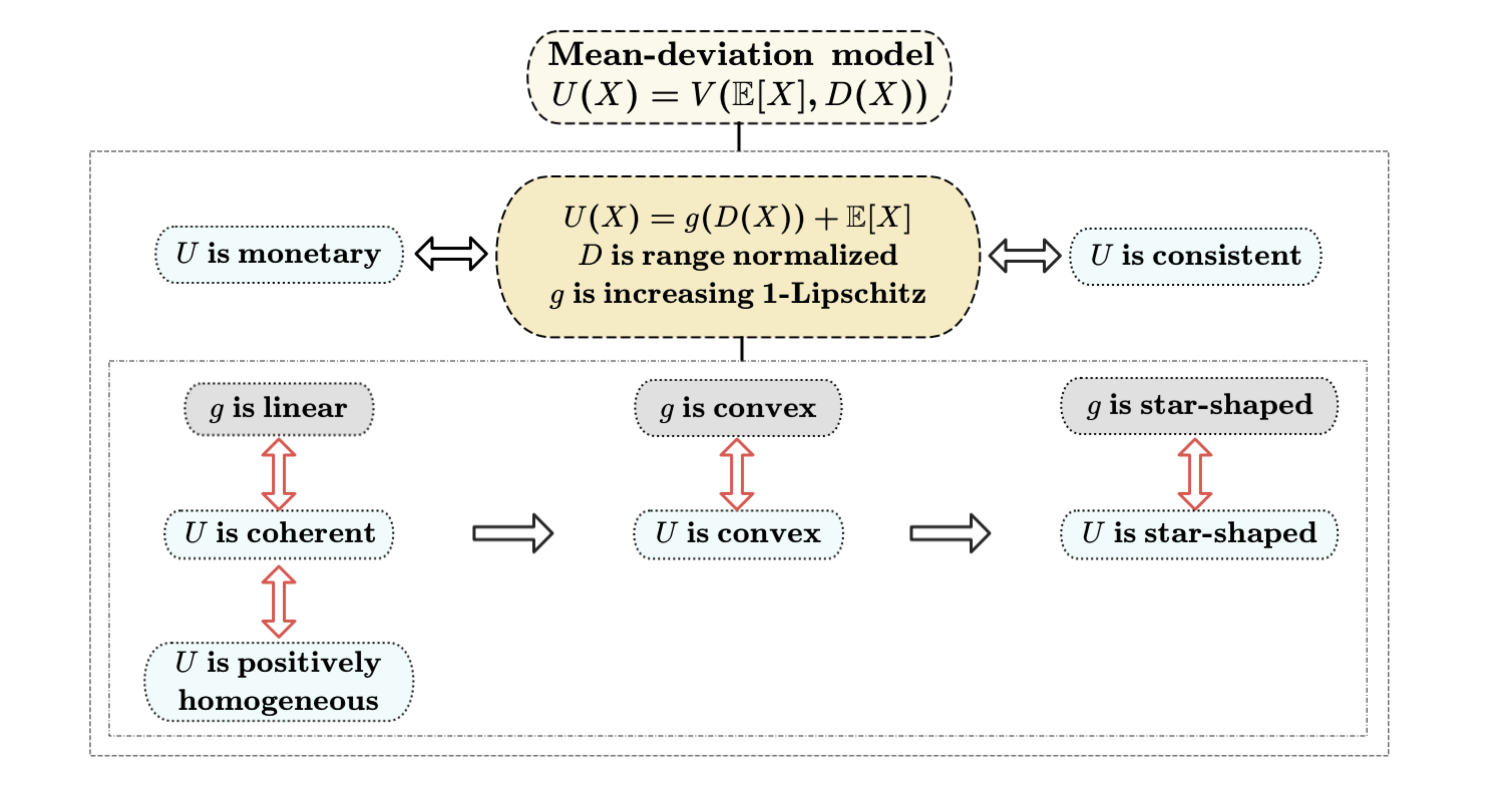
Figure 1: An illustration of properties of the mean-deviation model

In addition to proposing the mean-deviation measures in (4), our main contributions include a comprehensive study on this class of risk measures. In Section 4, an axiomatic foundation for $\mathrm{MD}^{D}_{g}$ (Theorem 2) is proposed based on results of Grechuk et al. (2012), and characterizations for coherent, convex or star-shaped risk measures are obtained in Theorem 3. We show that there is a one-to-one correspondence between $\mathrm{MD}^{D}_{g}$ and the risk-weighting function $g$, and hence the above classes can be identified based on properties of $g$. Figure 1 contains an illustration of properties of $\mathrm{MD}^{D}_{g}$. In particular, convexity of $g$ is equivalent to convexity of $\mathrm{MD}^{D}_{g}$. As a consequence, our structure offers new convex risk measures with explicit formulas, in addition to the existing convex distortion risk measures and entropy risk measures; see e.g., Dhaene et al. (2006), Laeven and Stadje (2013) and Föllmer and Schied (2016). Specifically, these formulas help us construct risk measures that are consistent yet not convex, or convex but not coherent (Theorem 3 and Proposition 2).

In Section 5, we specialize in the convex case of the monotonic mean-deviation measure and further study the dual representation of $\mathrm{MD}^{D}_{g}$ (Theorem 4), which is obtained directly through the conjugate function of $g$. In Section 6, we analyze worst-case values of $\mathrm{MD}^{D}_{g}$ under two popular settings to show its feasibility in model uncertainty problems (Propositions 4 and 5). In Section 7, when the deviation measures are the convex signed Choquet integral defined in Wang et al. (2020b), we discuss non-parametric estimation of $\mathrm{MD}^{D}_{g}$ (Theorem 5). The asymptotic normality and the asymptotic variance for the empirical estimators are obtained explicitly. These results yield an intuitive trade-off between statistical efficiency, in terms of estimation error, and sensitivity to risk, in terms of the risk-weighting function. We conclude the paper in Section 8. The supplement regarding the characterization of monotonicity in mean-deviation models is put in Appendix A, and the details in the axiomatization results are relegated to Appendix B. Appendix C provides a proof that is omitted from Section 7.

2 Preliminaries

Throughout this paper, we work with a nonatomic probability space $(\Omega,\mathcal{F},\mathbb{P})$. All equalities and inequalities of functionals on $(\Omega,\mathcal{F},\mathbb{P})$ are under $\mathbb{P}$ almost surely ($\mathbb{P}$-a.s.) sense. A risk measure $\rho$ is a mapping from $\mathcal{X}$ to $(-\infty,\infty]$, where $\mathcal{X}$ is a convex cone of random variables representing losses faced by financial institutions. We denote by $\mathbb{E}[X]$ the expectation of the random variable $X$. Let $X\in\mathcal{X}$ represent the random loss faced by financial institutions in a fixed period of time. That is, a positive value of $X\in\mathcal{X}$ represents a loss and a negative value represents a surplus in our sign convention, which is used by, e.g., McNeil et al. (2015). Further, denote by $\mathcal{X}^{\circ}$ the set of all nonconstant random variables in $\mathcal{X}$. Let $F_{X}$ be the distribution function of $X$, and we write $X\buildrel\mathrm{d}\over{=}Y$ if two random variables $X$ and $Y$ have the same distribution. Terms such as increasing or decreasing functions are in the non-strict sense. For $p\in[1,\infty)$, we denote by $L^{p}=L^{p}(\Omega,\mathcal{F},\mathbb{P})$ the set of all random variables $X$ such that $\|X\|_{p}=(\mathbb{E}[|X|^{p}])^{1/p}<\infty$. Furthermore, $L^{\infty}=L^{\infty}(\Omega,\mathcal{F},\mathbb{P})$ is the space of all essentially bounded random variables, and $L^{0}=L^{0}(\Omega,\mathcal{F},\mathbb{P})$ denotes the space of all random variables. When considering a mapping defined on $L^{p}$ for some $p\in[1,\infty]$, we refer to its continuity in the context of the $L^{p}$-norm.

We define the two important risk measures in banking and insurance practice. The Value-at-Risk ($\mathrm{VaR}$) at level $\alpha\in(0,1)$ is the functional $\mathrm{VaR}_{\alpha}:L^{0}\to\mathbb{R}$ defined by

$$\mathrm{VaR}_{\alpha}(X)=\inf\{x\in\mathbb{R}:\mathbb{P}(X\leqslant x)\geqslant\alpha\},$$

which is precisely the left $\alpha$-quantile of $X$. In some places, we also use $F^{-1}_{X}(\alpha)$ instead of $\mathrm{VaR}_{\alpha}(X)$ for convenience. The Expected Shortfall ($\mathrm{ES}$) at level $\alpha\in[0,1)$ is the functional $\mathrm{ES}_{\alpha}:L^{1}\to\mathbb{R}$ defined by

$$\mathrm{ES}_{\alpha}(X)=\frac{1}{1-\alpha}\int_{\alpha}^{1}\mathrm{VaR}_{s}(X)\mathrm{d}s.$$

Artzner et al. (1999) introduced coherent risk measures as those satisfying the following four properties.

• Monotonicity: $\rho(X)\leqslant\rho(Y)$ for all $X,Y\in\mathcal{X}$ with $X\leqslant Y$.

• Cash additivity: $\rho(X+c)=\rho(X)+c$ for all $c\in\mathbb{R}$ and $X\in\mathcal{X}$.

• Positive homogeneity: $\rho(\lambda X)=\lambda\rho(X)$ for all $\lambda\in(0,\infty)$ and $X\in\mathcal{X}$.

• Subadditivity: $\rho(X+Y)\leqslant\rho(X)+\rho(Y)$ for all $X,Y\in\mathcal{X}$.

ES satisfies all four properties above, whereas VaR does not satisfy [SA]. We say that $\rho$ is a monetary risk measure if it satisfies [M] and [CA]. Moreover, $\rho$ is a convex risk measure if it is monetary and further satisfies

• Convexity: $\rho(\lambda X+(1-\lambda)Y)\leqslant\lambda\rho(X)+(1-\lambda)\rho(Y)$ for all $X,Y\in\mathcal{X}$ and $\lambda\in[0,1]$.

Clearly, [PH] together with [SA] implies [Cx]. Risk measures satisfying [CA] and [Cx] but not [M] are studied by e.g., Filipović and Svindland (2008). For more discussions and interpretations of these properties, we refer to Föllmer and Schied (2016). Another class of risk measures is defined based on consistency with respect to second-order stochastic dominance (SSD):

1. SSD-consistency: $\rho(X)\leqslant\rho(Y)$ if $X\leqslant_{\rm SSD}Y$ (i.e., $\mathbb{E}[u(X)]\leqslant\mathbb{E}[u(Y)]$ for all increasing convex functions $u$).

Monetary risk measures satisfying [SC] are called consistent risk measures, and they are characterized by Mao and Wang (2020) as the infima of law-invariant convex risk measures (law-invariance is defined via (D5) below). The property [SC] is often called strong risk aversion for a preference functional in decision theory; see Rothschild and Stiglitz (1970). A related notion to SSD is convex order, also called mean-preserving spread, denoted by $X\leqslant_{\rm cx}Y$, meaning $X\leqslant_{\rm SSD}Y$ and $\mathbb{E}[X]=\mathbb{E}[Y]$.

In decision making, deviation measures are also introduced to measure the uncertainty inherent in a random variable, and are studied systematically for their application to risk management in areas like portfolio optimization and engineering. Such measures include standard deviation as a special case but need not be symmetric with respect to ups and downs. We give the definition of deviation measures in Rockafellar et al. (2006) below.

Definition 1 (Deviation measures).

Fix $p\in[1,\infty]$. A deviation measure is a functional $D:L^{p}\rightarrow[0,\infty)$ satisfying

• $D(X+c)=D(X)$ for all $X\in L^{p}$ and $c\in\mathbb{R}$.

• $D(X)>0$ for all $X\in(L^{p})^{\circ}$.

• $D(\lambda X)=\lambda D(X)$ for all $X\in L^{p}$ and $\lambda\geqslant 0$.

• $D(X+Y)\leqslant D(X)+D(Y)$ for all $X,Y\in L^{p}$.

Note that (D3) implies $D(0)=0$. We remark that the deviation measures in Rockafellar et al. (2006) is defined on $L^{2}$ since it is easy to access tools associated with duality. However, as mentioned in Rockafellar et al. (2006), this does not prevent us from working with the general $L^{p}$ norms for $p\in[1,\infty]$. Moreover, we will focus on law-invariant deviation measures, which further satisfy

• $D(X)=D(Y)$ for all $X,Y\in L^{p}$ if $X\stackrel{{\scriptstyle d}}{{=}}Y$.

We use $\mathcal{D}^{p}$ to denote the set of $D$ satisfying (D1)-(D5). Note that the combination of (D3) with (D4) implies that each $D\in\mathcal{D}^{p}$ is a convex functional. The law-invariant deviation measures include, for instance, standard deviation, semideviation, ES deviation and range-based deviation; see Examples 1 and 2 of Rockafellar et al. (2006) and Section 4.1 of Grechuk et al. (2012). Moreover, $D$ is called an upper range dominated deviation measure if it has the following property

$$D(X)\leqslant\mathrm{ess\mbox{-}sup}X-\mathbb{E}[X]\leavevmode\nobreak\ \leavevmode\nobreak\ \text{for all\leavevmode\nobreak\ }X\in L^{p},$$ (5)

where $\mathrm{ess\mbox{-}sup}X$ is the essential supremum of $X$. For more discussions and interpretations of the properties of deviation measures mentioned above, we refer to Rockafellar et al. (2006).

Deviation measures are not risk measures in the sense of Artzner et al. (1999), but the connection between deviation measures and risk measures is strong. It is shown in Theorem 2 of Rockafellar et al. (2006) that upper range bounded deviation measures $D$ correspond one-to-one with coherent, strictly expectation bounded risk measures $R$ with the relations that $D(X)=R(X)-\mathbb{E}[X]$ or $R(X)=D(X)+\mathbb{E}[X]$. Note that the additive structure $R=D+\mathbb{E}$ can be seen as a special form of the combination of mean and deviation. Below, we define a general mean-deviation model.

Definition 2 (Mean-deviation model).

Fix $p\in[1,\infty]$. For a deviation measure $D\in\mathcal{D}^{p}$, a mean-deviation model is a functional $U:L^{p}\rightarrow(-\infty,\infty]$ defined as

$$U(X)=V(\mathbb{E}[X],D(X)),$$ (6)

where $V:\mathbb{R}\times[0,\infty)\to(-\infty,\infty]$ satisfies (i) $V$ is increasing component-wise; (ii) $V(m,0)=m$ for all $m\in\mathbb{R}$; (iii) $V(m,d)$ is not determined only by $m$.

The three conditions on $V$ in Definition 2 are simple and intuitive. More specifically, (i) is the basic requirement that $U$ increases when the mean or deviation increases, with the other argument fixed; (ii) means that a constant random variable has risk value equal to itself; (iii) means that the model is not trivial in the sense that it does not ignore the deviation $D(X)$. Our definition is different from that of Grechuk et al. (2012), who required further strict monotonicity of $V$ with a real-valued range. Therefore, our requirement is weaker than Grechuk et al. (2012), and this relaxation allows us to include the most popular models of Markowitz (1952) in (2), that is,

$$V(\mathbb{E}[X],\mathrm{SD}(X))=V_{\sigma}(\mathbb{E}[X],\mathrm{Var}(X))=\mathbb{E}[X]+\infty\times\mathds{1}_{\{\mathrm{SD}(X)>\sigma\}},$$

which is neither strictly increasing nor real-valued. Here we use $\mathrm{SD}$ (the standard deviation) instead of $\mathrm{Var}$ because $\mathrm{SD}\in\mathcal{D}^{2}$.

As mentioned in Introduction, the mean-deviation model has many nice properties; however, it is not necessarily monotonic or cash additive in general, and thus is not a monetary risk measure. Grechuk et al. (2012) provided an axiomatic framework for the mean-deviation model via the preference relation by further assuming some other properties; but it does not belongs to the class of monetary risk measures. Han et al. (2023) characterized mean-deviation models with $D=\mathrm{ES}_{\alpha}-\mathbb{E}$ for $\alpha\in(0,1)$ by extending axioms for ES in Wang and Zitikis (2021), which can be further required to be monetary. Since [M] and [CA] are common in the literature of decision theory and risk measures, and they correspond to the interpretation of a risk measure as regulatory capital requirement, it is natural to further consider general conditions for a mean-deviation model to be monetary. This leads to the main object of this paper, monotonic mean-deviation measures, formally introduced in the next section.

3 Monotonic mean-deviation measures

We first define monotonic mean-deviation measures. For this, we write

$$\overline{\mathcal{D}}^{p}=\left\{D\in\mathcal{D}^{p}:\sup_{X\in{(L^{p})}^{\circ}}\frac{D(X)}{\mathrm{ess\mbox{-}sup}X-\mathbb{E}[X]}=1\right\}.$$

Deviation measures in $\overline{\mathcal{D}}^{p}$ are called range normalized. For $\lambda>0$, a real function $g$ is $\lambda$-Lipschitz if

$$|g(x)-g(y)|\leqslant\lambda|x-y|\leavevmode\nobreak\ \leavevmode\nobreak\ \mbox{ for}\leavevmode\nobreak\ x,y\mbox{\leavevmode\nobreak\ in the domain of $g$}.$$ (7)

Definition 3.

Fix $p\in[1,\infty]$ and let $D\in\overline{\mathcal{D}}^{p}$. A monotonic mean-deviation measure $\mathrm{MD}^{D}_{g}:{L}^{p}\to\mathbb{R}$ is defined by

$$\mathrm{MD}^{D}_{g}(X)=g(D(X))+\mathbb{E}[X],$$ (8)

where $g:[0,\infty)\rightarrow\mathbb{R}$ is a non-constant increasing and $1$-Lipschitz function satisfying $g(0)=0$, called a risk-weighting function. We use $\mathcal{G}$ to denote the set of such functions $g$.

The interpretation of $g$ should be self-evident: it dictates how $D(X)$ is reflected in the calculation of $\mathrm{MD}^{D}_{g}$, and it is a generalization of the risk-weighting parameter $\lambda$ in $\mathbb{E}+\lambda D$, hence the name. We will establish explicit one-to-one correspondence between properties of the risk measure $\mathrm{MD}^{D}_{g}$ and properties of the risk-weighting function $g$ in the next section. The reason of requiring the conditions $D\in\overline{\mathcal{D}}^{p}$ and $g\in\mathcal{G}$ in Definition 3 will be justified in Theorem 1 below, which shows that these conditions are necessary and sufficient for (8) to be monetary, up to normalization of $D$ by scaling.

Theorem 1.

Fix $p\in[1,\infty]$. Suppose that $U:L^{p}\to(-\infty,\infty]$ is a mean-deviation model in (6) with $D\in{\mathcal{D}}^{p}$. The following statements are equivalent.

• $U$ is a monetary risk measure.

• $U$ is a consistent risk measure.

• For some $\lambda>0$, $\lambda D\in\overline{\mathcal{D}}^{p}$ and $U=g\circ D+\mathbb{E}$ where $g:[0,\infty)\rightarrow\mathbb{R}$ is a non-constant increasing and $\lambda$-Lipschitz function satisfying $g(0)=0$.

Proof.

(ii) $\Rightarrow$ (i) is trivial.

(iii) $\Rightarrow$ (ii): Without loss of generality we can take $\lambda=1$. The property of [CA] is clear. Next, we show the property of [M]. For any $X,Y\in L^{p}$ with $X\leqslant Y$, if $D(Y)\geqslant D(X)$, it is obviously to see that $U(X)\leqslant U(Y)$. Assume now $D(X)>D(Y)$. It holds that

$$U(Y)-U(X)=g(D(Y))+\mathbb{E}[Y]-g(D(X))-\mathbb{E}[X]\geqslant D(Y)-D(X)+\mathbb{E}[Y]-\mathbb{E}[X],$$

where we have used the $1$-Lipschitz condition of $g$ in the inequality. Since $D\in\overline{\mathcal{D}}^{p}$, it follows from Theorem 2 of Rockafellar et al. (2006) that there exists one-to-one correspondence with coherent risk measures denoted by $R$ in the relation that $R(X)=D(X)+\mathbb{E}[X]$ for $X\in L^{p}$. The monotoicity of $R$ implies that

$$U(Y)-U(X)\geqslant D(Y)-D(X)+\mathbb{E}[Y]-\mathbb{E}[X]=R(Y)-R(X)\geqslant 0.$$

Hence, we have verified [M] of $U$.

It remains to show that $U$ satisfies [SC]. Since $D$ is continuous and further satisfies convexity, law-invariance and the space is nonatomic, we have that $D$ is consistent with respect to convex order (see, e.g., Theorem 4.1 of Dana (2005)). Noting that $g$ is increasing, we have $U$ is also consistent with respect to convex order. Combining with [M] of $U$, it follows from Theorem 4.A.6 of Shaked and Shanthikumar (2007) that $U$ satisfies [SC]. This completes the proof of (iii) $\Rightarrow$ (ii).

(i) $\Rightarrow$ (iii): Define $g(d)=V(0,d)$ for $d\geqslant 0$. It is clear that $g$ is an increasing function with $g(0)=V(0,0)=0$. By [CA], we have

$$U(X) =U(X-\mathbb{E}[X])+\mathbb{E}[X]$$

$$=V(0,D(X))+\mathbb{E}[X]=g(D(X))+\mathbb{E}[X].$$

By Lemma 1 below, we have $\lambda D\in\overline{\mathcal{D}}^{p}$ for some $\lambda>0$. It remains to show that $g$ is $\lambda$-Lipschitz. Denote by $k=1/\lambda$. Since $\lambda D\in\overline{\mathcal{D}}^{p}$, for any $\varepsilon\in(0,k)$, there exists $X_{1}$ such that

$$k-\varepsilon<\frac{D(X_{1})}{\mathrm{ess\mbox{-}sup}X_{1}-\mathbb{E}[X_{1}]}\leqslant k.$$

For any $a>0$ and $d\geqslant 0$, define

$$X_{2}=a\frac{X_{1}-\mathrm{ess\mbox{-}sup}X_{1}}{\mathrm{ess\mbox{-}sup}X_{1}-\mathbb{E}[X_{1}]}\leavevmode\nobreak\ \leavevmode\nobreak\ \text{and}\leavevmode\nobreak\ \leavevmode\nobreak\ X_{3}=\frac{d}{a}X_{2}+d.$$

It is obvious that $\mathbb{E}[X_{2}]=-a,X_{2}\leqslant 0$ and $\mathbb{E}[X_{3}]=0.$ Moreover, $a(k-\varepsilon)<D(X_{2})\leqslant ak$ and $d(k-\varepsilon)<D(X_{3})\leqslant dk$. Also, $\mathbb{E}[X_{2}+X_{3}]=-a$ and $(d+a)(k-\varepsilon)<D(X_{2}+X_{3})\leqslant(d+a)k$. Since $X_{2}+X_{3}\leqslant X_{3}$, by [M], we have $g(D(X_{2}+X_{3}))+\mathbb{E}[X_{2}+X_{3}]\leqslant g(D(X_{3}))+\mathbb{E}[X_{3}]$. Letting $\varepsilon\to 0$, we conclude that $g_{-}((d+a)k)\leqslant g(dk)+a$, where $g_{-}(x)=\lim_{y\uparrow x}g(y)$ for all $x\geqslant 0$. This is equivalent to $g_{-}(d+a)-g(d)\leqslant\lambda a$ for any $a>0$ and $d\geqslant 0$. Note that $g$ is increasing. We have that $g:[0,\infty)\to\mathbb{R}$ is $\lambda$-Lipschitz. This completes the proof. ∎

In the proof of Theorem 1, the following result is needed.

Lemma 1.

Fix $p\in[1,\infty]$, and let $D\in\mathcal{D}^{p}$. If $U=V(\mathbb{E},D)$ in (6) satisfies [M], then we have $U(X)<\infty$ for all $X\in L^{p}$, and there exists $\lambda>0$ such that $\lambda D\in\overline{\mathcal{D}}^{p}$.

Proof.

To show that $U(X)$ is finite, take $Y\in L^{\infty}$ such that $\mathbb{E}[Y]=\mathbb{E}[X]$ and $D(Y)=D(X)$. Such $Y$ exists because $D$ is positively homogeneous. Therefore, $U(X)=U(Y)\leqslant U(\mathrm{ess\mbox{-}sup}Y)=V(\mathrm{ess\mbox{-}sup}Y,0)=\mathrm{ess\mbox{-}sup}Y<\infty.$

We next prove

$$K:=\sup_{X\in{(L^{p})}^{\circ}}\frac{D(X)}{\mathrm{ess\mbox{-}sup}X-\mathbb{E}[X]}<\infty.$$ (9)

by contradiction, which is equivalent to $\lambda D\in\overline{\mathcal{D}}^{p}$ with $\lambda=1/K$. Assume that $K=\infty$ in (9). For $X_{1},X_{2}\in L^{p}$ such that $\mathbb{E}[X_{1}]<\mathbb{E}[X_{2}]$, let $m_{1}=\mathbb{E}[X_{1}]$, $d_{1}=D(X_{1})$, $m_{2}=\mathbb{E}[X_{2}]$, $d_{2}=D(X_{2})$, and $e=m_{2}-m_{1}$. If $K=\infty$, there exists $Y_{1}$ such that ${D\left(Y_{1}\right)}/{(\mathrm{ess\mbox{-}sup}Y_{1}-\mathbb{E}[Y_{1}])}\geqslant{d_{1}}/{e}.$ Denote by $Y_{2}=e{(Y_{1}-\mathrm{ess\mbox{-}sup}Y_{1})}/{(\mathrm{ess\mbox{-}sup}Y_{1}-\mathbb{E}[Y_{1}])}+m_{2}.$ It holds that $\mathbb{E}\left[Y_{2}\right]=-e+m_{2}=m_{1}$ and ${D}\left(Y_{2}\right)\geqslant d_{1}$, and thus $U(X_{1})=V(m_{1},d_{1})\leqslant V(\mathbb{E}[Y_{2}],D(Y_{2}))=U(Y_{2})$. On the other hand, observe that $Y_{2}\leqslant m_{2}$. Consequently, by monotonicity, we have $U(Y_{2})\leqslant U(m_{2})$. Thus, we have $U(X_{1})\leqslant U(Y_{2})\leqslant U(m_{2})\leqslant U(X_{2}),$ which implies that $U(X)\leqslant U(Y)$ for every $X$ and $Y$ with $\mathbb{E}[X]<\mathbb{E}[Y]$. Hence,

$$\mathbb{E}[X]-\varepsilon=U(\mathbb{E}[X]-\varepsilon)\leqslant U(X)\leqslant U(\mathbb{E}[X]+\varepsilon)=\mathbb{E}[X]+\varepsilon$$

for any $X\in\ L^{p}$ and $\varepsilon>0$. Letting $\varepsilon\downarrow 0$ yields $U(X)=\mathbb{E}[X]$, contradicting (iii) in Definition 2. Therefore, we conclude $K<\infty.$ This completes the proof. ∎

Note that if $D$ and $g$ satisfy the conditions in Theorem 1 (iii), then there exists $\widetilde{D}\in\overline{\mathcal{D}}^{p}$ and $\widetilde{g}\in\mathcal{G}$ such that $\widetilde{g}\circ\widetilde{D}=g\circ D$. Therefore, Definition 2 includes all possible choices of mean-deviation models satisfying [M] and [CA].

Lemma 1 provides a necessary condition for [M] on the mean-deviation model. For the sake of completeness, we will elaborate on the characterization of [M], under the assumption that this necessary condition is met; this is detailed in Appendix A. Lemma 1 also implies in particular that we can limit the range of the mean-deviation model to $\mathbb{R}$ when [M] is imposed.

For a deviation measure defined on $L^{p}$, the condition that $\lambda D\in\overline{\mathcal{D}}^{p}$ for some $\lambda>0$ in Lemma 1 is called weakly upper-range dominated by Grechuk et al. (2012). It is clear from (5) that every upper-range dominated deviation measure is weakly upper-range dominated with $\lambda\geqslant 1$. In particular, if $D$ takes the form of $\mathrm{ES}_{\alpha}-\mathbb{E}$ with $\alpha\in(0,1)$, $\mathrm{ess\mbox{-}sup}X-\mathbb{E}[X]$ or $\mathbb{E}[|X-\mathbb{E}[X]|]/2$, we have $D\in\overline{\mathcal{D}}^{p}$ (see Example 5 of Grechuk et al. (2012) for the last one). Examples of deviation measures $D$ satisfying $\lambda D\in\overline{\mathcal{D}}^{p}$ for some $\lambda>0$ also include the mean-absolute deviation, the Gini deviation, the inter-ES range, and the inter-expectile range (for the last two, see Bellini et al. (2022)).

Note that $R=D+\mathbb{E}$ is a finite coherent risk measure on $L^{p}$ for any $D\in\overline{\mathcal{D}}^{p}$. It follows that $R$ is continuous (see e.g., Corollary 2.3 of Kaina and Rüschendorf (2009)). Consequently, this implies that a range-normalized deviation measure is always continuous. Below we characterize the class of range-normalized deviation measures by elucidating the relationship between coherent risk measures and the deviation measures in $\overline{D}^{p}$.

Proposition 1.

Fix $p\in[1,\infty]$. The deviation measure $D\in\mathcal{D}^{p}$ is range normalized if and only if $D+\mathbb{E}$ is a coherent risk measure and $\lambda D+\mathbb{E}$ is not a coherent risk measure for $\lambda>1$.

Proof.

The necessity follows immediately from Theorem 2 of Rockafellar et al. (2006) since $D\in\overline{\mathcal{D}}^{p}$ is upper range dominated (see (5) for the definition) and $\lambda D$ is not upper range dominated for any $\lambda>1$. Conversely, we assume by contradiction that $D$ is not range normalized. Then, either $kD\in\overline{\mathcal{D}}^{p}$ for some $k>1$ or $kD\in\overline{\mathcal{D}}^{p}$ for some $k<1$ holds. In the first case, there exists $\lambda>1$ such that $\lambda D$ is upper range dominated. Applying Theorem 2 of Rockafellar et al. (2006), we have $\lambda D+\mathbb{E}$ is a coherent risk measure, thereby leading to a contradiction. In the second case, it holds that $D+\mathbb{E}$ is not a coherent risk measure since $D$ is not upper range dominated, which also yields a contradiction. ∎

The expected return maximization with variance constraint of Markowitz (1952) has the form $\mathrm{MD}_{g}^{D}$ where $D=\mathrm{SD}$ and $g(d)=\infty\times\mathds{1}_{\{d>\sigma\}}$ for some $\sigma>0$ as in (2). In this example, $g$ is not real-valued. Therefore, although sharing the form (8), $\mathrm{MD}_{g}^{D}$ is not a monotonic mean-deviation measure. Similarly, for $\lambda>0$, the functional $\mathrm{MD}_{g}^{D}(X)=\lambda(\mathrm{SD}(X))^{2}+\mathbb{E}[X]$ in (3) or $\mathrm{MD}_{g}^{D}(X)=\lambda\mathrm{SD}(X)+\mathbb{E}[X]$ is not a monotonic mean-deviation measure, because $\mathrm{SD}$ does not satisfies (9) for any $p\in[1,\infty]$. Nevertheless, in all three examples, $g$ is convex. Indeed, convexity of $g$ has important implications, and this will be studied in Section 4.2 below.

4 Characterization

4.1 Axiomatization of monotonic mean-deviation measures

We first present an axiomatization of the monotonic mean-deviation measure $\mathrm{MD}^{D}_{g}$ through preference relations. This axiomatization is very similar to Grechuk et al. (2012), who axiomatized preferences represented by a monotone functional $X\mapsto V(\mathbb{E}[X],D(X))$ for some strictly increasing function $V$. We relegate all details, including all proofs and a comparison with Grechuk et al. (2012), to Appendix B. Our main purpose here is to show that $\mathrm{MD}^{D}_{g}$ has an axiomatic foundation.

A preference relation $\succeq$ is defined by a total preorder. As usual, $\succ$ and $\simeq$ correspond to the antisymmetric and equivalence relations, respectively. For two random losses $X,Y$, the relation $X\succeq Y$ indicates that $X$ is preferred over $Y$, or equivalently, that $Y$ is considered more dangerous than $X$. A numerical representation of a preference $\succeq$ is a mapping $\rho:\mathcal{X}\rightarrow\mathbb{R}$, such that $X\succeq Y\Longleftrightarrow\rho(X)\leqslant\rho(Y)$. Note that $\succeq$ can be represented by a mapping $\rho$ if $\succeq$ is separable; see e.g., Drapeau and Kupper (2013). We use the following axioms, where all random variables are tacitly assumed to be in $L^{p}$ for some fixed $p\in[1,\infty]$.

• (Monotonicity). If $X_{1}\leqslant X_{2},$ then $X_{1}\succeq X_{2}$.

• (Translation-invariance). For any $c\in\mathbb{R}$, $X\succeq Y$ if and ony if $X+c\succeq Y+c$.

• (Weak positive homogeneity). If $\mathbb{E}[X]=\mathbb{E}[Y]$ and $X\succeq Y$, then $\lambda X\succeq\lambda Y$ for any $\lambda>0$.

• (Risk aversion). If $X\leqslant_{\rm cx}Y$, then $X\succeq Y$. In addition, $\mathbb{E}[X]\succ X$ for any non-constant $X$.

• (Solvability). There exists $c\in\mathbb{R}$ such that $X\simeq c$.

• (Weak convexity). If $\mathbb{E}[X]=\mathbb{E}[Y]$ and $X\simeq Y$, then $\lambda X+(1-\lambda)Y\succeq X$ for all $\lambda\in[0,1]$.

• (Continuity). For every $X$, the sets $\left\{Y\in L^{p}:Y\succeq X\right\}$ and $\left\{Y\in L^{p}:X\succeq Y\right\}$ are $L^{p}$-closed.

These axioms are standard, and we refer to Yaari (1987), Drapeau and Kupper (2013), Föllmer and Schied (2016, Chapeter 2) and Grechuk et al. (2012) for interpretations and discussions of these axioms. The following result gives an axiomatization of $\mathrm{MD}^{D}_{g}$ in Definition 3.

Theorem 2.

Fix $p\in[1,\infty]$. A preference $\succeq$ on $L^{p}$ satisfies Axioms A1–A7 if and only if $\succeq$ can be represented by $\mathrm{MD}^{D}_{g}=g\circ D+\mathbb{E}$ for some $D\in\overline{\mathcal{D}}^{p}$ and $g\in\mathcal{G}$ that is strictly increasing.

Grechuk et al. (2012) obtained a representation with the form $X\mapsto V(\mathbb{E}[X],D(X))$ using a weak translation-invariant property, and the mean-deviation model is not cash-additive. Our stronger version of translation-invariance pins down the more explicit form of monotonic mean-deviation measures. For the detailed differences between our axiomatization and that of Grechuk et al. (2012), see Appendix B. A subtle difference between Theorem 2 and Definition 3 is that $g$ is strictly increasing in Theorem 2 but not necessarily so in Definition 3. An axiomatization of $\mathrm{MD}^{D}_{g}$ with $g$ not necessarily strictly increasing is an open question, as we were not able to identify proper relaxations of the proposed axioms.

4.2 Characterizations of convex and coherent risk measures

In this subsection, we continue to study properties of $\mathrm{MD}^{D}_{g}$. Specifically, we characterize $g$ such that $\mathrm{MD}^{D}_{g}$ belongs to the class of coherent risk measures or convex risk measures. Moreover, we consider star-shaped risk measures, which are monetary risk measures $\rho$ further satisfying

• Star-shapedness: $\rho(0)=0$ and $\rho(\lambda X)\leqslant\lambda\rho(X)$ for all $X\in\mathcal{X}$ and $\lambda\in[0,1]$.

Similarly, a function $g:[0,\infty)\to\mathbb{R}$ is star-shaped if $g(0)=0$ and $g(\lambda x)\leqslant\lambda g(x)$ for all $x\in[0,\infty)$ and $\lambda\in[0,1]$. Star-shaped risk measures are characterized by Castagnoli et al. (2022) as the infimum of normalized (i.e., $\rho(0)=0$) convex risk measures. Under normalization, star-shapedness is weaker than both convexity and positive homogeneity.

Theorem 3.

Suppose that $D\in\overline{\mathcal{D}}^{p}$ for $p\in[1,\infty]$ and $g\in\mathcal{G}$. The following statements hold.

1. $\mathrm{MD}^{D}_{g}$ is a coherent risk measure if and only if $g$ is linear.

2. $\mathrm{MD}^{D}_{g}$ is a convex risk measure if and only if $g$ is convex.

3. $\mathrm{MD}^{D}_{g}$ is a star-shaped risk measure if and only if $g$ is star-shaped.

Proof.

(i) Sufficiency is straightforward. To show necessity, let $X$ be such that $\mathbb{E}[X]=0$ and $D(X)=1$; such $X$ exists due to Property (D3). Coherence of $\mathrm{MD}^{D}_{g}$ implies that for all $x>0$,

$$g(x)=\mathrm{MD}^{D}_{g}(xX)=x\mathrm{MD}^{D}_{g}(X)=xg(1).$$

This implies that $g$ is linear.

(ii) To see sufficiency, if $g$ is convex, then $\mathrm{MD}^{D}_{g}$ is a convex risk measure because expectation is linear and $D$ is convex. To show necessity, take $x,y\geqslant 0$ and $\lambda\in[0,1]$. Let $X$ be such that $\mathbb{E}[X]=0$ and $D(X)=1$. Since $\mathrm{MD}^{D}_{g}$ is convex and $D$ satisfies (D3), we have

$$g(\lambda x+(1-\lambda)y) =g\circ D((\lambda x+(1-\lambda)y)X)$$

$$=\mathrm{MD}^{D}_{g}((\lambda x+(1-\lambda)y)X)$$

$$\leqslant\lambda\mathrm{MD}^{D}_{g}(xX)+(1-\lambda)\mathrm{MD}^{D}_{g}(yX)=\lambda g(x)+(1-\lambda)g(y).$$

Thus, $g$ is convex.

(iii) To see sufficiency, if $g$ is star-shaped, then ${\rm MD}_{g}^{D}$ is star-shaped because expectation is linear and $D$ satisfies (D3). Conversely, let $X$ be such that $\mathbb{E}[X]=0$ and $D(X)=1$. For any $x\in[0,\infty)$ and $\lambda\in[0,1]$, it follows from the star-shapedness of ${\rm MD}_{g}^{D}$ that $g(0)={\rm MD}_{g}^{D}(0)=0$ and

$$g(\lambda x)={\rm MD}_{g}^{D}(\lambda xX)\leqslant\lambda{\rm MD}_{g}^{D}(xX)=\lambda g(x).$$

This implies that $g$ is star-shaped. ∎

By Theorem 3 (i), $\mathrm{MD}^{D}_{g}$ is coherent if and only if

$$\mathrm{MD}^{D}_{g}(X)=\lambda D(X)+\mathbb{E}[X]=\lambda R(X)+(1-\lambda)\mathbb{E}[X],\leavevmode\nobreak\ \leavevmode\nobreak\ X\in L^{p}$$

for some $\lambda\in[0,1]$, where $R=D+\mathbb{E}$ is a coherent risk measure. In fact, positive homogeneity of $\mathrm{MD}^{D}_{g}$ is sufficient for $g$ to be linear, as seen from the proof of (i). Therefore, for $\mathrm{MD}^{D}_{g}$, positive homogeneity and coherence are equivalent. Moreover, following the same proof, the result in (ii) can be strengthened to a more general form without monotonicity: For any function $g:[0,\infty)\to\mathbb{R}$ and $D\in\mathcal{D}^{p}$ with $p\in[1,\infty]$, we have that $\mathrm{MD}^{D}_{g}$ is convex if and only if $g$ is convex.

For the special choice of $D=\mathrm{ES}_{\alpha}-\mathbb{E}$ where $\alpha\in(0,1)$, Han et al. (2023) obtained characterizations for $\mathrm{MD}^{D}_{g}$ to be coherent, convex, or consistent risk measures. Theorem 3 extends this result to deviation measures. Our results allow for explicit formulas for many consistent risk measures that are not convex. In contrast, existing examples of consistent but non-convex risk measures are often obtained by taking an infimum over convex risk measures.

In the following proposition, we obtain an alternative representation result for $\mathrm{MD}^{D}_{g}$ when $g$ is convex.

Proposition 2.

Fix $p\in[1,\infty]$. For $g\in\mathcal{G}$ and $D\in\overline{\mathcal{D}}^{p}$, $\mathrm{MD}^{D}_{g}$ is a convex risk measure if and only if

$$\mathrm{MD}^{D}_{g}(X)=\lambda\mathbb{E}[(D(X)-Y)_{+}]+\mathbb{E}[X]$$ (10)

for some non-negative random variable $Y\in L^{1}$ and some constant $\lambda\in[0,1]$. In particular, $\mathrm{MD}^{D}_{g}$ is a coherent risk measure if and only if $Y=0$.

Proof.

We need to show that $g$ is an increasing, convex function which satisfies $1$-Lipschitz condition if and only if $g(x)=\lambda\mathbb{E}[(x-Y)_{+}]$ for some $Y\geqslant 0$ and $0\leqslant\lambda\leqslant 1$. This is known in the literature; see Theorems 1 and 6 of Williamson (1956). ∎

By Theorem 1, we know that $\mathrm{MD}^{D}_{g}$ is a consistent risk measure, yet it fails to exhibit convexity when $g\in\mathcal{G}$ is not convex as shown in Theorem 3. For instance, take $g(x)=\lambda\mathbb{E}[x\wedge Y]$ for some non-negative $Y$ and $\lambda\in[0,1]$. It is obvious that $g$ is concave and satisfies $1$-Lipschitz condition. In this case, $\mathrm{MD}^{D}_{g}(X)$ can be expressed as

$$\mathrm{MD}^{D}_{g}(X)=\lambda\mathbb{E}[D(X)\wedge Y]+\mathbb{E}[X],$$

which is a consistent but not convex risk measure. Furthermore, Theorem 3 illustrates that $\mathrm{MD}^{D}_{g}$ is a convex but not coherent risk measure if $g\in\mathcal{G}$ is convex yet non-linear. This insight opens up a new perspective for constructing risk measures within the class of monotone mean-deviation risk measures. Specifically, it guides us in developing risk measures that are consistent yet not convex, or alternatively, convex but not coherent, all while possessing an explicit formulation. By assuming that $g(x)=\mathbb{E}[(x-Y)_{+}]$ or $g(x)=\mathbb{E}[x\wedge Y]$ for some non-negative random variable $Y$, we can construct many convex or consistent risk measures with explicit form which appear to be new in the literature.

Example 1.

Suppose that $g(x)=\mathbb{E}[(x-Y)_{+}]$ for some $Y\geqslant 0$ and $D\in\overline{\mathcal{D}}^{p}$ with some $p\in[1,\infty]$.

1. Let $Y$ be the exponential distribution with parameter $\beta>0$, that is, $\mathbb{P}(Y>y)=e^{-\beta y}$, then $g(x)=x+\left(e^{-\beta x}-1\right)/{\beta}$. According to Proposition 2, we have

   $$\rho(X)=\mathbb{E}[X]+D(X)+\frac{1}{\beta}\left(e^{-\beta D(X)}-1\right),$$

   which is a convex risk measure.

2. Let $Y$ follow a Pareto distribution with tail parameter $\theta>0$, that is, $\mathbb{P}(Y>y)=(1+y)^{-\theta}$ for $y\geqslant 0$. We have

   $$g(x)=\left\{\begin{aligned} &x+\left((1+x)^{1-\theta}-1\right)/{(\theta-1)},&\theta\neq 1,\\ &x-\log(1+x),&\theta=1.\end{aligned}\right.$$

   This yields

   $$\rho(X)=\left\{\begin{aligned} &\mathbb{E}[X]+D(X)+\left(\left(1+D(X)\right)^{1-\theta}-1\right)/(\theta-1),&\theta\neq 1,\\ &\mathbb{E}[X]+D(X)-\log(1+D(X)),&\theta=1,\end{aligned}\right.$$

   and $\rho$ is a convex risk measure.

Example 2.

Suppose that $g(x)=\mathbb{E}[x\wedge Y]$ for some $Y\geqslant 0$ and $D\in\overline{\mathcal{D}}^{p}$ for some $p\in[1,\infty]$.

1. Let $Y$ follow the exponential distribution with parameter $\beta>0$, we have $g(x)=\left(1-e^{-\beta x}\right)/\beta$. Then it follows that

   $$\rho(X)=\mathbb{E}[X]+\frac{1}{\beta}\left(1-e^{-\beta D(X)}\right),$$

   which is a consistent risk measure but not a convex risk measure.

2. Let $Y$ follow a Pareto distribution with tail parameter $\theta>0$. We have

   $$g(x)=\left\{\begin{aligned} &\left(1-(1+x)^{1-\theta}\right)/{(\theta-1)},&\theta\neq 1,\\ &\log(1+x),&\theta=1.\end{aligned}\right.$$

   This yields

   $$\rho(X)=\left\{\begin{aligned} &\mathbb{E}[X]+\frac{1-(1+D(X))^{1-\theta}}{\theta-1},&\theta\neq 1,\\ &\mathbb{E}[X]+\log(1+D(X)),&\theta=1,\end{aligned}\right.$$

   which is a consistent risk measure but not a convex risk measure.

5 Dual representation

In this section, we investigate the dual representation of monotonic deviation measures that are convex. Before showing the main result, we need some preliminaries. For $p\in[1,\infty)$, denote by $q$ the conjugate dual of $p$, i.e., $q=(1-1/p)^{-1}$. Define $\mathcal{A}_{p}=\{Z\in L^{q}:Z\geqslant 0,\leavevmode\nobreak\ \mathbb{E}[Z]=1\}$. For a convex $g\in\mathcal{G}$, we use $g^{*}$ to represent its conjugate function, i.e., $g^{*}(y)=\sup_{x\geqslant 0}\{xy-g(x)\}$. One can easily check that $g^{*}$ is increasing, convex and lower semicontinuous. Note that $g:[0,\infty)\to\mathbb{R}$ is increasing and $1$-Lipschitz continuous with $g(0)=0$. Denote by $a=\lim_{x\to\infty}g^{\prime}(x)\in[0,1]$ where $g^{\prime}$ is the left derivative of $g$, and we have $g^{*}(y)=0$ for $y\leqslant 0$ and $g^{*}(y)=\infty$ for $y>a$. Hence, it holds that $g(x)=g^{**}(x)=\sup_{y\in[0,a]}\{xy-g^{*}(y)\}$ for $x\geqslant 0$ (see e.g., Proposition A.6 of Föllmer and Schied (2016)). For a range-normalized deviation measure $D$, denote by $R=D+\mathbb{E}$, which is a finite coherent risk measure on $L^{p}$. Moreover, the following representation holds:

$$R(X)=D(X)+\mathbb{E}[X]=\max_{Z\in\mathcal{A}}\mathbb{E}[XZ],\leavevmode\nobreak\ \leavevmode\nobreak\ X\in L^{p}$$ (11)

for some convex and weakly compact set $\mathcal{A}\subseteq\mathcal{A}_{p}$.

Theorem 4.

Fix $p\in[1,\infty)$. Suppose that $g\in\mathcal{G}$ is convex with $\lim_{x\to\infty}g^{\prime}(x)=a$ and $D\in\mathcal{\overline{D}}^{p}$. We have

$$\mathrm{MD}^{D}_{g}(X)=\max_{Z\in\mathcal{A}}\left\{a\mathbb{E}[XZ]-g^{*}\left(\frac{a}{\sup\{\lambda\in[1,\infty):\lambda(Z-1)+1\in\mathcal{A}\}}\right)\right\}+(1-a)\mathbb{E}[X],\leavevmode\nobreak\ \leavevmode\nobreak\ X\in L^{p},$$

where $\mathcal{A}$ is defined in (11).

Proof.

By Theorem 3, ${\rm MD}^{D}_{g}$ is a finite convex risk measure on $L^{p}$. It follows from Theorem 2.11 of Kaina and Rüschendorf (2009) that

$$\mathrm{MD}^{D}_{g}(X)=\max_{Z\in\mathcal{A}_{p}}\{\mathbb{E}[XZ]-\beta(Z)\},\leavevmode\nobreak\ \leavevmode\nobreak\ X\in L^{p},$$

for some $\beta:L^{q}\to(-\infty,\infty]$ that is convex and lower semicontinuous, given by

$$\beta(Z)=\sup_{X\in L^{p}}\{\mathbb{E}[XZ]-\mathrm{MD}^{D}_{g}(X)\},\leavevmode\nobreak\ \leavevmode\nobreak\ Z\in L^{q}.$$

We first aim to prove that

$$\beta(Z)=\begin{cases}g^{*}\left(\frac{1}{\sup\{\lambda\in[1/a,\infty):\lambda(Z-1)+1\in\mathcal{A}\}}\right),\leavevmode\nobreak\ \leavevmode\nobreak\ &Z\in\mathcal{Z},\\ \infty,\leavevmode\nobreak\ \leavevmode\nobreak\ &{\rm otherwise},\end{cases}$$ (12)

where $\mathcal{Z}=\{aY+1-a:Y\in\mathcal{A}\}$. For $Z\in L^{q}$, we have

$$\beta(Z) =\sup_{X\in L^{p}}\{\mathbb{E}[XZ]-\mathrm{MD}^{D}_{g}(X)\}$$

$$=\sup_{X\in L^{p}}\{\mathbb{E}[XZ]-\mathbb{E}[X]-g(D(X))\}$$

$$=\sup_{X\in L^{p}}\inf_{y\in[0,a]}\{\mathbb{E}[XZ]-\mathbb{E}[X]-D(X)y+g^{*}(y)\},$$ (13)

where we have used $g(x)=\sup_{y\in[0,a]}\{xy-g^{*}(y)\}$ in the last step. It holds that the objective function of (5) is convex and lower semicontinuous in $y$ for any fixed $X$ since $g^{*}$ is convex and lower semicontinuous, and it is concave in $X$ for any fixed $y$. By a minimax theorem (see e.g., Theorem 2 of Fan (1953)), we have

$$\beta(Z) =\inf_{y\in[0,a]}\sup_{X\in L^{p}}\{\mathbb{E}[XZ]-\mathbb{E}[X]-D(X)y+g^{*}(y)\}$$

$$=\inf_{y\in[0,a]}\sup_{X\in L^{p}}\{\mathbb{E}[XZ]-\mathbb{E}[X]-(R(X)-\mathbb{E}[X])y+g^{*}(y)\}$$

$$=\inf_{y\in[0,a]}\sup_{X\in L^{p}}\inf_{Y\in\mathcal{A}}\{\mathbb{E}[(Z-1+y-yY)X]+g^{*}(y)\},$$ (14)

where we have used (11) in the second and third steps. Obviously, the objective function of (5) is convex and continuous with respect to the weak topology in $Y$ for any fixed $X$ and concave in $X$. Also note that $\mathcal{A}$ is convex and weakly compact. By the minimax theorem, we have

$$\beta(Z)=\inf_{y\in[0,a],Y\in\mathcal{A}}\sup_{X\in L^{p}}\{\mathbb{E}[(Z-1+y-yY)X]+g^{*}(y)\}.$$ (15)

Denote by $\widetilde{\mathcal{Z}}=\{yY+1-y:y\in[0,a],\leavevmode\nobreak\ Y\in\mathcal{A}\}$. Note that the inner supremum problem above is infinite if $\mathbb{P}(Z-1+y-yY\neq 0)>0$ and is equal to $g^{*}(y)$ if $Z-1+y-yY=0$. We have that $\beta(Z)=\infty$ if $Z\in L^{q}\setminus\widetilde{\mathcal{Z}}$, and for $Z\in\widetilde{\mathcal{Z}}$, (15) reduces to

$$\beta(Z) =\inf\left\{g^{*}(y):y\in[0,a],\leavevmode\nobreak\ Y\in\mathcal{A},\leavevmode\nobreak\ y(Y-1)+1=Z\right\}$$

$$=\inf\left\{g^{*}(y):y\in[0,a],\leavevmode\nobreak\ \frac{Z-1}{y}+1\in\mathcal{A}\right\}$$

$$=\inf\left\{g^{*}\left(\frac{1}{\lambda}\right):\lambda\in\left[\frac{1}{a},\infty\right),\leavevmode\nobreak\ \lambda(Z-1)+1\in\mathcal{A}\right\}$$

$$=g^{*}\left(\frac{1}{\sup\{\lambda\in[1/a,\infty):\lambda(Z-1)+1\in\mathcal{A}\}}\right),$$

where the last step holds because $g^{*}$ is increasing. To verify (12), it remains to show that $\mathcal{Z}=\widetilde{\mathcal{Z}}$, i.e., $\{aY+1-a:Y\in\mathcal{A}\}=\{yY+1-y:y\in[0,a],\leavevmode\nobreak\ Y\in\mathcal{A}\}$. It is clear that $\mathcal{Z}\subseteq\widetilde{\mathcal{Z}}$. Conversely, for any $Z\in\widetilde{\mathcal{Z}}$ with the representation $Z=yY+1-y$ for some $y\in[0,a]$ and $Y\in\mathcal{A}$, since $\mathcal{A}$ is convex and $1\in\mathcal{A}$, we have that $\mathcal{Z}$ is convex and $1\in\mathcal{Z}$. Note that $Z=(y/a)(aY+1-a)+(1-y/a)\cdot 1$, where $y/a\in[0,1]$ and $aY+1-a\in\mathcal{Z}$. It holds that $Z\in\mathcal{Z}$. This yields the converse direction. Hence, we have verified (12). Therefore, we have

$$\mathrm{MD}^{D}_{g}(X)=\max_{Z\in{\mathcal{Z}}}\left\{\mathbb{E}[XZ]-g^{*}\left(\frac{1}{\sup\{\lambda\in[1/a,\infty):\lambda(Z-1)+1\in\mathcal{A}\}}\right)\right\},\quad X\in L^{p},$$

where $\mathcal{Z}=\{aY+1-a:Y\in\mathcal{A}\}$. Moreover, for $Z\in\mathcal{Z}$ with the form $Z=aY+1-a$, where $Y\in\mathcal{A}$, it holds that

$$\mathbb{E}[XZ]-g^{*}\left(\frac{1}{\sup\{\lambda\in[1/a,\infty):\lambda(Z-1)+1\in\mathcal{A}\}}\right)$$

$$=\mathbb{E}[X(aY+1-a)]-g^{*}\left(\frac{1}{\sup\{\lambda\in[1/a,\infty):\lambda a(Y-1)+1\in\mathcal{A}\}}\right)$$

$$=a\mathbb{E}[XY]-g^{*}\left(\frac{a}{\sup\{\lambda\in[1,\infty):\lambda(Y-1)+1\in\mathcal{A}\}}\right)+(1-a)\mathbb{E}[X].$$

This completes the proof. ∎

Below we give two specific examples of Theorem 4 by choosing the coherent risk measure $R$ as ES or expectile (see e.g., Newey and Powell (1987) and Bellini et al. (2014)), which are popular in practice. This choice results in two classes of $\mathrm{MD}_{g}^{D}$.

Example 3.

Let $R=\mathrm{ES}_{\alpha}$ with $\alpha\in(0,1)$, $D=R-\mathbb{E}$, $g\in\mathcal{G}$ be convex with $\lim_{x\to\infty}g^{\prime}(x)=a$, and ${\rm MD}^{D}_{g}=g\circ D+\mathbb{E}$. The well-known dual representation of ES in Föllmer and Schied (2016, Example 4.40) gives $R(X)=\max_{Z\in\mathcal{A}}\mathbb{E}[XZ]$ for $X\in L^{1}$ where $\mathcal{A}=\{Z\in\mathcal{A}_{\infty}:Z\leqslant 1/(1-\alpha)\}$. Then

$$\sup\{\lambda\in[1,\infty):\lambda(Z-1)+1\in\mathcal{A}\} =\sup\left\{\lambda\in[1,\infty):\lambda(\mathrm{ess\mbox{-}sup}Z-1)+1\leqslant\frac{1}{1-\alpha}\right\}$$

$$=\frac{\alpha}{1-\alpha}(\mathrm{ess\mbox{-}sup}Z-1)^{-1}.$$

By Theorem 4, we obtain

$${\rm MD}^{D}_{g}(X) =\max_{Z\in\mathcal{A}}\left\{a\mathbb{E}[XZ]-g^{*}\left(\frac{(1-\alpha)a}{\alpha}(\mathrm{ess\mbox{-}sup}Z-1)\right)\right\}+(1-a)\mathbb{E}[X]$$

$$=\sup_{\gamma\in\left[1,\frac{1}{1-\alpha}\right]}\sup\left\{a\mathbb{E}[XZ]-g^{*}\left(\frac{(1-\alpha)(\gamma-1)a}{\alpha}\right):Z\in\mathcal{A}_{\infty},\leavevmode\nobreak\ \mathrm{ess\mbox{-}sup}Z=\gamma\right\}+(1-a)\mathbb{E}[X]$$

$$=\sup_{\gamma\in\left[1,\frac{1}{1-\alpha}\right]}\left\{a\mathrm{ES}_{1-\frac{1}{\gamma}}(X)-g^{*}\left(\frac{(1-\alpha)(\gamma-1)a}{\alpha}\right)\right\}+(1-a)\mathbb{E}[X]$$

$$=\sup_{\gamma\in[0,\alpha]}\left\{a\mathrm{ES}_{\gamma}(X)-g^{*}\left(\frac{1-\alpha}{\alpha}\frac{\gamma a}{1-\gamma}\right)\right\}+(1-a)\mathbb{E}[X].$$

Suppose now $a=1$, and we define $f:[0,1]\to(-\infty,\infty]$ as

$$f(\gamma)=\begin{cases}g^{*}\left(\frac{1-\alpha}{\alpha}\frac{\gamma}{1-\gamma}\right),\leavevmode\nobreak\ \leavevmode\nobreak\ &\gamma\in[0,\alpha],\\ \infty,\leavevmode\nobreak\ \leavevmode\nobreak\ &\gamma\in(\alpha,1].\end{cases}$$

Obviously, $f$ is an increaing and convex function on $[0,1]$ as $g^{*}$ and $\gamma\mapsto\gamma/(1-\gamma)$ are both increasing and convex. It holds that

$${\rm MD}^{D}_{g}(X)=\sup_{\gamma\in[0,1]}\{\mathrm{ES}_{\gamma}(X)-f(\gamma)\}.$$

A functional of the form $\sup_{\gamma\in[0,1]}\{\mathrm{ES}_{\gamma}(X)-h(\gamma)\}$ for a general function $h$ is called an adjusted Expected Shortfall (AES) by Burzoni et al. (2022). Different from the general class of AES considered by Burzoni et al. (2022), the subclass $\mathrm{MD}_{g}^{D}$ has an explicit formula, i.e., ${\rm MD}^{D}_{g}(X)=g(\mathrm{ES}_{\alpha}(X))+\mathbb{E}[X]$.

Example 4.

An expectile at level $\alpha\in(0,1)$, denoted by ${\rm ex}_{\alpha}$, is defined as the solution of the following equation:

$$\alpha\mathbb{E}[(X-x)_{+}]=(1-\alpha)\mathbb{E}[(X-x)_{-}],\leavevmode\nobreak\ \leavevmode\nobreak\ X\in L^{1}.$$

When $\alpha\geqslant 1/2$, ${\rm ex}_{\alpha}$ is a convex risk measure admitted a dual representation (see e.g., Proposition 8 of Bellini et al. (2014)):

$${\rm ex}_{\alpha}(X)=\max_{Z\in\mathcal{A}}\mathbb{E}[XZ]\leavevmode\nobreak\ \leavevmode\nobreak\ \leavevmode\nobreak\ {\rm with}\leavevmode\nobreak\ \mathcal{A}=\left\{Z\in\mathcal{A}_{\infty}:\frac{\mathrm{ess\mbox{-}sup}Z}{\mathrm{ess\mbox{-}inf}Z}\leqslant\frac{\alpha}{1-\alpha}\right\}.$$

Let $R={\rm ex}_{\alpha}$ with $\alpha\in[1/2,1)$, $D=R-\mathbb{E}$ and $g\in\mathcal{G}$ be convex with $\lim_{x\to\infty}g^{\prime}(x)=a$, and let ${\rm MD}^{D}_{g}=g\circ D+\mathbb{E}$. It holds that

$$\sup\{\lambda\in[1,\infty):\lambda(Z-1)+1\in\mathcal{A}\} =\sup\left\{\lambda\in[1,\infty):\frac{\lambda(\mathrm{ess\mbox{-}sup}Z-1)+1}{\lambda(\mathrm{ess\mbox{-}inf}Z-1)+1}\leqslant\frac{\alpha}{1-\alpha}\right\}$$

$$=\frac{2\alpha-1}{2\alpha-1+(1-\alpha)\mathrm{ess\mbox{-}sup}Z-\alpha\mathrm{ess\mbox{-}inf}Z}.$$

By Theorem 4, we obtain

$${\rm MD}^{D}_{g}(X)=\sup_{Z\in\mathcal{A}}\left\{a\mathbb{E}[XZ]-g^{*}\left(\frac{a((1-\alpha)\mathrm{ess\mbox{-}sup}Z-\alpha\mathrm{ess\mbox{-}inf}Z)}{2\alpha-1}+a\right)\right\}+(1-a)\mathbb{E}[X].$$

Recall that $g\in\mathcal{G}$ is convex with $\lim_{x\to\infty}g^{\prime}(x)=a$ and $D\in\mathcal{\overline{D}}^{p}$ for some $p\in[1,\infty)$ with $R=D+\mathbb{E}$ defined in (11). Theorem 4 illustrates that the smallest coherent risk measure that dominates the convex risk measure ${\rm MD}_{g}^{D}$ is $aD+\mathbb{E}$. Below we give an analogous result for ${\rm MD}^{D}_{g}$ where $g\in\mathcal{G}$ is not necessarily convex.

Proposition 3.

Let $g\in\mathcal{G}$ and $D\in\overline{\mathcal{D}}^{p}$. The smallest coherent risk measure that dominates ${\rm MD}^{D}_{g}$ is $(\sup_{x>0}g(x)/x)D(X)+\mathbb{E}[X]$.

Proof.

The smallest positive homogeneous functional that dominates ${\rm MD}^{D}_{g}$ is given by

$$\rho(X)=\sup_{\lambda>0}\frac{{\rm MD}^{D}_{g}(\lambda X)}{\lambda} =\sup_{\lambda>0}\frac{g(\lambda D(X))}{\lambda}+\mathbb{E}[X]$$

$$=D(X)\sup_{\lambda>0}\frac{g(\lambda)}{\lambda}+\mathbb{E}[X].$$

Hence, we get the desired result. ∎

Proposition 3 addresses the case where $g$ is convex, which aligns with the observation in Theorem 4. This is because $\sup_{x>0}g(x)/x=\lim_{x\to\infty}g^{\prime}(x)$ for convex $g\in\mathcal{G}$. Despite the simplicity of the proof of above proposition, the smallest dominating coherent risk measure of a given risk measure has several interesting applications; see Wang et al. (2015) in the context of subadditivity, and Herdegen and Khan (2022b) in the context of arbitrage induced by risk measure.

6 Worst-case values under model uncertainty

In the context of robust risk evaluation, one may only have partial information on a risk $X$ to be evaluated. Thus, we consider two model uncertainty problems based on $\mathrm{MD}^{D}_{g}$. Denote by

$$\mathcal{H}=\{h:h\leavevmode\nobreak\ \text{is\leavevmode\nobreak\ a concave\leavevmode\nobreak\ function from}\leavevmode\nobreak\ [0,1]\leavevmode\nobreak\ \text{to}\leavevmode\nobreak\ \mathbb{R}\leavevmode\nobreak\ \text{with}\leavevmode\nobreak\ h(0)=h(1)=0\}.$$

Since $h\in\mathcal{H}$ is concave, its left derivative $h^{\prime}$ is well defined almost everywhere. If $h$ is further continuous on $[0,1]$, we denote by $\left\|h^{\prime}\right\|_{q}$ the $q$-Lebesgue norm of $h^{\prime}$, i.e., $\left\|h^{\prime}\right\|_{q}=(\int_{0}^{1}|h^{\prime}(t)|^{q}\mathrm{\leavevmode\nobreak\ d}t)^{1/q}$ for $q\in[1,\infty)$ and $\|h^{\prime}\|_{\infty}=\sup_{t\in(0,1)}|h^{\prime}(t)|$. If $h$ is not continuous, we adopt the convention that $\|h^{\prime}\|_{q}=\infty$ for all $q\in[1,\infty]$. By Theorem 2.4 of Liu et al. (2020), for $D\in\mathcal{D}^{p}$ and $p\in[1,\infty)$, there exists a set $\Psi^{p}\subseteq\Phi^{p}$ such that

$$D(X)=\sup_{h\in\Psi^{p}}\left\{\int_{0}^{1}\mathrm{VaR}_{\alpha}(X)h^{\prime}(1-\alpha)\mathrm{d}\alpha\right\},\quad X\in L^{p},$$ (16)

where $\Phi^{p}=\{h\in\mathcal{H}:\left\|h^{\prime}\right\|_{q}<\infty\}$ with $q=(1-1/p)^{-1}$. For $h\in\mathcal{H}$, the mapping

$$D_{h}(X)=\int_{0}^{1}\mathrm{VaR}_{\alpha}(X)h^{\prime}(1-\alpha)\mathrm{d}\alpha=\int_{\mathbb{R}}h\left(\mathbb{P}(X>x)\right)\mathrm{d}x,\mbox{\leavevmode\nobreak\ \leavevmode\nobreak\ \leavevmode\nobreak\ \leavevmode\nobreak\ $X\in L^{p}$,}$$ (17)

is a signed Choquet integral, characterized by Wang et al. (2020a, b) via comonotonic additivity. The function $h$ is called the distortion function of $D_{h}$. By Proposition 1 of Wang et al. (2020a), $D_{h}$ is finite on $L^{p}$ for $p\in[1,\infty)$ if $h\in\Phi^{p}$, and $D_{h}$ is always finite on $L^{\infty}$. In particular, for $D\in\mathcal{D}^{p}$, if $D$ is comonotonic additive, then $D$ can only be the signed Choquet integrals; see Theorem 1 of Wang et al. (2020b). For $h\in\Phi^{p}$ with $p\in[1,\infty)$ and $D_{h}:L^{p}\to\mathbb{R}$ defined by (17), one can observe that $\lambda D_{h}+\mathbb{E}$ satisfies [CA], [PH], [SA] for any $\lambda\geqslant 0$. Combining Lemma 2 (i) of Wang et al. (2020b) and Proposition 1, it is established that $D_{h}$ is range normalized if and only if $t\mapsto h(t)+t$ is increasing on $[0,1]$ and $t\mapsto\lambda h(t)+t$ is not an increasing function on $[0,1]$ for any $\lambda>1$, and this is further equivalent to $h^{\prime}(1)=-1$; we do not assume this condition in this section.

We first consider the case in which one only knows the mean and the variance of $X$. This setup has wide applications in model uncertainty and portfolio optimization. Denote by $L^{2}(m,v)=\left\{X\in L^{2}:\mathbb{E}[X]=m,\leavevmode\nobreak\ \sigma^{2}(X)=v^{2}\right\}$. For a fixed $g\in\mathcal{G}$ and $D\in\mathcal{D}^{p}$ with $p\in[1,2]$, we consider the following worst-case problem

$$\overline{\mathrm{MD}}^{D}_{g}(m,v)=\sup\left\{\mathrm{MD}^{D}_{g}(X):X\in L^{2}(m,v)\right\}.$$ (18)

Proposition 4.

Suppose that $p\in[1,2]$, $m\in\mathbb{R}$, $v>0$, $g\in\mathcal{G}$ and $D\in\mathcal{D}^{p}$ is in (16). We have

$$\overline{\mathrm{MD}}^{D}_{g}(m,v)=\sup_{h\in\Psi^{p}}g\left(v\left\|h^{\prime}\right\|_{2}\right)+m.$$

Proof.

By (16) and (17), we have

$$\overline{\mathrm{MD}}^{D}_{g}(m,v) =\sup_{X\in L^{2}(m,v)}g(D(X))+m$$

$$=\sup_{X\in L^{2}(m,v)}g\left(\sup_{h\in\Psi^{p}}\left\{\int_{0}^{1}\mathrm{VaR}_{\alpha}(X)h^{\prime}(1-\alpha)\mathrm{d}\alpha\right\}\right)+m$$

$$=\sup_{X\in L^{2}(m,v)}g\left(\sup_{h\in\Psi^{p}}D_{h}(X)\right)+m=g\left(\sup_{h\in\Psi^{p}}\sup_{X\in L^{2}(m,v)}D_{h}(X)\right)+m,$$ (19)

where the last step holds because $g$ is increasing. By Theorem 3.1 of Liu et al. (2020), we have that $\sup_{X\in L^{2}(m,v)}D_{h}(X)=v\left\|h^{\prime}\right\|_{2}$ for any $h\in\Phi^{p}$. This completes the proof. ∎

Remark 1.

The worst-case problem formulated in (18) can be extended to the case of other central moment instead of the variance. For $a>1,m\in\mathbb{R}$ and $v>0$, denote by

$$L^{a}(m,v)=\left\{X\in L^{a}:\mathbb{E}[X]=m,\leavevmode\nobreak\ \mathbb{E}\left[|X-m|^{a}\right]=v^{a}\right\}.$$ (20)

Suppose that $p\in[1,a]$. Theorem 5 of Pesenti et al. (2020) implies that

$$\sup\left\{D_{h}(X):X\in L^{p}(m,v)\right\}=v[h]_{q},\leavevmode\nobreak\ \leavevmode\nobreak\ \leavevmode\nobreak\ h\in\Phi_{p},$$

where $q=(1-1/p)^{-1}$, $D_{h}$ is defined by (17) and $[h]_{q}=\min_{x\in\mathbb{R}}\|h^{\prime}-x\|_{q}$. Therefore, for $D\in\mathcal{D}^{p}$ defined by (16), it follows the similar arguments in the proof of Proposition 4 that

$$\left\{{\rm MD}_{g}^{D}(X):X\in L^{a}(m,v)\right\}=\sup_{h\in\Psi^{p}}g\left(v[h]_{q}\right)+m.$$

Example 5.

Let $D=\mathrm{ES}_{\alpha}-\mathbb{E}$ with $\alpha\in(0,1)$. We have $D=D_{h}$, where $h(t)=(t-\alpha)_{+}/(1-\alpha)-t$ for $t\in[0,1]$. It holds that

$$[h]_{q}=\min_{x\in\mathbb{R}}\|h^{\prime}-x\|_{q}=\min_{x\in\mathbb{R}}\left(\alpha|1+x|^{q}+(1-\alpha)\left|\frac{\alpha}{1-\alpha}-x\right|^{q}\right)^{1/q}.$$

By standard manipulation, we conclude that the minimizer of the above optimization problem can be attained at $x^{*}=(\alpha(1-\alpha)^{p-2}-\alpha^{p-1})/(\alpha^{p-1}+(1-\alpha)^{p-1})$, and the optimal value is $[h]_{q}=\alpha\left(\alpha^{p}(1-\alpha)+\alpha(1-\alpha)^{p}\right)^{-1/p}$. Thus, in this case, we have

$$\overline{\mathrm{MD}}^{D}_{g}(m,v)=m+g\left(v\alpha\left(\alpha^{p}(1-\alpha)+\alpha(1-\alpha)^{p}\right)^{-1/p}\right).$$

We compare the results for normal, Pareto and exponential distributions with the worst-case distribution with the same mean and variance. Setting $p=2$ and both mean and variance to $1/3$, we show the values of ${\mathrm{MD}}^{D}_{g}$ and $\overline{\mathrm{MD}}^{D}_{g}$ when $D=\mathrm{ES}_{\alpha}-\mathbb{E}$ for different values of $\alpha\in[0.9,0.99]$ in Figure 2.

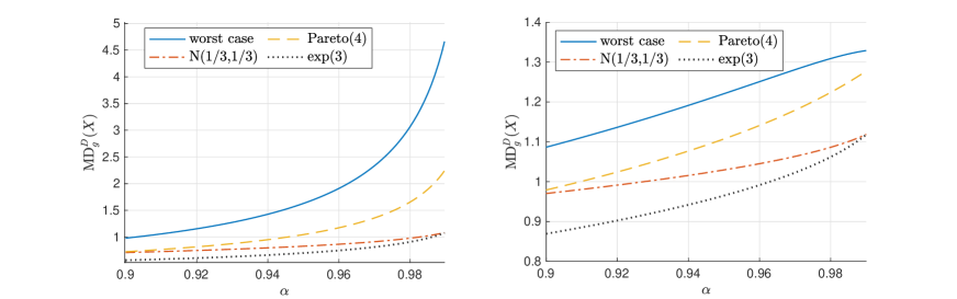
Figure 2: The values of of ${\mathrm{MD}}^{D}_{g}$ and $\overline{\mathrm{MD}}^{D}_{g}$ with $g(x)=x+e^{-x}-1$ (left) and $g(x)=1-e^{-x}$ (right)

Optimization problems under the uncertainty set of a Wasserstein ball are also common in the literature when quantifying the discrepancy between a benchmark distribution and alternative scenarios; see e.g., Esfahani and Kuhn (2018). For two distributions $F$ and $G$, the type-$p$ Wasserstein metric with $p\geqslant 1$, is given by

$$W_{p}(F,G)=\left(\int_{0}^{1}\left|F^{-1}(u)-G^{-1}(u)\right|^{p}\mathrm{\leavevmode\nobreak\ d}u\right)^{1/p}.$$

Denote by $\mathcal{M}_{p}$ the set of all distribution functions that have finite $p$th moment. For $F_{0}\in\mathcal{M}_{p}$ and $\varepsilon\geqslant 0$, we define the following uncertainty set based on the type-$p$ Wasserstein metric

$$\mathcal{B}_{p}(F_{0},\varepsilon)=\{F\in\mathcal{M}_{p}:W_{p}(F,F_{0})\leqslant\varepsilon\}.$$

The above uncertainty set is also known as a type-$p$ Wasserstein ball (see e.g., Kuhn et al. (2019) and Wu et al. (2022)), where $F_{0}$ is the center and $\varepsilon$ is the radius. Note that $\varepsilon=0$ corresponds to the case of no model uncertainty. In what follows, we focus on the type-$2$ Wasserstein ball. For any $\varepsilon\geqslant 0$, $g\in\mathcal{G}$ and $D\in\mathcal{D}^{p}$ with $p\in[1,2]$, we define the worst-case ${\mathrm{MD}}^{D}_{g}$ as

$$\widetilde{\mathrm{MD}}^{D}_{g}(X|\varepsilon)=\sup\left\{\mathrm{MD}^{D}_{g}(Y):F_{Y}\in\mathcal{B}_{2}(F_{X},\varepsilon)\right\}.$$

The following proposition gives a formula to compute the worst-case value of $\mathrm{MD}^{D}_{g}$ under the type-2 Wasserstein ball.

Proposition 5.

Suppose $p\in[1,2]$, $g\in\mathcal{G}$ and $D=D_{h}$ in (17) where $h\in\Phi^{p}$. We have

$$\widetilde{\mathrm{MD}}^{D}_{g}(X|\varepsilon)=\sup_{t\in[-1,1]}\left\{g\left(\varepsilon\sqrt{1-t^{2}}\left\|h^{\prime}\right\|_{2}+D(X)\right)+t\varepsilon+\mathbb{E}[X]\right\},{\leavevmode\nobreak\ \leavevmode\nobreak\ \leavevmode\nobreak\ \varepsilon\geqslant 0,\leavevmode\nobreak\ X\in L^{2}.}$$

Proof.

Denote by $\mathcal{M}=\{F_{Y}:Y\in L^{2},\leavevmode\nobreak\ \|Y-X\|_{2}\leqslant\varepsilon\}$. We first aim to show that $\mathcal{M}=\mathcal{B}_{2}(F_{X},\varepsilon)$. Note that $\mathcal{B}_{2}(F_{X},\varepsilon)=\{F_{Y}:Y\in L^{2},\leavevmode\nobreak\ \int_{0}^{1}|F_{Y}^{-1}(u)-F_{X}^{-1}(u)|^{2}\mathrm{d}u\leqslant\varepsilon^{2}\}$. It is obvious that $\mathcal{M}\subseteq\mathcal{B}_{2}(F_{X},\varepsilon)$ since $\|Y-X\|_{2}^{2}\geqslant\int_{0}^{1}|F_{Y}^{-1}(u)-F_{X}^{-1}(u)|^{2}\mathrm{d}u$ for any $X,Y\in L^{2}$. To see the converse direction, for any $F\in\mathcal{B}_{2}(F_{X},\varepsilon)$, let $Y\in L^{2}$ be such that $Y$ and $X$ are comonotonic and $Y$ has distribution $F$. It holds that $\|Y-X\|_{2}^{2}=\int_{0}^{1}|F^{-1}(u)-F_{X}^{-1}(u)|^{2}\mathrm{d}u\leqslant\varepsilon^{2}$, where the last step is due to $F\in\mathcal{B}_{2}(F_{X},\varepsilon)$. Hence, we have $F\in\mathcal{M}$. This implies that $\mathcal{B}_{2}(F_{X},\varepsilon)\subseteq\mathcal{M}$, and we have concluded that $\mathcal{M}=\mathcal{B}_{2}(F_{X},\varepsilon)$. Note that ${\rm MD}_{g}^{D}$ is law-invariant. We have

$$\widetilde{\mathrm{MD}}^{D}_{g}(X|\varepsilon) =\sup\{{\rm MD}_{g}^{D}(Y):F_{Y}\in\mathcal{B}_{2}(F_{X},\varepsilon)\}$$

$$=\sup_{\|Y-X\|_{2}\leqslant\varepsilon}{\rm MD}_{g}^{D}(Y)=\sup_{\|Y-X\|_{2}\leqslant\varepsilon}\left\{g(D(Y))+\mathbb{E}[Y]\right\}.$$ (21)

Denote by $\mu_{0}=\mathbb{E}[X]$. It holds that

$$\{\mathbb{E}[Y]:\|Y-X\|_{2}\leqslant\varepsilon\}=\{\mu_{0}+\mathbb{E}[V]:\|V\|_{2}\leqslant\varepsilon\}\subseteq[\mu_{0}-\varepsilon,\mu_{0}+\varepsilon].$$

Therefore, (6) reduces to

$$\sup_{\|Y-X\|_{2}\leqslant\varepsilon}\left\{g(D(Y))+\mathbb{E}[Y]\right\} =\sup_{\mu\in[\mu_{0}-\varepsilon,\mu_{0}+\varepsilon]}\leavevmode\nobreak\ \leavevmode\nobreak\ \leavevmode\nobreak\ \leavevmode\nobreak\ \sup_{\|Y-X\|_{2}\leqslant\varepsilon,\leavevmode\nobreak\ \mathbb{E}[Y]=\mu}\left\{g(D(Y))+\mathbb{E}[Y]\right\}$$

$$=\sup_{\mu\in[\mu_{0}-\varepsilon,\mu_{0}+\varepsilon]}\leavevmode\nobreak\ \leavevmode\nobreak\ \leavevmode\nobreak\ \leavevmode\nobreak\ \sup_{\|V\|_{2}\leqslant\varepsilon,\leavevmode\nobreak\ \mathbb{E}[V]=\mu-\mu_{0}}\left\{g(D(V+X))+\mu\right\}$$

$$=\sup_{\mu\in[\mu_{0}-\varepsilon,\mu_{0}+\varepsilon]}\leavevmode\nobreak\ \leavevmode\nobreak\ \leavevmode\nobreak\ \leavevmode\nobreak\ \sup_{\|V\|_{2}\leqslant\varepsilon,\leavevmode\nobreak\ \mathbb{E}[V]=\mu-\mu_{0}}\left\{g(D(V)+D(X))+\mu\right\}$$

$$=\sup_{\mu\in[\mu_{0}-\varepsilon,\mu_{0}+\varepsilon]}\leavevmode\nobreak\ \leavevmode\nobreak\ \leavevmode\nobreak\ \leavevmode\nobreak\ \sup_{\sigma^{2}(V)\leqslant\varepsilon^{2}-(\mu-\mu_{0})^{2},\leavevmode\nobreak\ \mathbb{E}[V]=\mu-\mu_{0}}\left\{g(D(V)+D(X))+\mu\right\},$$

where the third equality holds because $g$ is increasing and $D$ defined in (17) is subadditive and comonotonic additive, and we can construct $V$ and $X$ to be comonotonic. Since $g$ is increasing, the inner optimization problem is equivalent to maximizing $D(V)$ over $\{V:\sigma^{2}(V)\leqslant\varepsilon^{2}-(\mu-\mu_{0})^{2},\leavevmode\nobreak\ \mathbb{E}[V]=\mu-\mu_{0}\}$. Using the arguments in the proof of Proposition 4, we have

$$\sup\{D(V):\sigma^{2}(V)\leqslant\varepsilon^{2}-(\mu-\mu_{0})^{2},\leavevmode\nobreak\ \mathbb{E}[V]=\mu-\mu_{0}\}=\sqrt{\varepsilon^{2}-(\mu-\mu_{0})^{2}}\left\|h^{\prime}\right\|_{2}.$$

Therefore, we have

$$\widetilde{\mathrm{MD}}^{D}_{g}(X|\varepsilon) =\sup_{\mu\in[\mu_{0}-\varepsilon,\mu_{0}+\varepsilon]}\left\{g\left(\sqrt{\varepsilon^{2}-(\mu-\mu_{0})^{2}}\|h^{\prime}\|_{2}+D(X)\right)+\mu\right\}$$

$$=\sup_{t\in[-\varepsilon,\varepsilon]}\left\{g\left(\sqrt{\varepsilon^{2}-t^{2}}\left\|h^{\prime}\right\|_{2}+D(X)\right)+t+\mu_{0}\right\}$$

$$=\sup_{t\in[-1,1]}\left\{g\left(\varepsilon\sqrt{1-t^{2}}\left\|h^{\prime}\right\|_{2}+D(X)\right)+t\varepsilon+\mathbb{E}[X]\right\},$$

which completes the proof. ∎

In Proposition 5, our analysis is confined to the case of type-$2$ Wasserstein ball and signed Choquet integral $D_{h}$. Working with general deviation measure $D$ is not more difficult, as it only involves another supremum over $\Psi^{p}$ by using (16). For the general type-$p$ Wasserstein ball with $p\neq 2$, following similar arguments to those used in the proof of Proposition 5 leads us to

$$\sup\left\{\mathrm{MD}^{D}_{g}(Y):F_{Y}\in\mathcal{B}_{p}(F_{X},\varepsilon)\right\}=\sup_{\mu\in[\mathbb{E}[X]-\varepsilon,\mathbb{E}[X]+\varepsilon]}\leavevmode\nobreak\ \leavevmode\nobreak\ \leavevmode\nobreak\ \leavevmode\nobreak\ \sup_{\|V\|_{p}\leqslant\varepsilon,\leavevmode\nobreak\ \mathbb{E}[V]=\mu-\mathbb{E}[X]}\left\{g(D(V+X))+\mu\right\}.$$ (22)

We do not have an explicit formula to solve the inner supremum problem in the right-hand side of (22). This is due to the fact that $\|V\|_{p}$ and $\mathbb{E}[V]$ does not align very well unless $p=2$.

Example 6.

Let $g(x)=x-\log(1+x)$ for $x\in\mathbb{R}$ and $h(t)=(t-\alpha)_{+}/(1-\alpha)-t$ for $t\in[0,1]$ with $\alpha\in(0,1)$. We have $D:=D_{h}=\mathrm{ES}_{\alpha}-\mathbb{E}$, and it follows from Proposition 5 that

$$\widetilde{\mathrm{MD}}^{D}_{g}(X|\varepsilon)=\sup_{t\in[-1,1]}\left\{g\left(\varepsilon\sqrt{1-t^{2}}\sqrt{\frac{\alpha}{1-\alpha}}+\mathrm{ES}_{\alpha}(X)-\mathbb{E}[X]\right)+t\varepsilon+\mathbb{E}[X]\right\}$$

$$=\sup_{t\in[-1,1]}\left\{t\varepsilon+\varepsilon\sqrt{1-t^{2}}\sqrt{\frac{\alpha}{1-\alpha}}+\mathrm{ES}_{\alpha}(X)-\log\left(1+\varepsilon\sqrt{1-t^{2}}\sqrt{\frac{\alpha}{1-\alpha}}+\mathrm{ES}_{\alpha}(X)-\mathbb{E}[X]\right)\right\}.$$

Below we give another example of $D$. For $X\in L^{1}$, let $X_{1}$, $X_{2}$, $X$ be iid, and

$$D(X)=\mathrm{Gini}(X):=\frac{1}{2}\mathbb{E}\left[\left|X_{1}-X_{2}\right|\right].$$ (23)

The Gini deviation is a signed Choquet integral with a concave distortion function $h$ given by $h(t)=t-t^{2}$ for $t\in[0,1]$ (see e.g., Denneberg (1990)), i.e., $D={\rm Gini}=D_{h}$. By Proposition 5, we have

$$\widetilde{\mathrm{MD}}^{D}_{g}(X|\varepsilon) =\sup_{t\in[-1,1]}\left\{g\left(\frac{\sqrt{3}\varepsilon}{3}\sqrt{1-t^{2}}+\mathrm{Gini}(X)\right)+t\varepsilon+\mathbb{E}[X]\right\}$$

$$=\sup_{t\in[-1,1]}\left\{t\varepsilon+\mathbb{E}[X]+\frac{\sqrt{3}\varepsilon}{3}\sqrt{1-t^{2}}+\mathrm{Gini}(X)-\log\left(1+\frac{\sqrt{3}\varepsilon}{3}\sqrt{1-t^{2}}+\mathrm{Gini}(X)\right)\right\}.$$

The maximum values can be computed numerically. In Figure 3, by letting $g(x)=x-\log(1+x)$ and the benchmark distributions being normal, Pareto and exponential, we compute the worst values of $\mathrm{MD}^{D}_{g}(X)$ when $D=\mathrm{ES}_{\alpha}-\mathbb{E}$ with $\alpha=0.9$ and $D=\mathrm{Gini}$ for different values of uncertainty level $\varepsilon$.

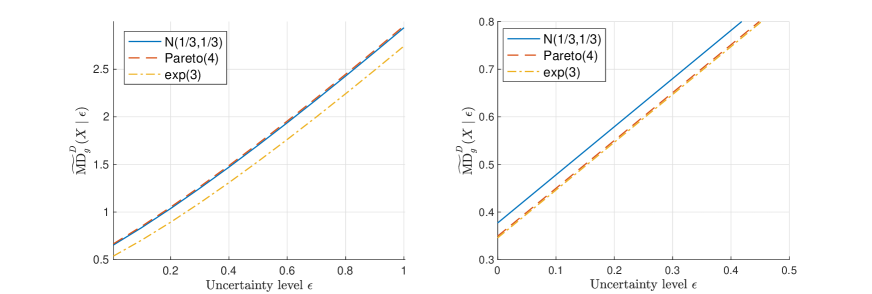
Figure 3: The values of $\widetilde{\mathrm{MD}}^{D}_{g}(X|\varepsilon)$ with $D=\mathrm{ES}_{\alpha}-\mathbb{E}$ (left) and $D=\mathrm{Gini}$ (right)

7 Non-parametric estimation

In this section, we consider the properties of non-parametric estimators of $\mathrm{MD}^{D}_{g}$ when $D$ is a convex signed Choquet integral; that is, $D$ is defined as $D_{h}$ in (17) with $h\in\mathcal{H}$.

The non-parametric estimators of $\mathrm{MD}^{D}_{g}(X)$ can be derived from those of $D_{h}$, VaR and the expectation, as we will explain in this section. For $p\in[1,\infty]$, suppose that $X_{1},X_{2},\ldots,X_{n}\in L^{p}$ are an iid sample from (the distribution of) a random variable $X$. Recall that the empirical distribution $\widehat{F}_{n}$ of $X_{1},\ldots,X_{n}$ is given by

$$\widehat{F}_{n}(x)=\frac{1}{n}\sum_{j=1}^{n}\mathds{1}_{\left\{X_{j}\leqslant x\right\}},\quad x\in\mathbb{R}.$$

Let $\widehat{\mathrm{MD}}^{D}_{g}(n)$ be the empirical estimator of $\mathrm{MD}^{D}_{g}(X)$, obtained by applying $\mathrm{MD}^{D}_{g}$ to the empirical distribution of $X_{1},\ldots,X_{n}$. We will establish consistency and asymptotic normality of the empirical estimators, based on corresponding results on empirical estimators of $\mathbb{E}[X]$ and $D_{h}(X)$. Let $\widehat{x}_{n}$ and $\widehat{D}_{h}(n)$ be the empirical estimators of $\mathbb{E}[X]$ and $D_{h}(X)$ based on the first $n$ sample data points. We make following standard regularity assumption on the distribution of the random variable $X$.

Assumption 1.

The distribution $F$ of $X\in\mathcal{X}$ is supported on a convex set and has a positive density function $f$ on the support. Denote by $\tilde{f}=f\circ F^{-1}$.

The proof of Theorem 5 below relies on standard techniques in empirical quantile processes, and it is given in Appendix C. In what follows, $g^{\prime}$ is the left derivative of $g$.

Theorem 5.

Fix $p\in[1,\infty)$. Let $g\in\mathcal{G}$ and $D=D_{h}$ where $h\in\Phi^{p}$. Suppose that $X_{1},\dots,X_{n}\in L^{p}$ are an iid sample from $X\in L^{p}$ and Assumption 1 holds. Then, $g(\widehat{D}(n))+\widehat{x}_{n}\stackrel{{\scriptstyle\mathbb{P}}}{{\rightarrow}}g\left(D(X)\right)+\mathbb{E}[X]$ as $n\to\infty$. Moreover, if $p<2$ and $X\in L^{\gamma}$ for some $\gamma>2p/(2-p)$, then we have

$$\sqrt{n}\left(\widehat{\mathrm{MD}}^{D}_{g}(n)-\mathrm{MD}^{D}_{g}(X)\right)\stackrel{{\scriptstyle\mathrm{d}}}{{\rightarrow}}\mathrm{N}\left(0,\sigma_{g}^{2}\right),$$

in which

$$\sigma^{2}_{g}=\int_{0}^{1}\int_{0}^{1}\frac{(h^{\prime}(1-s)g^{\prime}(D(X))+1)(h^{\prime}(1-t)g^{\prime}(D(X))+1)(s\wedge t-st)}{\tilde{f}(s)\tilde{f}(t)}\mathrm{d}t\mathrm{d}s.$$ (24)

The integrability conditions $h\in\Phi^{p}$ and $X\in L^{\gamma}$ with $\gamma>2p/(2-p)$, needed for asymptotic normality in Theorem 5, coincide with those in Jones and Zitikis (2003), who gave asymptotic normality of empirical estimators for distortion risk measures. In particular, in case $p=1$, we require $X\in L^{\gamma}$ with $\gamma>2$, which is a common assumption in weighted empirical quantile processes without distortion; see e.g., Shao and Yu (1996). The condition $p<2$ is also important. If $D_{h}\not\in\Phi^{2}$, then $D_{h}$ is not even finite on $L^{2}$, and we do not expect asymptotic normality in this case.

Note that the asymptotic variance $\sigma_{g}$ in (24) is decreasing in the left derivative $g^{\prime}$ of $g$. Therefore, if we replace $g$ by $\tilde{g}\in\mathcal{G}$ satisfying $\tilde{g}^{\prime}\leqslant g^{\prime}$, then the asymptotic variance, and thus the estimation error, will decrease. Note that a larger $g^{\prime}$ corresponds to a larger sensitivity to risk, as it measures how $\mathrm{MD}^{D}_{g}$ changes when $D(X)$ increases. Therefore, Theorem 5 gives a trade-off between risk sensitivity and statistical efficiency.

In what follows, we present some simulation results based on Theorem 5. We assume that $g(x)=x+e^{-x}-1$ and $g(x)=1-e^{-x}$, respectively. Simulation results are presented in the case of standard normal and Pareto risks with tail index 4. Let the sample size $n=10000$, and we repeat the procedure $5000$ times.

First, let $D=\mathrm{ES}_{\alpha}-\mathbb{E}$ with $\alpha=0.9$, then $\mathrm{MD}^{D}_{g}(X)$ is given as $\mathrm{MD}^{D}_{g}(X)=g(\mathrm{ES}_{\alpha}(X)-\mathbb{E}[X])+\mathbb{E}[X].$ In this case, we have $h^{\prime}(1-t)=\frac{1}{1-\alpha}\mathds{1}_{\{t\geqslant\alpha\}}-1$ and $\sigma^{2}_{g}$ in (24) can be computed explicitly. We compare the asymptotic variance of $\mathrm{MD}^{D}_{g}$ with that of $\mathrm{ES}_{\alpha}$, given by, via (24),

$$\begin{aligned} \sigma^{2}_{\mathrm{ES}}=\frac{1}{(1-\alpha)^{2}}\int_{\alpha}^{1}\int_{\alpha}^{1}\frac{s\wedge t-st}{\tilde{f}(s)\tilde{f}(t)}\mathrm{d}t\mathrm{d}s\end{aligned}.$$

In Figure 4 (a) and (b), the sample is simulated from standard normal risk. We can observe that, for $g(x)=x+e^{-x}-1$ and $D=\mathrm{ES}_{\alpha}-\mathbb{E}$, empirical estimates of $\mathrm{MD}^{D}_{g}$ match quiet well with the density function of $\mathrm{N}(0.93,2.85/n)$. In contrast, $\mathrm{ES}_{\alpha}$ empirical estimates match with the density function of $\mathrm{N}(1.76,3.71/n)$, whose asymptotic variance is larger than that of $\mathrm{MD}^{D}_{g}$. In Figure 4 (c) and (d), the sample is simulated from the Pareto distribution with tail index $4$. We can observe that $\mathrm{MD}^{D}_{g}(X)$ empirical estimates match quiet well with the density function of $\mathrm{N}(0.73,4.88/n)$ and ES empirical estimates match with the density function of $\mathrm{N}(1.37,10.19/n)$, whose asymptotic variance is also larger than the one of $\mathrm{MD}^{D}_{g}$. Since $g$ satisfies the 1-Lipschitz condition, the volatility of $D$ is reduced via the distortion by $g$.

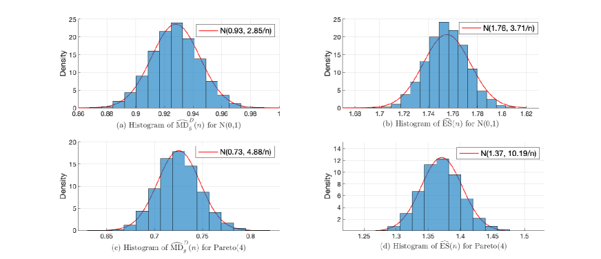
Figure 4: Left: $\widehat{\mathrm{MD}}^{D}_{g}(n)$ with $D=\mathrm{ES}_{\alpha}-\mathbb{E}$ and $g(x)=x+e^{-x}-1$; Right: $\widehat{\mathrm{ES}}_{\alpha}(n)$

In Figure 5 (a) and (b), for $g(x)=1-e^{-x}$ and $D=\mathrm{ES}_{\alpha}-\mathbb{E}$, we can observe that ${\mathrm{MD}}^{D}_{g}$ empirical estimates match quiet well with the density function of $\mathrm{N}(0.83,1.08/n)$ and $\mathrm{N}(0.98,1.97/n)$ when the samples are also simulated from the standard normal distribution or the Pareto distribution with tail index $4$. Also, the asymptotic variance are both smaller than those of ES empirical estimates.

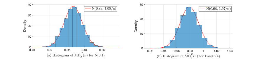
Figure 5: $\widehat{\mathrm{MD}}^{D}_{g}(n)$ with $D=\mathrm{ES}_{\alpha}-\mathbb{E}$ and $g(x)=1-e^{-x}$

If $g(x)=\lambda x$ with $\lambda\in(0,1)$, then we have $\mathrm{MD}^{D}_{g}(X)=\lambda\mathrm{ES}_{\alpha}(X)+(1-\lambda)\mathbb{E}[X]$. It is obvious that the asymptotic variance of $\mathbb{E}/\mathrm{ES}$-mixture is an increasing function with respect to $\lambda$ and thus is smaller than the one of $\mathrm{ES}$. Moreover, if $\lambda=1$, $\mathrm{MD}^{D}_{g}=\mathrm{ES}_{\alpha}$, and the values of $\sigma_{g}^{2}/n$ in Figure 6 (b) and (d) equal to those in Figure 4 (b) and (d).

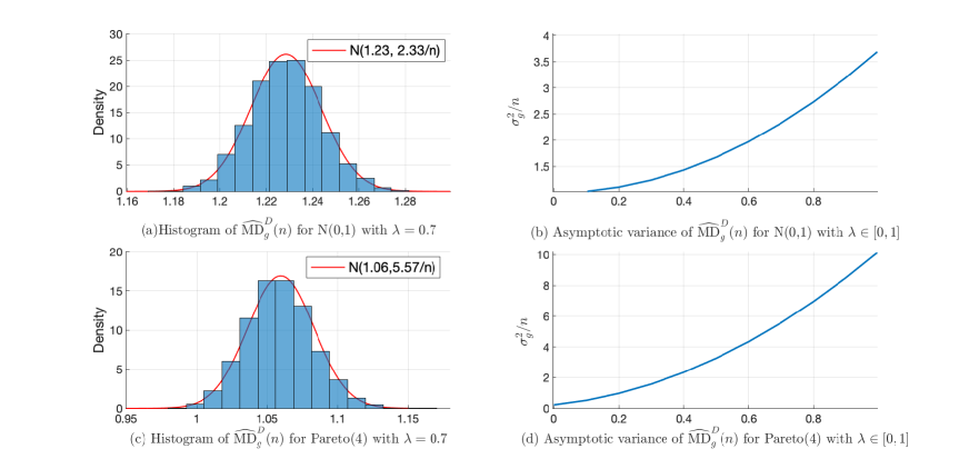
Figure 6: $\widehat{\mathrm{MD}}^{D}_{g}(n)$ with $D=\mathrm{ES}_{\alpha}-\mathbb{E}$ and $g(x)=\lambda x$

For another example, we assume that $D$ is the Gini deviation in (23). Then we have

$$\sigma^{2}_{g}=\int_{0}^{1}\int_{0}^{1}\frac{((2s-1)g^{\prime}(\mathrm{Gini}(X))+1)((2t-1)g^{\prime}(\mathrm{Gini}(X))+1)(s\wedge t-st)}{\tilde{f}(s)\tilde{f}(t)}\mathrm{d}t\mathrm{d}s.$$

Note that the asymptotic variance for $\mathrm{Gini}(X)+\mathbb{E}[X]$, denoted by $\sigma^{2}_{\mathrm{Gini}+\mathbb{E}}$, equals

$$\begin{aligned} \sigma^{2}_{\mathrm{Gini}+\mathbb{E}}=\int_{0}^{1}\int_{0}^{1}\frac{4ts(s\wedge t-st)}{\tilde{f}(s)\tilde{f}(t)}\mathrm{d}t\mathrm{d}s\end{aligned}.$$

Simulation results are presented in Figures 7 and 8 for $D=\rm{Gini}$ in the case of the standard normal distribution and the Pareto distribution with tail index 4, that also confirm the asymptotic normality of the empirical estimators in Theorem 5. Similarly, the asymptotic variance of $\mathbb{E}+\mathrm{Gini}$ is also larger than the one of ${\mathrm{MD}}_{g}^{D}$ based on $D=\rm Gini$.

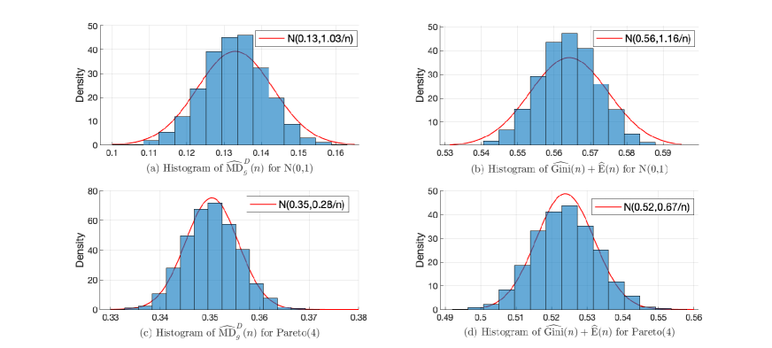
Figure 7: Left: $\widehat{\mathrm{MD}}^{D}_{g}(n)$ with $g(x)=x+e^{-x}-1$ and $D=\mathrm{Gini}$; Right: $\widehat{\mathrm{Gini}}(n)+\widehat{\mathbb{E}}(n)$

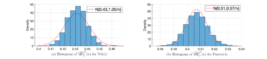
Figure 8: $\widehat{\mathrm{MD}}^{D}_{g}(n)$ with $D=\mathrm{Gini}$ and $g(x)=1-e^{-x}$

8 Conclusion

Even though mean-deviation measures are widely considered in the literature and have a lot of attractive features, there are few systemic treatments in the literature. In this paper, we studied the class $\mathrm{MD}^{D}_{g}$ of mean-deviation measures whose form is a combination of the deviation-related functional and the expectation, which enriches the axiomatic theory of risk measures. In particular, the obtained class always belongs to the class of consistent risk measures. We showed that $\mathrm{MD}^{D}_{g}$ can be coherent, convex or star-shaped risk measures, identified with the corresponding properties of the risk-weighting function $g$. By looking at this new class, the gap between convex risk measures and consistent risk measures, arguably opaque in the literature due to lack of explicit examples, becomes transparent. Moreover, two problems of model uncertainty based on $\mathrm{MD}^{D}_{g}$ were solved explicitly. Finally, the empirical estimators of $\mathrm{MD}^{D}_{g}$ can be formulated based on those of $D_{h}$, VaR and the expectation, and the asymptotic normality of the estimators is established. We find the asymptotic variance of $\mathrm{MD}^{D}_{g}$ is smaller than the one of risk measures without distortion; a useful feature in statistical estimation. This intuitively illustrates a trade-off between statistical efficiency and sensitivity to risk.

We discuss some future directions for the research of $\mathrm{MD}^{D}_{g}$. In fact, the form of $\mathrm{MD}^{D}_{g}$ (not necessarily monotonic) includes many commonly used reinsurance premium principle as special cases; see, e.g., the variance related principles (Furman and Landsman (2006) and Chi (2012)) and the Denneberg’s absolute deviation principle (Tan et al. (2020)). Thus, it would be interesting to formulate the optimal reinsurance problem where the reinsurance principle is computed by $\mathrm{MD}^{D}_{g}$. The optimal reinsurance strategies should rely on the properties and the form of $g$. It is also meaningful to consider risk sharing problems and portfolio selection problems under the criterion of minimizing $\mathrm{MD}^{D}_{g}$ under a similar framework to Grechuk et al. (2012, 2013) and Grechuk and Zabarankin (2012). Another direction of generalization is to relax cash-additivity we imposed throughout the paper to cash-subadditivity, as this allows for non-constant eligible assets when computing regulatory capital requirement; see El Karoui and Ravanelli (2009) and Farkas et al. (2014). Finally, we worked throughout with law-invariant mean-deviation measures with respect to a fixed probability measure. When the probability measure is uncertain, one needs to develop a framework of mean-deviation measures that can incorporate uncertainty and multiple scenarios in some forms (e.g., Cambou and Filipović (2017), Delage et al. (2019) and Fadina et al. (2023)).

Appendix A Monotonicity of mean-deviation models

In this appendix, we analyze monotonicity of mean-deviation models. Recall the necessary condition in Lemma 1, that is $\lambda D\in\overline{\mathcal{D}}^{p}$ for some $\lambda>0$. We aim to re-examine [M] of the mean-deviation model $U=V(\mathbb{E},D)$ and establish the characterization of [M] under this condition. We assume without loss of generality that $\lambda=1$, i.e., $D\in\overline{\mathcal{D}}^{p}$. For such $D$, by definition it is

$$\sup_{X\in{(L^{p})}^{\circ}}\frac{D(X)}{\mathrm{ess\mbox{-}sup}X-\mathbb{E}[X]}=1.$$ (25)

Proposition 6.

Fix $p\in[1,\infty]$. Let $D\in\overline{\mathcal{D}}^{p}$ and $U=V(\mathbb{E},D)$ be defined by (6) with $U(X)<\infty$ for all $X\in L^{p}$. Suppose that either $V:\mathbb{R}\times[0,\infty)$ is left continuous in its second argument or the maximizer in (25) is attainable. Then, $U$ satisfies [M] if and only if $V(m-a,d+a)\leqslant V(m,d)$ for all $m\in\mathbb{R}$ and $a,d\geqslant 0$.

Proof.

While the proof is similar to that of Proposition 4 in Grechuk et al. (2012), which establishes the same necessary and sufficient condition under the assumption that $U=V(\mathbb{E},D)$ is continuous, we provide the full details here for the sake of completeness and clarity.

We first verify sufficiency. For $X,Y\in L^{p}$ satisfying $X\leqslant Y$ and $X\neq Y$, we denote by $a=\mathbb{E}[Y]-\mathbb{E}[X]>0$, and it holds that $\mathrm{ess\mbox{-}sup}(X-Y)\leqslant 0$. By (25), we have

$$D(X-Y)\leqslant\mathrm{ess\mbox{-}sup}(X-Y)-\mathbb{E}[X-Y]\leqslant a.$$

Since $D$ satisfies (D4), we have

$$D(X)\leqslant D(Y)+D(X-Y)\leqslant D(Y)+a.$$ (26)

Therefore,

$$U(X) =V(\mathbb{E}[X],D(X))=V(\mathbb{E}[Y]-a,D(X))$$

$$\leqslant V(\mathbb{E}[Y],D(X)-a)\leqslant V(\mathbb{E}[Y],D(Y))=U(Y),$$

where the first inequality follows from the assumption by letting $m=\mathbb{E}[Y]$, $d=D(X)-a$, and the second inequality is due to $D(X)-a\leqslant D(Y)$ in (26). Hence, we conclude that $U$ satisfies [M]. Conversely, we first consider the case that $V$ is left continuous in its second argument. It follows from (25) that for any $\varepsilon>0$, there exists $X_{1}\in(L^{p})^{\circ}$ such that

$$1-\varepsilon\leqslant\frac{D(X_{1})}{\mathrm{ess\mbox{-}sup}X_{1}-\mathbb{E}[X_{1}]}\leqslant 1.$$

Let $m\in\mathbb{R}$ and $d,a\geqslant 0$. We define

$$X_{2}=a\frac{X_{1}-\mathrm{ess\mbox{-}sup}X_{1}}{\mathrm{ess\mbox{-}sup}X_{1}-\mathbb{E}[X_{1}]}\leavevmode\nobreak\ \leavevmode\nobreak\ {\rm and}\leavevmode\nobreak\ \leavevmode\nobreak\ X_{3}=\frac{d}{a}X_{2}+m+d.$$

Through standard calculation, $\mathbb{E}[X_{3}]=m$, $(1-\varepsilon)d\leqslant D(X_{3})\leqslant d$, $\mathbb{E}[X_{2}+X_{3}]=m-a$ and $(a+d)(1-\varepsilon)\leqslant D(X_{2}+X_{3})\leqslant a+d$. Note that $X_{2}\leqslant 0$ which implies $X_{2}+X_{3}\leqslant X_{3}$. Using [M], we have

$$V(m-a,(a+d)(1-\varepsilon))\leqslant V(\mathbb{E}[X_{2}+X_{3}],D(X_{2}+X_{3}))\leqslant V(\mathbb{E}[X_{3}],D(X_{3}))\leqslant V(m,d).$$

Letting $\varepsilon\downarrow 0$ and using the left continuity, we conclude that $V(m-a,a+d)\leqslant V(m,d)$ for for all $m\in\mathbb{R}$ and $a,d\geqslant 0$. Now, we assume that the maximizer in (25) is attainable, and the necessity follows a similar proof to the previous arguments by constructing $X_{1}$ such that $D(X_{1})/(\mathrm{ess\mbox{-}sup}X_{1}-\mathbb{E}[X_{1}])=1$. Hence, we complete the proof. ∎

We note that the ES-deviation $\mathrm{ES}_{\alpha}-\mathbb{E}$ for $\alpha\in(0,1)$ serves as an example where the maximizer in (25) is attainable.

Appendix B Axiomatization of monotonic mean-deviation measures

This appendix contains details on the axiomatization of monotonic mean-deviation measures, and its connection to the results of Grechuk et al. (2012). We first present two weaker axioms than A1 and A2, respectively.

• If $c_{1}\leqslant c_{2},$ then $c_{1}\succeq c_{2}$ for any $c_{1},c_{2}\in\mathbb{R}$.

• For any $X,Y$ satisfying $\mathbb{E}[X]=\mathbb{E}[Y]$ and $c>0$, $X\succeq Y$ if and only if $X+c\succeq Y+c$.

Grechuk et al. (2012) characterized a mean-deviation model $X\mapsto V(\mathbb{E}[X],D(X))$ using a set of axioms equivalent to A1, B2 and A3-A7. In contrast, to obtain the characterization in Theorem 2, we first use Axiom B1 to characterize $\mathrm{MD}^{D}_{g}$ in (8), where $g$ does not necessarily satisfy the 1-Lipschitz condition, and $D$ is not necessarily weakly upper-range dominated. The characterized $\mathrm{MD}^{D}_{g}$ contains more examples such as the mean-variance and the mean-SD functionals, which are not monotonic but satisfy the weak monotonicity.

Proposition 7.

Fix $p\in[1,\infty]$. A preference $\succeq$ satisfies Axioms B1 and A2–A7 if and only if $\succeq$ can be represented by $\mathrm{MD}^{D}_{g}=g\circ D+\mathbb{E}$ where $D\in\mathcal{D}^{p}$ is continuous and $g:[0,\infty)\rightarrow\mathbb{R}$ is continuous and strictly increasing.

Proof of Proposition 7.

We first show sufficiency. Let $\mathrm{MD}^{D}_{g}=g\circ D+\mathbb{E}$ represent $\succeq$ where $D\in\mathcal{D}^{p}$ and $g:[0,\infty)\rightarrow\mathbb{R}$ is some continuous, non-constant and increasing function. Axioms B1, A2, A3, A5 are straightforward by the properties of $D\in\mathcal{D}^{p}$.

The condition that $X\leqslant_{\rm cx}Y$ implies $X\succeq Y$ in Axiom A4 comes from Theorem 4.1 of Dana (2005) which showed that every law-invariant continuous convex measure on an atomless probability space is consistent with convex ordering. Moreover, for any $X\in(L^{p})^{\circ}$, since $D(X)>0$, together with the fact that $g$ is a strictly increasing function, we have $g(D(X))>g(0)$. Therefore, we have $\mathrm{MD}^{D}_{g}(X)>\mathrm{MD}^{D}_{g}(\mathbb{E}[X])$, which implies that $\mathbb{E}[X]\succ X$ for any $X\in(L^{p})^{\circ}$. Hence, we have verified Axiom A4.

To show Axiom A6 for $\mathrm{MD}^{D}_{g}$, for any $X,Y\in L^{p}$ such that $\mathbb{E}[X]=\mathbb{E}[Y]$ and $\mathrm{MD}^{D}_{g}(X)=\mathrm{MD}^{D}_{g}(Y)$, we have $g(D(X))=g(D(Y))$ and thus $D(X)=D(Y)$ because $g$ is strictly increasing. In this case, for any $\lambda>0$, we have

$$\mathrm{MD}^{D}_{g}(\lambda X+(1-\lambda)Y) =g(D(\lambda X+(1-\lambda)Y))+\lambda\mathbb{E}[X]+(1-\lambda)\mathbb{E}[Y]$$

$$\leqslant g(\lambda D(X)+(1-\lambda)D(Y))+\mathbb{E}[Y]$$

$$\leqslant g(D(X))+\mathbb{E}[X]=\mathrm{MD}^{D}_{g}(X).$$

Axiom A7 follows directly form the fact that $D$ and $g$ are continuous.

Next, we prove necessity. Axioms B1 and A2, A3 and A5 imply the existence of a unique certainty equivalence functional $\rho:L^{p}\rightarrow\mathbb{R}$, i.e., we have $X\succeq Y\Longleftrightarrow\rho(X)\leqslant\rho(Y)$ for any $X,Y\in L^{p}$, and $\rho(c)=c$ for any $c\in\mathbb{R}$; see Theorem 3.3 of Alcantud et al. (2003). In particular, $\rho$ is continuous by Axiom A7.

Let $X_{0}\in(L^{p})^{\circ}$ be such that $\mathbb{E}\left[X_{0}\right]=0$. Define $\phi(\lambda)=\rho\left(\lambda X_{0}\right)$ for $\lambda\geqslant 0$. We have $\phi(0)=\rho(0)$. The continuity of $\phi$ follows from the continuity of $\rho$. Since $\mathbb{E}[\lambda X_{0}]\succ\lambda X_{0}$ for any $\lambda>0$ by Axiom 5, we have $\rho(0)=\rho(\mathbb{E}[\lambda X_{0}])<\rho(\lambda X_{0})$. This implies that $\phi(\lambda)>\phi(0)$ for any $\lambda>0$. Moreover, it follows from Axiom 5 that $\rho(\lambda_{1}X_{0})\leqslant\rho(\lambda_{2}X_{0})$ for any $0<\lambda_{1}<\lambda_{2}$ as $\lambda_{1}X_{0}\leqslant_{\rm cx}\lambda_{2}X_{0}.$ Thus, we have $\phi(\lambda_{1})\leqslant\phi(\lambda_{2})$ which implies that $\phi$ is an increasing function on $[0,\infty)$. To show the inequality is strict, we assume by the contradiction, i.e., $\phi(\lambda_{1})=\phi(\lambda_{2})$. In this case, we have $\rho(\lambda_{1}X_{0})=\rho(\lambda_{2}X_{0})$ and $\rho(\lambda_{1}kX_{0})=\rho(\lambda_{2}kX_{0})$ for any $k>0$ by Axiom A3. Let $k=\lambda_{1}/\lambda_{2}<1$. By induction, we have $\rho(\lambda_{1}X_{0})=\rho(\lambda_{1}k^{n}X_{0})$ for any $n\in\mathbb{N}$. Letting $n\to\infty$, by Axiom A7, we have $\rho(\lambda_{1}X_{0})=\rho(0)$, which contradicts to Axiom A4. Thus, $\phi$ is a strictly increasing and continuous function on $[0,\infty)$, and its inverse function $\phi^{-1}(x):=\inf\{\lambda\in[0,\infty):\phi(\lambda)\geqslant x\}$ is also strictly increasing and continuous on the range of $\phi$.

For $X\in L^{p}$, let $\overline{X}=X-\mathbb{E}[X]$ and $D(X)=\phi^{-1}(\rho(\overline{X}))$. Since $\rho$ and $\phi$ are continuous functions, we know that $D$ is continuous. Next, we aim to verify that $D\in\mathcal{D}^{p}$. It is clear that $D$ is law-invariant since $\rho$ is law-invariant by Axiom A4, and thus (D5) holds. For any $c\in\mathbb{R}$, $D(X+c)=\phi^{-1}(\rho(\overline{X+c}))=D(X)$, which implies (D1). Note that Axiom A4 implies $\rho(\overline{X})>\rho(0)$ for all $X\in(L^{p})^{\circ}$. We have $D(X)=\phi^{-1}(\rho(\overline{X}))>\phi^{-1}(\rho(0))=0$ as $\phi^{-1}$ is strictly increasing. For any $c\in\mathbb{R}$, $D(c)=\phi^{-1}(\rho(0))=0$. Thus, (D2) holds. For any $X\in L^{p}$, we have

$$\rho(D(X)X_{0})=\phi(D(X))=\phi\circ\phi^{-1}(\rho(\overline{X}))=\rho(\overline{X})\Longleftrightarrow\overline{X}\simeq D(X)X_{0}.$$ (27)

It then follows from Axiom A3 that $\lambda\overline{X}\simeq\lambda D(X)X_{0}$ for all $\lambda\geqslant 0$. Hence, we have $\rho(\overline{\lambda X})=\rho(\lambda D(X)X_{0})$. On the other hand, $\overline{\lambda X}\simeq D(\lambda X)X_{0}$ implies $\rho(\overline{\lambda X})=\rho(D(\lambda X)X_{0})$. This concludes that $\rho(\lambda D(X)X_{0})=\rho(D(\lambda X)X_{0})$, which is equivalent to $\phi(\lambda D(X))=\phi(D(\lambda X))$. Note that $\phi$ is strictly increasing. It holds that $\lambda D(X)=D(\lambda X)$ which implies (D3). For $X,Y\in L^{p}$, if $X$ or $Y$ is constant, (D4) holds directly. Otherwise, we have $D(X)>0$ and $D(Y)>0$. Combining (27) and Axiom A3, we have $\rho(\overline{X}/D(X))=\rho(X_{0})$ and $\rho(\overline{Y}/D(Y))=\rho(X_{0})$ which implies $\rho(\overline{X}/D(X))=\rho(\overline{Y}/D(Y))$. Moreover, by Axiom A6, for all $\lambda\in[0,1]$,

$$\rho\left(\lambda\frac{\overline{X}}{D(X)}+(1-\lambda)\frac{\overline{Y}}{D(Y)}\right)\leqslant\rho\left(\frac{\overline{Y}}{D(Y)}\right)=\rho(X_{0}).$$

By setting $\lambda=D(X)/(D(X)+D(Y))$, we have $\rho\left(({\overline{X}+\overline{Y})}/{(D(X)+D(Y))}\right)\leqslant\rho(X_{0}).$ Applying (27) and Axiom A3 again, we have the following relation:

$$\frac{\overline{X}+\overline{Y}}{D(X)+D(Y)}=\frac{\overline{X+Y}}{D(X)+D(Y)}\simeq\frac{D(X+Y)X_{0}}{D(X)+D(Y)}.$$

Hence, denote by $k=D(X+Y)/(D(X)+D(Y))$, and we have $\rho\left(kX_{0}\right)\leqslant\rho(X_{0}),$ which implies $\phi\left(k\right)\leqslant\phi(1).$ Noting that $\phi$ is strictly increasing, we have $D(X+Y)\leqslant D(X)+D(Y)$ and (D4) holds.

For any $X\in L^{p}$, using $X\simeq\rho(X)$, we have $X-\mathbb{E}[X]\simeq\rho(X)-\mathbb{E}[X]$ by Axiom A2, which implies $\rho(X-\mathbb{E}[X])=\rho(X)-\mathbb{E}[X]$. Therefore, using (27),

$$\rho(X)=\rho(X-\mathbb{E}[X])+\mathbb{E}[X]=\rho(\overline{X})+\mathbb{E}[X]=\phi(D(X))+\mathbb{E}[X],\leavevmode\nobreak\ \leavevmode\nobreak\ \leavevmode\nobreak\ \mbox{for all $X\in L^{p}$},$$

where the last step follows from (27). This completes the proof. ∎

Proof of Theorem 2.

Sufficiency is straightforward by combining Theorem 1, Lemma 1 and Proposition 7. Next, we show the necessity. By Proposition 7, $\succeq$ can be represented by $\mathrm{MD}^{D^{\prime}}_{f}=f\circ D^{\prime}+\mathbb{E}$ where $D^{\prime}\in\mathcal{D}^{p}$, and $f:[0,\infty)\rightarrow\mathbb{R}$ is some continuous and strictly increasing function. Since $\mathrm{MD}^{D^{\prime}}_{f}$ satisfies monotonicity, by Lemma 1, we have $D^{\prime}\in\overline{\mathcal{D}}^{p}_{K}$. Define $g=f\circ D$ and $D=D^{\prime}/K$, we have $\mathrm{MD}^{D^{\prime}}_{f}=\mathrm{MD}^{D}_{g}=g\circ D+\mathbb{E}$ where $g:[0,\infty)\rightarrow\mathbb{R}$ is some continuous and strictly increasing function and $D\in\mathcal{\overline{D}}^{p}$. By Theorem 1, $g$ is 1-Lipschitz. Hence, we complete the proof. ∎

Appendix C Proof of Theorem 5

This appendix contains the proof of Theorem 5.

Proof.

The Law of Large Numbers yields $\widehat{x}_{n}\stackrel{{\scriptstyle\mathbb{P}}}{{\rightarrow}}\mathbb{E}[X]$. By Theorem 2.6 of Krätschmer et al. (2014), the empirical estimator for a finite convex risk measure on $L^{p}$ is consistent, that is, $\widehat{D}(n)+\widehat{x}_{n}\stackrel{{\scriptstyle\mathbb{P}}}{{\rightarrow}}D(X)+\mathbb{E}[X]$, and this gives $\widehat{D}(n)\stackrel{{\scriptstyle\mathbb{P}}}{{\rightarrow}}D(X)$. Moreover, since $g\in\mathcal{G}$, we have $g(\widehat{D}(n))+\widehat{\mathbb{E}}[n]\stackrel{{\scriptstyle\mathbb{P}}}{{\rightarrow}}g(D(X))+\mathbb{E}[X]$. This proves the first part of the result.

Next, we will show the asymptotic normality. Let $B=(B_{t})_{t\in[0,1]}$ be a standard Brownian bridge, and let $d_{n}=\sqrt{n}(\widehat{D}(n)-D(X))$, $e_{n}=\sqrt{n}(\widehat{x}_{n}-\mathbb{E}[X])$, and $g_{n}=\sqrt{n}(g(\widehat{D}(n))-g(D(X)))$. We need to first show

$$(d_{n},e_{n})\stackrel{{\scriptstyle\mathrm{d}}}{{\rightarrow}}(Z,W):=\left(\int_{0}^{1}\frac{B_{s}h^{\prime}(1-s)}{\tilde{f}(s)}\mathrm{d}s,\int_{0}^{1}\frac{B_{s}}{\tilde{f}(s)}\mathrm{d}s\right).$$ (28)

By the Cramér-Wold theorem, it suffices to show

$$ad_{n}+be_{n}\stackrel{{\scriptstyle\mathrm{d}}}{{\rightarrow}}aZ+bW\mbox{\leavevmode\nobreak\ for all $a,b\in\mathbb{R}$.}$$ (29)

Note that $aD+b\mathbb{E}$ can be written as an integral of the quantile, that is,

$$aD(X)+b\mathbb{E}[X]=\int_{0}^{1}F^{-1}(t)(ah^{\prime}(1-t)+b)\mathrm{d}t.$$

Denote by $A_{n}$ the empirical quantile process, that is,

$$A_{n}(t)=\sqrt{n}(\widehat{F}^{-1}_{n}(t)-F^{-1}(t)),\leavevmode\nobreak\ \leavevmode\nobreak\ \leavevmode\nobreak\ t\in(0,1).$$

It follows that

$$ad_{n}+be_{n}=\int_{0}^{1}A_{n}(t)(ah^{\prime}(1-t)+b)\mathrm{d}t.$$

Using this representation, the convergence (29) can be verified using Theorem 3.2 of Jones and Zitikis (2003), and we briefly verify it here. It is well known that, under Assumption 1, as $n\to\infty$, $A_{n}$ converges to the Gaussian process $B/\tilde{f}$ in $L^{\infty}[1-\delta,1+\delta]$ for any $\delta>0$ (see e.g., Del Barrio et al. (2005)). This yields

$$\int_{\delta}^{1-\delta}A_{n}(t)(ah^{\prime}(1-t)+b)\mathrm{d}t\stackrel{{\scriptstyle\mathrm{d}}}{{\rightarrow}}\int_{\delta}^{1-\delta}\frac{B_{t}}{\tilde{f}(t)}(ah^{\prime}(1-t)+b)\mathrm{d}t.$$

To show (29), it suffices to verify

$$\int_{\delta}^{1-\delta}\frac{B_{t}}{\tilde{f}(t)}(ah^{\prime}(1-t)+b)\mathrm{d}t\to\int_{0}^{1}\frac{B_{t}}{\tilde{f}(t)}(ah^{\prime}(1-t)+b)\mathrm{d}t\mbox{\leavevmode\nobreak\ \leavevmode\nobreak\ \leavevmode\nobreak\ as $\delta\downarrow 0$}.$$ (30)

Denote by $w_{t}=t(1-t)$. Since $h\in\Phi^{p}$ and $X\in L^{\gamma}$, we have, for some $C>0$,

$$|h^{\prime}(1-t)|\leqslant Cw_{t}^{1/p-1};\leavevmode\nobreak\ \leavevmode\nobreak\ \leavevmode\nobreak\ |F^{-1}(t)|\leqslant Cw_{t}^{-1/\gamma};\leavevmode\nobreak\ \leavevmode\nobreak\ \leavevmode\nobreak\ \frac{1}{\tilde{f}(t)}=\frac{\mathrm{d}F^{-1}(t)}{\mathrm{d}t}\leqslant Cw_{t}^{-1/\gamma-1}.$$

Note that $1/p-1/\gamma>1/2$ and $B_{t}=o_{\mathbb{P}}(w_{t}^{1/2-\varepsilon})$ for any $\varepsilon>0$ as $t\to 0$ or $1$. Hence, for some $\eta>0$,

$$\left|B_{t}\frac{ah^{\prime}(1-t)+b}{\tilde{f}(t)}\right|=o_{\mathbb{P}}(w_{t}^{\eta-1})\mbox{\leavevmode\nobreak\ \leavevmode\nobreak\ \leavevmode\nobreak\ for $t\in(0,1)$},$$

and this guarantees (30). Therefore, (28) holds.

By the Mean Value Theorem, there exists $x_{0}$ between $D(X)$ and $\widehat{D}(n)$ such that

$$\sqrt{n}(g(\widehat{D}(n))-g(D(X)))=g^{\prime}(x_{0})\sqrt{n}(\widehat{D}(n)-D(X)).$$

Using the fact that $\widehat{D}(n)\to D(X)$, we get

$$(g_{n},e_{n})\stackrel{{\scriptstyle\mathrm{d}}}{{\rightarrow}}\left(g^{\prime}(D(X))\int_{0}^{1}\frac{B_{s}h^{\prime}(1-s)}{\tilde{f}(s)}\mathrm{d}s,\int_{0}^{1}\frac{B_{s}}{\tilde{f}(s)}\mathrm{d}s\right).$$

Hence,

$$\sqrt{n}\left(\widehat{\mathrm{MD}}^{D}_{g}(n)-\mathrm{MD}^{D}_{g}(X)\right)=g_{n}+e_{n}\stackrel{{\scriptstyle\mathrm{d}}}{{\rightarrow}}g^{\prime}(D(X))\int_{0}^{1}\frac{B_{s}h^{\prime}(1-s)}{\tilde{f}(s)}\mathrm{d}s+\int_{0}^{1}\frac{B_{s}}{\tilde{f}(s)}\mathrm{d}s,$$

or equivalently,

$$\sqrt{n}\left(\widehat{\mathrm{MD}}^{D}_{g}(n)-\mathrm{MD}^{D}_{g}(X)\right)\stackrel{{\scriptstyle\mathrm{d}}}{{\rightarrow}}\int_{0}^{1}\frac{B_{s}}{\tilde{f}(s)}(h^{\prime}(1-s)g^{\prime}(D(X))+1)\mathrm{d}s.$$

Using the convariance property of the Brownian bridge, that is, $\mathrm{Cov}(B_{t},B_{s})=s-st$ for $s<t$, we have

$$\mathrm{Var}\left[\int_{0}^{1}\frac{B_{s}(h^{\prime}(1-s)g^{\prime}(D(X))+1)}{\tilde{f}(s)}\mathrm{d}s\right]$$

$$=\mathbb{E}\left[\int_{0}^{1}\int_{0}^{1}\frac{(h^{\prime}(1-s)g^{\prime}(D(X))+1)(h^{\prime}(1-t)g^{\prime}(D(X))+1)B_{s}B_{t}}{\tilde{f}(s)\tilde{f}(t)}\mathrm{d}t\mathrm{d}s\right]$$

$$=\int_{0}^{1}\int_{0}^{1}\frac{(h^{\prime}(1-s)g^{\prime}(D(X))+1)(h^{\prime}(1-t)g^{\prime}(D(X))+1)(s\wedge t-st)}{\tilde{f}(s)\tilde{f}(t)}\mathrm{d}t\mathrm{d}s.$$

Thus, $\sqrt{n}\left(\widehat{\mathrm{MD}}^{D}_{g}(n)-\mathrm{MD}^{D}_{g}(X)\right)\stackrel{{\scriptstyle\mathrm{d}}}{{\rightarrow}}\mathrm{N}(0,\sigma^{2}_{g})$ in which $\sigma^{2}_{g}$ is given by (24). ∎

References

- Alcantud et al. (2003) Alcantud, J. C. R. and Bosi, G. (2003). On the existence of certainty equivalents of various relevant types. Journal of Applied Mathematics, 2003(9), 447–458.
- Artzner et al. (1999) Artzner, P., Delbaen, F., Eber, J.-M. and Heath, D. (1999). Coherent measures of risk. Mathematical Finance, 9(3), 203–228.
- Bellini et al. (2022) Bellini, F., Fadina, T., Wang, R. and Wei, Y. (2022). Parametric measures of variability induced by risk measures. Insurance: Mathematics and Economics, 106, 270–284.
- Bellini et al. (2014) Bellini, F., Klar, B., Müeller, A. and Gianin, E. R. (2014). Generalized quantiles as risk measures. Insurance: Mathematics and Economics, 54, 41–48.
- Burzoni et al. (2022) Burzoni, M., Munari, C. and Wang, R. (2022). Adjusted expected shortfall. Journal of Banking and Finance, 134, 106297.
- Castagnoli et al. (2022) Castagnoli, E., Cattelan, G., Maccheroni, F., Tebaldi, C. and Wang, R. (2022). Star-shaped risk measures. Operations Research, 70(5), 2637–2654.
- Chi (2012) Chi, Y. (2012). Optimal reinsurance under variance related premium principles. Insurance: Mathematics and Economics, 51(2), 310–321.
- Cambou and Filipović (2017) Cambou, M. and Filipović, D. (2017). Model uncertainty and scenario aggregation. Mathematical Finance, 27(2), 534–567.
- Dana (2005) Dana R. A. (2005). A representation result for concave Schur-concave functions. Mathematical Finance, 15(4), 613–634.
- Del Barrio et al. (2005) Del Barrio, E., Giné, E. and Utzet, F. (2005). Asymptotics for functionals of the empirical quantile process, with applications to tests of fit based on weighted Wasserstein distances. Bernoulli, 11(1), 131–189.
- Delage et al. (2019) Delage, E., Kuhn, D. and Wiesemann, W. (2019). “Dice”-sion-making under uncertainty: When can a random decision reduce risk? Management Science, 65(7), 3282–3301.
- Denneberg (1990) Denneberg, D. (1990). Premium calculation: Why standard deviation should be replaced by absolute deviation. ASTIN Bulletin, 20, 181–190.
- Dhaene et al. (2006) Dhaene, J., Vanduffel, S., Goovaerts, M. J., Kaas, R., Tang, Q. and Vyncke, D. (2006). Risk measures and comonotonicity: A review. Stochastic Models, 22(4), 573–606.
- Drapeau and Kupper (2013) Drapeau, S. and Kupper, M. (2013). Risk preferences and their robust representation. Mathematics of Operations Research, 38(1), 28–62.
- El Karoui and Ravanelli (2009) El Karoui, N. and Ravanelli, C. (2009). Cash subadditive risk measures and interest rate ambiguity. Mathematical Finance, 19(4), 562–590.
- Esfahani and Kuhn (2018) Esfahani, P. M. and Kuhn, D. (2018). Data-driven distributionally robust optimization using the Wasserstein metric: Performance guarantees and tractable reformulations. Mathematical Programming, 171(1-2), 115–166.
- Fadina et al. (2023) Fadina, T., Liu, Y. and Wang, R. (2023). A framework for measures of risk under uncertainty. Finance and Stochastics, forthcoming.
- Fan (1953) Fan, K. (1953). Minimax theorems. Proceedings of the National Academy of Sciences, 39(1), 42–47.
- Farkas et al. (2014) Farkas, W., Koch-Medina, P. and Munari, C. (2014). Beyond cash-additive risk measures: When changing the numeraire fails. Finance and Stochastics, 18, 145–173.
- Filipović and Svindland (2008) Filipović, D. and Svindland, G. (2008). Optimal capital and risk allocations for law- and cash-invariant convex functions. Finance and Stochastics, 12, 423–439.
- Föllmer and Schied (2002) Föllmer, H. and Schied, A. (2002). Convex measures of risk and trading constraints. Finance and Stochastics, 6, 429–447.
- Föllmer and Schied (2016) Föllmer, H. and Schied, A. (2016). Stochastic Finance. An Introduction in Discrete Time. Fourth Edition. Walter de Gruyter, Berlin.
- Frittelli and Rosazza Gianin (2002) Frittelli, M. and Rosazza Gianin, E. (2002). Putting order in risk measures. Journal of Banking and Finance, 26,1473–1486.
- Furman and Landsman (2006) Furman, E. and Landsman, Z. (2006). Tail variance premium with applications for elliptical portfolio of risks. ASTIN Bulletin, 36, 433–462.
- Grechuk et al. (2012) Grechuk, B., Molyboha, A. and Zabarankin, M. (2012). Mean‐deviation analysis in the theory of choice. Risk Analysis, 32(8), 1277–1292.
- Grechuk et al. (2013) Grechuk, B., Molyboha, A. and Zabarankin, M. (2013). Cooperative games with general deviation measures. Mathematical Finance, 23(2), 339–365.
- Grechuk and Zabarankin (2012) Grechuk, B. and Zabarankin, M. (2012). Optimal risk sharing with general deviation measures. Annals of Operations Research, 200(1), 9–21.
- Han et al. (2023) Han, X., Wang, B., Wang, R. and Wu, Q. (2023). Risk concentration and the mean-Expected Shortfall criterion. Mathematical Finance, forthcoming.
- Herdegen and Khan (2022a) Herdegen, M. and Khan, N. (2022a). Mean- portfolio selection and -arbitrage for coherent risk measures. Mathematical Finance, 32(1), 226–272.
- Herdegen and Khan (2022b) Herdegen, M. and Khan, N. (2022b). Sensitivity to large losses and -arbitrage for convex risk measures. arXiv: 2202.07610.
- Jones and Zitikis (2003) Jones, B. L. and Zitikis, R. (2003). Empirical estimation of risk measures and related quantities. North American Actuarial Journal, 7(4), 44–54.
- Kaina and Rüschendorf (2009) Kaina, M. and Rüschendorf, L. (2009). On convex risk measures on -spaces. Mathematical Methods of Operations Research, 69, 475–495.
- Krätschmer et al. (2014) Krätschmer, V., Schied, A. and Zähle, H. (2014). Comparative and qualitative robustness for law-invariant risk measures. Finance and Stochastics, 18(2), 271–295.
- Kuhn et al. (2019) Kuhn, D., Esfahani, P. M., Nguyen, V. A. and Shafieezadeh-Abadeh, S. (2019). Wasserstein distributionally robust optimization: theory and applications in machine learning. INFORMS TutORials in Operations Research, 130–166.
- Laeven and Stadje (2013) Laeven, R. J. and Stadje, M. (2013). Entropy coherent and entropy convex measures of risk. Mathematics of Operations Research, 38(2), 265–293.
- Liu et al. (2020) Liu, F., Cai, J., Lemieux, C. and Wang, R. (2020). Convex risk functionals: Representation and applications. Insurance: Mathematics and Economics, 90, 66–79.
- Maccheroni et al. (2009) Maccheroni, F., Marinacci, M., Rustichini, A. and Taboga, M. (2009). Portfolio selection with monotone mean‐variance preferences. Mathematical Finance, 19(3), 487–521.
- Mao and Wang (2020) Mao, T. and Wang, R. (2020). Risk aversion in regulatory capital calculation. SIAM Journal on Financial Mathematics, 11(1), 169–200.
- Markowitz (1952) Markowitz, H. (1952). Portfolio selection. Journal of Finance, 7(1), 77–91.
- McNeil et al. (2015) McNeil, A. J., Frey, R. and Embrechts, P. (2015). Quantitative Risk Management: Concepts, Techniques and Tools. Revised Edition. Princeton, NJ: Princeton University Press.
- Newey and Powell (1987) Newey, W. and Powell, J. (1987). Asymmetric least squares estimation and testing. Econometrica, 55(4), 819–847.
- Pesenti et al. (2020) Pesenti, S., Wang, Q. and Wang R. (2020). Optimizing distortion risk metrics with distributional uncertainty. arXiv: 2011.04889.
- Rockafellar and Uryasev (2013) Rockafellar, R. T. and Uryasev, S. (2013). The fundamental risk quadrangle in risk management, optimization and statistical estimation. Surveys in Operations Research and Management Science, 18(1–2), 33–53.
- Rockafellar et al. (2006) Rockafellar, R. T., Uryasev, S. and Zabarankin, M. (2006). Generalized deviations in risk analysis. Finance and Stochastics, 10(1), 51–74.
- Rothschild and Stiglitz (1970) Rothschild, M. and Stiglitz, J. (1970). Increasing risk I. A definition. Journal of Economic Theory, 2(3), 225–243.
- Shaked and Shanthikumar (2007) Shaked, M. and Shanthikumar, J.G. (2007). Stochastic Orders. Springer Series in Statistics.
- Shao and Yu (1996) Shao, Q. M. and Yu, H. (1996). Weak convergence for weighted empirical processes of dependent sequences. Annals of Probability, 2098–2127.
- Sharpe (1964) Sharpe, (1964). Capital Asset Prices: A Theory of Market Equilibrium under Conditions of Risk. Journal of Finance, 19(3), 425–442.
- Simaan (1997) Simaan, Y. (1997). Estimation risk in portfolio selection: the mean variance model versus the mean absolute deviation model. Management Science, 43(10), 1437–1446.
- Tan et al. (2020) Tan, K. S., Wei, P., Wei, W., and Zhuang, S. C. (2020). Optimal dynamic reinsurance policies under a generalized Denneberg’s absolute deviation principle. European Journal of Operational Research, 282(1), 345–362.
- Wang et al. (2020a) Wang, Q., Wang, R. and Wei, Y. (2020a). Distortion riskmetrics on general spaces. ASTIN Bulletin, 50(3), 827–851.
- Wang et al. (2015) Wang, R., Bignozzi, V. and Tsakanas, A. (2015). How superadditive can a risk measure be? SIAM Jounral on Financial Mathematics, 6, 776–803.
- Wang et al. (2020b) Wang, R., Wei, Y. and Willmot, G. E. (2020b). Characterization, robustness, and aggregation of signed Choquet integrals. Mathematics of Operations Research, 45(3), 993–1015.
- Wang and Zitikis (2021) Wang, R. and Zitikis, R. (2021). An axiomatic foundation for the Expected Shortfall. Management Science, 67, 1413–1429.
- Williamson (1956) Williamson, R. E. (1956). Multiply monotone functions and their Laplace transforms. Duke Mathematical Journal, 23(2), 189–207.
- Wu et al. (2022) Wu, Q., Li, J. Y. M. and Mao, T. (2022). On generalization and regularization via Wasserstein distributionally robust optimization. arXiv:2212.05716.
- Yaari (1987) Yaari, M. E. (1987). The dual theory of choice under risk. Econometrica, 55(1), 95–115.