Data-Driven Autoencoder Numerical Solver with Uncertainty Quantification for Fast Physical Simulations

Abstract

Traditional partial differential equation (PDE) solvers can be computationally expensive, which motivates the development of faster methods, such as reduced-order-models (ROMs). We present GPLaSDI, a hybrid deep-learning and Bayesian ROM. GPLaSDI trains an autoencoder on full-order-model (FOM) data and simultaneously learns simpler equations governing the latent space. These equations are interpolated with Gaussian Processes, allowing for uncertainty quantification and active learning, even with limited access to the FOM solver. Our framework is able to achieve up to 100,000 times speed-up and less than 7$\%$ relative error on fluid mechanics problems.

1 Introduction

Over the last few decades, advances in numerical simulation methods and cheaper computational power have expanded the use of simulation across various fields, such as engineering design, digital twins, and decision making with application including aerospace, automotive, electronics and physics [16, 7, 2, 10]. Traditional numerical simulations often rely on high-fidelity solvers, which are generally accurate, but expensive [21, 26, 3]. This has historically motivated the development of reduced-order-models (ROM) which, at the cost of a drop in accuracy, can be much faster than high-fidelity full-order models (FOM).

Many ROM methods rely on projecting FOM data into a lower dimensional space, where the physical system’s governing equations are simpler to solve numerically [4, 22, 24]. Linear projection methods have been used with great success, but they often struggle with advection-dominated fluid flow problems [17, 11]. Thus, in recent years, non-linear approaches, using for instance neural networks, have gained significant popularity [20, 14, 19]. In their work, Champion et. al. [8] proposed a framework to identify governing dynamical systems in latent space of autoencoders. These identified governing sets of ordinary differential equations (ODEs), learned using SINDy algorithms [6, 23, 9, 5, 25], can be used to described the training data dynamics in a much simpler way. This work has been subsequently extended to reduced-order-modelling by Fries et. al., in a framework known as Latent Space Dynamics Identification (LaSDI) [11].

In LaSDI, an autoencoder is trained on FOM data, and the set of ODEs governing the latent space for each corresponding FOM datapoint is identified using SINDy. The ODE coefficients can then be interpolated with respect to the FOM parameters, and used to predict sets of ODEs associated with any new test parameters. ROM predictions can then easily be made by integrating the ODEs numerically and feeding the dynamics into the decoder. This work was later extended in greedy-Latent Space Dynamics Identification (gLaSDI) [13] by introducing an active learning framework and a joint training of the autoencoder and the latent space ODEs. During the training, additional data is added by feeding the model’s prediction into the PDE residual. The simulation parameter yielding the largest residual error is picked as a sampling point, for which a new FOM run is performed and the resulting data added to the training set. This strategy allows for collecting data where it is the most needed, while minimizing the number of FOM runs.

While robust and accurate, gLaSDI requires to have access to the PDE residual for sampling new data (intrusive ROM). This can be cumbersome and expensive to evaluate, especially when dealing with multi-scale and/or multi-physics problems, and sophisticated numerical solvers. In this paper, we introduced Gaussian Process Latent Space Dynamics Identification (GPLaSDI), a new LaSDI framework with non-intrusive greedy sampling (no residual evaluation required). We propose to use Gaussian Processes (GP) to interpolate the sets of ODE coefficients, instead of deterministic methods like in LaSDI and gLaSDI [11, 13]. This allows, for new test parameters, to propagate the uncertainty over the ODE coefficients to the latent space dynamics, and then to the decoder output. Our approach has two major advantages: first, we can quantify the uncertainty over ROM predictions. Second, we can use that uncertainty to pick new FOM sampling datapoints, without relying on the PDE residual.

2 Gaussian Process Latent Space Dynamics Identification

We consider physical systems described by time-dependant PDEs of the following form:

$$\frac{\partial\mathbf{u}}{\partial t}=\mathbf{f}(\mathbf{u},t,x\,|\,\boldsymbol{\mu})\hskip 25.29494pt(t,x)\in[0,t_{\text{max}}]\times\Omega\hskip 25.29494pt\mathbf{u}(t=0,x\,|\,\boldsymbol{\mu})=\mathbf{u_{0}}(x\,|\,\boldsymbol{\mu})$$ (1)

The vector of physical quantities u is defined over a time interval $[0,t_{\text{max}}]$ and spatial domain $\Omega$. The PDE and its initial condition $\textbf{u}_{0}$ are parameterized by a parameter vector $\boldsymbol{\mu}\in\mathcal{D}$. We assume that equation 1 can be solved with a high-fidelity FOM simulation, and we denote $\mathbf{U}^{(i)}=[\mathbf{u}_{0}^{(i)},\dots,\mathbf{u}_{N_{t}}^{(i)}]^{\top}\in\mathbb{R}^{(N_{t}+1)\times N_{u}}$ the matrix representing a numerical solution for parameter $\boldsymbol{\mu}^{(i)}\in\mathcal{D}$, computed over $N_{t}$ time steps and $N_{u}$ spatial nodes. The collection of $N_{\mu}$ FOM data points is written $\mathbf{U}=[\mathbf{U}^{(1)},\dots,\mathbf{U}^{(N_{\mu})}]$

We train an autoencoder on $\mathbf{U}$, and denote $\mathbf{Z}=\phi_{e}(\mathbf{U}|\mathbf{\theta}_{\text{enc}})\in\mathbb{R}^{N_{\mu}\times(N_{t}+1)\times N_{z}}$ the encoder output. $N_{z}$ is the latent space dimension, chosen arbitrarily (but such that $N_{z}\ll N_{u}$). The decoder output is $\mathbf{\hat{U}}=\phi_{d}(\mathbf{Z}|\mathbf{\theta}_{\text{dec}})$, and the training reconstruction loss is a standard mean-squared-error, $\mathcal{L}_{AE}(\mathbf{\theta}_{\text{enc}},\mathbf{\theta}_{\text{dec}})=|\!|\mathbf{U}-\mathbf{\hat{U}}|\!|_{2}^{2}$.

The architecture of the autoencoder is chosen such that the time dimension is unchanged. As a result, the latent space can be interpreted as a dynamical system, described by $N_{z}$ abstract variables. Hence, the encoder effectively transforms data described by a PDE into data described by an (unknown) system of ODEs, written as:

$$\mathbf{\dot{Z}}^{(i)}=\psi_{DI}(\mathbf{Z}^{(i)}|\boldsymbol{\mu}^{(i)})$$ (2)

$\mathbf{\dot{Z}}^{(i)}$ refers to the time derivative of the set of latent space variables for data point $i\in[\![1,N_{\mu}]\!]$. For each training parameters $\boldsymbol{\mu}^{(i)}$, we use an algorithm known as SINDy (Sparse Identification of Non-Linear Dynamics) [6] to learn a suitable set of explicit governing ODEs. The key idea of SINDy is to approximate $\psi_{DI}$ as a linear combination between a library of potential candidate terms involved in the ODEs, $\mathbf{\Theta}(\mathbf{Z}^{(i)})$, and a matrix of coefficients $\mathbf{\Xi}^{(i)}$:

$$\mathbf{\dot{Z}}^{(i)}\approx\mathbf{\Theta}(\mathbf{Z}^{(i)})\cdot\mathbf{\Xi}^{(i)\top}=\mathbf{\dot{\hat{Z}}}^{(i)}$$ (3)

The library $\mathbf{\Theta}$ can include linear and non linear candidate terms, function of each latent space variable. The choice of terms is arbitrary, a broader variety of terms may capture the latent space dynamics more accurately, but also yield more complex sets of ODEs. In this paper, we restrict the library to linear terms only. The coefficient matrices are learned by minimizing the standard mean-squared-error, $\mathcal{L}_{\text{SINDy}}(\mathbf{\Xi})=|\!|\mathbf{\dot{Z}}-\mathbf{\dot{\hat{Z}}}|\!|_{2}^{2}$, with $\mathbf{\Xi}=[\mathbf{\Xi}^{(1)},\dots,\mathbf{\Xi}^{(N_{\mu})}]\in\mathbb{R}^{N_{\mu}\times N_{z}\times N_{l}}$ ($N_{l}$ is the number of candidate terms in $\mathbf{\Theta}$). To ensure the learning of robust coefficients and sufficiently well conditioned sets of ODEs, the autoencoder and the SINDy coefficients are trained altogether.

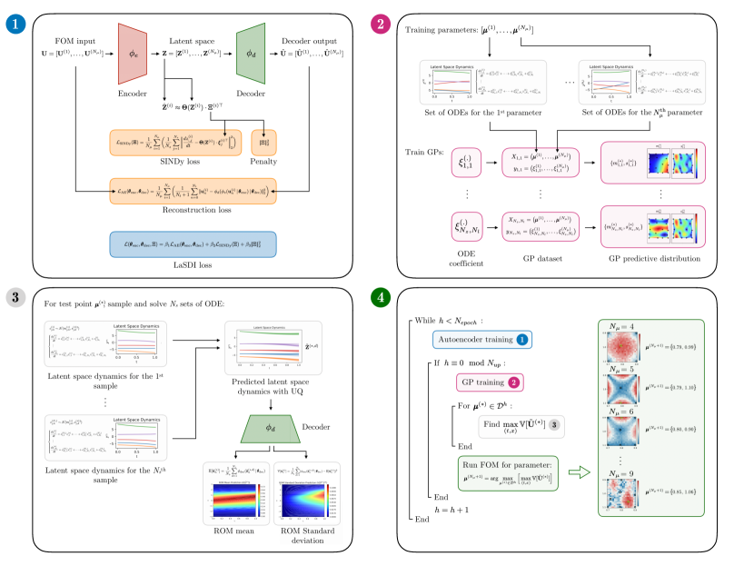
Figure 1: GPLaSDI framework. (1) Autoencoder/SINDy joint-training. (2) GP interpolation. (3) ROM prediction with uncertainty quantification. (4) Active learning strategy.

In order to make ROM predictions for a new test parameter $\boldsymbol{\mu}^{(*)}\in\mathcal{D}$, we need to solve the corresponding set of ODEs, with coefficients $\mathbf{\Xi}^{(*)}$. In LaSDI [11] and gLaSDI [13], $\mathbf{\Xi}^{(*)}$ is estimated through deterministic interpolation of $\mathbf{\Xi}$. In this paper, we propose to use Gaussian Processes (GPs). This has two main advantages: first, GPs are less prone to overfitting, which may provide a more accurate interpolation of the latent space governing dynamics. Second, GPs provide confidence intervals over their predictions. As a result, we can train GPs such that $\mathcal{GP}_{\mathbf{\Xi}}:\boldsymbol{\mu}^{(*)}\mapsto\{m(\mathbf{\Xi}^{(*)}),s(\mathbf{\Xi}^{(*)})\}$, where $m$ and $s$ is the predictive mean and standard deviation of $\mathbf{\Xi}^{(*)}$, respectively. Note that in practice, we train $N_{z}\times N_{l}$ GPs, one for each ODE coefficient. We can than sample sets of ODE coefficients from the predictive Gaussian distribution, $\mathbf{\Xi}^{(*,d)}\sim\mathcal{N}(m(\mathbf{\Xi}^{(*)}),s(\mathbf{\Xi}^{(*)})^{2})$, and integrate each set of ODEs, $\mathbf{\dot{Z}}^{(*,d)}=\mathbf{\Theta}(\mathbf{Z}^{(*,d)})\cdot\mathbf{\Xi}^{(*,d)\top}$, where $d\in[\![1,N_{s}]\!]$ and $N_{s}$ is the number of samples. Each sample set is solved using a numerical integrator (e.g. Forward Euler), and using initial condition $\mathbf{z}_{0}^{(*)}=\phi_{e}(\mathbf{u}_{0}^{(*)}|\mathbf{\theta}_{\text{enc}})$. Finally, we feed each latent space sample dynamics, $\mathbf{\tilde{Z}}^{(*,d)}$ into the decoder to obtain a sample set of ROM predictions. We denote $\mathbb{E}[\mathbf{\tilde{U}}^{(*)}]$ and $\mathbb{V}[\mathbf{\tilde{U}}^{(*)}]$ the ROM mean prediction and variance, respectively.

During the training phase, we adopt a variance-based greedy sampling strategy for active learning. We first train the autoencoder and the SINDy coefficients during $N_{up}$ epochs. Then, GPs are trained over the current set of learned ODE coefficients, $\mathbf{\Xi}$. For a finite number of test point $\boldsymbol{\mu}^{(*)}\in\mathcal{D}^{h}\subset\mathcal{D}$ (where $\mathcal{D}^{h}$ is a discretized subset of the parameter space), we make ROM predictions and perform a new FOM simulation for the test parameter that yielded the highest ROM variance:

$$\boldsymbol{\mu}^{(N_{\mu}+1)}=\arg\max_{\boldsymbol{\mu}^{(*)}\in\mathcal{D}^{h}}\big{[}\max_{(t,x)}\mathbb{V}[\mathbf{\tilde{U}}^{(*)}]\big{]}$$ (4)

The new data point, $\mathbf{U}^{(N_{\mu}+1)}$, is added to the rest of the training set and the training is resumed until the (preset) maximum number of epochs is reached. Figure 1 summarizes the GPLaSDI algorithm.

3 Results and Discussion

We demonstrate the performance of GPLaSDI on a rising bubble problem. A hot fluid bubble is immersed in a colder fluid, causing the bubble to rise-up in a mushroom-like convective pattern. The solved PDE are the coupled compressible unviscid Navier-Stokes, advection-diffusion and energy conservation equations. In this example, implementing the residual would typically be lengthy and cumbersome, showcasing the interest of GPLaSDI.

We consider 2 simulation parameters: the initial bubble temperature, $\theta_{c}$, and its initial radius, $R_{c}$ ($\boldsymbol{\mu}=\{\theta_{c},R_{c}\}$). We employ HyPar [1, 12], a finite-difference PDE solver to perform high fidelity FOM simulations, and the numerical scheme used is described in [15]. We consider a fully connected autoencoder, with softplus activation, a 10100-1000–200–50–20–5 architecture for the encoder, and a symmetric architecture for the decoder ($N_{z}=5$). We use Adam [18], with learning rate $10^{-4}$ over $6.8\cdot 10^{5}$ epochs, and consider a $0.25$ weighing factor for the SINDy loss. We use only linear terms in the SINDy library, and consider $N_{s}=20$ GP samples. We use GPs with RBF kernels, and a greedy sampling rate every $4\cdot 10^{4}$ epochs. For testing purposes, the parameter space is discretized over a $21\times 21$ grid ($\mathcal{D}^{h}$). As for the error metric, we consider the maximum relative error:

$$e(\mathbf{U}^{(*)},\mathbb{E}[\mathbf{\tilde{U}}^{(*)}])=\max(|\!|\mathbb{E}[\mathbf{\tilde{U}}^{(*)}]-\mathbf{U}^{(*)}|\!|_{2}/|\!|\mathbf{U}^{(*)}|\!|_{2})$$ (5)

For baseline comparison, we compare the performance of GPLaSDI with uniform grid sampling. Figure 2.a shows the maximum relative error across the test parameter space $\mathcal{D}^{h}$ with GPLaSDI, and figure 2.b shows the results with uniform grid. With GPLaSDI, the worst maximum relative error is $6.2\%$, and the largest errors occur for parameter values located towards the bottom right corner of the parameter space. GPLaSDI outperforms the baseline, which exhibits higher errors for smaller values of $R_{c}$ ($R_{c}<153$), with the worst maximum relative error reaching $8.3\%$. The model is capable of efficiently sampling data points for which the uncertainty if the highest, and ultimately reduce the prediction error. Figure 2.c shows GPLaSDI maximum predictive standard deviation. It correlates reasonably well with the relative error, confirming that uncertainty-based sampling is effective in reducing model error.

During 20 test runs, the FOM requires an average wall clock run-time of 89.1 seconds when utilizing 16 cores, and 1246.8 seconds when using a single core. On the other hand, the ROM model achieves an average run-time of $1.25\cdot 10^{-2}$ seconds, resulting in an impressive average speed-up of $99,744\times$. Note that this speed up is obtained using only the predictive mean of the GPs for estimating the latent space set of ODEs (i.e. $N_{s}=1$). All the code to reproduce the results in this paper can be found at github.com/LLNL/GPLaSDI.

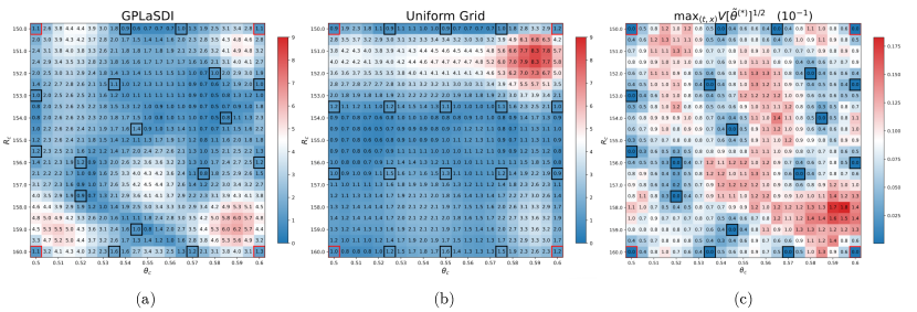
Figure 2: (a) GPLaSDI maximum relative error (in percent). (b) LaSDI with uniform grid sampling maximum relative error. (c) GPLaSDI maximum predictive standard deviation. The 4 corner red boxes represents the parameters used in the initial training dataset. The black boxes represent the parameters sampled during training.

4 Broader Impact

We have introduced GPLaSDI, a fully data-driven non-intrusive ROM algorithm, with an uncertainty-based active learning approach. GPLaSDI is applicable to any type of physics or scientific phenomenon, does not requires direct access of even knowledge of the physical governing equations, and is capable of quantifying its own prediction uncertainty, while achieving remarkable speed-up.

References

- [1] HyPar Repository. https://bitbucket.org/deboghosh/hypar.
- Jou [2020] Review of digital twin about concepts, technologies, and industrial applications. Journal of Manufacturing Systems, 58:346–361, 2020. doi: 10.1016/J.JMSY.2020.06.017.
- BELYTSCHKO [1989] T. BELYTSCHKO. The finite element method: Linear static and dynamic finite element analysis: Thomas j. r. hughes. Computer-Aided Civil and Infrastructure Engineering, 4(3):245–246, 1989. doi: https://doi.org/10.1111/j.1467-8667.1989.tb00025.x. URL https://onlinelibrary.wiley.com/doi/abs/10.1111/j.1467-8667.1989.tb00025.x.
- Berkooz et al. [1993] G. Berkooz, P. Holmes, and J. L. Lumley. The proper orthogonal decomposition in the analysis of turbulent flows. Annual Review of Fluid Mechanics, 25(1):539–575, 1993. doi: 10.1146/annurev.fl.25.010193.002543. URL https://doi.org/10.1146/annurev.fl.25.010193.002543.
- Bonneville and Earls [2022] C. Bonneville and C. Earls. Bayesian deep learning for partial differential equation parameter discovery with sparse and noisy data. Journal of Computational Physics: X, 16:100115, 2022. ISSN 2590-0552. doi: https://doi.org/10.1016/j.jcpx.2022.100115. URL https://www.sciencedirect.com/science/article/pii/S2590055222000117.
- Brunton et al. [2016] S. L. Brunton, J. L. Proctor, and J. N. Kutz. Discovering governing equations from data by sparse identification of nonlinear dynamical systems. Proceedings of the National Academy of Sciences, 113(15):3932–3937, 2016. doi: 10.1073/pnas.1517384113. URL https://www.pnas.org/doi/abs/10.1073/pnas.1517384113.
- Calder et al. [2018] M. Calder, C. Craig, D. Culley, R. Cani, C. Donnelly, R. Douglas, B. Edmonds, J. Gascoigne, N. Gilbert, C. Hargrove, D. Hinds, D. Lane, D. Mitchell, G. Pavey, D. Robertson, B. Rosewell, S. Sherwin, M. Walport, and A. Wilson. Computational modelling for decision-making: Where, why, what, who and how. Royal Society Open Science, 5:172096, 06 2018. doi: 10.1098/rsos.172096.
- Champion et al. [2019] K. Champion, B. Lusch, J. N. Kutz, and S. L. Brunton. Data-driven discovery of coordinates and governing equations. Proceedings of the National Academy of Sciences, 116(45):22445–22451, 2019. doi: 10.1073/pnas.1906995116. URL https://www.pnas.org/doi/abs/10.1073/pnas.1906995116.
- Chen et al. [2021] Z. Chen, Y. Liu, and H. Sun. Physics-informed learning of governing equations from scarce data. Nature Communications, 12(1), oct 2021. doi: 10.1038/s41467-021-26434-1. URL https://doi.org/10.1038%2Fs41467-021-26434-1.
- Diston [2009] D. Diston. Computational Modelling and Simulation of Aircraft and the Environment: Platform Kinematics and Synthetic Environment, volume 1 of Aerospace Series. John Wiley & Sons Ltd, United Kingdom, 1 edition, Apr. 2009. ISBN 9780470018408. doi: 10.1002/9780470744130.
- Fries et al. [2022] W. D. Fries, X. He, and Y. Choi. LaSDI: Parametric latent space dynamics identification. Computer Methods in Applied Mechanics and Engineering, 399:115436, sep 2022. doi: 10.1016/j.cma.2022.115436. URL https://doi.org/10.1016%2Fj.cma.2022.115436.
- Ghosh and Constantinescu [2016] D. Ghosh and E. M. Constantinescu. Well-balanced, conservative finite-difference algorithm for atmospheric flows. AIAA Journal, 54(4):1370–1385, April 2016. doi: 10.2514/1.J054580.
- He et al. [2023] X. He, Y. Choi, W. D. Fries, J. Belof, and J.-S. Chen. gLaSDI: Parametric physics-informed greedy latent space dynamics identification. 489:112267, 2023. doi: 10.1016/j.jcp.2023.112267. URL https://www.sciencedirect.com/science/article/abs/pii/S0021999123003625.
- Hinton and Salakhutdinov [2006] G. E. Hinton and R. R. Salakhutdinov. Reducing the dimensionality of data with neural networks. Science, 313(5786):504–507, 2006. doi: 10.1126/science.1127647. URL https://www.science.org/doi/abs/10.1126/science.1127647.
- Jiang and Shu [1996] G.-S. Jiang and C.-W. Shu. Efficient implementation of weighted ENO schemes. Journal of Computational Physics, 126(1):202–228, 1996. ISSN 0021-9991. doi: 10.1006/jcph.1996.0130.
- Jones et al. [2020] D. Jones, C. Snider, A. Nassehi, J. Yon, and B. Hicks. Characterising the digital twin: A systematic literature review. CIRP Journal of Manufacturing Science and Technology, 29:36–52, 2020. ISSN 1755-5817. doi: https://doi.org/10.1016/j.cirpj.2020.02.002. URL https://www.sciencedirect.com/science/article/pii/S1755581720300110.
- Kim et al. [2020] Y. Kim, Y. Choi, D. Widemann, and T. Zohdi. A fast and accurate physics-informed neural network reduced order model with shallow masked autoencoder, 2020. URL https://arxiv.org/abs/2009.11990.
- Kingma and Ba [2014] D. P. Kingma and J. Ba. Adam: A method for stochastic optimization, 2014. URL https://arxiv.org/abs/1412.6980.
- Kutz [2017] J. N. Kutz. Deep learning in fluid dynamics. Journal of Fluid Mechanics, 814:1–4, 2017. doi: 10.1017/jfm.2016.803.
- Lee and Carlberg [2020] K. Lee and K. T. Carlberg. Model reduction of dynamical systems on nonlinear manifolds using deep convolutional autoencoders. Journal of Computational Physics, 404:108973, 2020. ISSN 0021-9991. doi: https://doi.org/10.1016/j.jcp.2019.108973. URL https://www.sciencedirect.com/science/article/pii/S0021999119306783.
- Raczynski [2006 - 2006] S. Raczynski. Modeling and simulation : the computer science of illusion / Stanislaw Raczynski. RSP Series in Computer Simulation and Modeling. John Wiley & Sons, Ltd, Hertfordshire, England ;, 2006 - 2006. ISBN 0-470-03089-5.
- Rozza et al. [2007] G. Rozza, D. Huynh, and A. Patera. Reduced basis approximation and a posteriori error estimation for affinely parametrized elliptic coercive partial differential equations. Archives of Computational Methods in Engineering, 15:1–47, 09 2007. doi: 10.1007/BF03024948.
- Rudy et al. [2017] S. H. Rudy, S. L. Brunton, J. L. Proctor, and J. N. Kutz. Data-driven discovery of partial differential equations. Science Advances, 3(4):e1602614, 2017. doi: 10.1126/sciadv.1602614. URL https://www.science.org/doi/abs/10.1126/sciadv.1602614.
- Safonov and Chiang [1988] M. G. Safonov and R. Y. Chiang. A schur method for balanced model reduction. 1988 American Control Conference, pages 1036–1040, 1988.
- Stephany and Earls [2022] R. Stephany and C. Earls. Pde-read: Human-readable partial differential equation discovery using deep learning. Neural Networks, 154:360–382, 2022. ISSN 0893-6080. doi: https://doi.org/10.1016/j.neunet.2022.07.008. URL https://www.sciencedirect.com/science/article/pii/S0893608022002660.
- Winsberg [2022] E. Winsberg. Computer Simulations in Science. In E. N. Zalta and U. Nodelman, editors, The Stanford Encyclopedia of Philosophy. Metaphysics Research Lab, Stanford University, Winter 2022 edition, 2022.