Observational Constraints on Extended Starobinsky and Weyl Gravity Model of Inflation

Abstract

We present constraints on the extended Starobinsky and Weyl gravity model of inflation using updated available observational data. The data includes cosmic microwave background (CMB) anisotropy measurements from Planck and BICEP/Keck 2018 (BK18), as well as large-scale structure data encompassing cosmic shear and galaxy autocorrelation and cross-correlation functions measurements from Dark Energy Survey (DES), baryonic acoustic oscillation (BAO) measurements from 6dF, MGS and BOSS, and distance measurements from supernovae type Ia from Pantheon+ samples. By introducing a single additional parameter, each model extends the Starobinsky model to encompass larger region of parameter space while remaining consistent with all observational data. Specifically for higher number of $e$-folding, these models extend viable range of tensor-to-scalar ratio ($r$) to very small value $r<0.001$ in contrast to the original $R^{2}$ Starobinsky model. In addition, our results continue to emphasize the tension in $H_{0}$ and $S_{8}$ between early-time CMB measurements and late-time large-scale structure observations.

1 Introduction

The Starobinsky model is one of the simplest models of inflation that is consistent with observational constraints from Planck Cosmic Microwave Background radiation 2018 (Planck Collaboration et al., 2020a). The model contains one-loop quantum gravity correction which naturally leads to an $R^{2}$ term in the effective gravity action, in addition to the Einstein-Hilbert linear action term (Starobinsky, 1980; Antoniadis & Patil, 2015). The loop contribution is expected to be significant in the very early universe since Planckian physics inevitably introduce higher order terms in the form of $R^{n}$, amongst the other possible Lorentz invariant combinations, into the effective gravity action (see Burgess (2004) for a nice review). These higher order terms should play an important role in very early stage of the universe, potentially causing and governing the inflationary era.

A phenomenological attempt to consider the effects of $R^{3}$ term is proposed in Cheong et al. (2020) where the coefficient of the extra term is taken to be a free small parameter with respect to the $R^{2}$ contribution. In contrast, a conformal Weyl inflation model is proposed in Wang et al. (2023) with different structure of the $R^{2}$ and $R^{3}$ terms. Both models can be set to reduce to conventional Starobinsky model but their extensions to the $R^{3}$ contribution are different and deserve detailed comparison with respect to the updated observational data. In this work, we consider constraints from Planck CMB 2018 (TTTEEE+lowE+lensing), BK18 (Bicep Keck 2018) (Ade et al., 2021), large-scale structure data, i.e., BAO (Baryon Acoustic Oscillation) (Alam et al., 2017), DES (Dark Energy Servey) (Abbott et al., 2018), and low-redshift Pantheon+ supernovae type Ia sample (Scolnic et al., 2022) to the parameter space of Starobinsky, $R^{3}$ extended Starobinsky, and Weyl gravity model of inflation.

This work is organized as follows: In Sec. 2, we provide a review of the basic scalar-tensor gravity theory and extended Starobinsky model. Subsequently, we compute the inflationary model parameters. In Sec. 3, we introduce Weyl gravity model of inflation along with the relevant inflationary parameters. We explain the data analysis and provide a concise overview of the data we employed in Sec. 4. The results are presented in Sec. 5. We discuss our results and provide a conclusing summary in Sec. 6.

2 The scalar-tensor gravity theory and Starobinsky models

We start with an overview of the well-known results in scalar-tensor gravity theory. In the Jordan frame, the action of matter and generic $f(R)$ gravity can be expressed as

$$S = S_{\rm J}+S_{m}(g_{{\rm J}\mu\nu},\Psi_{m}),$$ (1)

$$= \frac{1}{2\kappa^{2}}\int{\,\textrm{d}^{4}x\sqrt{-g_{\rm J}}f(R_{\rm J})}+S_{m}(g_{{\rm J}\mu\nu},\Psi_{m}),$$

where $\kappa^{2}=8\pi G=1$, $S_{m}$ is a matter action with fields $\Psi_{m}$ and $g_{\rm J}$ is the determinant of the space-time metric $g_{\rm J\mu\nu}$. Performing the Legendre transformation to the gravity part of the action gives rise to

$$S_{\rm J}=\frac{1}{2}\int{\,\textrm{d}^{4}x\sqrt{-g_{\rm J}}[F(R_{\rm J})R_{\rm J}-U(R_{\rm J}))]},$$ (2)

where $F(R_{\rm J})\equiv\partial f/\partial R_{\rm J}$ and $U(R_{\rm J})=F(R_{\rm J})R_{\rm J}-f(R_{\rm J})$.

The $f(R)$ gravity is equivalent to the scalar-tensor theory by a conformal transformation

$$g_{\rm E\mu\nu}=\Omega^{2}g_{\rm J\mu\nu}\rightarrow\sqrt{-g_{\rm E}}=\Omega^{4}\sqrt{-g_{\rm J}},$$ (3)

where $\Omega^{2}$ is a conformal factor. Under the transformation, we obtain the transformed Ricci scalar

$$R_{\rm J} = \Omega^{2}R_{\rm E}+6g_{\rm E}^{\mu\nu}\Omega(\partial_{\mu}\partial_{\nu}\Omega)-12g_{\rm E}^{\mu\nu}(\partial_{\mu}\Omega)(\partial_{\nu}\Omega)$$ (4)

$$\equiv \Omega^{2}[R_{\rm E}-g_{\rm E}^{\mu\nu}(\partial_{\mu}s)(\partial_{\nu}s)],$$

where $s$ is a canonical field. The gravity action in the Einstein frame then takes the form

$$S_{\rm E}=\int{\,\textrm{d}^{4}x\sqrt{-g_{\rm E}}\bigg{[}\frac{1}{2}R_{\rm E}-\frac{1}{2}g_{\rm E}^{\mu\nu}\partial_{\mu}s\partial_{\nu}s-V_{\rm E}(s)\bigg{]}}.$$ (5)

where we choose

$$\Omega^{2}(\phi)=F(R_{\rm J})=f^{\prime}(R_{\rm J})=f^{\prime}(\phi),$$ (6)

and a new scalar field $R_{\rm J}\equiv\phi$ is defined. The canonical field $s(\phi)$ can then be expressed as

$$s(\phi)=\sqrt{\frac{3}{2}}\ln{\Omega^{2}(\phi)}=\sqrt{\frac{3}{2}}\ln{[f^{\prime}(\phi)]}.$$ (7)

And the potential in the Einstein frame is

$$V_{\rm E}(s)=\frac{U(R_{\rm J})}{2\Omega^{4}} = \frac{F(R_{\rm J})R_{\rm J}-f(R_{\rm J})}{2\Omega^{4}}$$ (8)

$$= \frac{\phi f^{\prime}(\phi)-f(\phi)}{2f^{\prime}(\phi)^{2}}\Big{|}_{\phi=\phi(s)}.$$

2.1 The extended Starobinsky model

First, we review the extended Starobinsky model studied in Cheong et al. (2020) where a slightly different approximation with respect to the $e$-folding number $N_{\rm e}$ is used in our calculation in Sec. 2.2. Start with

$$f(R)=aR+bR^{2}+cR^{3},$$ (9)

where $a=1$, $b=\displaystyle{\frac{\beta}{2}}$ and $c=\displaystyle{\frac{\gamma}{3}}$. The conformal factor becomes

$$\Omega^{2}(\phi)=f^{\prime}(\phi)=1+\beta\phi^{2}+\gamma\phi^{3}.$$ (10)

Substitute into Eq. (7) to obtain $s(\phi)$

$$s(\phi)=\sqrt{\frac{3}{2}}\ln{[1+\beta\phi+\gamma\phi^{2}]},$$

and define the quadratic field of scalar

$$\sigma(s)\equiv\exp\left(\sqrt{\frac{2}{3}}s\right)=1+\beta\phi+\gamma\phi^{2}.$$ (11)

The $\phi(s)$ can be solved as a solution of the quadratic equation

$$\phi(s)=\frac{\beta}{2\gamma}\left(\sqrt{1+4\frac{\gamma}{\beta^{2}}(\sigma(s)-1)}-1\right).$$ (12)

Consider if $\gamma\ll\beta$ and $\phi\approx 1$, we impose $\gamma$ as a small perturbation in $\sigma(s)$, so that

$$\beta\phi(s)+1=\sigma(s)-\frac{\gamma}{\beta^{2}}(\sigma(s)-1)^{2}+\cdots.$$

Solve the equation above to obtain $\phi(s)$

$$\phi(s)=\frac{\sigma(s)-1}{\beta}\left[1-\frac{\gamma}{\beta}\left(\frac{\sigma(s)-1}{\beta}\right)+\mathcal{O}\left(\frac{\gamma}{\beta}\right)^{2}\right].$$ (13)

The potential in Einstein frame Eq. (8) then becomes

$$V_{\rm E}(s) =\frac{\beta\phi(s)^{2}(1+\frac{4\gamma}{3\beta})}{4(1+\beta\phi(s)(1+\frac{\gamma}{\beta}\phi(s)))^{2}}$$ (15)

$$\approx V_{0}(s)\left[1-\frac{2\gamma}{3\beta}\left(\frac{\sigma(s)-1}{\beta}\right)+\cdots\right],$$

where $V_{0}(s)=\displaystyle{\frac{1}{4\beta}\left(1-\frac{1}{\sigma}\right)^{2}=\frac{1}{4\beta}\left(1-e^{-\sqrt{\frac{2}{3}}s}\right)^{2}}$ for $\gamma=0$ .

2.2 The slow-roll inflation

The slow-roll parameters can be approximate to the leading order of $\mathcal{O}(\gamma/\beta)$ as

$$\epsilon = \frac{1}{2}\left(\frac{V^{\prime}_{\rm E}}{V_{\rm E}}\right)^{2}=\epsilon_{0}+\frac{\gamma}{\beta}\Delta\epsilon$$ (16)

$$\eta = \frac{V^{\prime\prime}_{\rm E}}{V_{\rm E}}=\eta_{0}+\frac{\gamma}{\beta}\Delta\eta,$$ (17)

where $\epsilon_{0}$ and $\eta_{0}$ are the slow-roll parameters for $\gamma=0$ and we calculate them in terms of perturbation

$$\epsilon_{0} = \frac{4}{3(\sigma(s)-1)^{2}}$$ (18)

$$\eta_{0} = -\frac{4(\sigma(s)-2)}{3(\sigma(s)-1)^{2}}$$ (19)

$$\Delta\epsilon = -\frac{8\sigma(s)}{9\beta(\sigma(s)-1)}+\mathcal{O}\left(\frac{\gamma}{\beta}\right)$$ (20)

$$\Delta\eta = -\frac{4\sigma(s)(\sigma(s)+3)}{9\beta(\sigma(s)-1)}+\mathcal{O}\left(\frac{\gamma}{\beta}\right).$$ (21)

The number of $e$-foldings from the start to the end of inflation $(s_{\rm e}<s)$ can then be determined

$$N_{\rm e}(s) = \int^{s}_{s_{e}}\frac{\,\textrm{d}s}{\sqrt{2\epsilon}}=N_{\rm e,0}+\Delta N_{\rm e},$$ (22)

$$\approx \frac{3}{4}\sigma(s)+\left(\frac{\gamma}{\beta}\right)\frac{\sigma(s)^{3}}{12\beta}$$

where $N_{\rm e,0}$ is $e$-folding number for $\gamma=0$ and $\Delta N_{\rm e}$ is correction at the leading order $\gamma/\beta$ and assuming $s\gg s_{e}\sim 1$.

For $N_{e}$ $e$-foldings at $s_{*}$,

$$N_{\rm e}(s_{*})=\frac{3}{4}\sigma(s_{*})+\left(\frac{\gamma}{\beta}\right)\frac{\sigma(s_{*})^{3}}{12\beta}.$$ (23)

The asymptotic solution of $\sigma(s_{*})$ for generic $N_{e}$ is thus

$$\sigma(s_{*})\approx\frac{4}{3}N_{\rm e}-\delta\frac{64}{243}N_{\rm e}^{3},$$ (24)

where $\delta\equiv\gamma/\beta^{2}\ll 1$.

The primordial power spectra (scalar and tensor mode) are parameterized in power-law forms as follows:

$$\ln\mathcal{P}_{\rm s}(k)=\ln A_{\rm s}+(n_{\rm s}-1)\ln\left(\frac{k}{k_{*}}\right)+\frac{1}{2}\frac{{\rm d}\ln n_{\rm s}}{{\rm d}\ln k}\ln\left(\frac{k}{k_{*}}\right)^{2}+\frac{1}{6}\frac{{\rm d}^{2}\ln n_{\rm s}}{{\rm d}\ln k^{2}}\ln\left(\frac{k}{k_{*}}\right)^{3}+\ldots$$ (25)

and

$$\ln\mathcal{P}_{\rm t}(k)=\ln(rA_{\rm s})+n_{\rm t}\ln\left(\frac{k}{k_{*}}\right)++\frac{1}{2}\frac{{\rm d}\ln n_{\rm t}}{{\rm d}\ln k}\ln\left(\frac{k}{k_{*}}\right)^{2}+\ldots,$$ (26)

where $\mathcal{P}_{\rm s}$ and $\mathcal{P}_{\rm t}$ are the scalar and tensor power spectrum respectively. $n_{\rm s}$ and $n_{\rm t}$ are the scalar and tensor spectral index. $r$ is the tensor-to-scalar ratio and $A_{\rm s}$ is the primordial scalar power spectrum amplitude. We define the running and running of running of the corresponding parameters as $\displaystyle n_{\rm run}\equiv{\rm d}\ln n_{\rm s}/{\rm d}\ln k$, $\displaystyle n_{\rm run,run}\equiv{\rm d}^{2}\ln n_{\rm s}/{\rm d}\ln k^{2}$ and $n_{\rm t,run}\equiv{\rm d}\ln n_{\rm t}/{\rm d}\ln k$.

The observable cosmological parameters are obtained in terms of two free parameters $N_{\rm e}$ and $\delta$. The scalar spectral index is given explicitly by

$$n_{\rm s} =1-6\epsilon(s_{*})+2\eta(s_{*})$$ (27)

$$=\frac{16N_{\rm e}^{2}-56N_{\rm e}-15}{(4N_{\rm e}-3)^{2}}$$

$$-\delta\frac{32(256N_{\rm e}^{4}-576N_{\rm e}^{3}+756N_{\rm e}^{2}-243N_{\rm e})}{81(4N_{\rm e}-3)^{3}}.$$

Note that we keep the full dependence on $N_{\rm e}$. The tensor to scalar ratio is thus

$$r =16\epsilon(s_{*})$$

$$=\frac{192}{(4N_{\rm e}-3)^{2}}-\delta\frac{512(32N_{\rm e}^{3}-72N_{\rm e}^{2}+27N_{\rm e})}{27(4N_{\rm e}-3)^{3}}.$$

Moreover the running of scalar spectral index is

$$n_{\rm run} =\alpha_{s}=\frac{\,\textrm{d}n_{\rm s}}{\,\textrm{d}\log k}=-2\xi+16\epsilon\eta-24\epsilon^{2}$$

$$=-\frac{128(4N_{\rm e}^{2}+9N_{\rm e})}{(4N_{\rm e}-3)^{4}}$$

$$+\delta\frac{128(1024N_{\rm e}^{5}-3840N_{\rm e}^{4}+864N_{\rm e}^{3}-1620N_{\rm e}^{2}+729N_{\rm e})}{81(4N_{\rm e}-3)^{5}},$$

and the running of running of scalar spectral index is given by

$$n_{\rm run,run}=\beta_{s} =\frac{d\alpha_{s}}{d\log k}=-2\omega-2\eta\xi+24\epsilon\xi+32\epsilon\eta^{2}-192\epsilon^{2}\eta+192\epsilon^{3}$$ (30)

$$=\frac{512(32N_{\rm e}^{3}+132N_{\rm e}^{2}+27N_{\rm e})}{(4N_{\rm e}-3)^{6}}$$

$$+\delta\frac{512(2048N_{\rm e}^{5}+20352N_{\rm e}^{4}+864N_{\rm e}^{3}-1620N_{\rm e}^{2}-729N_{\rm e})}{27(4N_{\rm e}-3)^{7}},$$

where Liddle & Lyth (2000)

$$\xi \equiv \displaystyle{\frac{V^{\prime}_{\rm E}V^{\prime\prime\prime}_{\rm E}}{V_{\rm E}^{2}}}=\frac{16(\sigma-4)}{9(\sigma-1)^{3}}-\delta\frac{16\sigma\left(2\sigma^{2}-7\sigma+11\right)}{27(\sigma-1)^{3}},$$

$$\omega \equiv \displaystyle{\frac{V^{\prime}_{\rm E}{}^{2}V^{\prime\prime\prime\prime}_{\rm E}}{V_{\rm E}^{3}}}=-\frac{64(\sigma-8)}{27(\sigma-1)^{4}}+\delta\frac{64\sigma\left(\sigma^{2}-20\sigma+31\right)}{81(\sigma-1)^{4}}.$$

The tensor spectral index can also be computed,

$$n_{\rm t} =-2\epsilon$$

$$=-\frac{24}{(4N_{\rm e}-3)^{2}}+\delta\frac{64(32N_{\rm e}^{3}-72N_{\rm e}^{2}+27N_{\rm e})}{27(4N_{\rm e}-3)^{3}}.$$

And the running of tensor spectral index takes the form,

$$n_{\rm t,run} =4\epsilon\eta-8\epsilon^{2}$$ (32)

$$=-\frac{768N_{\rm e}}{\left(4N_{\rm e}-3\right)^{4}}$$

$$-\delta\frac{256\left(64N_{\rm e}^{3}+36N_{\rm e}^{2}-27N_{\rm e}\right)}{9\left(4N_{\rm e}-3\right){}^{5}}.$$

For $\delta=0$, the Starobinsky model $aR+bR^{2}$ is recovered,

$$n_{\rm s} =\frac{16N_{\rm e}^{2}-56N_{\rm e}-15}{(4N_{\rm e}-3)^{2}}\simeq 1-\frac{2}{N_{\rm e}}-\frac{9}{2N_{\rm e}^{2}},$$ (33)

$$r =\frac{192}{(4N_{\rm e}-3)^{2}}\simeq\frac{12}{N_{\rm e}^{2}}.$$ (34)

3 Weyl Gravity Model

In comparison to the extended Starobinsky model discussed above, there is another type of extension which contains $R^{2}$ and $R^{3}$ terms, the Weyl gravity (WG) model. WG model contains additional Weyl scalar and vector fields whence transition to Einstein gravity is achieved after conformal symmetry breaking. On the galactic scale, Weyl (geometric) gravity models (Ghilencea, 2019a; Ghilencea & Lee, 2019; Ghilencea, 2019b, 2020a, 2020b, 2021; Ghilencea & Harko, 2021; Ghilencea, 2022, 2023; Weißwange et al., 2023) provides alternative possibility of/to dark matter as a successful quantitative description of the galaxy rotation curves (Burikham et al., 2023).

Details of the inflationary scenario of a class of WG model are explored in Wang et al. (2023) where two inflation scenarios are considered, inflation to the side and inflation to the center. Here we consider only the inflation to the side scenario with $\zeta\to\infty$.

For Weyl gravity action, the transformation to Einstein frame of the $f(R)$ gravity in Sect. 2 can be generically performed with replacement

$$\frac{f(R_{\rm J})}{\kappa^{2}}\to F(R_{\rm J},\varphi)-\zeta D^{\mu}\varphi D_{\mu}\varphi-\frac{1}{2g_{\rm W}^{2}}F_{\mu\nu}F^{\mu\nu},$$ (35)

where $F_{\mu\nu}=\partial_{\mu}W_{\nu}-\partial_{\nu}W_{\mu}$ for

$$F(R_{\rm J},\varphi) = \varphi^{2}R_{\rm J}+\alpha R_{\rm J}^{2}+\frac{\beta}{\varphi^{2}}R_{\rm J}^{3}.$$ (36)

This leads to Tang & Wu (2020); Wang et al. (2023)

$$\frac{\mathcal{L}}{\sqrt{-g_{\rm E}}} = \frac{R}{2}-V_{\rm E}(\varphi)-\frac{\partial_{\mu}\varphi\partial^{\mu}\varphi}{2/\zeta+\varphi^{2}/3}-\frac{1}{4g_{\rm W}^{2}}F_{\mu\nu}F^{\mu\nu}$$ (37)

$$+h(\varphi,\zeta,W_{\mu}),$$

where $h(\varphi,\zeta,W_{\mu})$ and $V_{\rm E}(\varphi)$ are given in Eqn. (8) and (9) of Wang et al. (2023) respectively.

The potential in the Einstein frame in $\zeta\to\infty$ limit is then given by

$$V_{\rm E}(\Phi) = \frac{1}{8\alpha}\left(1-e^{\sqrt{\frac{2}{3}}\left(\Phi-\Phi_{0}\right)}\right)^{2}$$

$$\times\left(1+\frac{1}{6}\left(1-e^{-\sqrt{\frac{2}{3}}\left(\Phi-\Phi_{0}\right)}\right)\gamma_{\rm W}\right)+\mathcal{O}(\gamma_{\rm W}^{2}),$$

where $\gamma_{\rm W}\equiv\displaystyle{\frac{3\beta}{\alpha^{2}}}$ and the scalar field is redefined by

$$\varphi^{2}\equiv\frac{6}{|\zeta|}\sinh^{2}\left(\frac{\pm\Phi}{\sqrt{6}}\right).$$ (39)

We can approximate

$$\Phi-\Phi_{0}\approx-\sqrt{\frac{3}{2}}\ln\Bigg{|}\sqrt{\frac{12}{\gamma_{\rm W}}\tanh\Big{(}\tanh^{-1}(0.622\gamma_{\rm W})+\sqrt{\frac{4\gamma_{\rm W}}{27}}(N_{\rm e}+2.7})\Big{)}\Bigg{|}\equiv\sqrt{\frac{3}{2}}\ln\Theta(\gamma_{\rm W},N_{\rm e})$$ (40)

for $N_{\rm e}=50-80$ with a slight change of the constant $2.7$ which do not affect the approximation significantly. The cosmological parameters in this model can be straightforwardly computed,

$$n_{\rm s} = \frac{36(\Theta-5)(3\Theta+1)+(\Theta-1)^{2}((\Theta-26)\Theta-5)\gamma_{\rm W}^{2}-60[\Theta((\Theta-5)\Theta+3)+1]\gamma_{\rm W}}{3(\Theta-1)^{2}\left[(\Theta-1)\gamma_{\rm W}-6\right]^{2}},$$ (41)

$$r = \frac{16\left[\left(\Theta^{2}+\Theta-2\right)\gamma_{\rm W}-12\right]^{2}}{3(\Theta-1)^{2}\left[(\Theta-1)\gamma_{\rm W}-6\right)]^{2}},$$ (42)

$$n_{\rm run} = -\frac{8\Theta\left(\left(\Theta^{2}+\Theta-2\right)\gamma_{\rm W}-12\right)}{3(\Theta-1)^{4}\left[(\Theta-1)\gamma_{\rm W}-6\right]^{4}}$$

$$\times\Big{[}(\Theta-1)\gamma_{\rm W}\left(12(\Theta(\Theta+4)+21)+(\Theta-1)\gamma_{\rm W}\left(4(\Theta-6)(\Theta+2)+\left(2\Theta^{2}+\Theta-3\right)\gamma_{\rm W}\right)\right)-144(\Theta+3)\Big{]},$$

$$n_{\rm run,run} = \frac{32\Theta\left(\left(\Theta^{2}+\Theta-2\right)\gamma_{\rm W}-12\right)}{9(\Theta-1)^{6}\left[(\Theta-1)\gamma_{\rm W}-6\right]^{6}}$$ (44)

$$\times\Bigg{[}\left(-10368\Theta^{2}-57024\Theta-15552\right)+\left(11664\Theta^{3}+39312\Theta^{2}-36720\Theta-14256\right)\gamma_{\rm W}$$

$$+\left(72\Theta^{6}-792\Theta^{5}-2520\Theta^{4}-12312\Theta^{3}+29808\Theta^{2}-9072\Theta-5184\right)\gamma_{\rm W}^{2}$$

$$+\left(48\Theta^{7}-180\Theta^{6}+1128\Theta^{5}+1080\Theta^{4}-7992\Theta^{3}+7908\Theta^{2}-1056\Theta-936\right)\gamma_{\rm W}^{3}$$

$$+\left(2\Theta^{8}+10\Theta^{7}-204\Theta^{6}+284\Theta^{5}+550\Theta^{4}-1422\Theta^{3}+920\Theta^{2}-56\Theta-84\right)\gamma_{\rm W}^{4}$$

$$+\left(\Theta^{8}+5\Theta^{7}-24\Theta^{6}+13\Theta^{5}+50\Theta^{4}-81\Theta^{3}+40\Theta^{2}-\Theta-3\right)\gamma_{\rm W}^{5}\Bigg{]},$$

$$n_{\rm t} = -\frac{2\left[\left(\Theta^{2}+\Theta-2\right)\gamma_{\rm W}-12\right]^{2}}{3(\Theta-1)^{2}\left[(\Theta-1)\gamma_{\rm W}-6\right]^{2}},$$ (45)

$$n_{\rm t,run} = -\frac{8\Theta\left(\left(\Theta^{2}+\Theta-2\right)\gamma_{\rm W}-12\right){}^{2}\left[2\left(\Theta^{2}-6\Theta+5\right)\gamma_{\rm W}+(\Theta-1)^{2}\gamma_{\rm W}^{2}+24\right]}{3(\Theta-1)^{4}\left[(\Theta-1)\gamma_{\rm W}-6\right]^{4}}.$$ (46)

The cosmological parameters given in Sec. 2 and Sec. 3 are then subject to observational constraints as discussed in Sec. 5.

Table 1: The datasets employed in our work.

Datasets	References
Planck TTTEEE+lowE+lensing	(Planck Collaboration et al., 2020b)
BICEP/Keck 2018 (BK18)	(Ade et al., 2021)
Baryonic Acoustic Oscillations (BAO)	(Beutler et al., 2011; Ross et al., 2015; Alam et al., 2017)
Dark Energy Survey (DES)	(Abbott et al., 2018)
Pantheon+	(Scolnic et al., 2022)

Table 2: The datasets combination used in our work.

Datasets
Planck
Planck + BK18
Planck + BAO
Planck + DES
Planck + Pantheon+
Planck + BAO + BK18
Planck + BAO + DES

4 Data Analysis

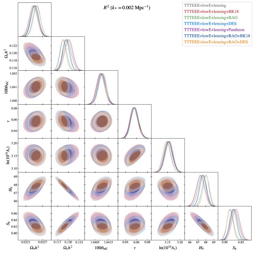
Figure 3: Marginalized 68% and 95% contour plots for the main cosmological parameters for $R^{2}$ Starobinsky model for each dataset in Table 2 for $k_{*}=0.002\ {\rm Mpc}^{-1}$.

We conduct a constraint analysis on the models with a variety of observational data utilizing the Markov Chain Monte Carlo (MCMC) technique (for a recent review see Speagle (2019)) using CosmoMC tool (Lewis & Bridle, 2002). CosmoMC is an MCMC program for exploring cosmological parameter space usually work in conjunction with CAMB, which calculates the CMB power spectra based on input cosmological parameters. We analyse the Markov chains using GetDist tool (Lewis, 2019) which gives the marginalized joint probability constraints on parameters of our interest. The CosmoMC and CAMB codes are modified to incorporate the models by adding the model parameters. For the extended Starobinsky $R^{3}$ model, we add $N_{\rm e}$ and $\delta$ as the model input parameters ($\delta=0$ for the Starobinsky $R^{2}$ model). We apply a uniform prior on $N_{\rm e}\in[50.,80.]$ and $\delta\in[-0.0004,0.0004]$ for the extended Starobinsky $R^{3}$ model. For the Weyl model, we incorporate $N_{\rm e}$ and $\gamma_{\rm W}$ as additional parameters. Similarly, we apply a uniform prior on $N_{\rm e}\in[50.,80.]$ and $\gamma_{\rm W}\in[-1.5\times 10^{-3},1.5\times 10^{3}]$ for Weyl model. The range of our priors are sufficient to encompass the posteriors, as illustrated in Fig. 1 and Fig. 3 - 11.

The power spectrum parameters $n_{\rm s}$, $r$, $n_{\rm run}$, $n_{\rm run,run}$, $n_{\rm t}$ and $n_{\rm t,run}$ are derived from Eqs. (27)–(32) for the extended Starobinsky model. Similar to the extended Starobinsky model, the power spectrum parameters are now derived from Eqs. (41)–(46) for the Weyl model. For each model (Starobinsky and Weyl), we run an analysis with $k_{*}=0.002\ {\rm Mpc}^{-1}$ and $k_{*}=0.05\ {\rm Mpc}^{-1}$ (See equation Eq. (25) and Eq. (26)) respectively. We also give comments on the choice of $k_{*}$ in Sec. 6.5.

We shall provide a concise overview of the data employed in our analysis. The summary of the datasets and dataset combinations used in our work are displayed in Table 1 and Table 2.

4.1 Planck TTTEEE+lowE+lensing

Planck 2018 data release (Planck Collaboration et al., 2020b) comprises a combination of CMB temperature, polarization and lensing anisotropies. The data has been compressed using 2-point statistics, especially the angular correlation function, expressed in terms of the multipole moments $C_{\ell}$ as the final output. There are three types of multipole moments in Planck data: $C_{\ell}^{\rm TT}$, $C_{\ell}^{\rm TE}$ and $C_{\ell}^{\rm EE}$. TT, TE and EE denote temperature auto-correlation, temperature-E-mode polarization cross-correlation and E-mode polarization auto-correlation respectively. In addition, the data also provides an estimate of the power spectrum of the lensing potential and extracted from the data using quadratic estimator (Okamoto & Hu, 2003). The likelihood for temperature and polarization anisotropies measurements use different statistical analysis for large-scale data low-multipole (low-$\ell$ for $2<\ell<30$) and small-scale data high-multipole (high-$\ell$ for $\ell\geq 30$). For low-$\ell$ values, the statistical analysis for the temperature anisotropies is based on the Commander likelihood code. The analysis of low-$\ell$ E-mode polarization likelihood is conducted using the SimAll EE likelihood code and is labelled as lowE. For high values of multipoles moments, the labels TT,TE,EE represent the likelihood analysis for $\ell\geq 30$. For the lensing likelihood analsis the SMICA likelihood is used and is labelled as lensing in Planck data. We adhere to the labelling convention from Planck Collaboration et al. (2020b) for likelihoods, where TTTEEE+lowE+lensing refers to combination of temperature and polarization likelihoods at both high-$\ell$ and low-$\ell$, including the lensing likelihood. In our work, we exclusively utilize the TTTEEE+lowE+lensing Planck data; therefore, when we mention Planck data, we are specifically referring to TTTEEE+lowE+lensing.

4.2 Bicep/Keck 2018 (BK18)

The Bicep/Keck program involves the BICEP (Background Imaging of Cosmic Extragalactic Polarization) instruments working on Keck Array telescopes. Its objective is to detect the B-mode polarization of the CMB. The sources of B-mode polarization mainly come from the primordial gravitational waves and astrophysical foreground, in particular from our own galaxy (Ade et al., 2021). However, both sources emit different B-mode polarization spectra and could be distinguished by multi-frequency measurements. The primordial gravitational wave is generated from the tensor-mode perturbation during the inflation. The BICEP/Keck data complements the Planck dataset and the combined BICEP/Keck and Planck dataset improves the constraint on the tensor-to-scalar ratio $r$. In this work, we employ BICEP/Keck 2018 dataset denoted by BK18.

4.3 Baryonic Acoustic Oscillations (BAO)

The Baryonic Acoustic Oscillations (BAOs) is an imprint of the acoustic waves mediated by baryon-photon plasma during the time of recombination. It has an oscillatory feature in the matter power spectrum that defines characteristic length scale or a standard ruler. The ratio between the tranverse distance to the radial distance also gives a characteristic angular scales at each redshifts. We employ the compilation BAO dataset provided by the CosmoMC package which comprises of the 6dF survey (Beutler et al., 2011) at effective redshift $z_{\rm eff}=0.106$, the SDSS Main Galaxy Sample (Ross et al., 2015) at $z_{\rm eff}=0.15$ and the SDSS III DR12 data (Alam et al., 2017) at $z_{\rm eff}=0.38,0.51,0.61$. The BAO datasets are complimentary to Planck data in terms of temporal coverage.

4.4 Dark Energy Survey (DES)

The primary goal of the Dark Energy Survey (DES) is to investigate the properties of dark energy through a comprehensive approach that includes the analysis of both galaxy clustering and weak gravitational lensing, utilizing correlation functions. This extensive study involves the mapping of more than 300 million galaxies and over ten thousand galaxy clusters, covering an area of over 5,000 square degrees (Abbott et al., 2018). The dataset includes the correlation function of cosmic shear, the angular autocorrelation of luminous red galaxies, and the cross-correlation between the shear of source galaxies and the luminous red galaxy. We employ the DES dataset provided by the CosmoMC package.

4.5 Pantheon+

Pantheon+ is a compilation program of all distance measurements of spectroscopically confirmed Type Ia supernovae (SNIa) to date. The data comprises of 1701 light curves and distance modulus of SNIa (Scolnic et al., 2022). The main goal of the project is to achieve high precision measurements of $H_{0}$ by calibrating with the low-redshift Cepheid variables data from SH0ES program (Supernovae and H0 for the Equation of State of dark energy) (Riess et al., 2022). In our work, we modified CosmoMC and CAMB by employing the distance modulus along with the covariance matrix from Pantheon+ for the likelihood analysis.

5 Results

In this section, we provide constraints on our models described in Sec. 2 and Sec. 3. For each model, an MCMC analysis described in Sec. 4 is performed with the data combination in Table 2. The standard $\Lambda$CDM model with the same setting is also included for comparison. We divide our results into the main parameters which include $\Omega_{\rm b}h^{2}$, $\Omega_{\rm c}h^{2}$, $100\theta_{\rm MC}$, $\tau$, $\ln(10^{10}A_{\rm s})$, $S_{8}$ and $H_{0}$. The power spectrum parameters include $n_{\rm s}$, $r$, $n_{\rm run}$, $n_{\rm run,run}$, $n_{t}$ and $n_{\rm t,run}$. The results for the main parameters are summarized in Table 4 - 7 for $k_{*}=0.002,0.05\ {\rm Mpc}^{-1}$ in Sec. A.1, the results for the power spectrum parameters are summarized in Table 8 - 11 for $k_{*}=0.002,0.05\ {\rm Mpc}^{-1}$.

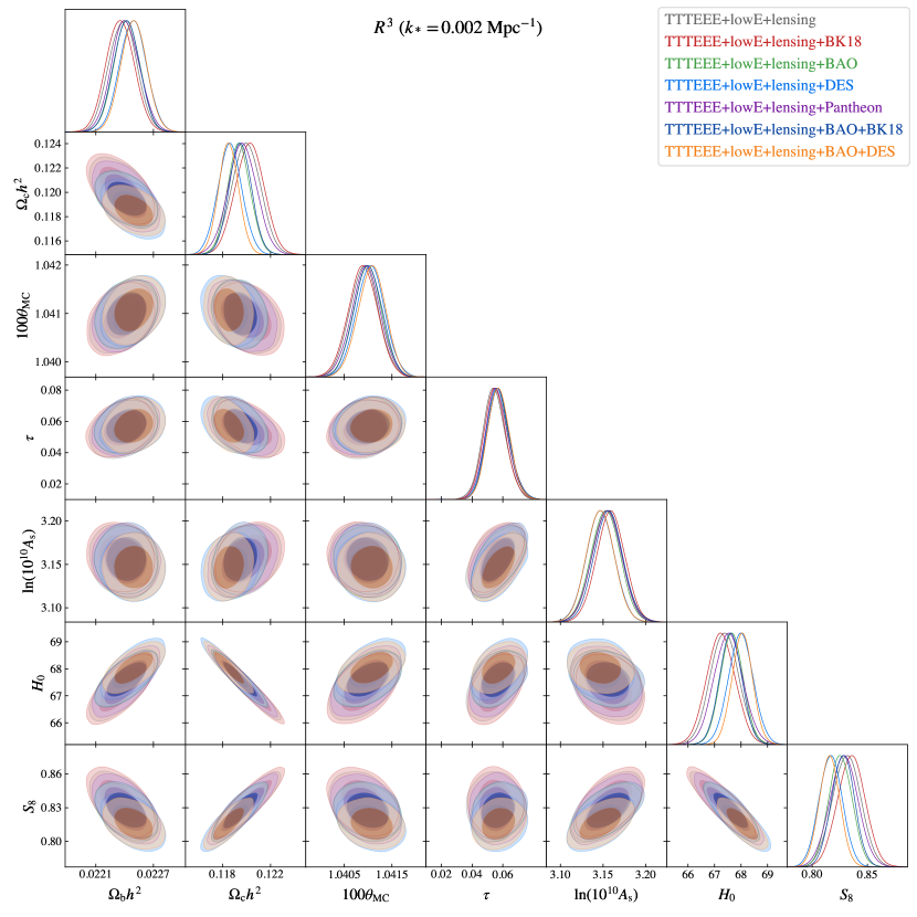
Figure 4: Same as Fig. 3 but for $R^{3}$ Starobinsky model.

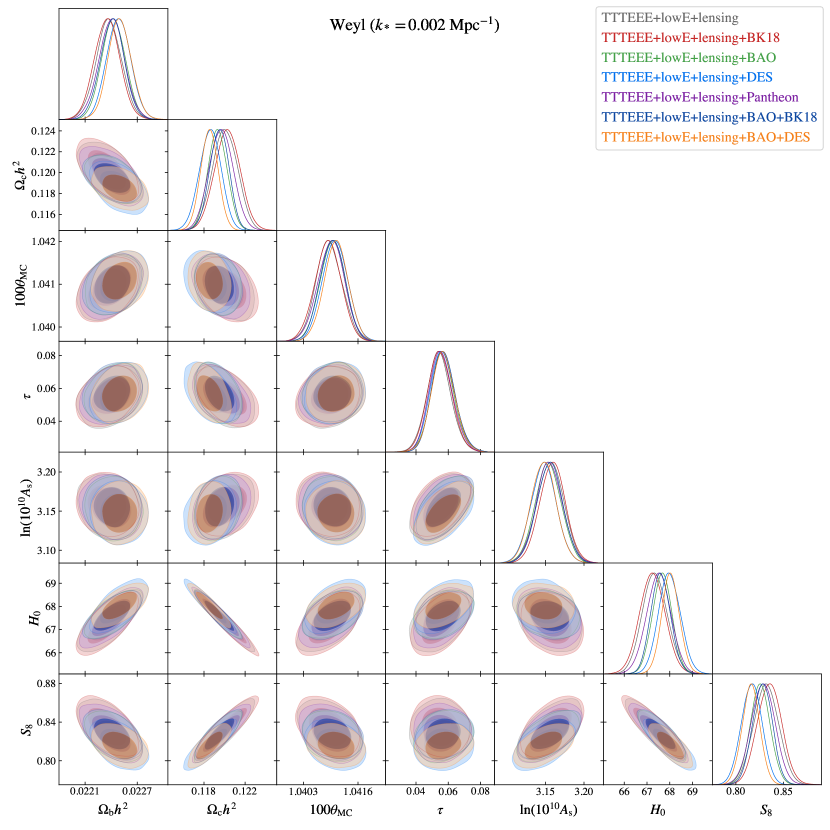
Figure 5: Same as Fig. 3 but for Weyl model.

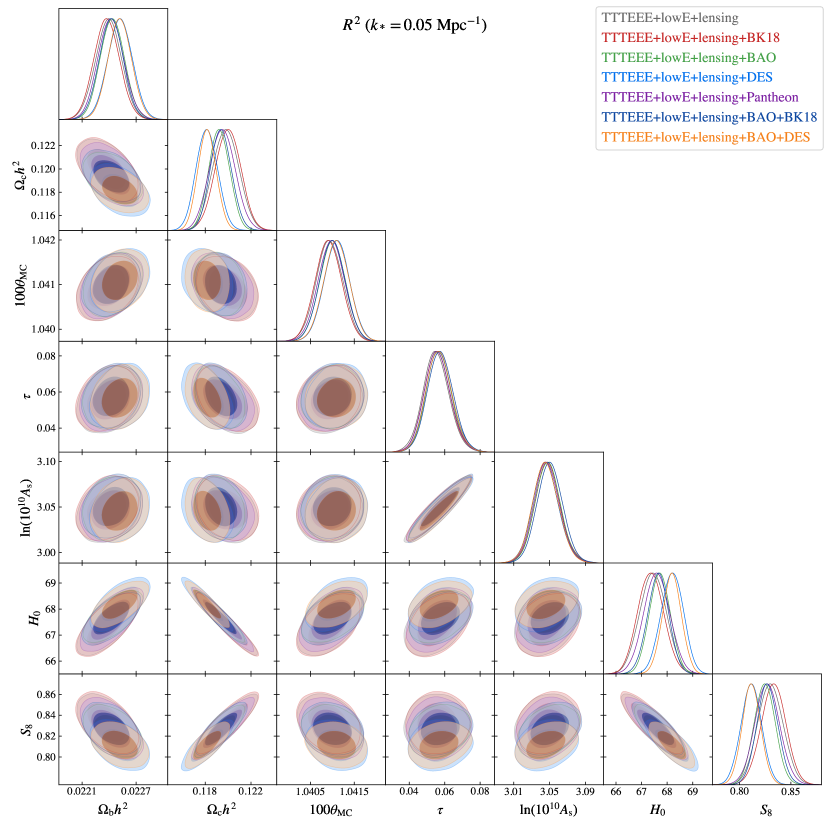
Figure 6: Marginalized 68% and 95% contour plots for the main cosmological parameters for $R^{2}$ Starobinsky model for each dataset in Table 2 for $k_{*}=0.05\ {\rm Mpc}^{-1}$.

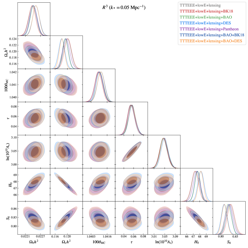
Figure 7: Same as Fig. 6 but for $R^{3}$ Starobinsky model.

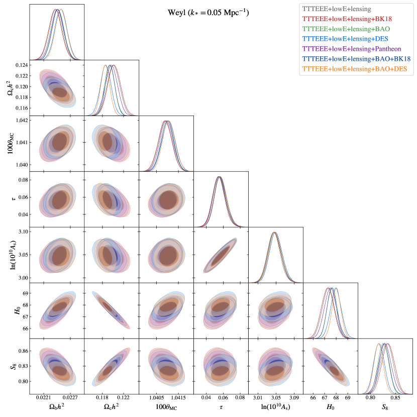
Figure 8: Same as Fig. 6 but for Weyl model.

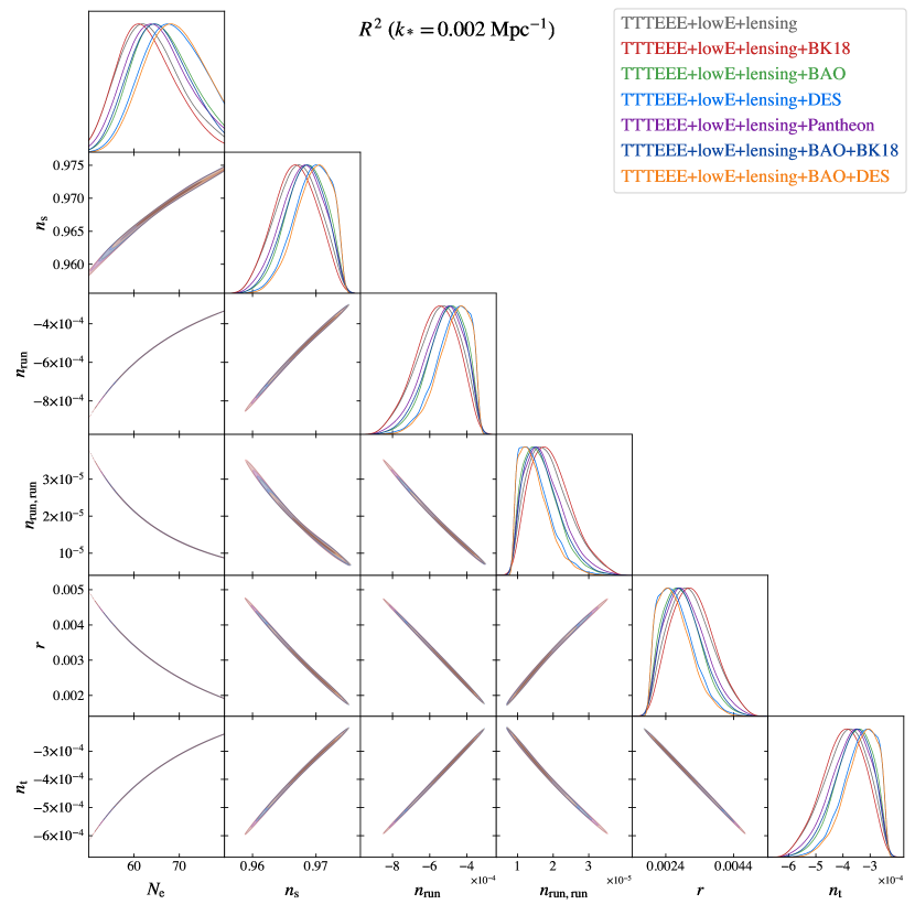
Figure 9: Marginalized 68% and 95% contour plots for the power spectrum parameters for $R^{2}$ Starobinsky model for each dataset in Table 2 for $k_{*}=0.002\ {\rm Mpc}^{-1}$.

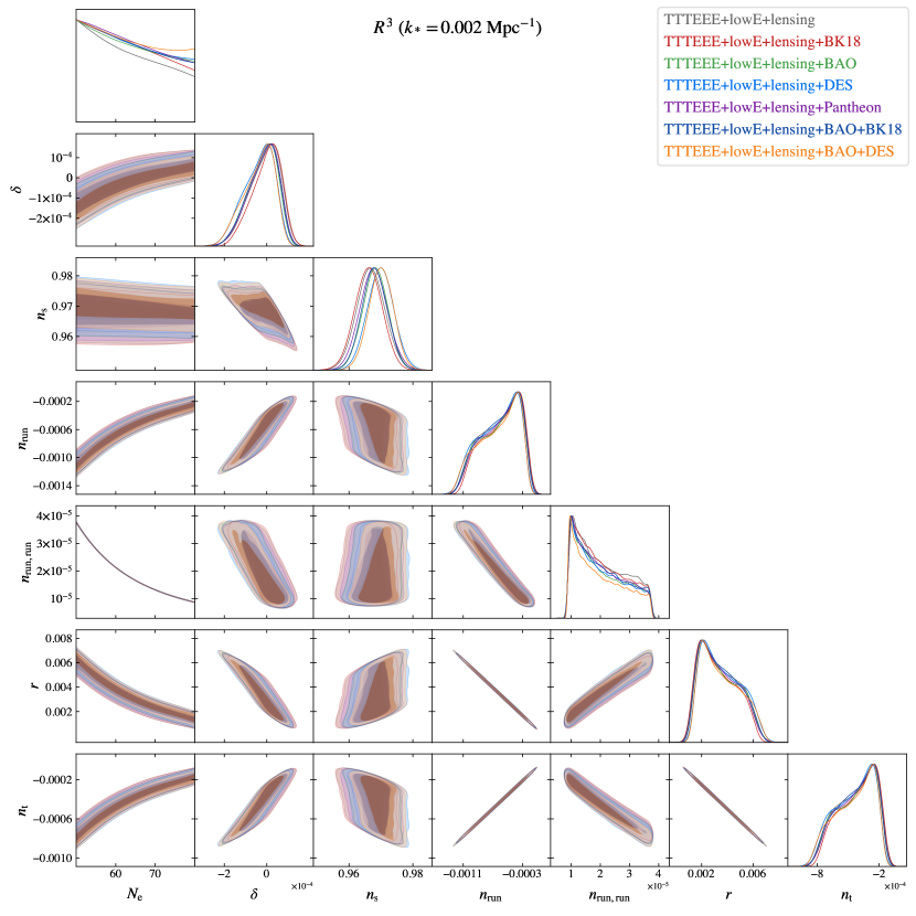
Figure 10: Same as Fig. 9 but for $R^{3}$ Starobinsky model.

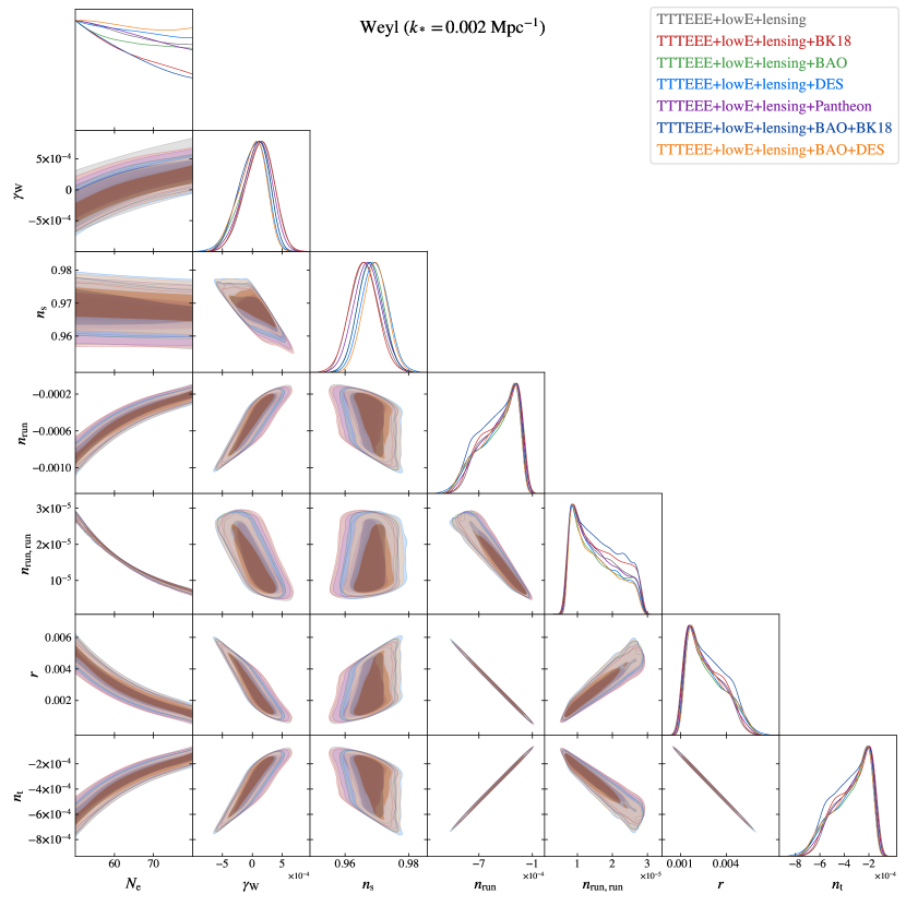
Figure 11: Same as Fig. 9 but for Weyl model.

The marginalized joint 68% and 95% probability regions for the main parameters, $k_{*}=0.002\ {\rm Mpc}^{-1}$, are shown in Fig. 3, Fig. 4 and Fig. 5 in Sec. A.1 for the Starobinsky $R^{2}$, $R^{3}$ and Weyl model respectively. Similarly, the marginalized joint 68% and 95% probability regions for the main parameters, $k_{*}=0.05\ {\rm Mpc}^{-1}$, are shown in Fig. 6, Fig. 7 and Fig. 8 in Sec. A.1. The marginalized joint 68% and 95% probability regions for the power spectrum parameters are also shown in Fig. 9, Fig. 10 and Fig. 11 for $k_{*}=0.002\ {\rm Mpc}^{-1}$ in Sec. A.2.

We also display the constraints on the parameter that are specific to each model ($N_{\rm e}$, $\delta$ or $\gamma_{\rm W}$) in Table 3 for $k_{*}=0.002\ {\rm Mpc}^{-1}$ and $k_{*}=0.05\ {\rm Mpc}^{-1}$ respectively. In additional, we plot the marginalized 68% and 95% constraint on $n_{\rm s}$ and $r$ for each model superimposed with standard $\Lambda$CDM constraint from Planck TTTEEE+lowE+lensing+BAO+BK18 dataset in Fig. 1. The plots with different datasets resemble the one presented in this article.

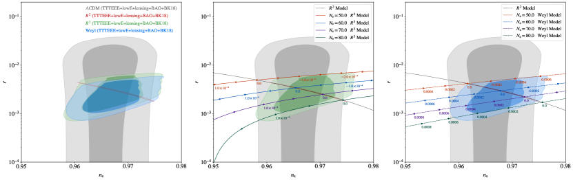
Figure 1: (left) Marginalized joint 68% and 95% CL regions for $n_{\rm s}$ and $r$ ($k_{*}=0.002$ Mpc^-1) for $\Lambda$CDM model (grey), Starobinsky $R^{2}$ model (red), Extended Starobinsky $R^{3}$ model (green) and Weyl model (blue) from Planck TTTEEE+lowE+lensing+BAO+BK18. (middle) Same as the left panel but focusing on the Starobinsky and the Extended Starobinsky model with plots of varying $N_{\rm e}$ for $R^{2}$ model (dotted) and ($N_{\rm e}$, $\delta$) for $R^{3}$ model (solid) superimposed. (right) Same as the left panel but focusing on the Starobinsky and the Weyl model with plots of varying $N_{\rm e}$ for $R^{2}$ model (dotted) and ($N_{\rm e}$, $\gamma_{\rm W}$) for Weyl model (dashed) superimposed.

6 Discussions and Conclusions

We shall begin our discussion section by addressing the common features shared by all models before providing a detailed discussion of each individual model. Additionally, we will offer comparison between different datasets. We also provide comments on the choice of $k_{*}$, $H_{0}$ and $S_{8}$ tension, and additional observational data that could further refine the constraints on the model. Finally, we offer a concluding summary at the end.

6.1 Common features

Overall, all the models are in good agreement with all observational data we employed, including both CMB and large-scale structure data, within a constrained range of parameters that are specific to each model. The common parameter to all the model is the $e$-folding number $N_{\rm e}$. Only $N_{\rm e}$ in the Starobinsky $R^{2}$ model could be constrained within a range of approximately $60-70$ (See Table 3 for example) consistent with predictions for other inflationary models (see, for example, Liddle et al. (1994), Liddle & Leach (2003), Groot Nibbelink & van Tent (2002)). For the other two models, the values of $N_{\rm e}$ could not be constrained within the range of our prior due to degeneracy with the other parameter ($\delta$ for $R^{3}$ Starobinsky model or $\gamma_{\rm W}$ for Weyl model). The Starobinsky $R^{2}$ model gives tightest constraints overall in comparison to the other models due to having less parameter. The values of $\delta$ and $\gamma_{\rm W}$ fall within $1\sigma$ from zero. From the datasets, it is suggested that the faster the inflation ends, the higher the tensor mode. This can be understood from the formulas for $n_{\rm s}$ and $r$ as decreasing functions of $N_{\rm e}$, as given in Eq. (27) and Eq. (2.2) for the $R^{3},R^{2}~{}(\delta=0)$ model and Eq. (41) and Eq. (42) for the Weyl model.

Our constraints on $N_{\rm e}$ for the Starobinsky $R^{2}$ model differ significantly from the one in Planck Collaboration et al. (2020a). Several reasons account for these discrepancies. The primary factor contributing to this difference is the choice of prior. In Planck Collaboration et al. (2020a), the prior is set to $[50,60]$, whereas in our work, it is extended to $[50,80]$. Another reason is the exact formula we use for $n_{\rm s}$ in Eq. (27) which contains higher order terms of $1/N_{\rm e}$, see Eq. (33) for approximation up to the order $N_{\rm e}^{-2}$. The inclusion of the higher order terms of $1/N_{\rm e}$ leads to a preference for a higher value of $n_{\rm s}$ from the data, as illustrated in the middle panel of Fig. 1.

For the cosmological parameters, there is good agreement with minor deviations among different models and datasets. The values of the spectral index $n_{\rm s}$ align with those of the standard $\Lambda$CDM. The tensor-to-scalar ratio $r$ can be constrained with both an upper and lower bound. However, the lower bound constraint on $r$ is purportedly influenced by our choice of prior on $N_{\rm e}$ which could go to zero as $N_{\rm e}\rightarrow\infty$ for the $R^{3}$ and Weyl model. The upper bound constraint on $r$ is also mildly effected by the choice on lower bound on prior of $N_{\rm e}$. We will elaborate this point further in Sec. 6.2 and Sec. 6.3. In addition, we find no strong evidence for the existence of running parameters within the models. However, our results show a preference for a negative value of $n_{\rm run}$ and positive value of $n_{\rm run,run}$ with a deviation within $1\sigma-2\sigma$. Regarding $n_{\rm t}$ and $n_{\rm t,run}$, our results also suggest a preference for a negative value within $1\sigma-2\sigma$.

Table 3: 95% CL parameter constraints on parameters specific to the models for $k_{*}=0.002,0.05\ {\rm Mpc}^{-1}$. $N_{\rm e}$ is the parameter common to all models; however, only $N_{\rm e}$ from $R^{2}$ model could be constrained from the datasets within the range defined by our prior.

	$R^{2}$ Model		$R^{3}$ Model		Weyl Model
Parameter	$N_{\rm e}$		$\delta\ (\times 10^{-4})$		$\gamma_{\rm W}\ (\times 10^{-4})$
$k_{*}$ (Mpc-1)	0.002	0.05	0.002	0.05	0.002	0.05
Planck	$64^{+10}_{-10}$	$62^{+10}_{-10}$	$-0.1^{+1.3}_{-1.4}$	$-0.1^{+1.1}_{-1.3}$	$1.1^{+4.5}_{-4.7}$	$1.6^{+4.0}_{-4.5}$
Planck+BK18	$63^{+10}_{-10}$	$60^{+10}_{-10}$	$0.0^{+1.2}_{-1.4}$	$0.2^{+1.1}_{-1.3}$	$1.1^{+4.4}_{-4.9}$	$1.6^{+4.0}_{-4.5}$
Planck+BAO	$67^{+10}_{-10}$	$64^{+10}_{-10}$	$-0.2^{+1.2}_{-1.4}$	$-0.1^{+1.0}_{-1.2}$	$0.4^{+4.2}_{-4.8}$	$1.0^{+3.9}_{-4.2}$
Planck+DES	$70^{+10}_{-10}$	$67^{+10}_{-10}$	$-0.4^{+1.2}_{-1.4}$	$-0.3^{+1.1}_{-1.3}$	$-0.1^{+4.3}_{-4.8}$	$0.5^{+4.0}_{-4.4}$
Planck+Pantheon+	$65^{+10}_{-10}$	$63^{+10}_{-10}$	$-0.2^{+1.2}_{-1.4}$	$0.0^{+1.1}_{-1.3}$	$0.7^{+4.3}_{-5.0}$	$1.3^{+3.8}_{-4.4}$
Planck+BAO+BK18	$66^{+10}_{-10}$	$63^{+10}_{-10}$	$-0.2^{+1.2}_{-1.4}$	$-0.2^{+1.1}_{-1.2}$	$0.2^{+4.3}_{-4.7}$	$0.9^{+3.7}_{-4.2}$
Planck+BAO+DES	$70^{+10}_{-10}$	$67^{+10}_{-10}$	$-0.4^{+1.2}_{-1.5}$	$0.0^{+1.1}_{-1.2}$	$-0.1^{+3.9}_{-4.9}$	$0.4^{+3.6}_{-4.3}$

6.2 $R^{2}$ Model and $R^{3}$ Model

The primary distinction between the Starobinsky $R^{2}$ model and the extended Starobinsky $R^{3}$ model lies in the value of the $\delta$ parameter in Eqs. (27)–(32). The Starobinsky $R^{2}$ model is obtained by setting $\delta=0$ within the extended $R^{3}$ model. For the $R^{3}$ model, the value of $\delta$ is close to zero and falls within the range of $-2\times 10^{-4}<\delta<1\times 10^{-4}$. However, the probability density function (pdf) is negatively skewed to the left, indicating a preference for negative values. The negative values of $\delta$ would suggest a preference for higher values of $n_{\rm s}$ and $r$ as shown in Fig. 1 as well as lower value of $N_{\rm e}$.

Fig. 3 displays the marginalized posterior probability distribution for the main parameters, while Fig. 9 presents the same plot for the power spectrum parameters of the Starobinsky $R^{2}$ model. Similarly Fig. 4 and Fig. 10 displays the same plot for the extended Starobinsky $R^{3}$ model. Our results are in good agreement with Cheong et al. (2020). The power spectrum parameters $n_{\rm s}$, $r$, $n_{\rm run}$, $n_{\rm run,run}$, $n_{\rm t}$ and $n_{\rm t,run}$ in $R^{2}$ Starobinsky model are strongly correlated to one another due to explicit relations in Eqs. (27)–(32). Nevertheless, the correlations of the power spectrum in the $R^{3}$ Starobinsky model are less pronounced, mainly because of the influence of the $\delta$ parameter.

Another reason for the unconstrained nature of $N_{\rm e}$ for $R^{3}$ model, in addition to the presence of the additional parameter $\delta$ as mentioned in the aformentioned section, is that in the limit $N_{\rm e}\rightarrow\infty$, the model constraint would converge to $r\rightarrow 0$ (see Eq. (34)) while $n_{s}$ could still lie within the constraints from observations. This renders the model dependent on the prior of $N_{\rm e}$ and $\delta$. Hence, an independent prior on $N_{\rm e}$ is crucial for constraining the $R^{3}$ model.

6.3 Weyl Model

The Weyl model differs from the Starobinsky model in its origin by incorporating an additional scalar field instead of additional terms in the geometrical part in the gravity action. However, the Weyl model exhibits many features that are similar to the Starobinsky model, especially the $R^{3}$ model. For example, the dependence on an additional parameter apart from $N_{\rm e}$, leading to constraints on the power spectrum that are less pronounced than those of the $R^{2}$ model. The constraining power on the parameters from the Weyl model is also similar to that of the $R^{3}$ model (also $R^{2}$ model for the main cosmological parameters), as explicitly seen in Fig. 1. The Weyl model also inherits an unconstrained nature in $N_{\rm e}$–though not as explicitly as the $R^{3}$ model–due to its dependence on $N_{\rm e}$ through the function $\Theta$. However, as $N_{\rm e}\rightarrow\infty$, the Weyl model tends to prefer $r\rightarrow 0$ and a higher value of $n_{\rm s}$, similar to the $R^{3}$ model. The value of $\gamma_{\rm W}$ is also very close to zero and lies within the range $-5\times 10^{-4}<\gamma_{\rm W}<5\times 10^{-4}$ as shown in Table 3. The posterior probability density function of $\gamma_{\rm W}$ is slightly positively skewed, indicating preference on positive values as well as higher value of $N_{\rm e}$ and lower value of $n_{\rm s}$ and $r$.

6.4 Comparison between datasets

We conducted assessments of our models, utilizing data from CMB sources (Planck, BK18) and large-scale structure datasets (BAO, Pantheon+, DES), covering various cosmological parameters. Planck served as the foundational dataset, supplemented with additional data (See Table 2). Therefore, the main constraining power typically arises from the Planck CMB data. In general, the constraints on cosmological parameters are similar to one another but exhibit some consistent deviations between datasets. For example, the CMB data (Planck and BK18) consistently favours lower values of $\Omega_{\rm b}h^{2}$ than the large-scale data, whereas the opposite is true for $\Omega_{\rm c}h^{2}$ as can been seen from Table 4 - 7. From the tables, the values of $\theta_{\rm MC}$ and $\tau$ also consistently increase across different datasets, from CMB to large-scale structure data while the opposite is true for $A_{\rm s}$. Regarding the power spectrum parameters, there is a tendency for the values of $n_{\rm s}$ to increase from CMB data to large-scale data as can be observed from Table 8 - 11. In general, the variation in the constraints on cosmological parameters consistently differs between the CMB data (Planck, BK18) and large-scale structure data (BAO, Pantheon+, DES). The extreme constraints from the CMB data are from BAO+BK18 or BK18, while the other extreme arises from DES or BAO+DES.

6.5 Effects of $k_{*}$ on Cosmological Parameters

In this work, the two choices of $k_{*}$; $k_{*}=0.002\ {\rm Mpc}^{-1}$ and $k_{*}=0.05\ {\rm Mpc}^{-1}$, are used as benchmarks in our work for the purpose of comparison with existing literature (for example, Planck Collaboration et al. (2020a, c)). The choice of $k_{*}$ is arbitrary; however, it is often based on practical considerations and the goal of capturing relevant information specific to a model or dataset. Our results show no notable distinction in the constraints on cosmological parameters between the two choices of $k_{*}$ except for $N_{\rm e}$, $\delta$, $\gamma_{\rm W}$ and $A_{\rm s}$. It is worth noting, as shown in Table 3, that the mean value of $N_{\rm e}$ differs by 2–3 between the two choices of $k_{*}$. Typically, $k_{*}=0.002\ {\rm Mpc}^{-1}$ favours lower values of $\delta$ and $\gamma_{\rm W}$ in comparison to $k_{*}=0.05\ {\rm Mpc}^{-1}$.

Referring to Eq. (25), for the scalar power spectrum amplitude $A_{\rm s}$, the values of $\ln A_{s}$ at two different $k_{*}$ values are well approximated by

$$\ln\Big{(}A_{\rm s}\;\big{|}_{k_{*}=\rm 0.002\ Mpc^{-1}}\Big{)} \approx \ln\Big{(}A_{\rm s}\;\big{|}_{k_{*}=\rm 0.05\ Mpc^{-1}}\Big{)}$$ (47)

$$+\ln 25\times(1-n_{\rm s}),$$

where $A_{\rm s}\;\big{|}_{k_{*}=\rm 0.002\ Mpc^{-1}}$ and $A_{\rm s}\;\big{|}_{k_{*}=\rm 0.05\ Mpc^{-1}}$ are the scalar amplitude at $k_{*}=0.002\ {\rm Mpc}^{-1}$ and $k_{*}=0.05\ {\rm Mpc}^{-1}$ respectively.

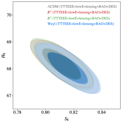
Figure 2: Marginalized joint 68% and 95% CL regions for $H_{0}$ and $S_{8}$ ($k_{*}=0.05$ Mpc^-1) for Planck+BAO+DES between different models.

6.6 $H_{0}$ and $S_{8}$ Tensions

The Hubble tension stands out as one of the most statistically significant discrepancies in observational cosmology, showing a disagreement of 4$\sigma$ to 6$\sigma$ between early-time and late-time observations (See Di Valentino et al. (2021) and references therein). For example, a late-time measurement of $H_{0}$ from Pantheon+SH0ES yields $H_{0}=73.04\pm 1.04\ {\rm km\ s}^{-1}\ {\rm Mpc}^{-1}$ (Riess et al., 2022), while an early-time measurement from Planck CMB gives $H_{0}=67.4\pm 0.5\ {\rm km\ s}^{-1}\ {\rm Mpc}^{-1}$ (Planck Collaboration et al., 2020c). The discrepancy between these two measurements is approximately $5.5\sigma$.

Another tension related to the inconsistency between early-time and late-time measurements involves $\sigma_{8}$, which represents the amplitude of the power spectrum at a scale of 8 Mpc. This tension is commonly expressed in terms of $S_{8}$ ($\sigma_{8}(\Omega_{\rm m}/0.3)^{0.5}$), influencing the amplitude of weak lensing measurements. The measurements from lower redshift probes systematically favour lower value of $S_{8}$ compared to those obtained from high-redshift CMB measurements (Abdalla et al., 2022). For instance, an early-time measurement from Planck CMB gives $S_{8}=0.834\pm 0.016$ (Planck Collaboration et al., 2020c), while a late-time measurement from DES weak gravitational lensing yields $S_{8}=0.759\pm 0.025$ (Amon et al., 2022).

When comparing constraints across different datasets, we observe that the Planck+DES and Planck+BAO+DES datasets systematically favour a lower value of $S_{8}$ and a higher value of $H_{0}$. For example, the constraints on $(S_{8},H_{0})$ for $R^{2}$ model are $(0.812^{+0.018}_{-0.018},68.19^{+0.72}_{-0.72})$ for Planck+BAO+DES, while Planck alone gives $(0.830^{+0.024}_{-0.024},67.50^{+1.00}_{-0.99})$. When comparing between different models, our findings indicate that, with the exception of Planck + DES and Planck + BAO + DES dataset, the constraints on $S_{8}$ and $H_{0}$ remain consistent across all datasets and all models. Fig. 2 displays marginalized joint 68% and 95% confidence level regions for $S_{8}$ and $H_{0}$ ($k_{*}=0.05$ Mpc^-1) for Planck+DES amongst different models. In terms of mean values, the Starobinsky models exhibit a tendency toward lower values of $S_{8}$ and higher values of $H_{0}$ compared to the $\Lambda$CDM and Weyl model. Our results continue to highlight tension between Planck CMB measurements and late-time observations, particularly with respect to the DES dataset.

6.7 Future Observational Constraints

In the forthcoming years, we would be able to evaluate inflationary predictions through direct measurements of the tensor power spectrum. This will primarily involve detecting B-mode polarization arising from gravitational waves generated during inflation, commonly known as primordial gravitational waves. The significance of detecting primordial gravitational waves cannot be overemphasized, as they hold important information about the physics of the very early Universe. Confirming the inflationary scenarios becomes pivotal, as the detection of the tensor-to-scalar ratio $r$ can be directly inferred the energy scale of inflation (Lyth & Riotto, 1999). This assessment will encompass both current and upcoming experiments. For a comprehensive overview of experiments targeting the measurement of primordial gravitational waves, we suggest Campeti et al. (2021).

According to Fig. 1, the absence of detection of $r$ above 0.001 would possibly lead to exclusion of the Starobinsky $R^{2}$ model and impose stringent constraints on the Starobinsky $R^{3}$ model and Weyl model; hence, we shall discuss experiments that could potentially provide stringent constraints or a definitive rejection of the models in the next decade. For example, the Lite (Light) satellite for the study of B-mode polarization and inflation from cosmic background Radiation Detection (LiteBIRD) (LiteBIRD Collaboration et al., 2023) is a space-based experiment which will study the B-mode polarization from CMB. It aims to establish a lower limit on the tensor-to-scalar ratio. The expected sensitivity for LiteBIRD on tensor-to-scalar ratio is $r<0.003$ at 95% confidence level for a fiducial model with $r=0$. Tighter constraints are anticipated when combining LiteBIRD data with that from other experiments (Crowder & Cornish, 2005). Similarly, Simons Observatory (SO), which is a ground-based CMB experiment, is also anticipated to give $r<0.003$ at 95% confidence level for a fiducial model with $r=0$ (Ade et al., 2019).

Looking far into the coming decades, planned space-based experiments include the DECi-hertz Interferometer Gravitational wave Observatory (DECIGO) (Seto et al., 2001; Kuroyanagi et al., 2015), Big Bang Observer (BBO) (Crowder & Cornish, 2005), $\mu$ARES (Sesana et al., 2021) which are laser interferometers similar to Laser Interferometer Space Antenna (LISA) (Bartolo et al., 2016). Those proposed experiments aim to push the constraint on $r$ to the cosmic variance limit, achieving $r<10^{-4}$ for a fiducial model with $r=0$.

Here is the summary of our results.

• We consider three different inflationary models from different theories of gravitation; Starobinsky $R^{2}$, extended Starobinsky $R^{3}$ and Weyl model by considering scalar perturbations and tensor perturbations parameterized by power-law forms in Eq. (25) and Eq. (26). The constraints on cosmological parameters, derived using the dataset in Table 1, indicate that all models are in good agreement with the observational data.

• Only $N_{\rm e}$ in the Starobinsky $R^{2}$ model could be constrained giving the mean value of $N_{\rm e}$ approximately 60–70 consistent with predictions from other inflation models (See Table 3).

• While the Weyl model differs from the extended Starobinsky $R^{3}$ model in its origin, the observational constraints on both models are very similar. Hence, distinguishing between the models would require independent observations. However, with current datasets that cannot exclude very small tensor-to-scalar ratio $r<0.001$ region, there is no compelling evidence supporting the preference of the $R^{3}$ model and the Weyl model over the $R^{2}$ Starobinsky model. Future observations would allow us to distinguish the $R^{2}$ model from the $R^{3}$ and Weyl model with the probe in $r<0.001$ region of the parameter space.

• We investigate the effect of the choice of $k_{*}$ that are frequently used in literature and find that $k_{*}=0.002\ {\rm Mpc}^{-1}$ favours lower value of $\delta$ and $\gamma_{\rm W}$ compared to $k_{*}=0.05\ {\rm Mpc}^{-1}$. For all models, larger $k_{*}$ results in smaller constrained value of $A_{s}$. In addition, the mean value of $N_{\rm e}$ differs by 2–3 between the two choices of $k_{*}$’s.

• Our results continue to emphasize the tension in $H_{0}$ and $S_{8}$ between early-time CMB measurements and late-time large-scale structure observations.

We would like to thank Utane Sawangwit and the National Astronomical Research Institute of Thailand (NARIT) for facilitating the Chalawan HPC and thank greatly the NSTDA Supercomputer center (ThaiSC) and the National e-Science Infrastructure Consortium for their support of computing facilities used in this work. PB and PB are supported in part by National Research Council of Thailand (NRCT) and Chulalongkorn University under Grant N42A660500. This research has received funding support from the NSRF via the Program Management Unit for Human Resources & Institutional Development, Research and Innovation [grant number B39G660025]. TC is supported by Naresuan University (NU), and the National Science, Research and Innovation Fund (NSRF) Grant number R2566B091.

In this section, we shall provide all the tables and figures displaying the constraints on relevant parameters. For detailed explanations and discussions, the reader should refer to the main text in Sec. 5 and Sec. 6.

Appendix A Parameter Constraints

A.1 Main parameters

We provide constraints on the main cosmological parameter that are relevant to our work. The standard parameters are $\Omega_{\rm b}h^{2}$, $\Omega_{\rm c}h^{2}$, $\theta_{\rm MC}$, $\tau$, ${\rm ln}(10^{10}A_{\rm s})$. We also include $H_{0}$ and $S_{8}$ in the parameter set as a reference to the discussion on $H_{0}$ and $S_{8}$ tension in Sec. 6.6.

	$R^{2}$ Model	$R^{3}$ Model	Weyl Model	$\Lambda$CDM
Parameter	95% limits	95% limits	95% limits	95% limits
$\Omega_{\rm b}h^{2}$	$0.02239^{+0.00028}_{-0.00028}$	$0.02238^{+0.00028}_{-0.00028}$	$0.02237^{+0.00029}_{-0.00029}$	$0.02238^{+0.00030}_{-0.00029}$
	$0.02239^{+0.00028}_{-0.00028}$	$0.02238^{+0.00029}_{-0.00028}$	$0.02237^{+0.00030}_{-0.00028}$	$0.02238^{+0.00029}_{-0.00029}$
$\Omega_{\rm c}h^{2}$	$0.1199^{+0.0023}_{-0.0022}$	$0.1200^{+0.0023}_{-0.0023}$	$0.1200^{+0.0024}_{-0.0024}$	$0.1199^{+0.0024}_{-0.0023}$
	$0.1198^{+0.0022}_{-0.0022}$	$0.1200^{+0.0023}_{-0.0024}$	$0.1201^{+0.0023}_{-0.0023}$	$0.1199^{+0.0024}_{-0.0024}$
$100\theta_{\rm MC}$	$1.04092^{+0.00059}_{-0.00059}$	$1.04092^{+0.00061}_{-0.00060}$	$1.04091^{+0.00060}_{-0.00061}$	$1.04092^{+0.00062}_{-0.00061}$
	$1.04094^{+0.00059}_{-0.00060}$	$1.04092^{+0.00060}_{-0.00061}$	$1.04090^{+0.00060}_{-0.00059}$	$1.04091^{+0.00060}_{-0.00062}$
$\tau$	$0.055^{+0.015}_{-0.014}$	$0.054^{+0.015}_{-0.015}$	$0.054^{+0.016}_{-0.015}$	$0.055^{+0.015}_{-0.014}$
	$0.055^{+0.015}_{-0.014}$	$0.055^{+0.015}_{-0.014}$	$0.055^{+0.015}_{-0.014}$	$0.055^{+0.015}_{-0.015}$
${\rm{ln}}(10^{10}A_{\rm s})$	$3.155^{+0.032}_{-0.032}$	$3.155^{+0.034}_{-0.033}$	$3.156^{+0.033}_{-0.034}$	$3.155^{+0.033}_{-0.033}$
	$3.046^{+0.029}_{-0.028}$	$3.045^{+0.029}_{-0.028}$	$3.045^{+0.029}_{-0.028}$	$3.045^{+0.030}_{-0.028}$
$H_{0}$	$67.40^{+0.99}_{-1.0}$	$67.4^{+1.1}_{-1.0}$	$67.3^{+1.1}_{-1.1}$	$67.4^{+1.1}_{-1.1}$
	$67.5^{+1.0}_{-0.99}$	$67.4^{+1.1}_{-1.0}$	$67.3^{+1.1}_{-1.0}$	$67.4^{+1.1}_{-1.1}$
$S_{8}$	$0.831^{+0.024}_{-0.024}$	$0.831^{+0.025}_{-0.025}$	$0.832^{+0.026}_{-0.025}$	$0.831^{+0.026}_{-0.026}$
	$0.830^{+0.024}_{-0.024}$	$0.831^{+0.025}_{-0.025}$	$0.832^{+0.025}_{-0.025}$	$0.831^{+0.025}_{-0.025}$

Table 4: 95% Confidence limits of the main cosmological parameters for Planck TTTEEE+lowE+lensing dataset. The upper set of figures for each parameter are constraints at $k_{*}=0.002\ {\rm Mpc}^{-1}$ and the lower set of figures are constraints at $k_{*}=0.05\ {\rm Mpc}^{-1}$.

	$R^{2}$ Model	$R^{3}$ Model	Weyl Model	$\Lambda$CDM
Parameter	95% limits	95% limits	95% limits	95% limits
$\Omega_{\rm b}h^{2}$	$0.02241^{+0.00028}_{-0.00027}$	$0.02241^{+0.00029}_{-0.00028}$	$0.02240^{+0.00029}_{-0.00030}$	$0.02241^{+0.00028}_{-0.00028}$
	$0.02242^{+0.00029}_{-0.00027}$	$0.02241^{+0.00029}_{-0.00028}$	$0.02240^{+0.00028}_{-0.00028}$	$0.02241^{+0.00029}_{-0.00027}$
$\Omega_{\rm c}h^{2}$	$0.1196^{+0.0023}_{-0.0022}$	$0.1196^{+0.0024}_{-0.0024}$	$0.1197^{+0.0023}_{-0.0023}$	$0.1195^{+0.0024}_{-0.0024}$
	$0.1195^{+0.0022}_{-0.0022}$	$0.1196^{+0.0024}_{-0.0023}$	$0.1197^{+0.0023}_{-0.0023}$	$0.1195^{+0.0024}_{-0.0024}$
$100\theta_{\rm MC}$	$1.04097^{+0.00060}_{-0.00060}$	$1.04095^{+0.00060}_{-0.00060}$	$1.04096^{+0.00059}_{-0.00063}$	$1.04097^{+0.00062}_{-0.00062}$
	$1.04098^{+0.00059}_{-0.00059}$	$1.04095^{+0.00060}_{-0.00060}$	$1.04095^{+0.00059}_{-0.00060}$	$1.04097^{+0.00061}_{-0.00062}$
$\tau$	$0.056^{+0.015}_{-0.014}$	$0.056^{+0.016}_{-0.014}$	$0.056^{+0.015}_{-0.014}$	$0.056^{+0.016}_{-0.015}$
	$0.056^{+0.015}_{-0.014}$	$0.055^{+0.015}_{-0.015}$	$0.056^{+0.015}_{-0.014}$	$0.056^{+0.015}_{-0.014}$
${\rm{ln}}(10^{10}A_{\rm s})$	$3.153^{+0.032}_{-0.031}$	$3.154^{+0.033}_{-0.034}$	$3.155^{+0.034}_{-0.033}$	$3.153^{+0.033}_{-0.033}$
	$3.047^{+0.029}_{-0.028}$	$3.046^{+0.029}_{-0.028}$	$3.046^{+0.029}_{-0.027}$	$3.046^{+0.029}_{-0.028}$
$H_{0}$	$67.55^{+0.98}_{-1.0}$	$67.5^{+1.1}_{-1.0}$	$67.5^{+1.0}_{-1.0}$	$67.6^{+1.1}_{-1.1}$
	$67.60^{+0.99}_{-0.99}$	$67.5^{+1.1}_{-1.1}$	$67.5^{+1.1}_{-1.0}$	$67.6^{+1.1}_{-1.1}$
$S_{8}$	$0.828^{+0.025}_{-0.024}$	$0.829^{+0.025}_{-0.025}$	$0.829^{+0.024}_{-0.025}$	$0.827^{+0.026}_{-0.025}$
	$0.827^{+0.024}_{-0.024}$	$0.828^{+0.025}_{-0.025}$	$0.829^{+0.025}_{-0.024}$	$0.827^{+0.026}_{-0.026}$

Table 5: Same as Table 4 but for Planck TTTEEE+lowE+lensing+Pantheon+ dataset.

	$R^{2}$ Model	$R^{3}$ Model	Weyl Model	$\Lambda$CDM
Parameter	95% limits	95% limits	95% limits	95% limits
$\Omega_{\rm b}h^{2}$	$0.02242^{+0.00026}_{-0.00026}$	$0.02242^{+0.00026}_{-0.00026}$	$0.02241^{+0.00027}_{-0.00027}$	$0.02242^{+0.00027}_{-0.00026}$
	$0.02242^{+0.00026}_{-0.00026}$	$0.02242^{+0.00026}_{-0.00026}$	$0.02242^{+0.00026}_{-0.00026}$	$0.02242^{+0.00027}_{-0.00027}$
$\Omega_{\rm c}h^{2}$	$0.1194^{+0.0018}_{-0.0017}$	$0.1195^{+0.0019}_{-0.0018}$	$0.1195^{+0.0018}_{-0.0019}$	$0.1193^{+0.0018}_{-0.0018}$
	$0.1194^{+0.0018}_{-0.0018}$	$0.1194^{+0.0018}_{-0.0018}$	$0.1194^{+0.0019}_{-0.0018}$	$0.1193^{+0.0019}_{-0.0019}$
$100\theta_{\rm MC}$	$1.04100^{+0.00056}_{-0.00058}$	$1.04100^{+0.00057}_{-0.00057}$	$1.04100^{+0.00058}_{-0.00057}$	$1.04101^{+0.00058}_{-0.00058}$
	$1.04100^{+0.00057}_{-0.00057}$	$1.04100^{+0.00058}_{-0.00056}$	$1.04099^{+0.00056}_{-0.00058}$	$1.04100^{+0.00058}_{-0.00057}$
$\tau$	$0.057^{+0.014}_{-0.014}$	$0.057^{+0.015}_{-0.014}$	$0.057^{+0.015}_{-0.014}$	$0.057^{+0.015}_{-0.014}$
	$0.058^{+0.015}_{-0.014}$	$0.057^{+0.014}_{-0.014}$	$0.057^{+0.015}_{-0.014}$	$0.057^{+0.015}_{-0.014}$
${\rm{ln}}(10^{10}A_{\rm s})$	$3.155^{+0.031}_{-0.030}$	$3.156^{+0.033}_{-0.033}$	$3.156^{+0.033}_{-0.033}$	$3.155^{+0.032}_{-0.032}$
	$3.050^{+0.028}_{-0.027}$	$3.050^{+0.028}_{-0.027}$	$3.050^{+0.029}_{-0.027}$	$3.049^{+0.029}_{-0.028}$
$H_{0}$	$67.63^{+0.79}_{-0.81}$	$67.61^{+0.83}_{-0.82}$	$67.60^{+0.86}_{-0.81}$	$67.66^{+0.84}_{-0.81}$
	$67.65^{+0.80}_{-0.82}$	$67.62^{+0.83}_{-0.82}$	$67.62^{+0.84}_{-0.82}$	$67.66^{+0.85}_{-0.83}$
$S_{8}$	$0.827^{+0.020}_{-0.020}$	$0.828^{+0.020}_{-0.020}$	$0.828^{+0.020}_{-0.020}$	$0.826^{+0.020}_{-0.020}$
	$0.827^{+0.020}_{-0.020}$	$0.828^{+0.020}_{-0.020}$	$0.827^{+0.020}_{-0.020}$	$0.826^{+0.021}_{-0.021}$

Table 6: Same as Table 4 but for Planck TTTEEE+lowE+lensing+BAO+BK18 dataset.

	$R^{2}$ Model	$R^{3}$ Model	Weyl Model	$\Lambda$CDM
Parameter	95% limits	95% limits	95% limits	95% limits
$\Omega_{\rm b}h^{2}$	$0.02249^{+0.00025}_{-0.00025}$	$0.02250^{+0.00026}_{-0.00026}$	$0.02250^{+0.00026}_{-0.00026}$	$0.02249^{+0.00026}_{-0.00026}$
	$0.02252^{+0.00026}_{-0.00025}$	$0.02252^{+0.00026}_{-0.00026}$	$0.02249^{+0.00025}_{-0.00026}$	$0.02249^{+0.00026}_{-0.00026}$
$\Omega_{\rm c}h^{2}$	$0.1185^{+0.0016}_{-0.0015}$	$0.1185^{+0.0017}_{-0.0017}$	$0.1185^{+0.0017}_{-0.0017}$	$0.1184^{+0.0017}_{-0.0017}$
	$0.1182^{+0.0016}_{-0.0015}$	$0.1182^{+0.0017}_{-0.0017}$	$0.1185^{+0.0017}_{-0.0017}$	$0.1184^{+0.0017}_{-0.0017}$
$100\theta_{\rm MC}$	$1.04107^{+0.00057}_{-0.00058}$	$1.04108^{+0.00056}_{-0.00058}$	$1.04108^{+0.00056}_{-0.00057}$	$1.04108^{+0.00055}_{-0.00057}$
	$1.04109^{+0.00056}_{-0.00057}$	$1.04110^{+0.00056}_{-0.00057}$	$1.04107^{+0.00058}_{-0.00056}$	$1.04108^{+0.00057}_{-0.00056}$
$\tau$	$0.057^{+0.014}_{-0.014}$	$0.057^{+0.015}_{-0.014}$	$0.057^{+0.015}_{-0.014}$	$0.057^{+0.015}_{-0.014}$
	$0.057^{+0.015}_{-0.014}$	$0.057^{+0.015}_{-0.014}$	$0.057^{+0.016}_{-0.014}$	$0.057^{+0.015}_{-0.014}$
${\rm{ln}}(10^{10}A_{\rm s})$	$3.147^{+0.031}_{-0.030}$	$3.147^{+0.032}_{-0.031}$	$3.148^{+0.033}_{-0.031}$	$3.146^{+0.033}_{-0.033}$
	$3.046^{+0.029}_{-0.027}$	$3.046^{+0.029}_{-0.028}$	$3.047^{+0.030}_{-0.028}$	$3.047^{+0.029}_{-0.028}$
$H_{0}$	$68.02^{+0.71}_{-0.74}$	$68.04^{+0.76}_{-0.76}$	$68.04^{+0.77}_{-0.76}$	$68.05^{+0.78}_{-0.77}$
	$68.19^{+0.72}_{-0.72}$	$68.18^{+0.77}_{-0.76}$	$68.02^{+0.76}_{-0.76}$	$68.07^{+0.79}_{-0.76}$
$S_{8}$	$0.816^{+0.018}_{-0.018}$	$0.816^{+0.018}_{-0.018}$	$0.816^{+0.018}_{-0.018}$	$0.815^{+0.019}_{-0.018}$
	$0.812^{+0.018}_{-0.018}$	$0.812^{+0.018}_{-0.018}$	$0.816^{+0.019}_{-0.018}$	$0.815^{+0.019}_{-0.018}$

Table 7: Same as Table 4 but for Planck TTTEEE+lowE+lensing+BAO+DES dataset.

A.2 Power spectrum parameters

We summarize the constraints on the inflationary parameters in this section with $k_{*}=0.002,0.05\ {\rm Mpc}^{-1}$. The parameters are $n_{\rm s}$, $r$, $n_{\rm run}$, $n_{\rm run,run}$, $n_{\rm t}$ and $n_{\rm t,run}$

	$R^{2}$ Model	$R^{3}$ Model	Weyl Model	$\Lambda$CDM
Parameter	95% limits	95% limits	95% limits	95% limits
$n_{\rm s}$	$0.9671^{+0.0063}_{-0.0068}$	$0.9668^{+0.0088}_{-0.0086}$	$0.9661^{+0.0089}_{-0.0082}$	$0.9660^{+0.0080}_{-0.0084}$
	$0.9660^{+0.0070}_{-0.0068}$	$0.9651^{+0.0081}_{-0.0080}$	$0.9648^{+0.0080}_{-0.0079}$	$0.9658^{+0.0084}_{-0.0083}$
$r$	$0.0031^{+0.0012}_{-0.0011}$	$0.0034^{+0.0027}_{-0.0023}$	$0.0026^{+0.0021}_{-0.0017}$	$<0.115$
	$0.0033^{+0.0014}_{-0.0012}$	$0.0031^{+0.0026}_{-0.0022}$	$0.0024^{+0.0020}_{-0.0015}$	$<0.117$
$n_{\rm run}$	$-0.00055^{+0.00020}_{-0.00023}$	$-0.00060^{+0.00040}_{-0.00048}$	$-0.00045^{+0.00030}_{-0.00037}$
	$-0.00059^{+0.00022}_{-0.00025}$	$-0.00056^{+0.00038}_{-0.00045}$	$-0.00043^{+0.00027}_{-0.00036}$
$n_{\rm run,run}$	$\left(\,1.9^{+1.2}_{-1.0}\,\right)\cdot 10^{-5}$	$\left(\,2.0^{+1.5}_{-1.2}\,\right)\cdot 10^{-5}$	$\left(\,1.52^{+1.2}_{-0.88}\,\right)\cdot 10^{-5}$
	$\left(\,2.1^{+1.3}_{-1.1}\,\right)\cdot 10^{-5}$	$\left(\,2.0^{+1.7}_{-1.2}\,\right)\cdot 10^{-5}$	$\left(\,1.51^{+1.2}_{-0.87}\,\right)\cdot 10^{-5}$
$n_{\rm t}$	$-0.00039^{+0.00014}_{-0.00015}$	$-0.00042^{+0.00029}_{-0.00034}$	$-0.00032^{+0.00021}_{-0.00027}$
	$-0.00042^{+0.00015}_{-0.00017}$	$-0.00039^{+0.00027}_{-0.00032}$	$-0.00030^{+0.00019}_{-0.00025}$
$n_{\rm t,run}$	$\left(\,-13.0^{+6.7}_{-7.9}\,\right)\cdot 10^{-6}$	$\left(\,-14.0^{+7.9}_{-10}\,\right)\cdot 10^{-6}$	$\left(\,-10.4^{+6.0}_{-7.8}\,\right)\cdot 10^{-6}$
	$\left(\,-14.3^{+7.5}_{-8.6}\,\right)\cdot 10^{-6}$	$\left(\,-13.8^{+7.7}_{-11}\,\right)\cdot 10^{-6}$	$\left(\,-10.4^{+5.9}_{-8.0}\,\right)\cdot 10^{-6}$

Table 8: 95% Confidence limits of the power spectrum parameters for Planck TTTEEE+lowE+lensing dataset. The upper set of figures for each parameter are constraints at $k_{*}=0.002\ {\rm Mpc}^{-1}$ and the lower set of figures are constraints at $k_{*}=0.05\ {\rm Mpc}^{-1}$.

	$R^{2}$ Model	$R^{3}$ Model	Weyl Model	$\Lambda$CDM
Parameter	95% limits	95% limits	95% limits	95% limits
$n_{\rm s}$	$0.9678^{+0.0060}_{-0.0063}$	$0.9677^{+0.0087}_{-0.0084}$	$0.9670^{+0.0087}_{-0.0083}$	$0.9671^{+0.0083}_{-0.0085}$
	$0.9666^{+0.0067}_{-0.0070}$	$0.9660^{+0.0079}_{-0.0080}$	$0.9656^{+0.0080}_{-0.0078}$	$0.9668^{+0.0084}_{-0.0081}$
$r$	$0.0030^{+0.0012}_{-0.0010}$	$0.0034^{+0.0027}_{-0.0023}$	$0.0026^{+0.0022}_{-0.0017}$	$<0.113$
	$0.0032^{+0.0013}_{-0.0012}$	$0.0032^{+0.0027}_{-0.0022}$	$0.0025^{+0.0020}_{-0.0016}$	$<0.125$
$n_{\rm run}$	$-0.00053^{+0.00019}_{-0.00021}$	$-0.00060^{+0.00039}_{-0.00047}$	$-0.00047^{+0.00030}_{-0.00039}$
	$-0.00057^{+0.00022}_{-0.00024}$	$-0.00056^{+0.00038}_{-0.00047}$	$-0.00044^{+0.00028}_{-0.00036}$
$n_{\rm run,run}$	$\left(\,1.76^{+1.1}_{-0.90}\,\right)\cdot 10^{-5}$	$\left(\,2.0^{+1.5}_{-1.1}\,\right)\cdot 10^{-5}$	$\left(\,1.53^{+1.2}_{-0.86}\,\right)\cdot 10^{-5}$
	$\left(\,2.0^{+1.3}_{-1.1}\,\right)\cdot 10^{-5}$	$\left(\,2.0^{+1.7}_{-1.1}\,\right)\cdot 10^{-5}$	$\left(\,1.53^{+1.2}_{-0.87}\,\right)\cdot 10^{-5}$
$n_{\rm t}$	$-0.00037^{+0.00013}_{-0.00015}$	$-0.00042^{+0.00028}_{-0.00034}$	$-0.00033^{+0.00022}_{-0.00028}$
	$-0.00040^{+0.00015}_{-0.00016}$	$-0.00040^{+0.00027}_{-0.00034}$	$-0.00031^{+0.00020}_{-0.00025}$
$n_{\rm t,run}$	$\left(\,-12.1^{+6.1}_{-7.3}\,\right)\cdot 10^{-6}$	$\left(\,-13.6^{+7.6}_{-10}\,\right)\cdot 10^{-6}$	$\left(\,-10.5^{+5.9}_{-7.7}\,\right)\cdot 10^{-6}$
	$\left(\,-13.6^{+7.2}_{-8.4}\,\right)\cdot 10^{-6}$	$\left(\,-13.6^{+7.6}_{-11}\,\right)\cdot 10^{-6}$	$\left(\,-10.5^{+5.9}_{-7.9}\,\right)\cdot 10^{-6}$

Table 9: Same as Table 8 but for Planck TTTEEE+lowE+lensing+Pantheon+ dataset.

	$R^{2}$ Model	$R^{3}$ Model	Weyl Model	$\Lambda$CDM
Parameter	95% limits	95% limits	95% limits	95% limits
$n_{\rm s}$	$0.9682^{+0.0056}_{-0.0060}$	$0.9680^{+0.0077}_{-0.0078}$	$0.9679^{+0.0079}_{-0.0077}$	$0.9668^{+0.0072}_{-0.0072}$
	$0.9669^{+0.0063}_{-0.0068}$	$0.9663^{+0.0076}_{-0.0074}$	$0.9663^{+0.0072}_{-0.0071}$	$0.9668^{+0.0073}_{-0.0073}$
$r$	$0.00293^{+0.0011}_{-0.00098}$	$0.0034^{+0.0027}_{-0.0023}$	$0.0029^{+0.0022}_{-0.0018}$	$<0.0313$
	$0.0032^{+0.0012}_{-0.0011}$	$0.0032^{+0.0026}_{-0.0021}$	$0.0027^{+0.0020}_{-0.0017}$	$<0.0358$
$n_{\rm run}$	$-0.00052^{+0.00018}_{-0.00020}$	$-0.00060^{+0.00040}_{-0.00048}$	$-0.00050^{+0.00032}_{-0.00039}$
	$-0.00056^{+0.00021}_{-0.00023}$	$-0.00057^{+0.00037}_{-0.00045}$	$-0.00047^{+0.00029}_{-0.00036}$
$n_{\rm run,run}$	$\left(\,1.71^{+1.0}_{-0.84}\,\right)\cdot 10^{-5}$	$\left(\,2.0^{+1.7}_{-1.1}\,\right)\cdot 10^{-5}$	$\left(\,1.61^{+1.1}_{-0.91}\,\right)\cdot 10^{-5}$
	$\left(\,1.9^{+1.2}_{-1.0}\,\right)\cdot 10^{-5}$	$\left(\,2.0^{+1.7}_{-1.1}\,\right)\cdot 10^{-5}$	$\left(\,1.60^{+1.2}_{-0.91}\,\right)\cdot 10^{-5}$
$n_{\rm t}$	$-0.00037^{+0.00012}_{-0.00014}$	$-0.00043^{+0.00028}_{-0.00034}$	$-0.00036^{+0.00023}_{-0.00028}$
	$-0.00040^{+0.00014}_{-0.00016}$	$-0.00040^{+0.00027}_{-0.00032}$	$-0.00033^{+0.00021}_{-0.00025}$
$n_{\rm t,run}$	$\left(\,-11.7^{+5.6}_{-6.9}\,\right)\cdot 10^{-6}$	$\left(\,-13.7^{+7.6}_{-11}\,\right)\cdot 10^{-6}$	$\left(\,-11.0^{+6.2}_{-7.3}\,\right)\cdot 10^{-6}$
	$\left(\,-13.2^{+6.8}_{-8.0}\,\right)\cdot 10^{-6}$	$\left(\,-13.6^{+7.6}_{-11}\,\right)\cdot 10^{-6}$	$\left(\,-11.0^{+6.1}_{-7.7}\,\right)\cdot 10^{-6}$

Table 10: Same as Table 8 but for Planck TTTEEE+lowE+lensing+BAO+BK18 dataset.

	$R^{2}$ Model	$R^{3}$ Model	Weyl Model	$\Lambda$CDM
Parameter	95% limits	95% limits	95% limits	95% limits
$n_{\rm s}$	$0.9696^{+0.0047}_{-0.0054}$	$0.9700^{+0.0075}_{-0.0076}$	$0.9695^{+0.0075}_{-0.0074}$	$0.9690^{+0.0074}_{-0.0072}$
	$0.9688^{+0.0054}_{-0.0058}$	$0.9686^{+0.0071}_{-0.0071}$	$0.9680^{+0.0070}_{-0.0071}$	$0.9691^{+0.0073}_{-0.0073}$
$r$	$0.00268^{+0.00097}_{-0.00078}$	$0.0035^{+0.0028}_{-0.0023}$	$0.0028^{+0.0024}_{-0.0017}$	$<0.114$
	$0.00281^{+0.0011}_{-0.00090}$	$0.0034^{+0.0026}_{-0.0021}$	$0.0027^{+0.0021}_{-0.0016}$	$<0.132$
$n_{\rm run}$	$-0.00047^{+0.00014}_{-0.00018}$	$-0.00062^{+0.00039}_{-0.00050}$	$-0.00049^{+0.00030}_{-0.00041}$
	$-0.00050^{+0.00016}_{-0.00019}$	$-0.00060^{+0.00037}_{-0.00046}$	$-0.00047^{+0.00028}_{-0.00037}$
$n_{\rm run,run}$	$\left(\,1.49^{+0.86}_{-0.64}\,\right)\cdot 10^{-5}$	$\left(\,2.0^{+1.7}_{-1.1}\,\right)\cdot 10^{-5}$	$\left(\,1.49^{+1.1}_{-0.82}\,\right)\cdot 10^{-5}$
	$\left(\,1.60^{+0.97}_{-0.74}\,\right)\cdot 10^{-5}$	$\left(\,2.0^{+1.7}_{-1.1}\,\right)\cdot 10^{-5}$	$\left(\,1.53^{+1.2}_{-0.84}\,\right)\cdot 10^{-5}$
$n_{\rm t}$	$-0.000335^{+0.000098}_{-0.00012}$	$-0.00044^{+0.00028}_{-0.00035}$	$-0.00035^{+0.00022}_{-0.00029}$
	$-0.00035^{+0.00011}_{-0.00013}$	$-0.00043^{+0.00026}_{-0.00032}$	$-0.00034^{+0.00020}_{-0.00027}$
$n_{\rm t,run}$	$\left(\,-10.3^{+4.3}_{-5.8}\,\right)\cdot 10^{-6}$	$\left(\,-13.4^{+7.4}_{-11}\,\right)\cdot 10^{-6}$	$\left(\,-10.3^{+5.5}_{-7.5}\,\right)\cdot 10^{-6}$
	$\left(\,-11.0^{+5.0}_{-6.5}\,\right)\cdot 10^{-6}$	$\left(\,-13.5^{+7.5}_{-11}\,\right)\cdot 10^{-6}$	$\left(\,-10.5^{+5.7}_{-7.7}\,\right)\cdot 10^{-6}$

Table 11: Same as Table 8 but for Planck TTTEEE+lowE+lensing+BAO+DES dataset.

References

- Abbott et al. (2018) Abbott, T. M. C., Abdalla, F. B., Alarcon, A., et al. 2018, Phys. Rev. D, 98, 043526, doi: 10.1103/PhysRevD.98.043526
- Abdalla et al. (2022) Abdalla, E., Abellán, G. F., Aboubrahim, A., et al. 2022, Journal of High Energy Astrophysics, 34, 49, doi: 10.1016/j.jheap.2022.04.002
- Ade et al. (2019) Ade, P., Aguirre, J., Ahmed, Z., et al. 2019, J. Cosmology Astropart. Phys, 2019, 056, doi: 10.1088/1475-7516/2019/02/056
- Ade et al. (2021) Ade, P. A. R., Ahmed, Z., Amiri, M., et al. 2021, Phys. Rev. Lett., 127, 151301, doi: 10.1103/PhysRevLett.127.151301
- Alam et al. (2017) Alam, S., Ata, M., Bailey, S., et al. 2017, MNRAS, 470, 2617, doi: 10.1093/mnras/stx721
- Amon et al. (2022) Amon, A., Gruen, D., Troxel, M. A., et al. 2022, Phys. Rev. D, 105, 023514, doi: 10.1103/PhysRevD.105.023514
- Antoniadis & Patil (2015) Antoniadis, I., & Patil, S. P. 2015, Eur. Phys. J. C, 75, 182, doi: 10.1140/epjc/s10052-015-3411-z
- Bartolo et al. (2016) Bartolo, N., Caprini, C., Domcke, V., et al. 2016, J. Cosmology Astropart. Phys, 2016, 026, doi: 10.1088/1475-7516/2016/12/026
- Beutler et al. (2011) Beutler, F., Blake, C., Colless, M., et al. 2011, MNRAS, 416, 3017, doi: 10.1111/j.1365-2966.2011.19250.x
- Burgess (2004) Burgess, C. P. 2004, Living Rev. Rel., 7, 5, doi: 10.12942/lrr-2004-5
- Burikham et al. (2023) Burikham, P., Harko, T., Pimsamarn, K., & Shahidi, S. 2023, Phys. Rev. D, 107, 064008, doi: 10.1103/PhysRevD.107.064008
- Campeti et al. (2021) Campeti, P., Komatsu, E., Poletti, D., & Baccigalupi, C. 2021, J. Cosmology Astropart. Phys, 2021, 012, doi: 10.1088/1475-7516/2021/01/012
- Cheong et al. (2020) Cheong, D. Y., Lee, H. M., & Park, S. C. 2020, Physics Letters B, 805, 135453, doi: 10.1016/j.physletb.2020.135453
- Crowder & Cornish (2005) Crowder, J., & Cornish, N. J. 2005, Phys. Rev. D, 72, 083005, doi: 10.1103/PhysRevD.72.083005
- Di Valentino et al. (2021) Di Valentino, E., Mena, O., Pan, S., et al. 2021, Classical and Quantum Gravity, 38, 153001, doi: 10.1088/1361-6382/ac086d
- Ghilencea (2019a) Ghilencea, D. M. 2019a, Journal of High Energy Physics, 2019, 49, doi: 10.1007/JHEP03(2019)049
- Ghilencea (2019b) —. 2019b, Journal of High Energy Physics, 2019, 209, doi: 10.1007/JHEP10(2019)209
- Ghilencea (2020a) —. 2020a, Phys. Rev. D, 101, 045010, doi: 10.1103/PhysRevD.101.045010
- Ghilencea (2020b) —. 2020b, European Physical Journal C, 80, 1147, doi: 10.1140/epjc/s10052-020-08722-0
- Ghilencea (2021) —. 2021, European Physical Journal C, 81, 510, doi: 10.1140/epjc/s10052-021-09226-1
- Ghilencea (2022) —. 2022, European Physical Journal C, 82, 23, doi: 10.1140/epjc/s10052-021-09887-y
- Ghilencea (2023) —. 2023, European Physical Journal C, 83, 176, doi: 10.1140/epjc/s10052-023-11237-z
- Ghilencea & Harko (2021) Ghilencea, D. M., & Harko, T. 2021, arXiv e-prints, arXiv:2110.07056, doi: 10.48550/arXiv.2110.07056
- Ghilencea & Lee (2019) Ghilencea, D. M., & Lee, H. M. 2019, Phys. Rev. D, 99, 115007, doi: 10.1103/PhysRevD.99.115007
- Groot Nibbelink & van Tent (2002) Groot Nibbelink, S., & van Tent, B. J. W. 2002, Classical and Quantum Gravity, 19, 613, doi: 10.1088/0264-9381/19/4/302
- Kuroyanagi et al. (2015) Kuroyanagi, S., Nakayama, K., & Yokoyama, J. 2015, Progress of Theoretical and Experimental Physics, 2015, 013E02, doi: 10.1093/ptep/ptu176
- Lewis (2019) Lewis, A. 2019, arXiv e-prints, arXiv:1910.13970, doi: 10.48550/arXiv.1910.13970
- Lewis & Bridle (2002) Lewis, A., & Bridle, S. 2002, Phys. Rev. D, 66, 103511, doi: 10.1103/PhysRevD.66.103511
- Liddle & Leach (2003) Liddle, A. R., & Leach, S. M. 2003, Phys. Rev. D, 68, 103503, doi: 10.1103/PhysRevD.68.103503
- Liddle & Lyth (2000) Liddle, A. R., & Lyth, D. H. 2000, Cosmological Inflation and Large-Scale Structure (Cambridge University Press)
- Liddle et al. (1994) Liddle, A. R., Parsons, P., & Barrow, J. D. 1994, Phys. Rev. D, 50, 7222, doi: 10.1103/PhysRevD.50.7222
- LiteBIRD Collaboration et al. (2023) LiteBIRD Collaboration, Allys, E., Arnold, K., et al. 2023, Progress of Theoretical and Experimental Physics, 2023, 042F01, doi: 10.1093/ptep/ptac150
- Lyth & Riotto (1999) Lyth, D. H. D. H., & Riotto, A. A. 1999, Phys. Rep., 314, 1, doi: 10.1016/S0370-1573(98)00128-8
- Okamoto & Hu (2003) Okamoto, T., & Hu, W. 2003, Phys. Rev. D, 67, 083002, doi: 10.1103/PhysRevD.67.083002
- Planck Collaboration et al. (2020a) Planck Collaboration, Akrami, Y., Arroja, F., et al. 2020a, A&A, 641, A10, doi: 10.1051/0004-6361/201833887
- Planck Collaboration et al. (2020b) Planck Collaboration, Aghanim, N., Akrami, Y., et al. 2020b, A&A, 641, A1, doi: 10.1051/0004-6361/201833880
- Planck Collaboration et al. (2020c) —. 2020c, A&A, 641, A6, doi: 10.1051/0004-6361/201833910
- Riess et al. (2022) Riess, A. G., Yuan, W., Macri, L. M., et al. 2022, ApJ, 934, L7, doi: 10.3847/2041-8213/ac5c5b
- Ross et al. (2015) Ross, A. J., Samushia, L., Howlett, C., et al. 2015, MNRAS, 449, 835, doi: 10.1093/mnras/stv154
- Scolnic et al. (2022) Scolnic, D., Brout, D., Carr, A., et al. 2022, ApJ, 938, 113, doi: 10.3847/1538-4357/ac8b7a
- Sesana et al. (2021) Sesana, A., Korsakova, N., Arca Sedda, M., et al. 2021, Experimental Astronomy, 51, 1333, doi: 10.1007/s10686-021-09709-9
- Seto et al. (2001) Seto, N., Kawamura, S., & Nakamura, T. 2001, Phys. Rev. Lett., 87, 221103, doi: 10.1103/PhysRevLett.87.221103
- Speagle (2019) Speagle, J. S. 2019, arXiv e-prints, arXiv:1909.12313, doi: 10.48550/arXiv.1909.12313
- Starobinsky (1980) Starobinsky, A. A. 1980, Phys. Lett. B, 91, 99, doi: 10.1016/0370-2693(80)90670-X
- Tang & Wu (2020) Tang, Y., & Wu, Y.-L. 2020, Physics Letters B, 809, 135716, doi: 10.1016/j.physletb.2020.135716
- Wang et al. (2023) Wang, Q.-Y., Tang, Y., & Wu, Y.-L. 2023, Phys. Rev. D, 107, 083511, doi: 10.1103/PhysRevD.107.083511
- Weißwange et al. (2023) Weißwange, M., Ghilencea, D. M., & Stöckinger, D. 2023, Phys. Rev. D, 107, 085008, doi: 10.1103/PhysRevD.107.085008