Learning-based Ecological Adaptive Cruise Control of Autonomous Electric Vehicles: A Comparison of ADP, DQN and DDPG Approaches
Abstract
This paper presents model-based and model-free learning methods for economic and ecological adaptive cruise control (Eco-ACC) of connected and autonomous electric vehicles. For model-based optimal control of Eco-ACC, we considered longitudinal vehicle dynamics and a quasi-steady-state powertrain model including the physical limits of a commercial electric vehicle. We used adaptive dynamic programming (ADP), in which the value function was trained using data obtained from IPG CarMaker simulations. For real-time implementation, forward multi-step look-ahead prediction and optimization were executed in a receding horizon scheme to maximize the energy efficiency of the electric machine while avoiding rear-end collisions and satisfying the powertrain, speed, and distance-gap constraints. For model-free optimal control of Eco-ACC, we applied two reinforcement learning methods, Deep Q-Network (DQN) and Deep Deterministic Policy Gradient (DDPG), in which deep neural networks were trained in IPG CarMaker simulations. For performance demonstrations, the HWFET, US06, and WLTP Class 3b driving cycles were used to simulate the front vehicle, and the energy consumptions of the host vehicle and front vehicle were compared. In high-fidelity IPG CarMaker simulations, the proposed learning-based Eco-ACC methods demonstrated approximately 3–5% and 10–14% efficiency improvements in highway and city-highway driving scenarios, respectively, compared with the front vehicle. A video of the CarMaker simulation is available at https://youtu.be/DIXzJxMVig8.
Index Terms:
Eco-driving, Fuel efficiency, Electric vehicles, Optimal control, Dynamic programming, Approximate dynamic programming, Reinforcement learning Function approximation.I Introduction
With the recent increase in interest in environmental pollution, many countries and organizations are regulating vehicle emissions. Accordingly, the proportion of vehicles powered by electric drive systems is gradually increasing [1]. In addition to battery electric vehicles (BEVs), hybrid electric vehicles (HEVs), plug-in hybrid electric vehicles (PHEVs), and fuel-cell electric vehicles (FCEVs) are other types of electrified vehicles (xEVs) [2]. Despite technical advances, xEV range anxiety remains a major obstacle that must be overcome.
For xEV range extension, there are two main research directions: fuel-economic speed planning, which is also known as ecological or economic driving (eco-driving), and fuel-economic routing (eco-routing) [3]. Various research and development efforts have been made to improve fuel economy [4, 5, 6, 7]. Because battery electric vehicles take longer to charge than conventional vehicles, increasing the travel distance per charge by improving fuel economy is one of the most important research issues [8, 9]. There are several approaches to obtain an energy-efficient acceleration/deceleration strategy, taking into account the constraints on the powertrain: dynamic programming (DP) [10, 11, 12], Pontryagin’s maximum principle (PMP) [13], model predictive control (MPC) [14] and reinforcement learning (RL) [15].
The recent development of communication technologies has encouraged vehicle-to-everything (V2X) applications. With the development of connectivity and autonomous vehicle technologies, the expectation that higher energy efficiency will be obtained through eco-driving is increasing. However, it is difficult to achieve the theoretical maximum energy efficiency for all hours of driving, unless the vehicle is driving alone, or without any constraints such as a road speed limit or forward vehicle. In particular, in countries with many vehicles, such as South Korea, the acceleration/deceleration strategy is limited not only on driving downtown, but also on highways. Therefore, it is necessary to develop an energy-optimal acceleration/deceleration strategy that considers proceeding vehicles, called ecological adaptive cruise control (Eco-ACC) technology.
For the optimal control problem (OCP) associated with Eco-ACC, the objective is to determine optimal acceleration and deceleration strategies that minimize energy consumption while satisfying collision avoidance. Many classical optimal control methods have been applied to the solution methods of the Eco-ACC OCP, for example, PMP [3], DP [12, 16], and MPC [17]. DP has a property that its solution is globally optimal, and its associated value function can be obtained in a sequential manner [18], which follows the principle of optimality [19]. Additionally, an optimal solution can be obtained with nonlinear constraints for all feasible states using backward induction. However, the computation in DP is inefficient, and the complexity increases exponentially as the state and input dimensions increase, which is called the curse of dimensionality. Such computational requirements render the DP solution infeasible for real-time planning and control.
To resolve the real-time implementation issues of the DP framework, this study considers a method of approximate dynamic programming (ADP) in which the unknown value function is approximated by a universal function [18]. There are many different types of universal functions for the approximation [20]. In [21], the value function was approximated using a piecewise linear function and model approximation. In [22, 23, 24], a non-parametric function approximation method using Gaussian process regression (GPR) was applied to approximate the value function for adaptive optimal control. As many recent algorithmic advances in reinforcement learning (RL) have been made, attempts have been made to apply RL techniques to eco-driving. In [25], deep deterministic policy gradient (DDPG), a method that combines the advantages of the value-based method with those of the policy-based method, was applied to provide an idea for eco-driving in paths that include signalized intersections, and twin delayed DDPG (TD3) has been applied for eco-driving in an urban driving scenario [26].
In this study, an acceleration and deceleration strategy for Eco-ACC of autonomous electric vehicles was established based on the reinforcement learning method, and ideas for improving the energy efficiency are presented. Therefore, an optimal control problem for the purpose of eco-ACC was defined, and the speed profile as an optimal solution was obtained through (i) DP, (ii) ADP, and (iii) RL for various conditions. A simulation environment was established to measure the travel distance and energy efficiency based on the speed profile obtained using the three different methods. The Eco-ACC strategy can be discovered for electric vehicles based on the simulation results.
The remainder of this paper is organized as follows: Section II provides the mathematical models of vehicle dynamics and the EV powertrain. In Section III, we formulate optimal control problems for maximizing the fuel efficiency of the vehicle while following the front vehicle. Section IV briefly introduces basic solution methods customized to solve the OCP problems of Eco-ACC. Section V describes the proposed Eco-ACC strategies and their implementation procedures. The CarMaker simulation results of applying the proposed Eco-ACC strategies are analyzed by performing comparisons in Section VI. Finally, concluding remarks are provided in Section VII.
II Vehicle Modeling

II-A Vehicle longitudinal dynamics
For the dynamical system modeling of Eco-ACC, we consider the following longitudinal vehicle dynamics:
| (1) |
where is the longitudinal speed of the vehicle, and is the vehicle mass. Load force is the longitudinal aerodynamic drag. Assuming that the wind speed is relatively small, the aerodynamic drag force can be expressed as
| (2) |
where is the mass density of air, is the aerodynamic drag coefficient, is the frontal area of the vehicle. Force refers to the combined road load
| (3) |
where is the gravitational acceleration, is the rolling resistance coefficient, is road slope, and is the travel distance.
II-B EV Powertrain system
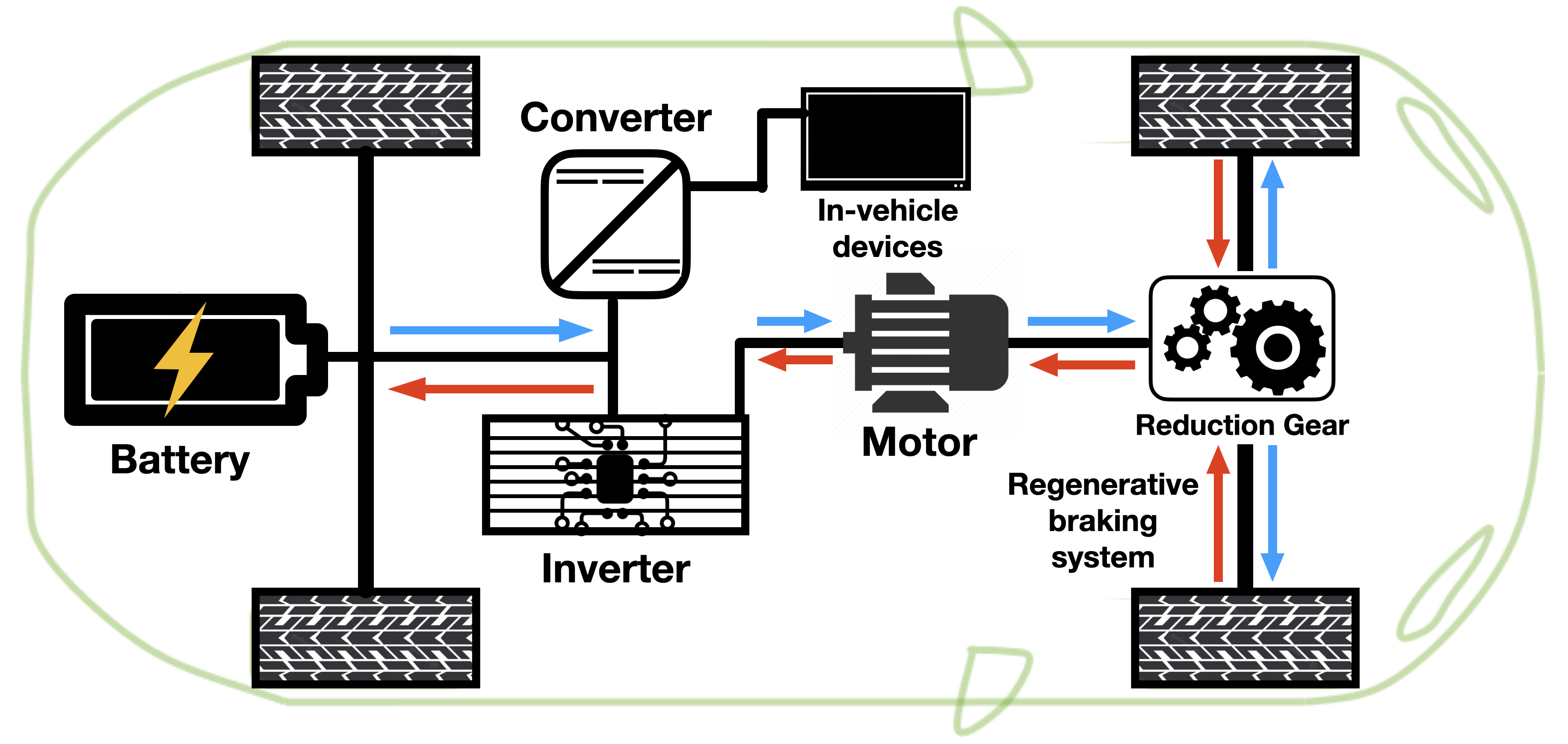
The EV powertrain consists of a battery, inverter, converter, reduction gear and one motor, and regenerative braking system, as shown in in Fig. 2. is the power that the motor receives from the battery or the power that the generator provides to the battery. Compared with the motor traction power, the loss in the power transmission, , and the power consumed by other in-vehicle auxiliary devices, , are relatively small, and the battery charging/discharging power is simplified as
| (4) |
From the rotational speed of the motor and wheel torque, the relation between the vehicle speed and force acting on the wheel can be obtained as
| (5) |
where and are the final gear-ratio and wheel radius, respectively.
For modeling and simulation, the electric motor data imported from ADVISOR [27] were analyzed to determine the motor’s regression model for energy consumption using the least squares method. The regression model was applied to the fifth-order polynomial in terms of and :
| (6) |
In the model fitting, the relative root mean square error (RRMSE) of the regressor (6) was 0.1917, for which the actual experimental data were used for training and validation.
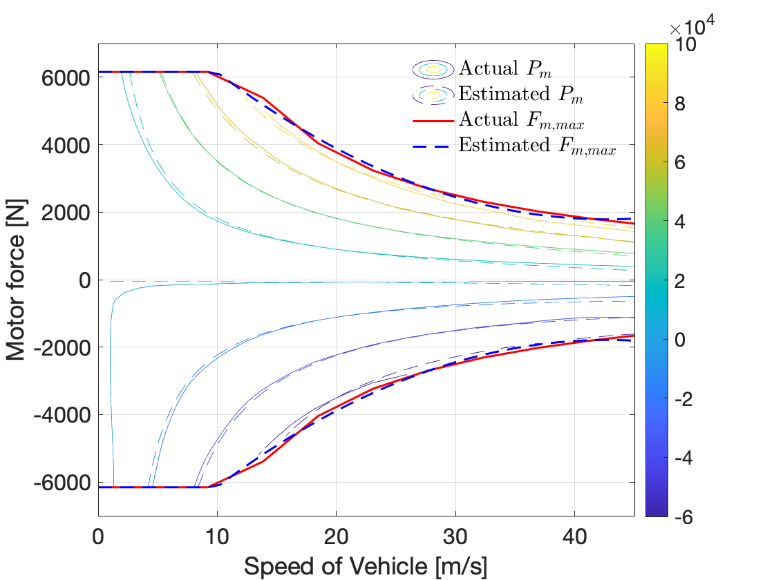
The maximum force that the motor can continuously generate is determined by the rotational speed of the motor, as shown in Fig. 3. Without tire slip, the speed of the vehicle and the force acting on the tire have a one-to-one correspondence and a constant value in the low vehicle-speed range, but tend to be inversely proportional to the speed of the vehicle in the high-speed range. The following regression models were used in this study:
| (7) |
where and denote the maximum and minimum motor forces in the low-speed range, respectively. In model fitting, the RRMSE of the regressor (7) was 0.3000, for which the actual experimental data were used for training and validation.
III Optimal Control Problem
For Eco-ACC, we considered the following constrained optimal control problem (OCP):
| (8) | ||||
where the host vehicle maintains a distance gap between m and m from the front vehicle and minimizes the energy in this process. This is considered as the objective function to be minimized in the optimal control problem.
IV Backgrounds in Solution Methods
IV-A Dynamic Programming
Dynamic programming was introduced by Bellman [28] as an algorithm that can find the global optimal solution of an optimal control problem. DP is based on the principle of optimality, that is, the optimization in future does not depend on the initial conditions and past-control inputs. The algorithm solves complex problems by dividing them into several small subproblems, and it reuses the solution of the subproblems in the process of solving complex problems.
IV-B Approximate Dynamic Programming
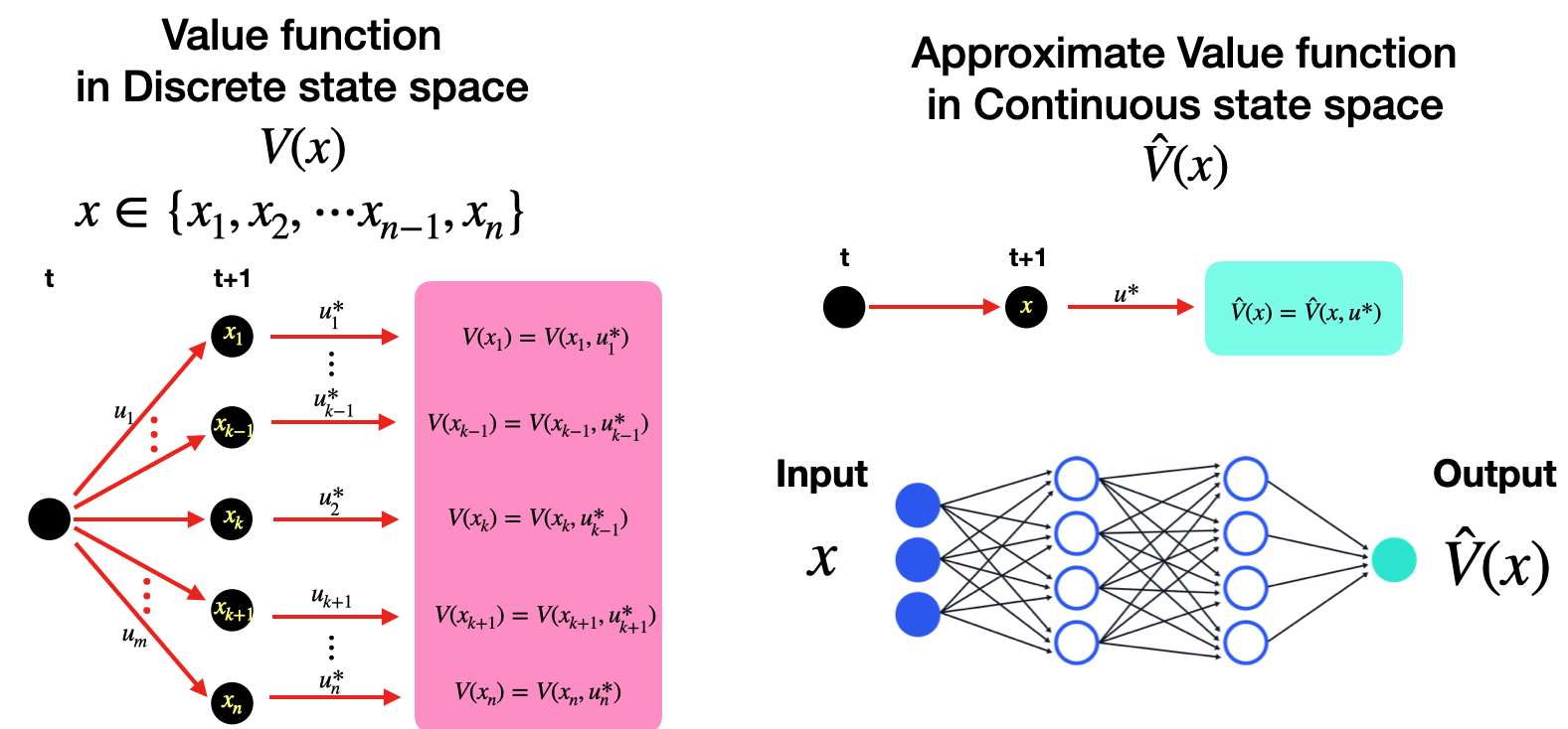
Approximate dynamic programming was introduced to resolve the problem of high computational resource requirements and the curse of dimensionality. Because the value function obtained in DP is calculated for discrete state space, it cannot be applied to a problem defined in a continuous state space. To solve this problem, ADP uses an approximate value function to use the value function calculated from the discrete state space in the continuous state space. Unlike DP, a suboptimal solution can be obtained using this method. The methods for obtaining the approximate value function are (i) polynomial regression, (ii) Gaussian process regression, and (iii) neural network approximation.
IV-C Reinforcement Learning
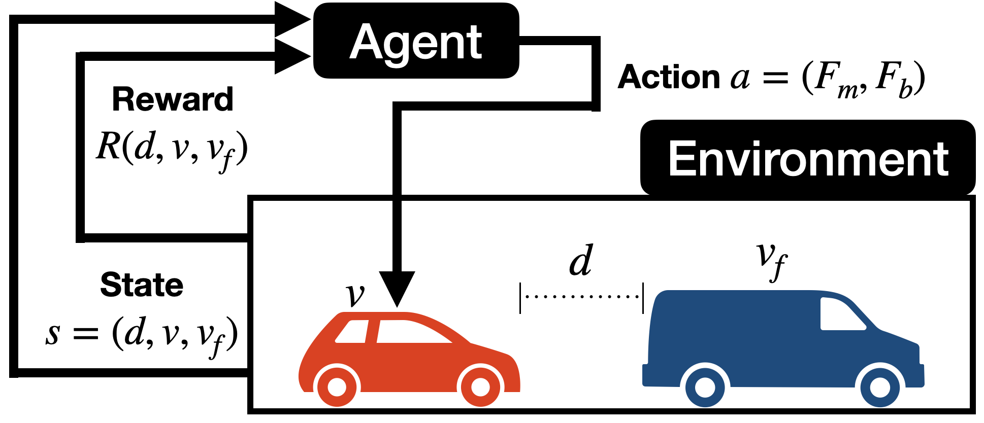
In this study, a typical framework of reinforcement learning [29] for Eco-ACC was configured, as shown in Fig. 4. The agent acts to maximize the cumulative rewards from the environment during the entire episode. At time , the agent receives an observation (or state) from the environment, performs action according to the current policy , and receives information about the state and reward from the environment; the same procedure is repeated until the end of the episode. Meanwhile, several reinforcement-learning techniques, such as value-based and policy-based RL, are the methods for the agent to learn.
For the RL agent, Deep Q-Network (DQN) [30] and Deep Deterministic Policy Gradient (DDPG) [31] were applied to solve the OCP 8 without using any models but only using data. Both RL methods are model-free and off-policy algorithms that use the Q-function approximation and the replay buffer. DQN is presented to solve the problem of unstable learning and divergence due to moving target value in Q-learning by introducing the replay buffer and the target network, but it can only handle discrete and low-dimensional action spaces. DDPG is an algorithm that combines the advantages of value-based and policy-based RL, which can overcome the limitations of the inability to directly apply Q-learning in continuous action spaces. The main idea of DDPG originates from the Deep Q-Network (DQN) algorithm [30]; however, DDPG uses two additional ideas. First, the algorithm uses the idea of actor–critic [32], that two different neural networks approximated by an actor network and a critic network, each of which has two networks, a main network and a target network, to train more softly. Second, instead of the -greedy method, DDPG adds noise to the deterministic action to promote exploration. The DDPG learning process is described in Algorithm 1.
Randomly initialize critic and actor
Initialize target networks :
,
Initialize replay buffer
V Solution Methods
To determine the energy-efficient acceleration/deceleration strategy, methods of DP, ADP, and RL were applied to find a solution for the optimal control problem described in Section III.
V-A Dynamic Programming
For the DP method, two methods are used to obtain the optimal solution:(i) DP-Backward and (ii) DP-Forward. In DP-Backward, a value table corresponds to the optimal cost-to-go from a set of quantized states. In DP-Forward, multistep look-ahead finite-horizon optimization is performed, in which a terminal-state penalty function approximates the optimal-cost-to-go.
In this study, the state variables and control inputs are quantized as follows:
| (9) |
where and are the state and control vectors, respectively.
V-A1 DP-Backward (Off-policy for computing the value table)
In the DP-Backward step, the input and state variables are quantized to calculate the value (i.e., optimal cost-to-go) table for
| (10) |
where the stage cost is and is the equi-spaced time interval of the sampling instances. In the DP-forward process, the speed profile of the host vehicle can be determined using the value table and the profile of the front vehicle. In this study, two speed profiles were generated under different conditions using the DP-based method:
-
•
DP-Forward I: One-step look ahead policy without considering any acceleration nor deceleration constraints;
-
•
DP-Forward II: Two-step look ahead policy with the value table computed offline.
They have different prediction horizons and control constraints, and their performances are compared in Section VI.
V-A2 DP-Forward I (One-step look ahead)
With the value table obtained from the DP-Backward process, the optimal control input and corresponding speed can be determined as
| (11) |
V-A3 DP-Forward II (Two-step look ahead)
The third DP-based methods of car-following speed planning is the two-step look ahead policy with the value table computed offline. By predicting the speed of the front vehicle for the next two steps using the previous two-step speed and via linear extrapolation, and can be determined as follows:
| (12) |
where is a concatenation of two successive control inputs. After the forward computation, the actual implementation follows a receding horizon scheme, similar to model predictive control. In principle, this forward process can be extended to multistep look ahead, but the computational burden increases with the prediction horizon. To remedy this curse of dimensionality, one can rely on the ADP methods that are briefly introduced in Section V-B.
V-B Approximate Dynamic Programming: Value Function Approximation
In the DP-based method, a value table was obtained for the set of quantized states in the DP-Backward process, and the energy-efficient optimal speed for the host vehicle was determined from the value table in the DP-Forward process. In the ADP-based method, the value table obtained in DP Backward V-A1 was approximated as a function using an artificial neural network, as shown in Fig. 5. Neural networks (NNs) are universal approximators which are extensively used in machine learning and artificial intelligence. For this study of OCP corresponding to Eco-ACC, NNs approximating the associated value function are used for modeling the MPC-like forward optimization of the continuous state and inputs. More specifically, we used an NN having three layers with 70 units in each layer, and a sigmoid function was used as the activation function in the hidden layers. The error in the approximate value-function data from the DP-based value table was 0.0955 in the RRMSE.
V-C Reinforcement Learning
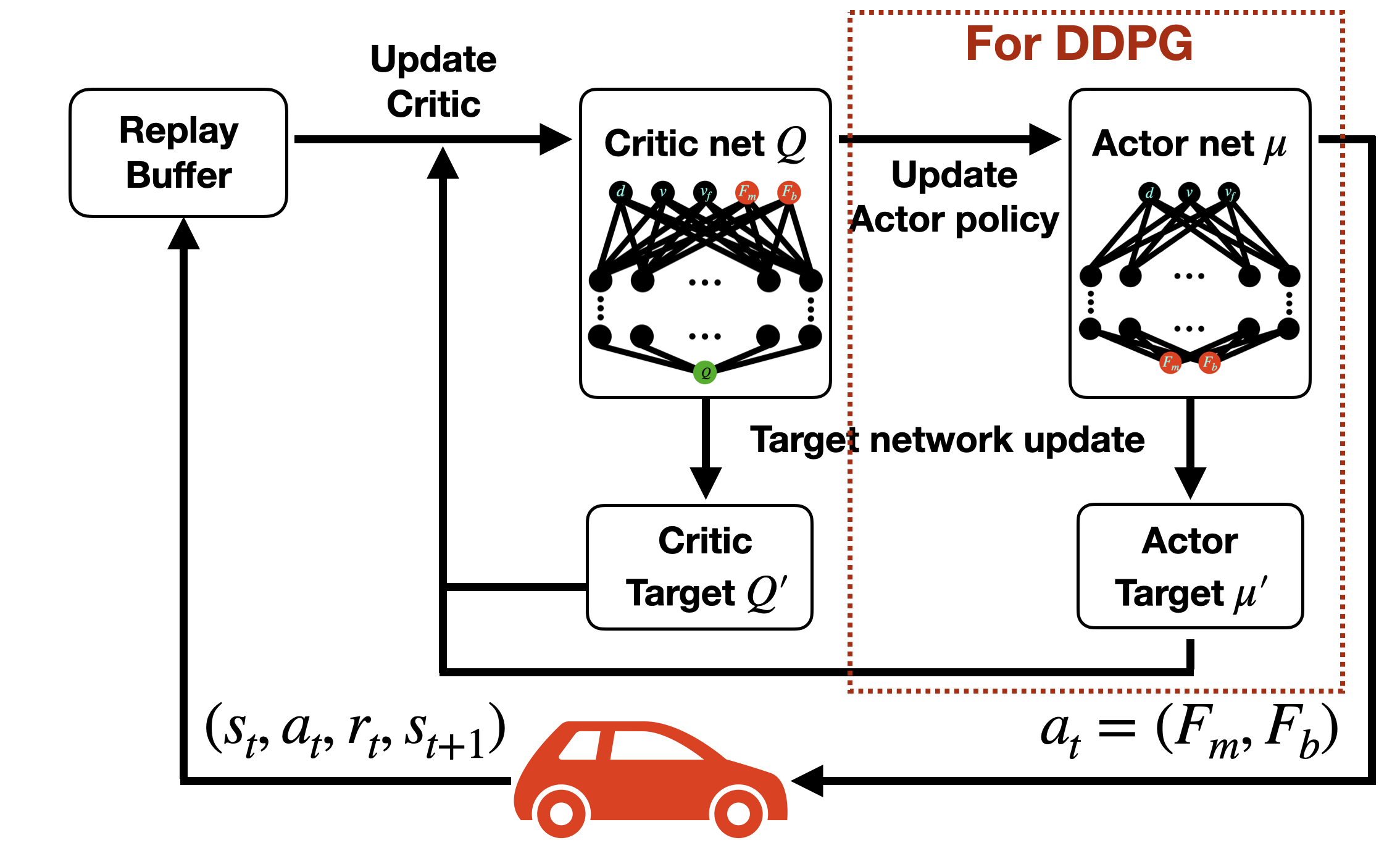
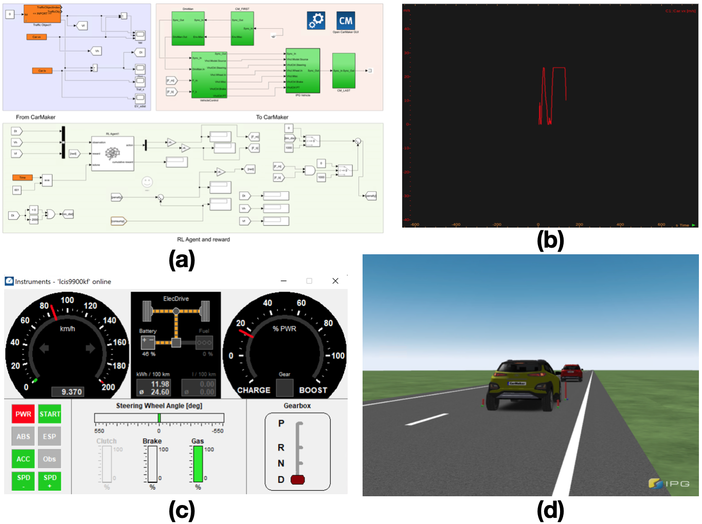
To allow the RL agents to learn the energy-efficient Eco-ACC policy from trial and error, the training environment shown in Fig. 6 was established based on MATLAB/Simulink and IPG CarMaker, as shown in Fig. 7. During an episode, the simulation environment provides observations and reward based on the action. The transition is stored in the replay buffer and is used to update the main critic and main actor accordingly. And updates the target networks : and . At the next moment, the process of performing an action according to the deterministic policy and exploration noise is repeated. For DQN, the critic networks and are updated only and the control action is selected according to the -greedy method.
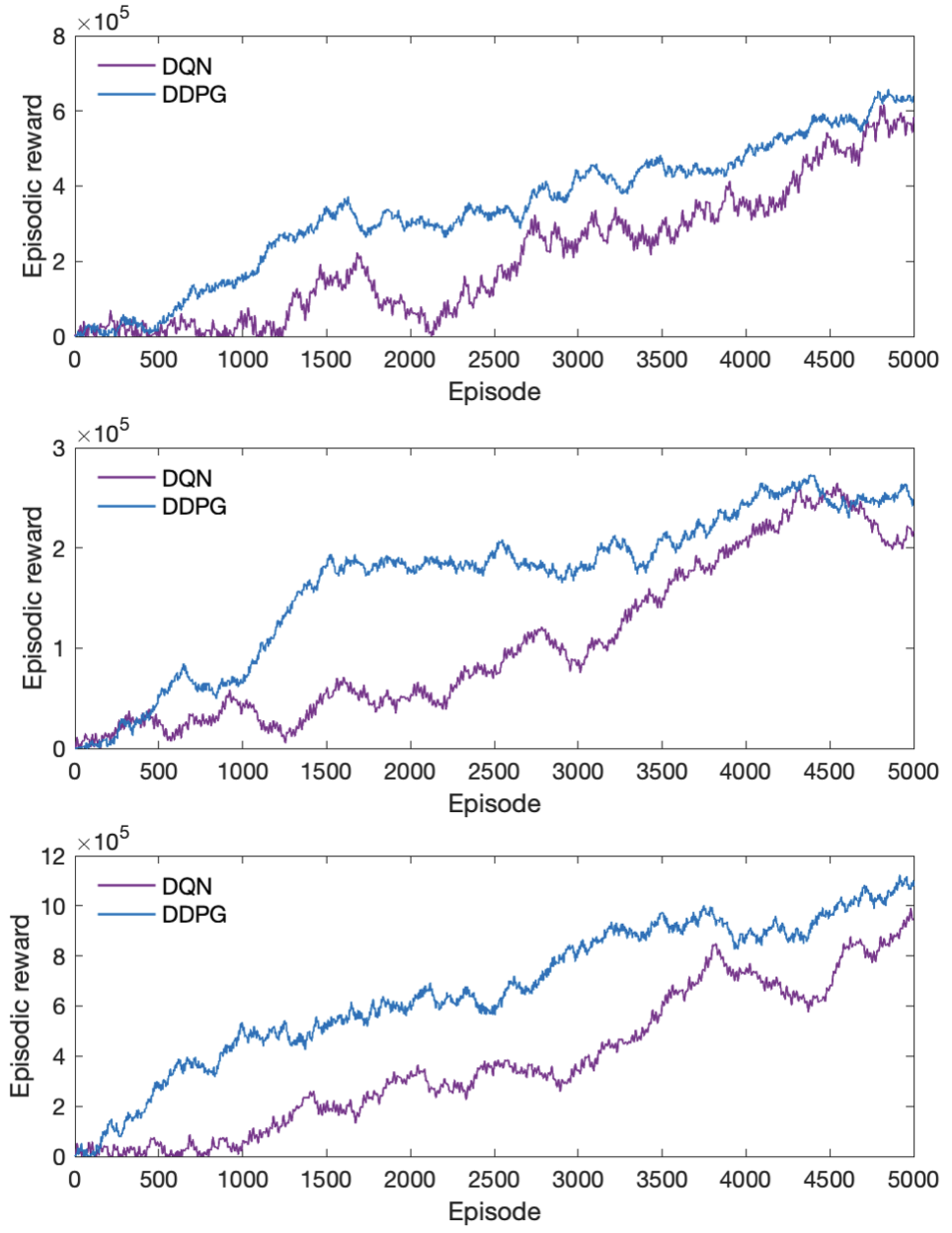
In the training process, the reward received by the agent from the environment is shown in table I. In order to minimize the energy consumption while driving on one episode, the negative value of motor power . In addition, always ensure that agents are rewarded by 1000, except when the distance to the vehicle ahead becomes 0 m (collision) or exceeds 2000 m (too much gap from the front vehicle). Finally, the agent is also rewarded, provided . In this study, 5,000 training sessions were conducted for each scenario to train the RL agents. Fig. 8 shows the episodic rewards computed during the training process.
| Objective or Condition | Value | |
| Minimizing energy consumption | ||
| Maintaining distance gap range | True | 1000 |
| False | 0 | |
| Acceleration/Deceleration only | True | 1000 |
| False | 0 | |
| Hyperparameters | |||
| Description | Value | Description | Value |
| Actor network layers | 2 | Critic network layers | 3 |
| Number of units per critic network layer | 256 | Number of units per critic network layer | 70 |
| Actor learning rate | 0.01 | Critic learning rate | 0.01 |
| Discount factor | 0.99 | Replay buffer size | 5000 |
| Target smooth factor | 0.005 | Batch size | 64 |
| Symbol | Description | Value |
| Vehicle mass | 1600 [kg] | |
| Coefficient of drag | 0.373 [-] | |
| Frontal projected area of vehicle | 2.0107 [] | |
| Air density | 1.2 [] | |
| Coefficient of rolling resistance | 0.0088 [-] | |
| Gravitational constant | 9.81 [] | |
| Gear ratio of final reduction drive | 7.4 [-] | |
| Wheel radius | 0.326 [m] | |
| Road slope |
VI Simulation Results
To verify the strategy obtained from the method presented in Section V, we considered three different scenarios according to the speed profile of the front vehicle. The front vehicle are assumed to drive according to the speed profiles of either
-
•
Scenario 1: the HWFET cycle, representing highway driving conditions under 60 [mph],
-
•
Scenario 2: the US06 cycle, representing high acceleration aggressive driving, or
-
•
Scenario 3: the WLTP Class 3b cycle, representing European and Japanese commercial vehicles with a maximum speed of above 120 [kph].
The host vehicle follows the front vehicle while minimizing energy consumption. For DP and ADP, simulations were performed in IPG CarMaker [33] based on the speed profile of the host vehicle obtained from DP and ADP-Forward. For the RL method, a Simulink environment with a DDPG agent and reward function was constructed with the CarMaker extension. A video recording of the simulation is available at https://youtu.be/DIXzJxMVig8.
VI-A Dynamic Programming-Based method
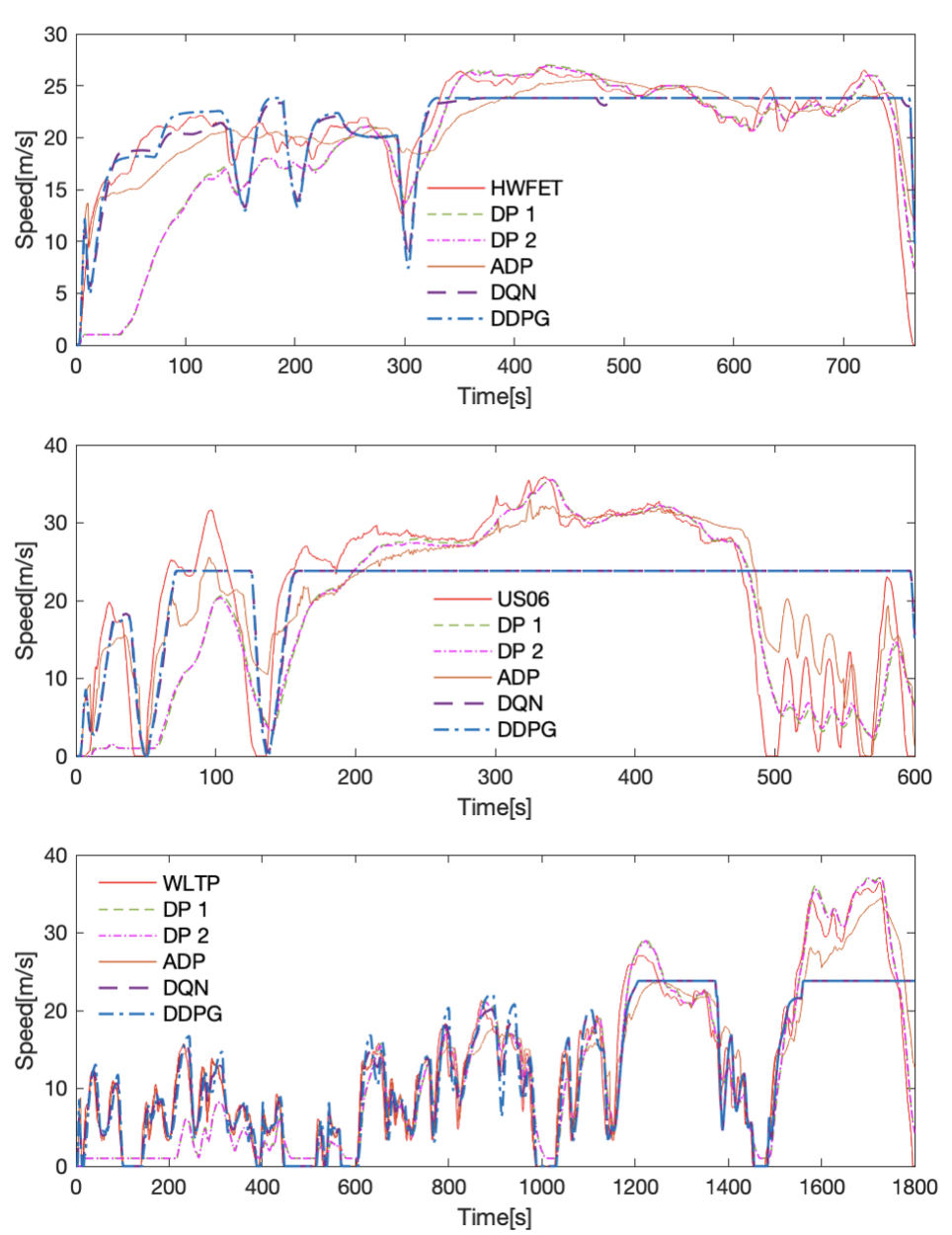
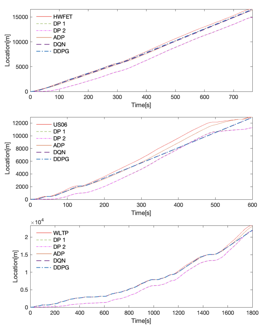
For the presented optimal control problem, a value table for each state was obtained from DP-Backward. Based on the value table, an optimal speed profile was obtained for the host vehicle. The simulation was conducted as follows. The virtual host vehicle was driven in CarMaker according to the generated speed profiles. The energy efficiency was measured using CarMaker.
It can be observed that the frequency of rapid acceleration and deceleration is lower than that of the front vehicle. In addition, a relatively gradual speed profile can be observed while maintaining the range of the distance gap. In other words, it can be observed that relatively gradual acceleration and deceleration strategies appear as a result of relatively high energy efficiency.
The same simulation procedure was performed for the front vehicle moving according to the US06 Profile. Similar to Scenario 1, the speed profile obtained from the DP demonstrated better energy efficiency than that of the front vehicle with more moderate sensitivity/acceleration. Notably, it can be observed that the DP2 speed profile with 2-step lookahead indicates a relatively poor energy efficiency compared to DP1 with 1-step lookahead. This is because the distance gap with the front vehicle is initially widened, and then the speed of the front vehicle between 500 and 600 [s] is predicted at 2-step lookahead, which is a relatively rapid acceleration/deceleration compared to that of DP1 to ensure the maintenance of the range of the distance gap.
For the scenario with the front vehicle following the WLTP Class 3b driving cycle, both DP vehicles exhibited approximately 6% higher energy efficiency than the front vehicle. It should be noted that, similar to Scenario 1, DP1 and DP2 showed almost the same energy efficiency. Because there is a relatively less rapid acceleration/deceleration of the front vehicle, the prediction of 2-step lookahead DP can affect the overall energy efficiency improvement, and the energy efficiency of the DP1 and DP2 results did not show much difference.
VI-B Approximate Dynamic Programming-Based Method
Similar to the previous DP-based method, the speed profile is obtained by applying 2-step lookahead and the energy efficiency is measured by IPG CarMaker. The simulation results for Scenario 1 showed that the energy efficiency of ADP was 3.5% higher than that of the front vehicle and 0.4% higher than that of DP2. In the case of DP2, acceleration begins when the distance gap approaches the constraint limit of 2000 [m], whereas ADP starts acceleration when the distance gap is less than DP2. It can also be observed that the energy efficiency is similar even though it travels more distance than DP2. Similar to DP2, ADP exhibited better energy efficiency than the front vehicle. However, because acceleration begins relatively earlier than DP2, rapid acceleration and deceleration between 0 and 50 [s] is presumed to be the cause of the energy efficiency was lower by 6.3% compared to DP2. For Scenario 3, ADP showed more travel distance and higher energy efficiency compared with the front vehicle and DP2.
VI-C Reinforcement Learning-Based method
The traveling speed and distance profiles shown in Figs. 9 and 10, respectively, were obtained using the 5,000-times trained DQN and DDPG agents. Unlike the DP and ADP results, the RL-host vehicle tends to drive while maintaining the maximum energy-efficient speed (approximately [m/s]). In particular, the US06 scenario achieved the result of driving at a constant speed despite the large distance from the vehicle ahead. However, the RL-Host vehicle does not drive fast in the WLTP scenario. The vehicle accelerates and decelerates in the low-speed range, and, in the latter part of the scenario, it tends to drive at a speed of approximately [m/s], except for the low-speed range of 14001600 [s]. As results, energy efficiency was improved by about 13.9% (for DQN) and 14.8% (for DDPG) on average of three scenarios when compared to the front vehicle.
| Scenario 1 : HWFET front vehicle | |||
| Car | Travel Distance [m] | Efficiency [km/kWh] | Ratio [%] |
| HWFET | 16556.08 | 8.5543 | 100.0 |
| DP 1 | 14955.48 | 8.7719 | 102.5 |
| DP 2 | 14922.23 | 8.7873 | 102.7 |
| ADP | 16314.00 | 8.8183 | 103.1 |
| DQN | 16314.00 | 8.8183 | 104.3 |
| DDPG | 16222.86 | 8.9686 | 104.8 |
| Scenario 2 : US06 front vehicle | |||
| Car | Travel Distance [m] | Efficiency [km/kWh] | Ratio [%] |
| US06 | 12938.56 | 5.6370 | 100.0 |
| DP 1 | 11280.08 | 6.7159 | 119.1 |
| DP 2 | 11283.19 | 6.7431 | 119.6 |
| ADP | 12934.91 | 6.3857 | 113.3 |
| DQN | 12689.71 | 6.7431 | 124.3 |
| DDPG | 12704.54 | 7.0274 | 124.7 |
| Scenario 3 : WLTP class 3b front vehicle | |||
| Car | Travel Distance [m] | Efficiency [km/kWh] | Ratio [%] |
| WLTP | 23312.39 | 7.5131 | 100.0 |
| DP 1 | 21807.45 | 7.9681 | 106.1 |
| DP 2 | 21763.19 | 7.9681 | 106.1 |
| ADP | 23008.76 | 8.3195 | 110.7 |
| DQN | 21988.91 | 8.5071 | 113.2 |
| DDPG | 22026.62 | 8.5616 | 113.9 |
VII Conclusions and Future Work
This paper proposed and compared learning-based methods (ADP, DQN and DDPG) for energy-efficient Eco-ACC for connected EVs. An optimal control problem with constraints was formulated based on the EV model to minimize the energy consumption while satisfying the physical limits of actuation commands and avoiding a collision. For model-based learning, ADP, a neural network, was used for value function approximation, and multi-step look-ahead receding horizon control was applied in the forward direction. For model-free learning, we applied DQN and DDPG in which neural networks were used to train the state-action value function and deterministic policy. High-fidelity simulations using IPG CarMaker demonstrated the performance and effectiveness of the proposed learning methods for Eco-ACC. Our future work will involve performing hardware-in-the-loop-simulation (HiLS) using dSPACE MicroAutoBox II to further validate the feasibility of a real-time energy-efficient acceleration and deceleration strategy.
References
- [1] Z. Li, A. Khajepour, and J. Song, “A comprehensive review of the key technologies for pure electric vehicles,” Energy, vol. 182, pp. 824–839, 2019.
- [2] C. C. Chan, “The state of the art of electric, hybrid, and fuel cell vehicles,” Proceedings of the IEEE, vol. 95, no. 4, pp. 704–718, 2007.
- [3] D. Watzenig and B. Brandstätter, Comprehensive Energy Management: Eco Routing & Velocity Profiles. Springer, 2017, vol. 770.
- [4] L. Guzzella and A. Sciarretta, Vehicle Propulsion Systems: Introduction to Modeling and Optimization. Springer Berlin, Heidelberg, 2013.
- [5] A. Vahidi and A. Sciarretta, “Energy saving potentials of connected and automated vehicles,” Transportation Research Part C: Emerging Technologies, vol. 95, pp. 822–843, 2018.
- [6] A. G. Boulanger, A. C. Chu, S. Maxx, and D. L. Waltz, “Vehicle electrification: Status and issues,” Proceedings of the IEEE, vol. 99, no. 6, pp. 1116–1138, 2011.
- [7] M. Ehsani, Y. Gao, S. Longo, and K. Ebrahimii, Modern Electric, Hybrid Electric, and Fuel Cell Vehicles. CRC Press, 2018.
- [8] A. Sciarretta, G. De Nunzio, and L. L. Ojeda, “Optimal ecodriving control: Energy-efficient driving of road vehicles as an optimal control problem,” IEEE Control Systems, vol. 35, no. 5, pp. 71–90, 2015.
- [9] J. Guanetti, Y. Kim, and F. Borrelli, “Control of connected and automated vehicles: State of the art and future challenges,” Annual Reviews in Control, vol. 45, pp. 18–40, 2018.
- [10] E. Ozatay, S. Onori, J. Wollaeger, Ü. Özgüner, G. Rizzoni, D. Filev, J. Michelini, and S. D. Cairano, “Cloud-based velocity profile optimization for everyday driving: A dynamic-programming-based solution,” IEEE Transactions on Intelligent Transportation Systems, vol. 15, pp. 2491–2505, 2014.
- [11] D. Kim, J. S. Eo, and K.-K. K. Kim, “Parameterized energy-optimal regenerative braking strategy for connected and autonomous electrified vehicles: A real-time dynamic programming approach,” IEEE Access, vol. 9, pp. 103 167–103 183, 2021.
- [12] ——, “Service-oriented real-time energy-optimal regenerative braking strategy for connected and autonomous electrified vehicles,” IEEE Transactions on Intelligent Transportation Systems, vol. 23, no. 8, pp. 11 098–11 115, 2022.
- [13] D. Shen, D. Karbowski, and A. Rousseau, “A minimum principle-based algorithm for energy-efficient eco-driving of electric vehicles in various traffic and road conditions,” IEEE Transactions on Intelligent Vehicles, vol. 5, no. 4, pp. 725–737, 2020.
- [14] H. Lim, C. C. Mi, and W. Su, “A distance-based two-stage ecological driving system using an estimation of distribution algorithm and model predictive control,” IEEE Transactions on Vehicular Technology, vol. 66, no. 8, pp. 6663–6675, 2017.
- [15] H. Lee, N. Kim, and S. W. Cha, “Model-based reinforcement learning for eco-driving control of electric vehicles,” IEEE Access, vol. 8, pp. 202 886–202 896, 2020.
- [16] S. Bae, Y. Kim, J. Guanetti, F. Borrelli, and S. Moura, “Design and implementation of ecological adaptive cruise control for autonomous driving with communication to traffic lights,” in American Control Conference (ACC), 2019, pp. 4628–4634.
- [17] Y. Jia, R. Jibrin, and D. Görges, “Energy-optimal adaptive cruise control for electric vehicles based on linear and nonlinear model predictive control,” IEEE Transactions on Vehicular Technology, vol. 69, no. 12, pp. 14 173–14 187, 2020.
- [18] D. P. Bertsekas, Dynamic Programming and Optimal Control. Belmont, MA, USA: Athena Scientific, 2005.
- [19] R. Bellman, “The theory of dynamic programming,” Bulletin of the American Mathematical Society, vol. 60, no. 6, pp. 503–515, 1954.
- [20] W. B. Powell, Approximate Dynamic Programming: Solving the Curses of Dimensionality. Hoboken, NJ, USA: Wiley, 2007.
- [21] L. Johannesson and B. Egardt, “Approximate dynamic programming applied to parallel hybrid powertrains,” International Federation of Automatic Control Proceedings Volumes, vol. 41, no. 2, pp. 3374–3379, 2008.
- [22] M. P. Deisenroth, J. Peters, and C. E. Rasmussen, “Approximate dynamic programming with gaussian processes,” in American Control Conference (ACC), 2008, pp. 4480–4485.
- [23] M. P. Deisenroth, C. E. Rasmussen, and J. Peters, “Gaussian process dynamic programming,” Neurocomputing, vol. 72, no. 7–9, pp. 1508–1524, 2009.
- [24] J. W. Bae and K.-K. K. Kim, “Gaussian process approximate dynamic programming for energy-optimal supervisory control of parallel hybrid electric vehicles,” IEEE Transactions on Vehicular Technology, 2022, (Early Access). [Online]. Available: DOI:10.1109/TVT.2022.3178146
- [25] M. Zhou, Y. Yu, and X. Qu, “Development of an efficient driving strategy for connected and automated vehicles at signalized intersections: A reinforcement learning approach,” IEEE Transactions on Intelligent Transportation Systems, vol. 21, no. 1, pp. 433–443, 2020.
- [26] M. Wegener, L. Koch, M. Eisenbarth, and J. Andert, “Automated eco-driving in urban scenarios using deep reinforcement learning,” Transportation Research Part C: Emerging Technologies, vol. 126, p. 102967, 2021.
- [27] T. Markel, A. Brooker, T. Hendricks, V. Johnson, K. Kelly, B. Kramer, M. O’Keefe, S. Sprik, and K. Wipke, “ADVISOR: A systems analysis tool for advanced vehicle modeling,” Journal of Power Sources, vol. 110, no. 2, pp. 255–266, 2002.
- [28] R. Bellman, Dynamic Programming. Princeton University Press, Princeton, NJ, USA, 1957.
- [29] R. S. Sutton and A. G. Barto, Reinforcement Learning: An Introduction, 2nd ed. Cambridge, MA, USA: The MIT Press, 2018.
- [30] V. Mnih, K. Kavukcuoglu, D. Silver, A. Graves, I. Antonoglou, D. Wierstra, and M. Riedmiller, “Playing atari with deep reinforcement learning,” arXiv preprint arXiv:1312.5602, 2013.
- [31] T. P. Lillicrap, J. J. Hunt, A. Pritzel, N. M. O. Heess, T. Erez, Y. Tassa, D. Silver, and D. Wierstra, “Continuous control with deep reinforcement learning,” International Conference on Learning Representations, vol. abs/1509.02971, 2016.
- [32] V. Konda and J. Tsitsiklis, “Actor-critic algorithms,” in SIAM Journal on Control and Optimization. MIT Press, 2000, pp. 1008–1014.
- [33] IPG Automotive GmbH, “IPG CarMaker.” [Online]. Available: https://ipg-automotive.com/en/