Learning county from pixels: Corn yield prediction with attention-weighted multiple instance learning

Abstract

Remote sensing technology has become a promising tool in yield prediction. Most prior work employs satellite imagery for county-level corn yield prediction by spatially aggregating all pixels within a county into a single value, potentially overlooking the detailed information and valuable insights offered by more granular data. To this end, this research examines each county at the pixel level and applies multiple instance learning to leverage detailed information within a county. In addition, our method addresses the “mixed pixel” issue caused by the inconsistent resolution between feature datasets and crop mask, which may introduce noise into the model and therefore hinder accurate yield prediction. Specifically, the attention mechanism is employed to automatically assign weights to different pixels, which can mitigate the influence of mixed pixels. The experimental results show that the developed model outperforms four other machine learning models over the past five years in the U.S. corn belt and demonstrates its best performance in 2022, achieving a coefficient of determination ($R^{2}$) value of 0.84 and a root mean square error (RMSE) of 0.83. This paper demonstrates the advantages of our approach from both spatial and temporal perspectives. Furthermore, through an in-depth study of the relationship between mixed pixels and attention, it is verified that our approach can capture critical feature information while filtering out noise from mixed pixels.

[inst1]organization=Biological Systems Engineering,addressline=University of Wisconsin-Madison, city=Madison, postcode=53706, state=WI, country=USA

[inst2]organization=Department of Earth System Science and Center on Food Security and the Environment,addressline=Stanford University, city=Stanford, postcode=94305, state=CA, country=USA

[inst3]organization=Department of Geography,addressline=University of Wisconsin-Madison, city=Madison, postcode=53706, state=WI, country=USA

[inst4]organization=Research and Development Division, National Agricultural Statistics Service,addressline=United States Department of Agriculture, city=Washington, postcode=20250, state=DC, country=USA

1 Introduction

County-level corn yield prediction in the U.S. holds significant importance due to its central role in the country’s agriculture and economy (Shuai and Basso, 2022; Yang et al., 2021; Ma et al., 2021a). Accurate predictions enable better planning for supply chain management, price setting, and policy-making, as well as assisting farmers in the decision-making process to optimize resource use. Due to the advantages of efficiency, cost-effectiveness, easy data acquisition, wide spatial coverage, and short operating cycles, remote sensing (RS) technology has been widely applied in yield prediction (Deines et al., 2021; Jin et al., 2019; Battude et al., 2016). RS for yield prediction typically involves two main approaches: process-based method (Bastiaanssen and Ali, 2003; Huang et al., 2015; Mishra et al., 2013; Lobell and Burke, 2010) and learning-based method (Shuai and Basso, 2022; Ma et al., 2021a). The former utilizes mathematical models to represent and simulate the physical and biological processes that determine crop growth and development. The latter predicts yield by learning the complex and non-linear relationships between yield and features extracted from RS data. As a data-driven approach, the learning-based method is capable of quickly processing large volumes of data generated by RS technologies, leading to enhanced generalization for more accurate yield predictions on new data, without the need for explicitly modeling the physical processes as in the process-based method (Sakamoto et al., 2014; Johnson, 2014a; Sakamoto et al., 2013). Therefore, this study focuses on exploring using a learning-based method for county-level corn yield prediction.

Among all learning-based models, deep learning (Goodfellow et al., 2016) is currently the most popular and effective. Many studies have investigated the use of various types of neural networks with RS data for the yield prediction task. One of the earliest forms of neural network, Multi-Layer Perceptron (MLP) (Haykin, 1998) consists of multiple layers of nodes in a directed graph for understanding complex data. Khaki and Wang (2019) employs MLPs to forecast yields using data on genotype and environmental factors, comprehending nonlinear and intricate correlations among genetic factors, environmental variables, and their interplay. Additionally, Convolutional Neural Network (CNN) (LeCun et al., 1995) uses a mathematical operation called convolution, which is highly effective in processing images. Nevavuori et al. (2019) establishes a combined model for wheat and barley yield prediction in the Finnish continental subarctic climate, indicating that the CNN models are capable of reasonably accurate yield estimates based on RGB images. For time series modeling, Recurrent Neural Network (RNN) (Rumelhart et al., 1985) has internal memory that captures information about previous steps. Khaki et al. (2020) introduces a hybrid model that integrates both CNNs and RNNs, where the RNN component is focused on tracking the upward trajectory in crop yields over time due to continuous improvement in plant breeding and management practices. Recently, Transformer (Vaswani et al., 2017) has significantly improved the performance in various language tasks relying on self-attention mechanism and has been the foundation for large language models. Liu et al. (2022) proposes a transformer-backbone model to predict district-level rice yield based on multi-temporal satellite data, sequential climatic products, and historical rice yield, which shows significant capability in integrating various types of data. These studies demonstrate the vast potential and rapid development of deep learning in the fields of RS and yield prediction.

In county-level yield prediction, many previous studies treat a county as a unified entity, aggregating all pixels within the county to a single value (e.g. mean value) (Shahhosseini et al., 2021; Wang et al., 2020; Sakamoto et al., 2014; Ma et al., 2021a). This method simplifies the model by transforming all corn pixel values within a county into a single statistical value, considerably reducing the computational load. Moreover, averaging the variations within the county may result in more consistent and resilient predictions. For example,  Wang et al. (2020) develops a dual-branch deep learning framework for county-level winter wheat yield prediction, where all RS information is spatially consolidated to the average value of each county.  Ma et al. (2021a) employs a Bayesian neural network for county-level corn yield prediction to offer both prompt yield estimation and its corresponding predictive uncertainty. This approach extracts time-series vegetation indices (VIs), climate observations, and soil properties from multiple data sources and aggregates them to the county level. Furthermore, utilizing the median instead of a straightforward average effectively reduces the influence of outliers on the yields.  Shahhosseini et al. (2021) examines the possibility of enhancing the performance of machine learning models by incorporating variables from simulated crop models as input. This method computes the features for each county and employs the median of all associated values as input. However, aggregating all the pixels within the county to a single value may compromise the integrity of county data representation, potentially losing detailed information. As a result, missing crucial information could substantially reduce the model’s predictive performance. Therefore, all corn pixel data from each county are collected and utilized as completely as possible to predict the county’s yield, thereby enhancing the accuracy and reliability of the prediction.

Multiple instance learning (MIL) (Dietterich et al., 1997; Carbonneau et al., 2018) is a variant of a supervised machine learning method. In traditional supervised learning, an instance refers to a single data point or observation, each instance has one corresponding label, whereas in MIL, labels are associated with “bags” rather than the individual “instances” contained within them. It leverages the detailed information contained within a bag to predict the label of the entire bag, even though individual instances inside the bag are not explicitly labeled. When predicting county-level corn yield by treating a county as an aggregation of all individual pixels, each county can be designated as a bag and its comprising distinct pixels can be treated as instances to fit county-level corn yield into the MIL framework. There are a few factors that prompt us to investigate using MIL for county level corn yield prediction modeling. First, the MIL allows for nuanced use of detailed information within a county for predicting yield, and can potentially discern underlying patterns within a county to aid the learning progress. Second, given that satellite imagery has a large number of bands and extremely large data volume, fully utilizing all images for modeling requires large amounts of computational resources. In addition, different counties contain varying numbers of pixels, which also presents a challenge for batch processing. To address the computational resources issue, MIL often adopts a sampling method to select the most important instances in a bag (Sec. 3.5), thus better striking a balance between data volume and model accuracy. Third, in our scenario, only pixel-level RS imagery is available, but pixel-level yield records are lacking, making end-to-end pixel-level learning and analysis difficult. However, MIL can train models and make predictions even without instance labels, addressing the end-to-end pixel-level learning challenge.

When analyzing satellite imagery or its derivative datasets at the pixel level, it often comes across a challenge commonly referred to as the “mixed pixel” problem (Xu et al., 2005) due to the inconsistent resolution between crop mask and various feature datasets. Learning-based corn yield prediction often utilizes corn field feature data collected from satellite data and its derivative data products to build a model. To predict corn yield, it is common to use a crop mask to identify the corn fields within the study area. We will use MODIS dataset (Justice et al., 1998; Schaaf and Wang, 2015) as a primary example to illustrate this problem. For example, LABEL:fig:mixedmodis (a) shows a patch of land containing corn, bare soil and weeds, with the shaded region in the middle representing a MODIS pixel. The resolution of MODIS data is $500\mathrm{m}\times 500\mathrm{m}$. LABEL:fig:mixedmodis (b) displays the MODIS pixel masked by CDL (USDA-NASS, 2017), where the green portion signifies land planted with corn, the blue portion indicates unrelated land types, and the resolution of the CDL mask is $30\mathrm{m}\times 30\mathrm{m}$. When using CDL to extract corn-specific land, the VIs of a single CDL pixel are calculated from the encompassing larger MODIS pixel that contains this smaller CDL pixel. This MODIS pixel may cover both corn fields and other land types, mixing the VIs’ information from these different land categories. We call the $30\mathrm{m}\times 30\mathrm{m}$ CDL pixel a “mixed pixel”. It is essential to highlight that actually the big MODIS pixel is a mixed pixel, however in this paper, our focus is the finer-resolution CDL pixels which share information of the mixed VIs. In subsequent sections, any reference to a mixed pixel is explicitly related to the smaller CDL pixel. Furthermore, it is worth noting that merely increasing the resolution of the crop mask does not solve the mixed pixel issue, given that the satellite imagery’s resolution is inherently limited. Additionally, while we use the satellite imagery MODIS dataset as an illustration, our experiment includes other features such as weather, soil properties, etc. In fact any features whose resolution is lower than CDL mask can also present the mixed pixel problem. In Fig. 2, one pixel of PRISM dataset (Daly et al., 2015) with $4\mathrm{km}\times 4\mathrm{km}$ resolution is masked by CDL, and all the $30\mathrm{m}\times 30\mathrm{m}$ CDL pixels in this PRISM pixel share the same PRISM features value. To effectively address the mixed pixel issue, we propose to use an attention mechanism (Vaswani et al., 2017) to make rational use of the information of those mixed pixels.

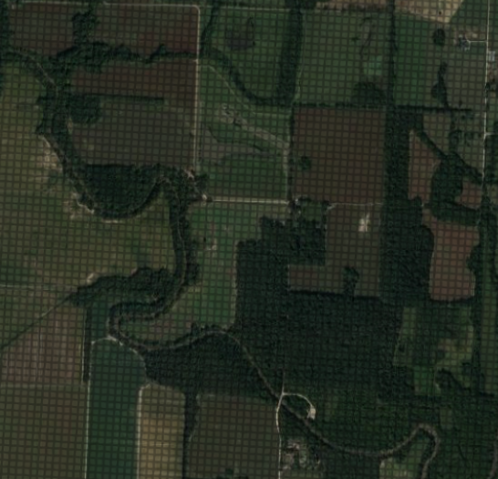
Figure 2: This figure demonstrates one cell on the RS imagery in PRISM dataset masked by many small CDL cells.

The attention mechanism (Vaswani et al., 2017; Ilse et al., 2018) is a powerful tool in deep learning. It enables models to address specific aspects of complex input data. Essentially, it can be used to assign different weights or “attention scores” to different parts of the input. This weighting mechanism is analogous to the way human beings pay attention to certain details while ignoring others (Khan et al., 2022). To address the mixed pixel problem, we will use this mechanism to allocate higher weights to pixels predominantly comprising cropland and lower weights to those with more irrelevant categories, thereby boosting the model’s accuracy and interpretability. This method effectively utilizes the information of each pixel while avoiding the detrimental impact of the mixed pixels, and thereby enhances the accuracy of our prediction. Furthermore, the results from applying attention weights to pixels reveal a tight correlation among attention scores, agricultural features, and the cropland ratio in mixed pixels ( Sec. 5).

Many previous studies apply the combination of the attention mechanism and MIL. For example, Ilse et al. (2018) introduces a versatile and understandable MIL method completely driven by neural networks, along with a trainable MIL pooling using the gated attention mechanism. (Rymarczyk et al., 2021) incorporates self-attention into the process of MIL Pooling, merging the multi-level dependencies among different image areas with a trainable weighted average pooling mechanism. (Hu et al., 2023) introduces a new MIL technique for medical image analysis named triple-kernel gated attention-based MIL with contrastive learning instead of using ImageNet for pre-training. While the above studies explore the combination of attention and MIL, the purpose of this work is not to enhance the performance of downstream tasks with MIL and attention mechanism. The aim is instead to effectively harness detailed information with MIL, followed by resolving the mixed pixel problem with attention. These are two progressive yet parallel objectives.

In summary, this paper presents a new method to improve county-level corn yield prediction. It leverages the MIL framework to utilize detailed information from individual pixels within each county, thereby enhancing performance. To tackle the mixed pixel problem, our method uses the attention mechanism to automatically learn a weight for each pixel, representing the contribution of each pixel to the final prediction results. To our knowledge, we are the first to use attention to solve the mixed pixel problem in county-level corn yield prediction.

This paper is organized as follows. Sec. 1 introduces background about corn crop yield models, the challenge faced, and the objective of this paper. Sec. 2 describes the study area, experimental model input data, experiment design, and experiment result evaluation. Sec. 3 describes the model overview of proposed attention-weighted MIL method including problem definition, attention mechanism, and sampling method. Sec. 4 discusses experiment results, abnormal results, and shows some detailed analysis from both spatial and temporal perspectives. Sec. 5 delves into attention analysis and correlation of attention with features. Finally, Sec. 6 presents conclusions of this research.

2 Data acquisition

2.1 Study area

The study area covers twelve corn belt states in the United States, including North Dakota, South Dakota, Minnesota, Wisconsin, Iowa, Illinois, Indiana, Ohio, Missouri, Kansas, Nebraska and Michigan (Fig. 3), wherein we calculate the average corn yield for all states from 2008 to 2022. Darker colors represent higher yields. For other regions, we note that although the states surrounding Idaho in the top-left corner display a dark color, their area dedicated to corn cultivation is relatively limited. Additionally, the broader region in the southeast has a more significant corn-growing area, yet the yield there is comparatively lower. So it is evident that we only need data from these twelve states for our study. The corn production in the selected states accounts for most of the major US corn production (USDA, 2020). Therefore, the data from the study area are sufficient to support our predictions of corn yield in the United States. This setting also follows some other previous works (Ma and Zhang, 2022; Ma et al., 2021b, 2019).

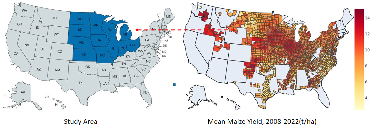
Figure 3: The figure on the left presents our study area. The figure on the right displays the yield monitor ground truth data.

2.2 Satellite data

Three VIs, including Green Chlorophyll Index (GCI) (Gitelson et al., 2005), Enhanced Vegetation Index (EVI) (Huete et al., 2002) and Normalized Difference Water Index (NDWI) (Gao, 1996), are extracted from the MODIS MCD43A4 product (Schaaf and Wang, 2015) with 500$\mathrm{m}$ spatial resolution. GCI is a metric that assesses the chlorophyll concentration in leaves, providing insight into a plant’s photosynthetic capacity. Higher values often correlate with healthier and more productive vegetation. GCI is defined as:

$$GCI=\frac{NIR}{Green}-1$$ (1)

Where $NIR$ represents the surface reflectance in the Near Infrared band, and $Green$ represents the surface reflectance in the Green band.

EVI is an enhanced vegetative index, which optimizes the vegetation signal by minimizing soil and atmosphere influences. It is particularly effective in areas with dense vegetation and provides more details about biomass and canopy structural variations:

$$EVI=2.5\times\frac{NIR-Red}{NIR+6\times Red-7.5\times Blue+1}$$ (2)

Where $Red$ and $Blue$ represent the surface reflectances of the Red band and Blue band respectively.

NDWI, the normalized water index, is used to monitor changes in water content of leaves, helping identify vegetation stress due to drought or disease. This index is particularly useful in monitoring crop condition where precise water management is crucial:

$$NDWI=\frac{NIR-SWIR}{NIR+SWIR}$$ (3)

Where $SWIR$ represents the short-wave infrared band.

2.3 Weather data

The weather observations used for the modeling experiment include daily mean air temperature (Tmean), maximum air temperature (Tmax), minimum air temperature (Tmin), maximum Vapor Pressure Deficit (VPDmax), minimum Vapor Pressure Deficit (VPDmin), and total precipitation (PPT) from the Parameter elevation Regressions on Independent Slopes Model (PRISM) dataset (Daly et al., 2015, 2008) with 4 $\mathrm{km}$ spatial resolution. Tmean represents the average air temperature over a 24-hour period. Tmax and Tmin are the highest and lowest temperature recorded in a day. VPDmax and VPDmin reflect the difference between the amount of moisture in the air and the amount it can hold when saturated. PPT indicates the total amount of rain, snow, or other precipitation falling in a given time period. Moreover, daytime and nighttime Land Surface Temperature (LSTday and LSTnight) are extracted from the MODIS MYD11A2 product (Park et al., 2005) with 1 $\mathrm{km}$ spatial resolution. LSTday and LSTnight represent the temperature of the Earth’s surface during the daylight and night hours. These meteorological features are crucial in understanding weather patterns and can have significant impacts on agricultural and environmental conditions.

2.4 Soil data

For soil properties, we use Available Water Holding Capacity (AWC), Soil Organic Matter (SOM) and Cation Exchange Capacity (CEC) from Soil Survey Geographic database (SSURGO) (USDA, ) with 30$\mathrm{m}$ spatial resolution. AWC represents the soil’s ability to hold water available for plant use, SOM is a measure of the amount of organic material present in the soil, and CEC indicates the soil’s ability to hold cations, thereby influencing soil fertility and nutrient availability.

2.5 Other data

We use the CDL mask to extract the corn field lands with 30$\mathrm{m}$ spatial resolution. On the Google Earth Engine (GEE) platform (Gorelick et al., 2017), we spatially aggregate all the RS and weather features (GCI, EVI, NDWI, LSTday, LSTnight, Tmean, Tmax, Tmin, PPT, VPDmin, VPDmax, AWC, SOM, CEC), then group them temporally to 16-day intervals from mid-May to early-October to cover the corn-growing period. The dataset spans from 2008 to 2022, including county-level historical yield records obtained from the USDA NASS (USDA, 2020). Also, our model integrates the year to grasp specific time-related features and calculates 5-year historical average yield to provide a baseline for model robustness. A total input variable length of 159 is used to train the model for county-level corn yield prediction. After all the processes, we get a dataset with approximately 600-800 bags per year and each bag is composed of 100 instances. The test set is from 2018 to 2022, while the training set ranges from 2008 to the year preceding the testing year. We set aside 20% of the training data for model validation.

3 Methodology

This paper proposes to use the attention mechanism to weight instances of the MIL for corn crop yield prediction. This section will 1) offer a comprehensive overview of our model (Sec. 3.1); 2) formally define the county-level corn yield prediction (Sec. 3.2); 3) describe the MIL and how to apply it to county-level corn yield prediction with individual pixels’ information (Sec. 3.3); 4) introduce the attention mechanism (Sec. 3.4) in detail and explain its application in our setting; 5) describe the key sampling method in MIL (Sec. 3.5).

3.1 Model overview

Our method is structured as follows (Fig. 4): We begin by applying the CDL mask to the MODIS dataset, followed by selecting specific pixels within a county and leveraging them as representative data points for learning and prediction. Next, we employ MIL to establish a many-to-one mapping. Finally, we implement an attention mechanism to assign weights to these pixels, with the expectation to assign higher weights to pure pixels and lower weights to mixed pixels.

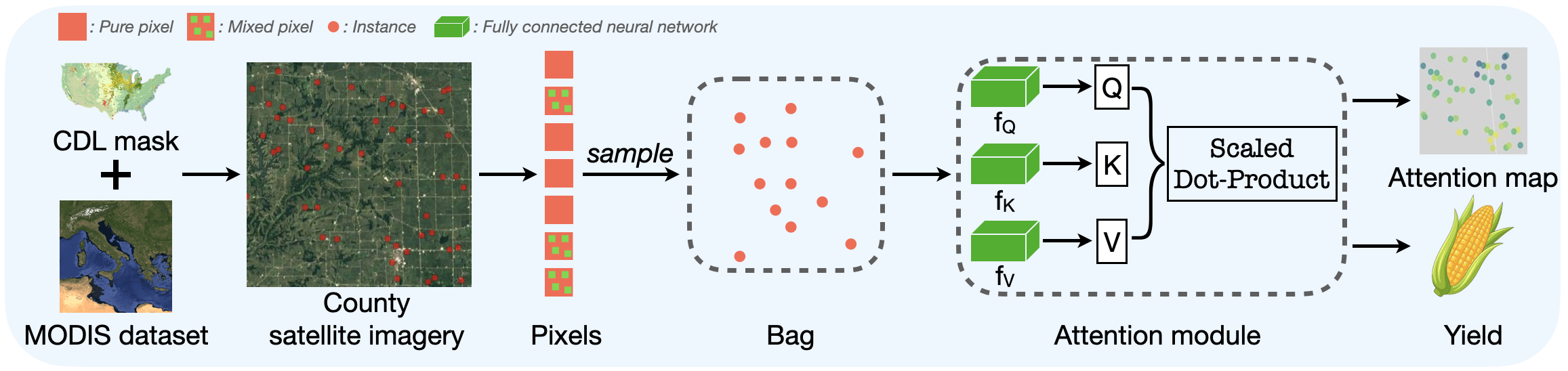
Figure 4: The pipeline of the proposed method.

3.2 Problem definition

County-level corn yield prediction process involves several key steps. First, the USDA NASS Cropland Data Layer (CDL) mask (USDA-NASS, 2017) is used to identify and extract the corn fields at 30m resolution. Subsequently, the crop field feature data sets such as vegetation Indices (VIs) derived from MODIS  (Justice et al., 1998) will be retrieved from different data sources and reprocessed, re-sampled, and reformatted to be used as modeling inputs. A machine learning model is then built based on the extracted features to predict corn yield.

To formalize the county level crop yield prediction problem, let $n$ be the number of counties in the given study area. Let $I_{i}$ be the satellite imagery and $y_{i}$ be the yield for each county $i$, $i=1,...,n$. Each image is on the space $\mathbb{R}^{W\times H\times C}$, where $W$ and $H$ are the width and height of the image, and $C$ denotes the channels. We extract some features $F_{i}$, including VIs and other agricultural environmental features (weather, soil properties, etc.) from the raw images. From a machine learning perspective, our training objective is to develop a model $f$, $f(F_{i})=y_{i}$.

3.3 Multiple instance learning

Conventional county-level corn yield prediction methods usually aggregate all the pixels in one county by some statistical methods (Ma et al., 2023b, a, 2024), which may compromise the integrity of county data representation, potentially losing some detailed information. As a response to its limitations, here we investigate pixel-level county feature processing and apply MIL to our task. In real-world applications, there are often scenarios where a single label represents a group of data points. In MIL, the above setting is described as a bag containing many instances from which we need to predict the label. For county-level corn yield prediction, we have the yield (label) of each county (bag), and each county is composed of a number of pixels (instances). By utilizing the detailed information of each county, MIL can lead to a better performance. Suppose there are $m_{i}$ pixels in each county $i$, $i=1,...,n$. For each pixel $j$, $j=1,...,m_{i}$, we extract its feature $P^{j}_{i}$. There exists a model $f$ of many-to-one mapping, namely $f(P^{1}_{i},P^{2}_{i},...,P^{m_{i}}_{i})=y_{i}$.

3.4 Attention mechanism implementation

The attention mechanism (Vaswani et al., 2017) in machine learning assigns varying importance to different input elements, enabling models to focus on inputs that are more relevant to the output (Khan et al., 2022). This helps models perform better in complex tasks by learning context-specific representations. In our task, we use attention to assign appropriate weights to the pixels in each county, anticipating that attention can automatically determine the significance of each pixel. Ideally, it assigns higher weights for pure pixels and lower weights for mixed pixels. Suppose there are $m_{i}$ pixels in county $i$, $i=1,...,n$. For the feature $P_{i}^{j}$ of pixel $j$, $j=1,...,m_{i}$, our goal is to learn a weight $W_{i}^{j}$. We are aiming for such a model $f$, $f({W^{1}_{i}}^{\top}P^{1}_{i},{W^{2}_{i}}^{\top}P^{2}_{i},...,{W^{m_{i}}_{i}}^{\top}P^{m_{i}}_{i})=y_{i}$. In this way, we can reduce as much of the noisy information in mixed pixels as possible.

The neural network learns patterns from input data through a process called forward propagation by some layers and does error adjustment with a backpropagation process (Goodfellow et al., 2016). In the attention module, we use $m_{i}$ pixels from each county $i$ and extract their features $P^{j}_{i}$ as the input vector $\breve{P_{i}}=(P^{1}_{i},P^{2}_{i},...,P^{m_{i}}_{i})$. For simplicity of notation, we omit the subscript $i$ of $\breve{P_{i}}$ here, so it becomes $\breve{P}$. Then it is passed through three separate fully connected layers $f_{Q}$, $f_{K}$, $f_{V}$ to obtain the respective vectors: query $Q$, key $K$, and value $V$.

$$Q=f_{Q}(\breve{P}),K=f_{K}(\breve{P}),V=f_{V}(\breve{P})$$ (4)

In the context of image processing, the use of query, key, and value in the attention mechanism works as follows: Query represents a specific region or aspect of the image. Key represents reference regions or elements within the image. Value contains information or features associated with each key. The mechanism calculates the similarity between the query and key, weights the values based on this similarity, and produces an output that focuses on the relevant image information. This process essentially decides which parts of the input should be paid “attention” to.

In a practical setting, we calculate the attention function on a batch of queries $Q$, keys $K$, and values $V$ concurrently, the output matrix is computed as follows:

$$Attention(Q,K,V)=softmax(\frac{QK^{\top}}{\sqrt{d_{K}}})V$$ (5)

Where $d_{K}$ is the dimension of $K$.

And The softmax function (Goodfellow et al., 2016) is defined as:

$$\text{softmax}(\mathbf{z})_{i}=\frac{e^{z_{i}}}{\sum_{j=1}^{K}e^{z_{j}}}$$ (6)

Where $\mathbf{z}=(z_{1},\dots,z_{K})$ is the input vector for $i=1,\dots,K$. $e^{z_{i}}$ is the exponential of the $i$-th element of the input vector $\mathbf{z}$.

The similarity between the query $Q$ and the key $K$ is captured through their dot product. The higher the dot product, the more similar the query $Q$ is to the key $K$. The dot product result is then passed through a softmax function to obtain the weights, which range between 0 and 1 and sum to 1. The softmax function ensures that the larger dot products get higher weights. Finally, these softmax weights are used to compute a weighted sum of the values $V$. Each value is multiplied by its corresponding weight, and these products are then summed. This final result is the output of the attention mechanism, which represents the context relevant to the query $Q$ given key-value pairs. By combining the above equations, we denote the function of our attention module as $Att(\breve{P})$, then our model $f$ becomes $f(Att(\breve{P}))=y_{i}$.

3.5 Sampling method in MIL

A key step in MIL is selecting representative instances within each bag since training on all instances in a bag is computationally expensive, especially for large bags. Additionally, without clear indications of which instances are more influential for a bag’s label, treating all instances with equal importance could potentially mislead the model during the learning process. To address this issue, Cluster-MIL (Wagstaff et al., 2008) assumes that individual items come from a group of underlying clusters, with a bag’s label being a function of one relevant cluster. The model learns the internal structure of bags that contain items from various unknown distributions. Meanwhile, Prime-MIL (Ray and Page, 2001) operates under the assumption that there exists a primary instance within each bag, then aims to select the most crucial instance for prediction. In contrast, Instance-MIL (Ray and Craven, 2005) employs each instance for regression directly, without taking the bag structure into account. In our county-level corn yield prediction task, we utilize a unique sampling method, drawing inspiration from the mixed pixel problem, to select the most representative pixels within each county. As illustrated in LABEL:fig:mixedmodis, the VIs of a CDL pixel are derived from the information of the encompassing MODIS pixel. Consequently, CDL pixels within the same MODIS pixel shares the same VIs. As a result, we randomly select one CDL pixel with cropland label from each MODIS pixel, removing the rest pixels with duplicate VIs.

Furthermore, to simplify the learning process, we need to sample an appropriate number of pixels in each county. On the one hand, selecting fewer pixels might not capture the entire information in each county. On the other hand, over-sampling may result in an insufficient number of qualified counties, making it impossible to obtain sufficient data for training. Here we randomly select 100 pixels from each county $i$, $i=1,...,n$, denoted as $\hat{P_{i}}=(P^{1}_{i},P^{2}_{i},...,P^{100}_{i})$, assuming that these selected pixels will adequately capture the county’s information. For simplicity of notation, we omit the subscript $i$ of $\hat{P_{i}}$ here, so it becomes $\hat{P}$. Ultimately, we aim to train a model $f$, $f(Att(\hat{P}))=y_{i}$ that can predict the yield accurately.

4 Experiment

The goal of crop prediction modeling is to construct a many-to-one mapping with pixel-level features as input and county-level yield as output. Features are drawn from a range of sources (Table 1), including satellite imagery, weather, and soil properties, etc. We also incorporate the year as a feature to enhance the model’s understanding of temporal patterns, and use the historical average yield to serve as a baseline to improve the model’s robustness. The extensive scope of the features will notably improve the model’s predictive power and produce more reliable results.

Category	Variables	Unit	Related Properties	Spatial Resolution	Temporal Resolution	Source	Latency
Satellite Imagery	Enhanced Vegetation Index (EVI)	N/A	Plant vigor	500$\mathrm{m}$	Daily	MODIS	One day
	Green Chlorophyll Index (GCI)
	Normalized Difference Water Index (NDWI)
	Daytime Land Surface Temperature (LSTday)	Kelvin		1$\mathrm{km}$
	Nighttime Land Surface Temperature (LSTnight)
Climate	Mean Temperature (Tmean)	${}^{\circ}C$	Heat stress	4$\mathrm{km}$		PRISM
	Max Temperature (Tmax)
	Minimum Temperature (Tmin)
	Total Precipitation (PPT)	$\mathrm{mm}$	Water stress
	maximum vapor pressure deficit (VPDmax)	$\mathrm{hPa}$
	minimum vapor pressure deficit (VPDmin)
Soil	Available Water Holding Capacity (AWC)	$\mathrm{cm}$	Soil water uptake	30$\mathrm{m}$	N/A	SSURGO	N/A
	Soil Organic Matter (SOM)	$\mathrm{kg}$/$\mathrm{m}^{2}$	Soil nutrient uptake
	Cation Exchange Capacity (CEC)	$\mathrm{cmol}$/$\mathrm{kg}$
Others	Historical average yield	t/ha	N/A	County-level		USDA NASS

Table 1: This table summarizes all the data information used in our experiments.

4.1 Experimental setup

In order to evaluate the performance of the proposed model, three popular models, including linear regression (LR) (Bishop and Nasrabadi, 2006), ridge regression (RR) (Hoerl and Kennard, 1970) and random forest (RF) (Breiman, 2001), are selected as baseline models for comparison due to their extensive application in regression tasks. In particular, LR is a statistical method predicting an outcome based on the linear relationship with one or more independent variables. Ridge regression is a variant of linear regression that adds a penalty term to prevent overfitting in high-dimensional datasets. Random forest is an ensemble machine learning algorithm that aggregates many decision trees to achieve more accurate prediction. The above three baseline models are implemented with scikit-learn (Pedregosa et al., 2011). We use the features of a county as the input and its yield as the output, conducting end-to-end training of these models. Meanwhile, to highlight the role of MIL, Instance-MIL is also included as a comparison. We use Adam (Kingma and Ba, 2014) as optimizer with batch size of $100$. Initially, the learning rate is set at $0.1$ and is reduced by a factor of 10 whenever the error reaches a plateau. All the deep learning models are developed using PyTorch (Paszke et al., 2019).

4.1.1 Performance Metrics

The experiment results are measured by standard error metrics $RMSE$ and $R^{2}$ (Albergel et al., 2013):

$$RMSE=\sqrt{\frac{\sum_{i=1}^{n}(y_{i}-\hat{y}_{i})^{2}}{n}}$$ (7)

$$R^{2}=1-\frac{\sum_{i=1}^{n}(y_{i}-\hat{y}_{i})_{2}}{\sum_{i=1}^{n}(y_{i}-\bar{y})^{2}}$$ (8)

where n is the total number of observations (counties or pixels). $y_{i}$ is the predicted value (predicted yield) for the $i\textsuperscript{th}$ observation (one pixel in RS imagery). $\hat{y}_{i}$ is the actual value (observed yield) for the $i\textsuperscript{th}$ observation. $\bar{y}$ is the mean of the observed data. The observed yield data are the official historical reports of the county level yields from USDA, NASS (USDA, 2020).

4.2 Model Performance Evaluation

The proposed model, MIL with attention mechanism (Att-MIL), is compared with other methods, including Instance-MIL without attention (Ins-MIL), LR, RR, and RF, in Table 2. The results show that our approach outperforms all other methods across all years and metrics. The superior performance of our approach can be attributed to its effective extraction and incorporation of nuanced inter-pixel correlations within each county, which other methods overlooked. A detailed analysis of the attention module is provided in the discussion section (Sec. 5). The second-best method, instance-MIL, while not incorporating attention, effectively utilizes the MIL concept, recognizing that each county consists of multiple pixels. This understanding provides a more comprehensive view than merely considering each county as a single entity and results in better performance compared to traditional regression-based methods. RF, ranking third, exhibits relatively good performance due to its robustness to noise and ability to model non-linear relationships. However, it does not inherently model detailed county information, thereby performing worse than the MIL-based methods. Linear regression and ridge regression models are based on the assumptions of linear relationships and independence among predictors, which are not entirely accurate in the context of county-level corn yield prediction. Consequently, these methods exhibit the weakest performance in our experiments. The above comparisons underscore the benefits of integrating attention mechanisms and MIL in tackling the complexity and detail-oriented nature of county-level corn yield prediction. All experimental results are obtained after averaging five repetitions. For each experiment, we randomly select different random seeds to ensure the results are fair and reproducible.

	Att		Ins		LR		Ridge		RF
	$RMSE$	$R^{2}$	$RMSE$	$R^{2}$	$RMSE$	$R^{2}$	$RMSE$	$R^{2}$	$RMSE$	$R^{2}$
2018	1.00	0.67	1.42	0.50	1.49	0.45	1.49	0.45	1.41	0.50
2019	0.99	0.58	1.18	0.51	1.46	0.26	1.45	0.27	1.60	0.10
2020	1.00	0.48	1.35	0.20	1.53	-0.02	1.81	-0.42	1.41	0.13
2021	0.99	0.64	1.16	0.60	1.78	0.05	2.04	-0.24	1.08	0.64
2022	0.83	0.84	1.07	0.73	1.35	0.65	1.18	0.73	1.19	0.73

Table 2: Model evaluation results in 2018-2022.

To illustrate the relationship between predicted and reported yields, we depict scatter plots to provide a clear visual representation of their alignment (LABEL:fig:scatter). Each point in the figures corresponds to a specific county. From these scatter plots, we observe that predictions made by Attention-MIL are tightly clustered around the line of perfect fit, indicating high accuracy. The scatter plot of instance-MIL, although less clustered than that of our method, still demonstrates a significant degree of accuracy. RF does not capture detailed information within counties, hence its results on the scatter plot are more scattered compared to the MIL-based methods. In contrast, LR and RR display the greatest spread of data points. This indicates that our approach provides more consistent and accurate results, outperforming the alternative methods presented.

Next, to visually represent the magnitude of prediction errors spatially across different regions, we present a choropleth map that illustrates the absolute error of each method across various states (LABEL:fig:abserr). The absolute error map provides a geographic representation of the prediction performance of each method at the county level. In the map, each colored block represents a county, with color intensity indicating the prediction error magnitude; deeper colors signify higher errors. Upon examination, it becomes clear that our method, which combines attention mechanism with MIL, consistently presents the lightest color across most counties. This suggests that our approach achieves the lowest absolute error overall, indicating superior prediction performance.

In comparison, the map corresponding to Instance-MIL exhibits a slightly deeper color, especially in Kansas in 2018 and in Iowa in 2020. This is because the year 2018 is particularly dry for many parts of Kansas, especially during key growth stages of the corn crop (NASS, 2018). The U.S. Drought Monitor observes part of Kansas in severe to extreme drought conditions, particularly in the earlier part of the year (Drought.gov, 2018). Furthermore, on August 10, 2020, a severe windstorm known as a “derecho” swept through Iowa (Service, 2020). This storm brought extremely high winds, with some reports of wind speeds reaching over $100mph$ in certain areas. The derecho flattened corn fields, broke plants, and caused widespread destruction to crops across the central part of the state. This event had a significant negative impact on corn yields in Iowa for 2020. We use the error map to validate the connection between the storm and prediction error ( LABEL:fig:err). For corn fields affected by the storm, the satellite imagery does not change significantly in a short period of time. As a result, machine learning models tend to overestimate the yield of those affected areas. Indeed, in 2020, the results for this region show an overestimation, which is consistent with our hypothesis. The color intensities of these blocks in the map of random forest, linear regression, and ridge regression are even deeper in Kansas and Iowa. Besides showing darker areas in the two aforementioned regions, these maps display extensive dark colors at the intersection of North Dakota, Minnesota, and South Dakota in 2021. This is because in 2021, much of the upper Midwest, including North Dakota, South Dakota, and Minnesota, experienced severe drought conditions (Drought.gov, 2021a, b, c; of Natural Resources, 2021). In particular, North Dakota also experienced higher than average temperatures during the growing season (InForum, 2021). High temperature, especially when combined with drought, can stress corn crops and reduce yields. Like storms, hot weather does not immediately affect satellite imagery, but it will impact the internal growth of plants. Therefore, high temperature can also lead to corn yield overestimation, which is confirmed in our error map ( LABEL:fig:err).

4.3 In-season yield prediction

To verify the capability of our model forproviding good prediction throughout various growth stages of corn, we conduct a comparative experiment of all models for in-season county-level corn yield prediction, dividing the timeframe from mid-May to early-October into 10 intervals, predicting once every 16 days (Fig. 6). Predicting corn yield is challenging in the initial stages of the growing season because the correlation between satellite imagery features and yield is very week (Johnson, 2014b). This experiment is based on the data in 2022 with the training data spaning from 2008 to 2021. It is clear that our method incorporating attention and MIL achieves the best $RMSE$ and $R^{2}$ values, indicating it provides the best fit to the data across all dates. In the mid-term stage of corn growth, the performance of the four methods other than Att-MIL is roughly similar. Instance-MIL performs second-best for most of the time, while Random Forest is somewhat inferior. Linear regression and ridge regression perform the worst in the early and late stages. This superior performance likely stems from MIL’s ability to manage the uncertainty and noise during the early stages of corn growth.

Figure 6: $RMSE$ and $R^{2}$ in in-season county-level corn yield prediction in 2022. The x-axis represents the test dates, while the y-axis represents the metrics.

4.4 The number of instance bags

In our experiment, a crucial parameter is the number of pixels selected from each county. Selecting too many pixels in each county may result in too few qualifying counties, thereby reducing the dataset’s size. Conversely, if the number of selected pixels is too small, these pixels may not adequately represent the complete information of a county, negatively impacting the model’s training and prediction. This naturally introduces a trade-off where more pixels in a single county leads to fewer counties being selected, and vice versa. The objective of this section is twofold: (1) identifying an optimal parameter range that allows the model to reduce space usage of the dataset without sacrificing accuracy; and (2) studying the models’ robustness under various parameter conditions. Therefore, we conduct a thorough experiment by varying the number of pixels per county between 2 and 1500 (Fig. 8). This experiment is launched based on the test set from 2018 to 2022, while the training set ranges from 2008 to the year preceding the testing year. Finally, we show the mean value of results from 2018 to 2022.

Figure 8: This figure depicts the $RMSE$ and $R^{2}$ when the number of sampled pixels in each county changes.

As shown in Fig. 8, our model consistently demonstrates superior performance, while the instance-MIL and random forest models exhibit poorer performance across all conditions. Meanwhile, Linear regression and ridge regression, perform substantially worse as the number of counties decreases, despite the increased number of pixels per county. This might be attributed to the inability of these models to generalize well over smaller datasets. Notably, even as the number of counties decreases, our model’s predictive performance remains robust.

In addition, the results suggest a suitable range of pixel number spanning from 100 to 1000. Within this range, the predictions of our Attention-MIL model exhibit minimal fluctuation, with the optimal outcome achieved at 100 pixels. These findings highlight the effectiveness and robustness of our approach, particularly in scenarios with limited data. This implies that our model is well-suited for handling datasets of varying sizes, demonstrating a significant advantage in real-world county-level corn yield predictions.

5 Discussion

This section provides a detailed analysis of the origins and functions of attention mechanism. In Sec. 5.1, we calculate some necessary data and perform data preprocessing. Next we pose two important questions regarding the attention mechanism (Sec. 5.2). In Sec. 5.3 and Sec. 5.4, we delve into a deep analysis of attention by answering the two proposed questions. We then select a few counties as examples, magnifying their satellite images to demonstrate the role of attention ( Sec. 5.5). Finally, we summarize the advantages of attention in Sec. 5.6.

5.1 Pixel mixing level calculation and preprocessing

To explore the role of attention, we first need to quantify the mixed pixels based on their definition, which is the proportion of the crop field within a pixel in the feature dataset. Taking the MODIS dataset as an example, suppose one MODIS pixel contains $n$ CDL pixels. We represent each MODIS pixel as a binary list $S$ of length $n$, where each element $s_{i}$ represents a CDL pixel, $s_{i}\in\{0,1\}$ for $i=1,2,...,n$. Then we can calculate corn ratio, which is the number of CDL pixels contained within a MODIS pixel by GEE, as the ground truth for our experiment:

$$corn\>ratio=\frac{\Sigma_{i=1}^{n}s_{i}}{n}$$ (9)

For the following analysis, the initial step of preprocessing is “bag normalization” by normalizing the corn ratio within each bag so that the sum of corn ratio in each bag equals one. Suppose we select $m$ pixels in each county $i$, $i=1,...,n$. In county $i$ We have a corn ratio $C_{i}^{j}$ for each pixel $j$, $j=1,...,m$. Then the implementation of bag normalization is as follows:

$${C_{i}^{j}}^{\prime}=\frac{C_{i}^{j}}{\Sigma_{k=1}^{m}C_{i}^{k}}$$ (10)

Where ${C_{i}^{j}}^{\prime}$ is bag-normalized corn ratio.

The purpose of bag normalization is to make attention and corn ratio comparable. We first normalize the corn ratio values within each bag, transforming them into relative values. This ensures the fairness of subsequent experiments.

5.2 Attention analysis

In the above experiments, we demonstrate that Attention-MIL can indeed enhance the predictive ability of the model. However, to ascertain the specific role that attention plays within the model, further in-depth analysis is necessary. We need to answer two questions: (1) How does the model learn attention, and which part of input contributes the most? and (2) Do the weights learned by the attention mechanism truly reflect the degree of mixing in each pixel? In this section, we will demonstrate the specific function of attention by analyzing the relationship between attention, features, and corn ratio. This experiment is based on the data in 2022 with the training data spaning from 2008 to 2021.

5.3 Attention’s correlation with features

5.3.1 Feature importance

To answer the first question, examining the importance of feature is essential as we can verify if the model derives attention based on relatively important features (Khan et al., 2022). To investigate feature importance, we employ the feature ablation strategy (Litkowski, 2016). For each feature, we retrain our model after excluding that feature to test its impact on the model’s performance (Table 3). In this way, we can infer that if there’s a notable decline in performance when a feature is removed. This indicates the feature’s crucial significance.

	SOM	Year	CEC	PPT	VPDmin	VPDmax	Tmin	LSTnight
RMSE	0.848	0.865	0.875	0.889	0.901	0.928	0.934	0.954
$R^{2}$	0.832	0.829	0.829	0.818	0.814	0.814	0.809	0.799

	AWC	Tmean	NDWI	EVI	LSTday	GCI	Tmax	Historical
RMSE	0.975	0.992	1.003	1.024	1.051	1.059	1.062	1.130
$R^{2}$	0.790	0.789	0.784	0.783	0.780	0.777	0.774	0.759

Table 3: This table displays the results of our feature ablation experiments.

Through this examination, we found the descending order of feature importance to be as follows: historical average yield, Tmax, GCI, LSTday, EVI, NDWI, Tmean, AWC, LSTnight, Tmin, VPDmax, VPDmin, PPT, CEC, year, and SOM (Fig. 9). The historical average yield is considered as 100% importance, and the least important feature SOM is treated as 0% importance. The most important feature, historical average yield, suggests that past yield data is crucial in predicting future yields. This is aligned with the notion that past performance can often provide a strong baseline for future prediction. Tmax and GCI rank high, implying the importance of temperature and vegetation health on corn yield. On the other hand, the relatively low importance of features like year and SOM indicates these features, while having some predictive power, contribute less significantly compared to other more impactful features. We rank the importance of features here to delve deeper into their relationship with attention in subsequent analyses (Sec. 5.3.2).

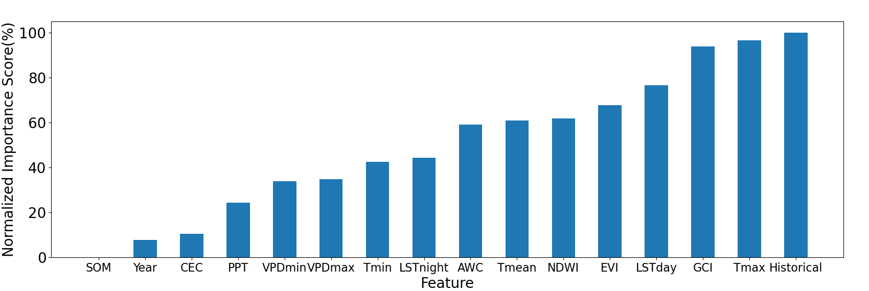
Figure 9: This figure displays the normalized importance ranking of a total of 16 features.

5.3.2 Correlation results

Since our model’s input consists of various features, we aim to understand how the model learns attention from these features by using the Pearson correlation coefficient (Freedman et al., 2007). The Pearson correlation coefficient quantifies the linear relationship between two continuous variables. We identify some of the most important features in the feature importance experiment, and explore how the model learns attention by calculating the correlation coefficients between these features and attention. We perform the same pre-processing “bag normalization” as in Sec. 5.1 to make it into relative value.

As displayed in the Table 4, the results indicate that attention has a high correlation with several important features, such as VIs, LSTday, and Tmax. Since we know that the function of attention is to learn the part of the input that has a higher correlation with the output, we can conclude that the attention mechanism obtains attention scores by learning those important features.

Variables	NDWI	GCI	EVI	LSTday	Tmax	Corn ratio
Correlation	0.50	0.53	0.48	0.45	0.52	0.68

Table 4: The Pearson correlation coefficient between attention with some of the most important features and corn ratio.

5.4 Attention’s correlation with corn ratio

To answer the second question, we explore if attention truly reflects the degree of mixing in mixed pixels, thereby assigning the correct weights to these pixels. Our goal is to empirically demonstrate the connection between attention and corn ratio. As displayed in the Table 4, the results suggest a high correlation between attention score and corn ratio, indicating that our attention accurately predicts the degree of mixing in the mixed pixels.

5.5 Zoomed-in mixed and pure pixels analysis

Previous experiments validate the role of attention, corn ratio, and features from a statistical perspective. Now we delve into each county and pixel to visually examine their connection (LABEL:fig:zoom) by selecting four counties from all the data as examples to demonstrate the effect of attention from top to bottom. From left to right, the figures represent attention, corn ratio, a zoomed-in view of a pure pixel, and a zoomed-in view of a mixed pixel.

First, we analyze the county-level attention visualization results from a macro perspective. In LABEL:fig:zoom (a), we observe that the top left corner contains a group of darker-colored pure pixels, while the top right corner has a set of lighter-colored mixed pixels. This pattern corresponds well with our attention and corn ratio. Similarly, in LABEL:fig:zoom (b), we can see that the pixels in the center are darker, while those on the right are lighter. In LABEL:fig:zoom (c), the left half of the pixels appear darker, and the upper right section has lighter-colored pixels. In LABEL:fig:zoom (d), the bottom left and top right portions of the pixels are darker, while the diagonal section from the top left to the bottom right is lighter. These patterns clearly demonstrate the correlation between our attention and corn ratio at the county-level.

Next, we zoom in the clusters of the mixed pixels and pure pixels to validate the aforementioned analysis. It is observed that in the pure pixels, all the land is planted to the corn category, while in the mixed pixels, a significant portion of the land is occupied by unrelated categories like forests. This fully demonstrates that our attention captures the information of the mixed cropland.

5.6 Attention’s advantage over corn ratio

It is observed that the correlation between attention and corn ratio is not perfect 100%. The first reason is the inherent errors coming from the calculation of the corn ratio. This is attributed to the datasets’ pixel sizes not being perfectly divisible and the boundaries of various pixels not matching up seamlessly. As illustrated in the LABEL:fig:mixedmodis, the edges of the MODIS pixel do not align perfectly with the edges of the smaller CDL pixels. This results in numerous CDL pixels at the periphery that are only partially contained within MODIS pixels. When we count these CDL pixels for calucating the corn ratio, it leads to inaccuracy. Therefore, we allow the model to automatically learn attention, as we argue that the attention derived in this way will be more accurate and reliable.

The second reason is that our attention is a learned weight from all features. In the above experiment, we calculate the corn ratio solely based on the MODIS dataset, introducing certain errors. Therefore, our attention module provides a more comprehensive result compared to calculated corn ratio.

6 Conclusion

This paper explores county-level corn yield prediction by viewing each county as a collection of corn fields containing multiple pixels. First, MIL is employed to leverage the pixel-level RS observations, balance the conflict between computational resources and information integrity, and address the lack of finer-grained yield records for pixel-level data processing. Subsequently, to tackle the mixed pixel problem caused by inconsistent resolutions among feature datasets and crop mask, an attention mechanism is incorporated to assign weights to pixels, thereby enhancing prediction accuracy. We analyze the role of attention from both statistical and micro perspectives, confirming the validity of our approach. In the future, we will endeavor to enhance the generalization of the model by transfer learning for larger-scale corn yield prediction research. Additionally, we aim to adapt our model for utilization in diverse crop types and geographic regions.

References

- Albergel et al. (2013) Albergel, C., Brocca, L., Wagner, W., de Rosnay, P., Calvet, J.C., 2013. Selection of performance metrics for global soil moisture products: The case of ascat product. Remote Sensing of Energy Fluxes and Soil Moisture Content 427.
- Bastiaanssen and Ali (2003) Bastiaanssen, W.G., Ali, S., 2003. A new crop yield forecasting model based on satellite measurements applied across the indus basin, pakistan. Agriculture, ecosystems & environment 94, 321–340.
- Battude et al. (2016) Battude, M., Al Bitar, A., Morin, D., Cros, J., Huc, M., Sicre, C.M., Le Dantec, V., Demarez, V., 2016. Estimating maize biomass and yield over large areas using high spatial and temporal resolution sentinel-2 like remote sensing data. Remote Sensing of Environment 184, 668–681.
- Bishop and Nasrabadi (2006) Bishop, C.M., Nasrabadi, N.M., 2006. Pattern recognition and machine learning. volume 4. Springer.
- Breiman (2001) Breiman, L., 2001. Random forests. Machine learning 45, 5–32.
- Carbonneau et al. (2018) Carbonneau, M.A., Cheplygina, V., Granger, E., Gagnon, G., 2018. Multiple instance learning: A survey of problem characteristics and applications. Pattern Recognition 77, 329–353.
- Daly et al. (2008) Daly, C., Halbleib, M., Smith, J.I., Gibson, W.P., Doggett, M.K., Taylor, G.H., Curtis, J., Pasteris, P.P., 2008. Physiographically sensitive mapping of climatological temperature and precipitation across the conterminous united states. International Journal of Climatology: a Journal of the Royal Meteorological Society 28, 2031–2064.
- Daly et al. (2015) Daly, C., Smith, J.I., Olson, K.V., 2015. Mapping atmospheric moisture climatologies across the conterminous united states. PloS one 10, e0141140.
- Deines et al. (2021) Deines, J.M., Patel, R., Liang, S.Z., Dado, W., Lobell, D.B., 2021. A million kernels of truth: Insights into scalable satellite maize yield mapping and yield gap analysis from an extensive ground dataset in the us corn belt. Remote sensing of environment 253, 112174.
- Dietterich et al. (1997) Dietterich, T.G., Lathrop, R.H., Lozano-Pérez, T., 1997. Solving the multiple instance problem with axis-parallel rectangles. Artificial intelligence 89, 31–71.
- Drought.gov (2018) Drought.gov, 2018. Historical drought conditions in kansas. https://www.drought.gov/states/kansas.
- Drought.gov (2021a) Drought.gov, 2021a. Historical drought conditions for north dakota. https://www.drought.gov/states/north-dakota.
- Drought.gov (2021b) Drought.gov, 2021b. Historical drought conditions for south dakota. https://www.drought.gov/states/south-dakota.
- Drought.gov (2021c) Drought.gov, 2021c. Historical drought conditions in minnesota. https://www.drought.gov/states/minnesota.
- Freedman et al. (2007) Freedman, D., Pisani, R., Purves, R., 2007. Statistics (international student edition). Pisani, R. Purves, 4th edn. WW Norton & Company, New York .
- Gao (1996) Gao, B.C., 1996. Ndwi—a normalized difference water index for remote sensing of vegetation liquid water from space. Remote sensing of environment 58, 257–266.
- Gitelson et al. (2005) Gitelson, A.A., Viña, A., Ciganda, V., Rundquist, D.C., Arkebauer, T.J., 2005. Remote estimation of canopy chlorophyll content in crops. Geophysical research letters 32.
- Goodfellow et al. (2016) Goodfellow, I., Bengio, Y., Courville, A., 2016. Deep learning. MIT press.
- Gorelick et al. (2017) Gorelick, N., Hancher, M., Dixon, M., Ilyushchenko, S., Thau, D., Moore, R., 2017. Google earth engine: Planetary-scale geospatial analysis for everyone. Remote Sensing of Environment URL: https://doi.org/10.1016/j.rse.2017.06.031, doi:10.1016/j.rse.2017.06.031.
- Haykin (1998) Haykin, S., 1998. Neural networks: a comprehensive foundation. Prentice Hall PTR.
- Hoerl and Kennard (1970) Hoerl, A.E., Kennard, R.W., 1970. Ridge regression: Biased estimation for nonorthogonal problems. Technometrics 12, 55–67.
- Hu et al. (2023) Hu, H., Ye, R., Thiyagalingam, J., Coenen, F., Su, J., 2023. Triple-kernel gated attention-based multiple instance learning with contrastive learning for medical image analysis. Applied Intelligence , 1–16.
- Huang et al. (2015) Huang, J., Ma, H., Su, W., Zhang, X., Huang, Y., Fan, J., Wu, W., 2015. Jointly assimilating modis lai and et products into the swap model for winter wheat yield estimation. IEEE Journal of Selected Topics in Applied Earth Observations and Remote Sensing 8, 4060–4071.
- Huete et al. (2002) Huete, A., Didan, K., Miura, T., Rodriguez, E.P., Gao, X., Ferreira, L.G., 2002. Overview of the radiometric and biophysical performance of the modis vegetation indices. Remote sensing of environment 83, 195–213.
- Ilse et al. (2018) Ilse, M., Tomczak, J., Welling, M., 2018. Attention-based deep multiple instance learning, in: International conference on machine learning, PMLR. pp. 2127–2136.
- InForum (2021) InForum, 2021. 2021 was north dakota’s 5th warmest year on record. https://www.inforum.com/news/north-dakota/2021-was-north-dakotas-5th-warmest-year-on-record.
- Jin et al. (2019) Jin, Z., Azzari, G., You, C., Di Tommaso, S., Aston, S., Burke, M., Lobell, D.B., 2019. Smallholder maize area and yield mapping at national scales with google earth engine. Remote Sensing of Environment 228, 115–128.
- Johnson (2014a) Johnson, D.M., 2014a. An assessment of pre-and within-season remotely sensed variables for forecasting corn and soybean yields in the united states. Remote Sensing of Environment 141, 116–128.
- Johnson (2014b) Johnson, D.M., 2014b. An assessment of pre-and within-season remotely sensed variables for forecasting corn and soybean yields in the united states. Remote Sensing of Environment 141, 116–128.
- Justice et al. (1998) Justice, C.O., Vermote, E., Townshend, J.R., Defries, R., Roy, D.P., Hall, D.K., Salomonson, V.V., Privette, J.L., Riggs, G., Strahler, A., et al., 1998. The moderate resolution imaging spectroradiometer (modis): Land remote sensing for global change research. IEEE transactions on geoscience and remote sensing 36, 1228–1249.
- Khaki and Wang (2019) Khaki, S., Wang, L., 2019. Crop yield prediction using deep neural networks. Frontiers in plant science 10, 621.
- Khaki et al. (2020) Khaki, S., Wang, L., Archontoulis, S.V., 2020. A cnn-rnn framework for crop yield prediction. Frontiers in Plant Science 10, 1750.
- Khan et al. (2022) Khan, S., Naseer, M., Hayat, M., Zamir, S.W., Khan, F.S., Shah, M., 2022. Transformers in vision: A survey. ACM computing surveys (CSUR) 54, 1–41.
- Kingma and Ba (2014) Kingma, D.P., Ba, J., 2014. Adam: A method for stochastic optimization. arXiv preprint arXiv:1412.6980 .
- LeCun et al. (1995) LeCun, Y., Bengio, Y., et al., 1995. Convolutional networks for images, speech, and time series. The handbook of brain theory and neural networks 3361, 1995.
- Litkowski (2016) Litkowski, K., 2016. Feature ablation for preposition disambiguation. Damascus, MD, USA: CL Research .
- Liu et al. (2022) Liu, Y., Wang, S., Chen, J., Chen, B., Wang, X., Hao, D., Sun, L., 2022. Rice yield prediction and model interpretation based on satellite and climatic indicators using a transformer method. Remote Sensing 14, 5045.
- Lobell and Burke (2010) Lobell, D.B., Burke, M.B., 2010. On the use of statistical models to predict crop yield responses to climate change. Agricultural and forest meteorology 150, 1443–1452.
- Ma et al. (2024) Ma, Y., Chen, S., Ermon, S., Lobell, D.B., 2024. Transfer learning in environmental remote sensing. Remote Sensing of Environment 301, 113924. URL: https://www.sciencedirect.com/science/article/pii/S0034425723004765, doi:https://doi.org/10.1016/j.rse.2023.113924.
- Ma et al. (2019) Ma, Y., Kang, Y., Ozdogan, M., Zhang, Z., 2019. County-level corn yield prediction using deep transfer learning, in: AGU Fall Meeting Abstracts, pp. B54D–02.
- Ma et al. (2023a) Ma, Y., Yang, Z., Huang, Q., Zhang, Z., 2023a. Improving the transferability of deep learning models for crop yield prediction: A partial domain adaptation approach. Remote Sensing 15, 4562.
- Ma et al. (2023b) Ma, Y., Yang, Z., Zhang, Z., 2023b. Multisource maximum predictor discrepancy for unsupervised domain adaptation on corn yield prediction. IEEE Transactions on Geoscience and Remote Sensing 61, 1–15.
- Ma and Zhang (2022) Ma, Y., Zhang, Z., 2022. Multi-source unsupervised domain adaptation on corn yield prediction, in: AI for Agriculture and Food Systems.
- Ma et al. (2021a) Ma, Y., Zhang, Z., Kang, Y., Özdoğan, M., 2021a. Corn yield prediction and uncertainty analysis based on remotely sensed variables using a bayesian neural network approach. Remote Sensing of Environment 259, 112408.
- Ma et al. (2021b) Ma, Y., Zhang, Z., Yang, H.L., Yang, Z., 2021b. An adaptive adversarial domain adaptation approach for corn yield prediction. Computers and Electronics in Agriculture 187, 106314.
- Mishra et al. (2013) Mishra, V., Cruise, J.F., Mecikalski, J.R., Hain, C.R., Anderson, M.C., 2013. A remote-sensing driven tool for estimating crop stress and yields. Remote Sensing 5, 3331–3356.
- NASS (2018) NASS, U., 2018. Usda nass 2018 kansas corn statistics. https://kscorn.com/2019/02/08/usda-nass-2018-kansas-corn-statistics/.
- of Natural Resources (2021) of Natural Resources, M.D., 2021. The drought of 2021. https://www.dnr.state.mn.us/climate/journal/drought-2021.html.
- Nevavuori et al. (2019) Nevavuori, P., Narra, N., Lipping, T., 2019. Crop yield prediction with deep convolutional neural networks. Computers and electronics in agriculture 163, 104859.
- Park et al. (2005) Park, S., Feddema, J., Egbert, S., 2005. Modis land surface temperature composite data and their relationships with climatic water budget factors in the central great plains. International Journal of Remote Sensing 26, 1127–1144.
- Paszke et al. (2019) Paszke, A., Gross, S., Massa, F., Lerer, A., Bradbury, J., Chanan, G., Killeen, T., Lin, Z., Gimelshein, N., Antiga, L., et al., 2019. Pytorch: An imperative style, high-performance deep learning library. Advances in neural information processing systems 32.
- Pedregosa et al. (2011) Pedregosa, F., Varoquaux, G., Gramfort, A., Michel, V., Thirion, B., Grisel, O., Blondel, M., Prettenhofer, P., Weiss, R., Dubourg, V., Vanderplas, J., Passos, A., Cournapeau, D., Brucher, M., Perrot, M., Duchesnay, E., 2011. Scikit-learn: Machine learning in Python. Journal of Machine Learning Research 12, 2825–2830.
- Ray and Craven (2005) Ray, S., Craven, M., 2005. Supervised versus multiple instance learning: An empirical comparison, in: Proceedings of the 22nd international conference on Machine learning, pp. 697–704.
- Ray and Page (2001) Ray, S., Page, D., 2001. Multiple instance regression, in: Brodley, C.E., Danyluk, A.P. (Eds.), Proceedings of the Eighteenth International Conference on Machine Learning (ICML 2001), Williams College, Williamstown, MA, USA, June 28 - July 1, 2001, Morgan Kaufmann. pp. 425–432.
- Rumelhart et al. (1985) Rumelhart, D.E., Hinton, G.E., Williams, R.J., et al., 1985. Learning internal representations by error propagation.
- Rymarczyk et al. (2021) Rymarczyk, D., Borowa, A., Tabor, J., Zielinski, B., 2021. Kernel self-attention for weakly-supervised image classification using deep multiple instance learning, in: Proceedings of the IEEE/CVF Winter Conference on Applications of Computer Vision, pp. 1721–1730.
- Sakamoto et al. (2013) Sakamoto, T., Gitelson, A.A., Arkebauer, T.J., 2013. Modis-based corn grain yield estimation model incorporating crop phenology information. Remote Sensing of Environment 131, 215–231.
- Sakamoto et al. (2014) Sakamoto, T., Gitelson, A.A., Arkebauer, T.J., 2014. Near real-time prediction of us corn yields based on time-series modis data. Remote Sensing of Environment 147, 219–231.
- Schaaf and Wang (2015) Schaaf, C., Wang, Z., 2015. Mcd43a4 modis/terra+ aqua brdf/albedo nadir brdf adjusted ref daily l3 global-500m v006. nasa eosdis land processes daac. USGS Earth Resources Observation and Science (EROS) Center, Sioux Falls, South Dakota (https://lpdaac. usgs. gov) .
- Service (2020) Service, N.W., 2020. August 10, 2020 derecho. https://www.weather.gov/dmx/2020derecho.
- Shahhosseini et al. (2021) Shahhosseini, M., Hu, G., Huber, I., Archontoulis, S.V., 2021. Coupling machine learning and crop modeling improves crop yield prediction in the us corn belt. Scientific reports 11, 1606.
- Shuai and Basso (2022) Shuai, G., Basso, B., 2022. Subfield maize yield prediction improves when in-season crop water deficit is included in remote sensing imagery-based models. Remote Sensing of Environment 272, 112938.
- (63) USDA, . Soil survey staff, natural resources conservation service, united states department of agriculture. web soil survey. available online at https://websoilsurvey.nrcs.usda.gov/. accessed [12/06/2020] .
- USDA (2020) USDA, 2020. United states department of agriculture national agricultural statistics service .
- USDA-NASS (2017) USDA-NASS, C., 2017. Usda national agricultural statistics service cropland data layer .
- Vaswani et al. (2017) Vaswani, A., Shazeer, N., Parmar, N., Uszkoreit, J., Jones, L., Gomez, A.N., Kaiser, Ł., Polosukhin, I., 2017. Attention is all you need. Advances in neural information processing systems 30.
- Wagstaff et al. (2008) Wagstaff, K.L., Lane, T., Roper, A., 2008. Multiple-instance regression with structured data, in: 2008 IEEE international conference on data mining workshops, IEEE. pp. 291–300.
- Wang et al. (2020) Wang, X., Huang, J., Feng, Q., Yin, D., 2020. Winter wheat yield prediction at county level and uncertainty analysis in main wheat-producing regions of china with deep learning approaches. Remote Sensing 12, 1744.
- Xu et al. (2005) Xu, M., Watanachaturaporn, P., Varshney, P.K., Arora, M.K., 2005. Decision tree regression for soft classification of remote sensing data. Remote Sensing of Environment 97, 322–336.
- Yang et al. (2021) Yang, Y., Anderson, M.C., Gao, F., Johnson, D.M., Yang, Y., Sun, L., Dulaney, W., Hain, C.R., Otkin, J.A., Prueger, J., et al., 2021. Phenological corrections to a field-scale, et-based crop stress indicator: An application to yield forecasting across the us corn belt. Remote Sensing of Environment 257, 112337.