Scaling Whole-Chip QAOA for Higher-Order Ising Spin Glass Models on Heavy-Hex Graphs

Abstract

We show through numerical simulation that the Quantum Alternating Operator Ansatz (QAOA) for higher-order, random-coefficient, heavy-hex compatible spin glass Ising models has strong parameter concentration across problem sizes from $16$ up to $127$ qubits for $p=1$ up to $p=5$, which allows for straight-forward transfer learning of QAOA angles on instance sizes where exhaustive grid-search is prohibitive even for $p>1$. We use Matrix Product State (MPS) simulation at different bond dimensions to obtain confidence in these results, and we obtain the optimal solutions to these combinatorial optimization problems using CPLEX. In order to assess the ability of current noisy quantum hardware to exploit such parameter concentration, we execute short-depth QAOA circuits (with a CNOT depth of 6 per $p$, resulting in circuits which contain $1420$ two qubit gates for $127$ qubit $p=5$ QAOA) on $100$ higher-order (cubic term) Ising models on IBM quantum superconducting processors with $16,27,127$ qubits using QAOA angles learned from a single $16$-qubit instance. We show that (i) the best quantum processors generally find lower energy solutions up to $p=3$ for 27 qubit systems and up to $p=2$ for 127 qubit systems and are overcome by noise at higher values of $p$, (ii) the best quantum processors find mean energies that are about a factor of two off from the noise-free numerical simulation results. Additional insights from our experiments are that large performance differences exist among different quantum processors even of the same generation and that dynamical decoupling significantly improve performance for some, but decrease performance for other quantum processors. Lastly we show $p=1$ QAOA angle mean energy landscapes computed using up to a $414$ qubit quantum computer, showing that the mean QAOA energy landscapes remain very similar as the problem size changes.

1 Introduction

The Quantum Alternating Operator Ansatz (QAOA) [1], and the predecessor Quantum Approximate Optimization Algorithm [2, 3], is a quantum algorithm that is intended to be a heuristic solver of combinatorial optimization problems. QAOA is typically considered to be a variational hybrid quantum-classical algorithm because there is a set of parameters (usually called angles) that must be tuned in order for QAOA to perform well - and typically the standard tuning approach is to use a classical processor to perform iterative gradient descent learning on the QAOA angles, using the quantum computer to evaluate the expectation value of the algorithm at a different angles. The motivation for this approach, typically, is that because quantum computers are very difficult to engineer to have low error rate gate operations, current technologies have fairly high error rates - but by using variational algorithms, part of the computation can be off-loaded onto the classical part of the computation. Unfortunately, the task of learning good QAOA angles (and learning variational parameters for hybrid quantum-classical algorithms in general), is computationally hard and only made harder by the presence of noise in the quantum computation [4, 5]. For these reasons, the suitability of QAOA for Noisy Intermediate-Scale Quantum (NISQ) [6] computers is unclear, and is being actively studied using a variety of different approached [7, 8, 9, 10, 11, 12, 13].

The Quantum Alternating Operator Ansatz consists of the following components: an initial state $\ket{\psi}$, a phase separating cost Hamiltonian $H_{C}$, a mixing Hamiltonian $H_{M}$ (here the standard transverse field mixer $H_{M}=\sum_{i=1}^{N}\sigma^{x}_{i}$), a number of rounds $p\geq 1$ to apply $H_{C}$ and $H_{M}$ (also referred to as the number of layers), and two real vectors of angles $\vec{\gamma}=(\gamma_{1},...,\gamma_{p})$ and $\vec{\beta}=(\beta_{1},...,\beta_{p})$, each with length $p$.

There exist a large number of QAOA variants because there are a variety of choices of initial states, phase separating cost Hamiltonians (for many different combinatorial optimization problems), mixer Hamiltonians, and tuning methods for the QAOA angles [14, 15, 16, 17, 18, 19]. The central question of all QAOA variants is how will QAOA scale in terms of obtaining optimal solutions of combinatorial optimization problems as the number of variables increases. This question has different components, including the angle finding problem, how many $p$ rounds need to be applied in order to be competitive with existing classical methods, and how the algorithm performs as problem size increases. It is known that in general, reasonably high $p$ (e.g. more than $p=1$ or $p=2$) will need to be applied in order for QAOA to be perform well at solving combinatorial optimization problems [20, 21, 22, 23, 24]. For this reason, the task of increasing $p$ on larger problem sizes is of particular interest, and this is the primary question that is studied in this paper, using state of the art quantum computing hardware.

Using the whole-chip heavy-hex tailored QAOA circuits that are targeting hardware-compatible Ising models proposed in Refs. [25, 26], we investigate the task of scaling these QAOA circuits to higher rounds, and to larger heavy-hex chip quantum processors. Notably, this class of random spin glasses contain higher order terms, which increases the problem difficulty, and can be natively addressed by QAOA. The primary challenge with implementing these extremely large QAOA circuits up to higher $p$ is the angle finding task. Refs. [25, 26], utilized the brute-force approach of full angle gridsearches on the quantum hardware in order to compute good angles for $p=1$ and $p=2$. Unfortunately, this approach scales exponentially with $p$ if the grid resolution is held constant and in practice on-device angle gridsearch learning with $p=3$ is already computationally prohibitive. Refs. [25, 26] observed that problem instances of the same sizes, but with different random coefficient choices, had nearly-identical low-round QAOA energy landscapes. Our approach in this study to overcoming these angle finding challenges is to make use of parameter concentration in QAOA angles in order to transfer high-quality fixed angles from small ($16$ qubit instances) to larger instances. Parameter concentration has been observed analytically and numerically for a number of different QAOA problem types [27, 22, 28, 29, 30, 31, 12, 32, 33, 25, 26].

The goal of this study is to investigate the ideal scaling of QAOA on current quantum computing hardware (with respect to increasing $p$ and increasing the number of variables), using the largest problem sizes that can be feasibly programmed on the hardware. This study uses two critical components:

1. The angle-finding procedure is not performed in a variational outer loop classical optimization procedure, but we rather rely on heuristically computed good QAOA angles found on smaller problem instances and then apply transfer learning. The angle-finding technique with quantum hardware in the inner loop has been studied before on NISQ hardware [11, 10], but there are a number of limitations with making this technique feasible – including the computational overhead of the angle learning due to challenges such as local minima, and the noise in the computation making the learning task more difficult. Ideally, good QAOA angles would be able to be computed off-chip (classically), and then be used on large-scale quantum hardware. This is what the transfer learning has enabled us to do for qubit system sizes that cannot be addressed using brute-force computation.

2. Because of the relatively high error rates on the current quantum computers, implementing optimization problems whose structure matches the underlying hardware graph reduces the overhead of gate-depth and gate-count. In particular, on quantum processors that have a sparse hardware graph, implementing long range interactions can be quite costly in terms of SWAP gates. Therefore, defining the combinatorial optimization problems that we sample to be compatible with the IBM Quantum processor heavy-hex graph [25, 26] allows the QAOA circuits to be extremely short depth.

We briefly describe our methods and approach in Section 2 by giving a description of the higher-order Ising (minimization) optimization problems (Subsection 2.1), the QAOA circuits to sample these optimization problems (Subsection 2.2); we describe the angle finding and parameter transfer methods (Subsection 2.3), and give a brief description of the Matrix Product State (MPS) simulation methods (Subsection 2.4) and the use of CPLEX to classically find the optimal solutions to the optimization problems (Subsection 2.1). Lastly, the implementation details on IBM quantum computers are given in Subsection 2.5.

In Section 3, the first set of results shows (Subsection 3.1) parameter transfer works very well for these classes of problems up to $p=5$ in a noise-free environment as we show through numerical simulation for up-to $127$ qubits, when trained only on a single 16-qubit instance. In particular, mean expectation values improve consistently with increasing $p$ for all of 100 randomly chosen problem instances at 16, 27, and 127 qubits. These results are enabled by classical simulation techniques. As these problem classes grow entanglement relatively slowly grows with increasing $p$, MPS simulations enable us to classically produce the solution distributions that QAOA would achieve on an error-corrected quantum computer for up to $p=5$ and $127$ qubits. Our confidence in the accuracy of these simulations is due to the convergence of the solution values as we increase the MPS bond dimension parameter. Having established that parameter transfer works in a noise-free computation, we then examine to what extent parameter transfer works on actual NISQ computers.

In a second set of results (Subsection 3.2), we execute the $100$ problem instances (for each qubit count) on cloud-accessed IBM quantum processors with $16$, $27$, and $127$ qubits using the numerically obtained fixed angles from a single $16$ qubit instance. We find the following:

1. Performance varies significantly among different processors even if they are from the same hardware generation. For the $127$ qubit devices, the best expectation values (with respect to $p$) and averaged over all 100 instances varies from $-45$ to $-80$ with the noise-free value of $-160$. For the 27 qubit quantum computers, the range is from $-8$ to $-16$ with the noise free value at $-28$. Thus, the noise in the computation impacts solution quality significantly.

2. The digital dynamical decoupling sequences we evaluated (pairs of Pauli X gates) improved the performance of three out of four 127 qubit devices, two out of six 27-qubit devices, and the single 16 qubit device.

3. Averaged over 100 instances, the best 127 qubit processors improve until $p=2$ and start degrading at higher values of $p$. For 27 qubits, the best processors improve up to $p=3$. Thus, noise appears to effect the higher qubit count devices slightly more than lower qubit count devices despite equal CNOT depth at the same $p$.

Overall, our second set of results shows that QAOA parameter transfer works for our class of problems on quantum processors albeit we can only verify up to $p=3$ as the devices succumb to noise at larger $p$. We thus revisit the question of parameter transferability on quantum hardware in a more systematic fashion in a third set of results limited to $p=1$. We find that parameter concentration remains stable even if trained on actual quantum hardware. We show mean energy QAOA angle landscapes for the two parameters at $p=1$ for four different 27 qubit and one 414 qubit systems (Subsection 3.3) that all look nearly identical. For the 127-qubit backends, we show that best solution distributions are of similar shape on different backends but shifted linearly to account for better average expectation values (Subsection 3.3).

2 Methods

First we outline the hardware-compatible combinatorial optimization problems in Subsection 2.1. The QAOA algorithm is described in Subsection 2.2; Subsection 2.3 describes the optimized angle-finding and transfer learning procedure that allows high-quality angles to be computed for $127$-qubit QAOA circuits, and Subsection 2.4 describes the MPS simulations. Lastly, Subsection 2.5 describes the hardware implementation.

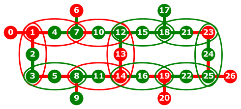
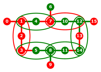
Figure 1: Examples of higher order Ising models that are hardware-compatible with a heavy-hex hardware graph: (left) A $27$-qubit device: Nodes correspond to linear terms, edges to quadratic terms, and hyperedges encircling three neighboring nodes to cubic terms. Ising coefficients of $-1$ and $+1$ are depicted in red and green, respectively. (right) A $16$-qubit device: Illustrating the terminology of Equation (1), we have $W=\{2,4,5,10,11,13\}$, with the remaining nodes in $V_{2}$ being $V_{2}\setminus W=\{0,6,9,15\}$. For node $4\in W$, we have neighbors $\{n_{1}(l),n_{2}(l)\}=\{1,7\}\subset V_{3}$. (bottom) A $127$-qubit device: Higher order Ising model comprised of $127$ linear, $144$ quadratic and $71$ cubic terms.

2.1 Heavy-Hex Compatible Ising Models

The class of minimization combinatorial optimization problems that we consider are heavy-hex graph native spin glasses, and were introduced and described in Refs. [25, 26]. This class of models was designed specifically to be heavily optimized for a heavy-hex hardware graph [34], and can include higher order terms (specifically cubic terms), thus making the optimization problem more difficult. Importantly, although Refs. [25, 26] used these problems for sampling $127$ qubit heavy-hex native problems, this problem type is well defined for any heavy-hex hardware graph size. Here, we consider random instances of these problem types defined on $16$, $27$, $127$, and $414$ qubit IBM Quantum hardware graphs.

For a heavy-hex graph $G=(V,E)$ and a vector of spins $z=(z_{0},\ldots,z_{n-1})\in\{+1,-1\}^{n}$ we define a cost function

$$C(z)=\sum_{v\in V}d_{v}\cdot z_{v}+\sum_{(i,j)\in E}d_{i,j}\cdot z_{i}\cdot z_{j}+\sum_{l\in W}d_{l,n_{1}(l),n_{2}(l)}\cdot z_{l}\cdot z_{n_{1}(l)}\cdot z_{n_{2}(l)},$$ (1)

and a QAOA cost Hamiltonian $H_{C}$ by replacing spin variables $z_{i}$ with Pauli operators $\sigma_{z}^{i}$. Equation (1) defines a random spin glass problem with specific cubic terms: Any subgraph of a heavy-hex lattice is a bipartite graph with vertices $V=\{0,\ldots,n-1\}$ is uniquely bipartitioned as $V=V_{2}\sqcup V_{3}$ with $E\subset V_{2}\times V_{3}$, where $V_{i}$ consists of vertices of maximum degree $i$. $W$ is the set of vertices $l\in V_{2}$ of exactly equal to $2$, with neighbors denoted by $n_{1}(l)$ and $n_{2}(l)$, see Figure 1. Thus $d_{v}$, $d_{i,j}$, and $d_{l,n_{1}(l),n_{2}(l)}$ are the linear, quadratic and cubic coefficients, respectively. The coefficients are chosen randomly from $\{+1,-1\}$ with probability $0.5$, see Figure 1. Figure 1 (bottom) shows an example problem instance defined on a $127$ qubit heavy-hex graph.

Instance generation and assessment

In Table 1, we give a summary of the studied hardware devices as well as the problem instances generated to run on these QPUs. For each group of QPUs sharing the same hardware graph, we generate 100 random problem instances according to Equation (1), which are shared across these devices.

One additional problem type we evaluate on a subset of the hardware experiments is Equation (1) without cubic terms, i.e., random spin glass problems with only linear and quadratic terms. To assess the achieved QAOA performances in context, we additionally compute for each instance the minimum (ground state) energy and the maximum energy. This is done with CPLEX [35] after a preprocessing with order reductions, as outlined in Ref. [26].

	Hardware					#Instance Coefficients
Device name	Processor	#Qubits	#2q-Gates	Basis gates		linear	quadratic	cubic
ibm_seattle	Osprey r1	414	475	ECR,	ID, RZ, SX, X	414	475	232
ibm_washington	Eagle r1	127	142	CX,	ID, RZ, SX, X	127	142	69
ibm_sherbrooke	Eagle r3	127	144	ECR,	ID, RZ, SX, X	127	144	71
ibm_brisbane	Eagle r3	127	144	ECR,	ID, RZ, SX, X	127	144	71
ibm_cusco	Eagle r3	127	144	ECR,	ID, RZ, SX, X	127	144	71
ibm_nazca	Eagle r3	127	144	ECR,	ID, RZ, SX, X	127	144	71
ibm_geneva	Falcon r8	27	28	CX,	ID, RZ, SX, X	27	28	11
ibm_auckland	Falcon r5.11	27	28	CX,	ID, RZ, SX, X	27	28	11
ibm_algiers	Falcon r5.11	27	28	CX,	ID, RZ, SX, X	27	28	11
ibmq_kolkata	Falcon r5.11	27	28	CX,	ID, RZ, SX, X	27	28	11
ibmq_mumbai	Falcon r5.10	27	28	CX,	ID, RZ, SX, X	27	28	11
ibm_cairo	Falcon r5.11	27	28	CX,	ID, RZ, SX, X	27	28	11
ibm_hanoi	Falcon r5.11	27	28	CX,	ID, RZ, SX, X	27	28	11
ibmq_guadalupe	Falcon r4P	16	16	CX,	ID, RZ, SX, X	16	16	6

Table 1: QPU and Instance summary. Numbers of available qubits and 2-qubit gates are accurate at the time in which the experiments of this study were executed. Devices mainly differ in their native 2-qubit gates (ECR vs. CX), and in the ratios between the numbers of linear, quadratic and cubic instance coefficients that can be accommodated.

2.2 Whole Chip QAOA Circuit Description

The Quantum Alternating Operator Ansatz consists of preparing the initial state $\ket{\psi}$, then for $p$ rounds applying alternatingly the phase separating Hamiltonian $H_{C}$ for time $\gamma_{i}$ and the mixing Hamiltonian $H_{M}$ for time $\beta_{i}$:

$$\ket{\vec{\gamma},\vec{\beta}}=\underbrace{e^{-i\beta_{p}H_{M}}e^{-i\gamma_{p}H_{C}}}_{\text{round }p}\cdots\underbrace{e^{-i\beta_{1}H_{M}}e^{-i\gamma_{1}H_{C}}}_{\text{round }1}\ket{\psi}$$ (2)

In each round, $H_{C}$ is first applied which separates out the basis states of the state vector by phases $e^{-i\gamma C(z)}$. Next, $H_{M}$ gives parameterized interference between solutions with different cost values. After $p$ rounds, the state $\ket{\vec{\gamma},\vec{\beta}}$ is measured in the computational basis and thus finds a sample $z$ of cost value $C(z)$ with probability $|\braket{z}{\vec{\gamma},\vec{\beta}}|^{2}$. Notably, the QAOA cost Hamiltonian can include higher order polynomial terms [36, 37], without requiring ancilla qubit overhead. We make use of this property of QAOA in order to sample higher-order Ising models that are heavy-hex hardware-compatible, introduced in Refs. [25, 26].

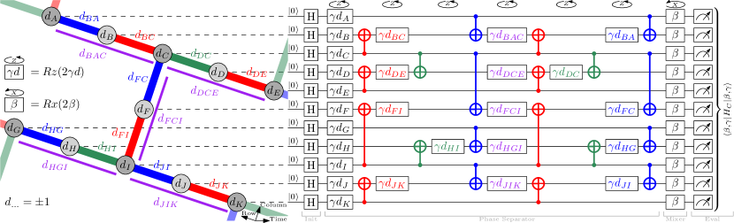
Figure 2: From Refs. [25, 26]: QAOA circuit description for heavy-hex graph compatible higher order Ising models of arbitrary size. The graph is bipartite and has an arbitrary 3-edge-coloring given by Kőnig’s line coloring theorem. (left) 3-edge-coloring and bipartite grey-shading of the nodes. Adjacent purple lines denote the cubic terms terms. (right) Any quadratic term (colored edge) gives rise to a combination of two CNOTs and a Rz-rotation in the phase separator, giving a CNOT depth of 6 due to the degree-3 nodes. When targeting the degree-2 nodes with the CNOT gates, these constructions can be nested to implement the cubic terms with just one additional Rz-rotation.

Figure 2 shows the QAOA circuit construction algorithm used in this study for one layer of the algorithm ($p=1$) which is the same for all layers, specifically targeting the Ising model type defined in Equation (1). The transverse field mixer QAOA implementation is used in all circuits. A greedy Breadth-first search (BFS) 3-edge-coloring is computed each time a circuit is constructed, and that same edge coloring is then used for all $p$ layers in that circuit.

The operators $e^{-i\beta H_{M}}$ and $e^{-i\gamma H_{C}}$ are $2\pi$-periodic, hence we can restrict the QAOA angle search space to $\beta_{i},\gamma_{i}\in[0,2\pi)$ for each round $1\leq i\leq p$. However, careful consideration of the parity of solution values as well as symmetries when starting in the state $\ket{\psi}=\ket{+^{n}}$ and measuring in the computational basis allows us to further restrict the search space to $\beta_{1},\ldots,\beta_{p-1}\in[0,\pi)$, $\beta_{p}\in[0,\tfrac{\pi}{2})$, and $\gamma_{1},\ldots,\gamma_{p}\in[0,\pi)$, see Ref. [26].

2.3 QAOA angle finding with JuliQAOA and Transfer Learning

Arguably the most difficult aspect of implementing most variants of QAOA is determining good angles. Specifically, it is known that in general QAOA needs to be applied for a reasonably high number of rounds ($p$) [20, 21] in order to get to high quality solutions of combinatorial optimization problems. However, this requires high quality angles (since in almost all cases there are no analytical solutions for optimal QAOA angles) for each $p$, and there are a total of $2p$ angles that need to be optimized. The standard variational hybrid quantum-classical approach to this is to repeatedly evaluate the expectation value of the cost Hamiltonian $H_{C}$ for different sets of angles on a quantum computer, using a classical algorithm to guide exploration in angle space. This approach is quite costly however with respect to total compute time. Moreover, because current quantum computers are quite noisy, learning good angles in this manner is in general hard, and in particular are infeasible for a $127$ qubit instance. A promising approach to mitigate some of these problems is to find good angles on smaller, more tractable instances and then use those same angles on larger instances. This technique, often referred to as parameter transfer or parameter concentration, has been shown to be effective, both analytically and numerically, for a number of different problem types [27, 22, 28, 29, 30, 31, 12, 32, 33, 25, 26]. Motivated by the existing evidence for parameter transfer working for different problem sizes, and by the experimental evidence for parameter concentration across different random heavy-hex native Ising models observed in [25, 26], we utilize parameter transfer in order to obtain good fixed angles for this class of random Ising models with higher order terms. Specifically, we obtain good angles for $p=1,2,3,4,5$ on a single random $16$ qubit instance, and then validate that those angles transfer to other random $16$ qubit instances, and random $27$ qubit, as well as random $127$ qubit instances. These angles are not optimal QAOA angles, rather they are high-quality heuristic angles, in particular meaning that we obtain reliable improvements in the mean energy as a function of $p$ increasing.

The method we use to compute these good angles is the high-performance, QAOA-specific quantum simulator JuliQAOA [38]. This allows us to find very high quality angles, in this case running $O(10^{5})$ exact statevector simulations on one $16$ qubit instance (derived from the ibmq_guadalupe architecture) with higher order terms for $p=1,\ldots,5$. JuliQAOA has been used in several previous QAOA publications, with the goal of computing very high quality QAOA angles on general types of combinatorial optimization problems [39, 8, 24, 16]. The fixed angles used for the experiments shown in Subsection 3.2 are given explicitly in Appendix A.

2.4 MPS simulations

We use MPS formalism to compute approximations to $\ket{\vec{\gamma},\vec{\beta}}$ in Equation (2). Specifically, a version of time-evolving block decimation [40] has been used to simulate the action of $e^{-i\gamma_{k}H_{C}}$ and $e^{-i\beta_{k}H_{M}}$ for $k=1,\ldots,p$. MPS tensors are ordered in the same way as the qubits are labeled in Figure 1. The accuracy of MPS simulations is determined by bond dimension, denoted by $\chi$ here. In general, the accuracy is improved with growing $\chi$. Significant portion of the terms in $e^{-i\gamma_{k}H_{C}}$ are non-local and accurate simulation with MPS requires the bond dimension to grow quickly. The terms $e^{-ih_{\alpha}}$ in $e^{-i\gamma_{k}H_{C}}$ can be naturally grouped together, so all $h_{\alpha}$ are three-body. Each $e^{-ih_{\alpha}}$ can be written as Matrix Product Operator with bond dimension 2. This means that exact simulation of $e^{-ih_{\alpha}}$ can increase the MPS bond dimension by at most factor of 2, for some MPS tensors. Therefore, simulations with small $p$ can be performed exactly and accuracy will gradually deteriorate as $p$ is increased.

We perform MPS simulations with $\chi=2^{m}$, for $m=4,\ldots,11$ to estimate the impact of errors. The summary of our results is presented in Figure 3. All the panels show the error in the energy $\Delta E$ as a function of bond dimension. It is measured as $\Delta E=|E_{\chi}-E_{2048}|$, where $E_{\chi}=\bra{\psi^{\mathrm{MPS}}_{\chi}}H_{C}\ket{\psi^{\mathrm{MPS}}_{\chi}}$. Here, $\ket{\psi^{\mathrm{MPS}}_{\chi}}$ is an MPS approximation to $\ket{\vec{\gamma},\vec{\beta}}$ in Equation (2) obtained by a simulation with maximum bond dimension of $\chi$. Our most accurate simulations are performed with $\chi=2048$, and hence we treat $E_{2048}$ as the best approximation to the exact energy. Solid, black lines in Figure 3 represent $\Delta E$ averaged over one hundred instances of $H_{C}$. All simulation errors, for all instances of $H_{C}$, are within gray areas shown in Figure 3.

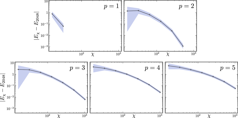
Figure 3: Error analysis performed for MPS simulations. Here we show error in the energy $|E_{\chi}-E_{2048}|$ as a function of bond dimension $\chi$ for different values of $p$. Solid black lines represent the error in the energy averaged over one hundred instances of $H_{C}$. All computed errors, for all instances, are contained within gray areas around black lines. The gray areas are relatively small, especially at large $\chi$. This indicates that different instances of $H_{C}$ result in similar errors. Errors are small; they are all below $0.1$, which is observed in the hardest case of $p=5$. Simulations with $p<5$ incur smaller errors.

MPS simulations become exact for $p=1$ and $p=2$ at $\chi=64$ and $\chi=1024$ respectively. As pointed out above, the proper treatment of $e^{-i\gamma_{k}H_{C}}$ allows us to perform exact simulations at relatively small values of $\chi$. The error $\Delta E$ drops to zero in those cases. Those values are not shown in $p=1$ and $p=2$ panels of Figure 3. Simulations with $p>2$ are no longer exact but the errors are small and do not exceed $0.1$ for $p=5$. Note that $\Delta E$ is an absolute error in the energy. In relative terms, the error is below $10^{-3}$, given $E_{2048}\approx-150$ on average. It is important to note that all simulation errors, for all instances of $H_{C}$ are similar to each other, especially in the large $\chi$ limit. This is indicated by very thin gray error areas around the mean values of the error in all panels. Our error analysis strongly suggests that our MPS simulation is dependable and sufficiently accurate (for considered values of $p$) to represent results that would have been obtained on a quantum computer in the limit of vanishingly small noise.

Since MPS is a unitary tensor network, one can draw bitstrings $z$ from the probability distribution $P(z)=|\braket{z}{\psi^{\mathrm{MPS}}_{\chi}}|^{2}$ [41]. That is, one can approximately calculate samples that would have been drawn from $\ket{\vec{\gamma},\vec{\beta}}$ in Equation (2), assuming that the quantum computer has been executing operations noiselessly. We use that fact to generate samples shown in Figure 5.

On average, computing $\ket{\psi^{\mathrm{MPS}}_{\chi}}$ for $p=5$ and $\chi=2048$ took less than $1.5$ hour on a 48-core computational node.

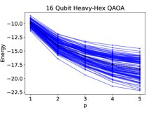
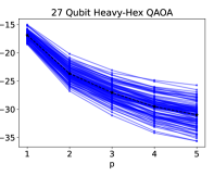
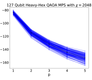
Figure 4: Classical simulations of mean energies demonstrating (noiseless) concentration of QAOA parameters. We simulate 100 random instances for each circuit size using fixed QAOA angles (trained on a single 16 qubit instance):(left) The angles for $1\leq p\leq 5$ are used to execute QAOA on 100 random 16-qubit higher-order heavy-hex instances,(center) The same angles are used for 100 random $27$-qubit instances, (right) MPS simulation with bond dimension $\chi=2048$ is used for 100 random $127$-qubit instances. For growing circuit size $16,27,127$, for every random higher-order Ising model, as $p$ increases the mean energy strictly improves, showing that transfer learning succeeds in a noiseless setting. In each plot, also the mean energy across the instance ensemble is plotted as a dashed black line.

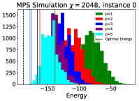
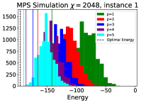
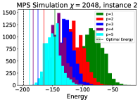
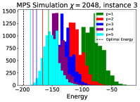
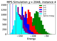
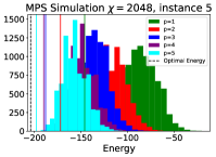
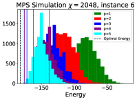
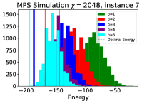
Figure 5: MPS simulation sample distributions, using a bond dimension of $\chi=2048$ for $127$-qubit QAOA circuits sampling eight of the higher-order Ising model problem instances. For each $p$, a total of $8192$ samples are computed. The ground state energy is marked in all plots with a dashed vertical black line, and the minimum energy found within each $p$ energy distribution is marked with a vertical solid line. In addition to the means of the distributions improving as a function of $p$ (shown for all $100$ problem instances in Figure 4), we see here that the minimum energy sampled also improves as $p$ increases. Notably, none of the distributions sampled the optimal energy, although the minimum energies from $p=4$ and $p=5$ are close to the optimal energy. These distributions show the ideal QAOA sampling capabilities, using the classical simulation method of MPS, if the quantum computation was noiseless.

2.5 IBM Quantum Hardware Implementation Details

The quantum circuits are passed through the Qiskit [42] transpiler in order to adapt the circuits to the hardware native gateset, such as adapting the circuits to use the two qubit unidirectional echoed cross-resonance ECR [43] gate. The QAOA circuits are heavily optimized for the heavy-hex hardware graph, so the compilation uses the fixed hardware graph and the compiler optimization is not able to reduce the two qubit gate count.

We also evaluate a relatively simple, and hardware gate-native, digital dynamical decoupling scheme of pulses of pairs of Pauli X gates, scheduled both As Soon As Possible (ASAP) and As Late As Possible (ALAP). This is implemented in Qiskit using the digital dynamical decoupling pass [44]. Dynamical decoupling is an open loop quantum control error suppression technique for mitigating decoherence on idle qubits [45, 46, 47, 48, 49], which can be approximated using digital sequences of single qubit gates that are mathematically equivalent to applying the identity gate. Appendix B contains detailed compiled circuit renderings for $p=1$ whole-chip $127$ qubit QAOA circuits.

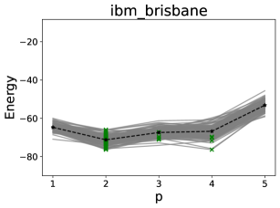
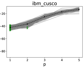
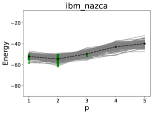
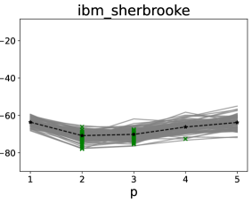
Figure 6: Mean experimental QAOA energies of 100 hardware-compatible instances without dynamical decoupling: Each grey line is an instance shared across devices with experiments run for $p=1,2,3,4,5$. Each green ‘$\times$’ marker gives the $p$ that achieves lowest mean energy for the corresponding instance. The black dashed line shows the average mean QAOA energy across all 100 random spin glass instances with cubic terms. Each data point is computed from 20,000 shots on a 127-qubit device. For each $p$, angles are fixed across all devices and instances.

3 Results

Subsection 3.1 presents numerical simulations showing that under noiseless conditions QAOA parameter transfer works well, and can be applied to significantly larger problem sizes than what was trained on. Subsection 3.2 then uses these fixed angles to execute QAOA circuits on a variety of IBM Quantum hardware. Subsection 3.3 presents a low $p$ comparison between $127$ qubit quantum processors, showing a clear improvement on newer generations of IBM quantum computers. Subsection 3.3 show $p=1$ QAOA energy landscapes, on whole-chip higher order Ising models, computed on various IBM quantum computers with qubit counts ranging from $27$ qubits up to $414$ qubits showing consistent parameter transfer as the problem sizes increase but the energy landscapes remain relatively unchanged.

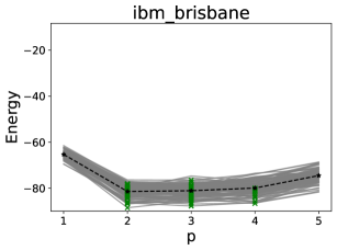
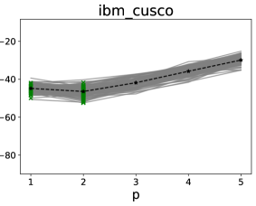
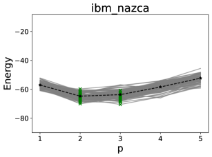
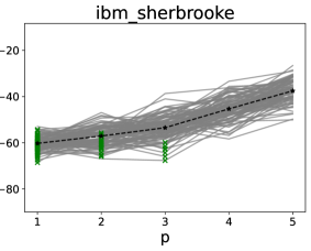
Figure 7: Mean experimental QAOA energies of 100 random instances with ALAP-scheduled dynamical decoupling: Each grey line is an instance shared across devices; each green ‘$\times$’ marker gives its corresponding $p$ that achieves lowest mean energy. The black dashed line shows the average mean QAOA energy across all instances. Cf. Figure 6.

3.1 Numerical Simulations of Transfer Learning of QAOA Angles

As introduced in Subsection 2.3, parameter concentration is the following property of a QAOA problem: QAOA parameter (angle) values that are optimized for a single instance $I$ of a particular combinatorial optimization problem (such as random spin glasses or Maximum Cut) are transferable to other instances of similar structure, but potentially of significantly different size from the original $I$. Parameters from an instance $I$ are transferable to an instance $I^{\prime}$ if the quality of the solutions found by QAOA are similar for both $I$ and $I^{\prime}$. While more formal definitions of transferability are possible, we pragmatically define that parameters transfer from $I$ to $I^{\prime}$ up to a maximum number of rounds $p_{\max}$ if the mean solution quality for both $I$ and $I^{\prime}$ improves with increasing number of rounds $p$ up to and including $p_{\max}$. Figure 4 presents the numerical simulation results for the scaling of increasing $p$ QAOA using the fixed parameter transfer angles on $100$ random ensembles for $16$, $27$, and $127$ qubit instances, using the methods described in Subsection 2.3. Specifically, the same $\vec{\beta},\vec{\gamma}$ (for each $p$) are used for all numerical simulations in these plots (Appendix A explicitly gives what these fixed angles are). The $16$ and $27$ qubit data is the mean energy taken from $10,000$ samples per circuit with no noise model, simulated classically using Qiskit [42]. Simulations of 127-qubit system are performed with MPS. Here we quote expectation values of $H_{C}$ computed by direct tensor contraction. That computation is equivalent to the limit of infinite number of shots. Figure 4 shows that the transfer learning succeeded, and in particular allows us to obtain good angles for up to $p=5$, verified by classical MPS simulations. Figure 3 studies the errors in MPS simulations for all $100$ random $127$ qubit hardware-compatible instances, as a function of $\chi$, including the largest QAOA circuit depth we tested (which is $p=5$). Figure 5 shows distributions of samples for the QAOA circuits, computed using the MPS simulation method (with a bond dimension of $\chi=2048$), which shows what the expected performance of QAOA is under noiseless conditions, for a subset of the $127$ variable problem instances.

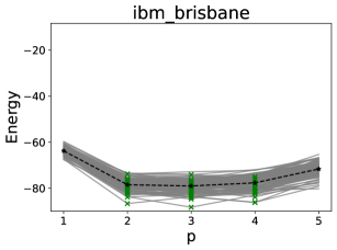
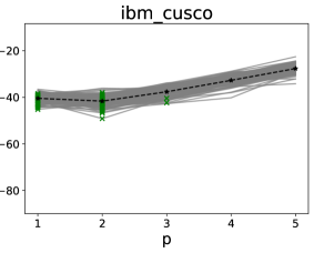
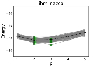
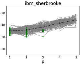
Figure 8: Mean experimental QAOA energies of 100 random instances with ASAP-scheduled dynamical decoupling: Each grey line is an instance shared across devices; each green ‘$\times$’ marker gives its corresponding $p$ that achieves lowest mean energy. The black dashed line shows the average mean QAOA energy across all instances. Cf. Figure 6.

3.2 Scaling $p$ on 16, 27, and 127 qubit IBM Quantum Processor Hardware

The results presented in this section are reported as the mean energy of the samples of the problem Ising models, from a total of $20,000$ shots per parameter and device. The plots in this section use the angles learned from a $16$ qubit instance, giving good approximation ratios as $p$ increases for the ideal computation. Figure 4 in Subsection 3.1 shows the scaling in $p$ under noiseless conditions obtained with these angles. In particular, these numerical simulations show that in the noiseless setting we would get improving energy for each step of $p$. In this section, we execute the whole-chip QAOA circuits on various IBM Quantum computers, specifically using the fixed angles discussed in Subsection 3.1 for $p=1$ up to $p=5$. This is therefore an evaluation of how well the transfer-learned angles perform on the heavy-hex graph hardware.

The bare QAOA circuits results are plotted in Figure 6 for four 127 qubit backends and Figure 9 for six 27 qubit devices and a single 16 qubit device (ibmq_guadelupe. Recall that without noise, these figures would look identical to the corresponding plots from Figure 4. Figures 7 and 10 show the hardware-executed mean energy for the QAOA circuits using ALAP-scheduled dynamical decoupling QAOA circuits for the 127 and 27 qubit systems respectively. Figures 8 and 11 show the same, but with ASAP-scheduled digital dynamical decoupling sequences.

For the 127 qubit device from Figure 6, we see that NISQ reality does indeed look different: As a first observation, three out of four quantum processors (ibm_brisbane,ibm_nazca,ibm_sherbrooke)at least improve the mean energy as averaged over the 100 instances until $p=2$, as indicated by the black dashed line, but fail to improve for higher $p$, due to noise. The green crosses indicate for each instances the $p$ at which the minimum was achieved; we see that some instances are actually optimized at $p=3,4$ or also $p=1$ for a few of the instances. The remaining backend ibm_cusco performs best at $p=1$. Secondly, despite all backends featuring an Eagle r3 QPU, performance differences are significant with ibm_brisbane achieving best average energies of almost -70 and ibm_cusco only achieving about -42. Overall, these differences are consistent with the reported two-qubit gate fidelities for these devices. For a third observation, we compare to the noise-free results from Figure 4, which show that the average energies across the instances should be roughly $-85,-110,-130,-140,-145$ for $p=1,2,3,4,5$ respectively. The actual achieved best values are at best $-70$, thus noise negatively impacts these results at all $p$ values.

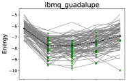
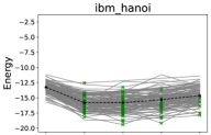
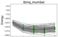
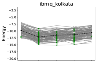
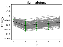
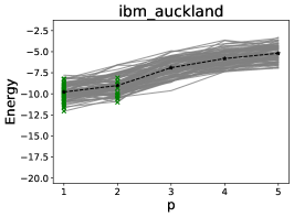
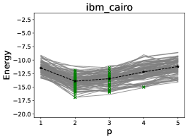
Figure 9: Mean energy of the samples measured from the whole-chip QAOA circuits, without dynamical decoupling: Each grey line is an instance run for $1\leq p\leq 5$, with its green ‘$\times$’ marker the $p$ that achieves lowest mean energy. The black dashed line shows the average mean QAOA energy taken across all 100 random higher-order instances. Each data point is computed from 20,000 shots. The same $100$ problem instances were executed on a total of six $27$-qubit devices, and $100$ $16$-qubit instances were executed on ibmq_guadalupe; with angles shared for any given $p$.

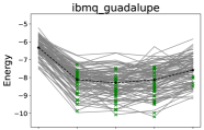
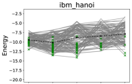
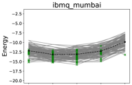
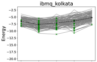
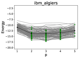
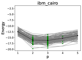
Figure 10: Mean energy of the samples from the QAOA circuits run with ALAP-scheduled dynamical decoupling: Each grey line is an instance run for $1\leq p\leq 5$, with its green ‘$\times$’ marker the $p$ that achieves lowest mean energy. The black dashed line shows the average mean QAOA energy taken across all 100 random instances. Cf. Figure 9.

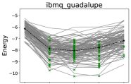
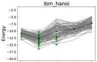
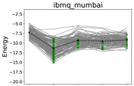
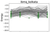
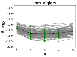
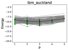
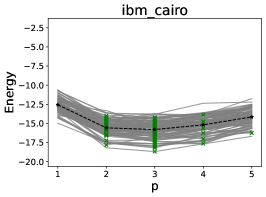
Figure 11: Mean energy of the samples from the QAOA circuits run with ASAP-scheduled dynamical decoupling: Each grey line is an instance run for $1\leq p\leq 5$, with its green ‘$\times$’ marker the $p$ that achieves lowest mean energy. The black dashed line shows the average mean QAOA energy taken across all 100 random instances. Cf. Figure 9.

In a fourth observation, we look at the two corresponding 127 qubit plots with digital dynamical decoupling sequences, i.e., Figure 7 for ALAP, and Figure 8 for ASAP. Overall, the two different schemes seem to perform similar. However, both ALAP and ASAP have a positive effect on the performance of three of the backends: ibm_brisbane improves to nearly $-80$ values and almost achieves a minimum at $p=3$ instead of at $p=2$, but not quite. The two lower performing backends ibm_cusco and ibm_nazca also see significant improvements. Strikingly, however, ibm_sherbrooke’s performance takes a significant hit with both ALAP and ASAP.

Our observations are similar for the 16 and 27 qubit systems from Figure 9: While most backends still have their average minimum performance at $p=2$, in most cases many instances find their minimum at $p=3$. ibmq_mumbai is a laudable exception as it reaches the minimum average at $p=3$ and in fact remains nearly flat even to $p=4$. Secondly, we again see performance difference among the 27 qubit systems ranging from $-16$ for ibmq_mumbai to a $-10$ value for ibm_auckland, which actually achieves its minimum at $p=1$. Thirdly, the average noise-free energies across the instances should be roughly $-17,-23,-25,-27,-30$ for $p=1,2,3,4,5$ respectively, from Figure 4, compared to the best achieved values of about $-16$; thus noise is an issue even at these lower qubit counts.

Our fourth observation with respect to dynamical decoupling for the 27 qubit backends (see Figure 11 and Figure  10) is less optimistic than for the 127 qubit count: dynamical decoupling only helps two out of six backends, namely ibm_algiers and ibm_cairo, which actually matches ibmq_mumbai’s performance without dynamical decoupling. ASAP-scheduled digital dynamical decoupling shows an average increase of the mean energy up to $p=3$ for ibm_auckland albeit at relatively poor performance. The 16 qubit backend ibmq_guadalupe profits from dynamical decoupling with a minimum mean energy up to $p=3$.

Appendix E contains tables (Table 2 and Table 3) showing the exact optimal energy for all $300$ fixed higher-order problem instances studied in this section, along with the minimum energies sampled across the QAOA circuits when executed on hardware. The tables also include the maximum energies of the problem instances, which gives a quantification of the range of the energy spectrum of these higher order Ising models. Notably, these tables show that the IBM Quantum processors were able to find the optimal solution with at least one sample for the $27$ and $16$ variable problem instances, but were never able to find the optimal solution to the $127$ variable problem instances.

3.3 $p=1$ QAOA Hardware Angle Gridsearch Results

$414$ qubit $p=1$ QAOA on ibm_seattle:

Figure 12 shows $p=1$ angle gridsearch on ibm_seattle for a random Ising model instance with cubic terms and without cubic terms. The angle gridsearch is presented in terms of the mean energy computed from the distribution of $10,000$ samples drawn for each $\beta_{1},\gamma_{1}$ angle. A total of $7,200$ linearly spaced $\beta_{1},\gamma_{1}$ are evaluated, as in Refs. [25, 26]. The higher order Ising model is comprised of $475$ quadratic terms, $414$ linear terms, and $232$ ZZZ terms (e.g. hyperedges). The Ising model with no higher order terms is comprised of $475$ quadratic terms and $414$ linear terms.

Notably, the hardware-computed $p=1$ energy landscape on these $414$ qubit instances are very similar to the $p=1$ energy landscapes shown in Ref. [26]. Figure 13 shows the full energy distribution (of $10,000$ samples) for the best $p=1$ angles on the hardware-gridsearch, along with the optimal energy. Note that the minimum energies found from the $p=1$ sampling are far away from the optimal solution energy.

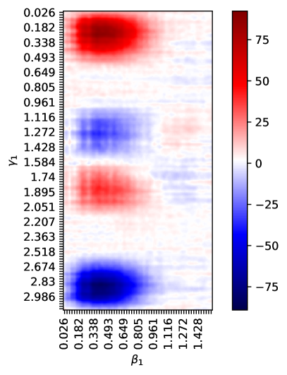
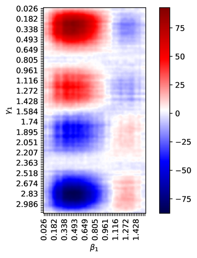
Figure 12: Experimental mean energy landscapes for a $p=1$ QAOA on ibm_seattle for two 414 qubit instances: (left) A higher-order Ising model with up to cubic terms. (right) An Ising model with linear and quadratic terms.

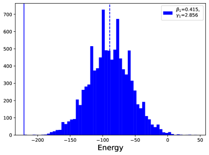
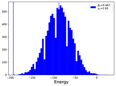
Figure 13: Experimental sample energy distribution for a $p=1$ QAOA on ibm_seattle for two 414 qubit instances, for optimal angles found in the hardware angle gridsearch that minimize the mean energy (shown in Figure 12): (left) The higher-order model with cubic terms, with a mean energy of $-89.14$ for angles $\beta=0.415,\ \gamma=2.856$. (right) The model with linear and quadratic terms, with a mean energy of $-87.72$ for angles $\beta=0.467,\ \gamma=2.83$. The mean energies are marked with vertical dashed blue lines. The vertical solid lines mark the minimum sample energy found among the 10,000 samples at these angles; however, during the whole angle gridsearch, the overall mininum sample energies lie at $-241$ for the higher-order Ising model and $-221$ for the Ising model on the right.
For context, the energy spectra of the instances range from $-637$ (ground state) to $+623$ (maximum) for the higher-order model on the left and from $-567$ (ground state) to $+565$ (maximum) for the Ising model on the right.

$27$ qubit $p=1$ gridsearch:

Figure 14 shows hardware $p=1$ angle gridsearch mean energy heatmaps on several IBM Quantum processors. Notably, the energy landscapes are very similar to the $414$ qubit whole-lattice heavy-hex QAOA in Subsection 3.3, and the previously reported $127$ qubit whole-lattice heavy-hex QAOA results from Ref. [26]. Notice that the energy landscape from ibm_geneva is considerably more noisy compared to the other device energy heatmaps.

Comparison of difference 127 qubit IBMQ Processors with Whole-Chip $p=1$ QAOA Circuits:

A straightforward question that can be asked using whole-chip circuits is how different processors compare, when executing the same circuit. This offers a clear way to benchmark device performance, using all available hardware components. In this section, we use the short depth QAOA circuits to compare three of the $127$ qubit IBM Quantum superconducting qubit processors; ibm_washington, ibm_brisbane, and ibm_sherbrooke. We do this using a focused QAOA angle gridsearch for $p=1$ QAOA depth, using higher order Ising models that are compatible with all three of these processors - which in particular means hardware compatible with ibm_washington, as its hardware graph is a subgraph of the other two. The angle gridsearch is performed on-device, using $\beta_{1}=0.4$ and $\gamma_{1}=2.9$ as the center of the grid (based on the observed parameter concentration, especially of the $p=1$ angle gridsearch heatmaps in Ref. [26]), and a grid of $81$ linearly spaced points $\pm 0.15$. $10,000$ shots are taken for each angle. Figure 15 shows the energy distributions from using these three quantum computers to sample $4$ different random higher order Ising models, where the reported distribution is of the $10,000$ samples with the lowest mean energy among the focused angle gridsearch. This distribution shows that the newer generation of the $127$ qubit processors (see Table 1) performed definitely better than the previous generation ibm_washington device. Notably, the best angles varied slightly depending on the device, due to the noise in the computation.

ibm_geneva ibm_auckland ibm_cairo ibmq_mumbai             

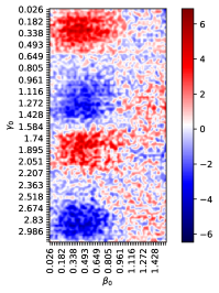
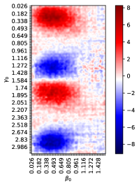
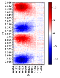
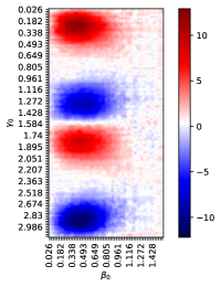
Figure 14: Experimental mean energy landscapes for a $p=1$ QAOA for a 27-qubit instance across 4 IBMQ devices.

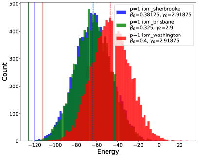
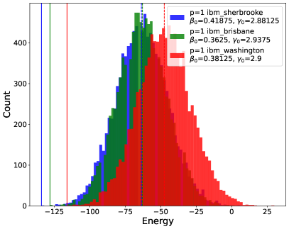
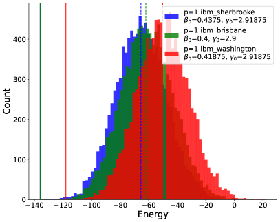
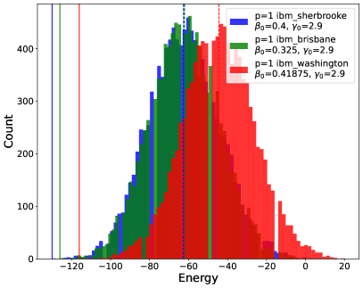
Figure 15: Experimental sample energy distributions for a $p=1$ QAOA for 4 random 127-qubit instances executed across 3 IBMQ devices, for the best device-specific angles found by a focused angle gridsearch. The minimum sample energies and mean energies from these distributions are marked with solid and dashed vertical lines, respectively.

4 Conclusion

We have demonstrated that transfer learning of QAOA angles up to $p=5$ can be successfully applied to large (up to $127$ qubit) systems using training on a single small ($16$ qubit) instance. This provides evidence – in addition to what has been presented in the literature on various other optimization problems – that parameter concentration can be used as an efficient method for computing high-quality (although not necessarily optimal) QAOA angles. We used converged classical MPS simulations with up to a bond dimension of $\chi=2048$ to calculate the noiseless mean expectation values, as well as the smple distributions, of the $127$ qubit QAOA circuits sampling these hardware compatible higher-order Ising model instances using the transfer-learned angles.

We also demonstrated the scaling of whole-chip QAOA on heavy-hex hardware-native spin glass models, with respect to $p$, on several IBM Quantum superconducting qubit processors. This demonstration comprises large circuits that fully evaluate the current performance of these IBM Quantum processors using highly NISQ-friendly and short depth QAOA circuits. We find that the peak of QAOA performance on hardware is at $p=2,3$ on most of the IBM Quantum processors. This result shows the current state of competition between the error inherent in the computation, and the improving approximation ratios from larger $p$ (and good angles learned at higher $p$). These type of sparse short depth circuits are in contrast to dense circuits, such as quantum volume circuits [50, 51], but allow probing of usage of an entire hardware graph. We observed that the relatively simple Pauli X pair digital dynamical decoupling sequences improved the mean QAOA computation on some of the IBM Quantum processors, but not all devices.

While the scale of the number of qubits used in these QAOA simulations far exceeds what can be exactly classically simulated using full state vector simulations, the sparsity of the underlying hardware graph means that simulating the mean expectation value for low QAOA rounds is possible. At high rounds, we expect the classical simulation of such QAOA circuits to also begin to struggle, and an interesting future avenue of study is to determine where this point is. In this work we have used MPS simulations in order to simulate the QAOA circuits up to $p=5$ in order to verify that the parameter transfer procedure was successful, but is unclear how classically simulate-able higher round QAOA is when targeting Ising models defined on heavy-hex graphs. For example, a Hamiltonian dynamics simulation was performed on a $127$ qubit heavy-hex IBM Quantum device [52], the experiments for which were then classically simulated efficiently using a number of different approaches [53, 54, 55, 56, 57, 58, 59, 60, 61]. This suggests that perhaps even high round QAOA circuits for these sparse heavy-hex Ising models may be easy to simulate when the number of qubits is small. It is also of interest to evaluate how well MPS simulations can be applied to these QAOA circuits when the angles are optimal (or nearly-optimal), as opposed to, for example, random QAOA angles. This is a very interesting regime to investigate since it is approaching the boundary of what is classically verifiable - we leave these high $p$ heavy-hex compatible QAOA simulation questions open for future work.

Our findings show that QAOA parameter transfer can be used in order to obtain good angles for QAOA circuits that are very high in qubit count. We expect that these types of transfer learning protocols will be useful in future implementations of QAOA. However, there is an important aspect of this which has not been studied up to this point. This is the case where the QAOA angles computed at a small problem size are so good that they reach an approximation ratio that is effectively $1$ - in other words, the QAOA performance plateaus (as a function of increasing $p$) to optimality. Once this occurs, good angles at higher $p$ can no longer be meaningfully computed for the small problem instance [8, 24, 39], and thus good angles cannot be computed to be used for the larger problem instance. This is related to the question of QAOA scaling (how many $p$ rounds we need in order to obtain good approximation ratios) as a function of increasing $N$. Succinctly, the task of investigating QAOA angle transfer learning for extremely high $p$ should be investigated in future research.

5 Acknowledgments

This work was supported by the U.S. Department of Energy through the Los Alamos National Laboratory. Los Alamos National Laboratory is operated by Triad National Security, LLC, for the National Nuclear Security Administration of U.S. Department of Energy (Contract No. 89233218CNA000001). This research used resources provided by the Los Alamos National Laboratory Institutional Computing Program. We acknowledge the use of IBM Quantum services for this work. The views expressed are those of the authors, and do not reflect the official policy or position of IBM or the IBM Quantum team. The authors thank IBM Quantum Technical Support. The research presented in this article was supported by the Laboratory Directed Research and Development program of Los Alamos National Laboratory under project number 20220656ER and 20230049DR. Research presented in this article was supported by the NNSA’s Advanced Simulation and Computing Beyond Moore’s Law Program at Los Alamos National Laboratory. This research used resources provided by the Darwin testbed at Los Alamos National Laboratory (LANL) which is funded by the Computational Systems and Software Environments subprogram of LANL’s Advanced Simulation and Computing program (NNSA/DOE).

The figures in this article were generated using matplotlib [62, 63], networkx [64], and Qiskit [42] in Python 3. Code and data are available in a public repository .

LA-UR-23-33192

Appendix A Best QAOA angles used for parameter transfer to high qubit heavy-hex circuits

The trained QAOA angles up to $p=5$ on a single $16$ qubit problem instance (with cubic terms) using JuliQAOA [38], which were used for the parameter transfer onto much larger problem instances, are:

• $p_{1}:\beta=[0.38919],\gamma=[6.04302]$

• $p_{2}:\beta=[0.48912,0.27367],\gamma=[6.09758,5.95396]$

• $p_{3}:\beta=[0.50502,0.35713,0.19264],\gamma=[6.14054,6.01729,5.94123]$

• $p_{4}:\beta=[0.54321,0.41806,0.28615,0.16041],\gamma=[6.16242,6.05959,5.98417,5.9299]$

• $p_{5}:\beta=[0.53822,0.44776,0.32923,0.23056,0.12587],\gamma=[6.16555,6.08373,6.01445,5.9616,5.93736]$

Appendix B Compiled Whole-Chip QAOA Circuit drawings

Figure 16 shows the compiled and scheduled $127$ qubit whole chip QAOA circuits ($p=1$) with dynamical decoupling sequences inserted, drawn using Qiskit [42]. The rz gates are virtual gates [65], meaning they have no error rate, and the rz gates are represented as black circular arrow markers. The x gates are represented as vertical green lines, the sx gates are represented as vertical red lines, and the cx gates (e.g. CNOT gates) are represented by vertical blue lines that connect two qubit lines, and the ECR gates are represented by vertical purple lines that connect two qubit lines. The width of the gate instructions represent the time duration of the gates. The state of all qubits are measured at the end of the circuit, represented by dark grey blocks. The ASAP scheduling inserts more pairs of Pauli X gates compared to the ALAP scheduling.

The timeline circuit diagrams proceed as a function of time on the x-axis, and this representation of the circuits shows that the ibm_washington compiled circuits in Figure 16 used more time per circuit to execute a single circuit compared to the ibm_sherbrooke compiled circuits.

Note that the ibm_washington compiled circuits in Figure 16 correspond to QAOA circuits that sample ibm_washington topology native Ising models (see Refs. [25, 26]), which means that there are two missing CNOTs in the hardware graph compared to the ibm_sherbrooke hardware graph.

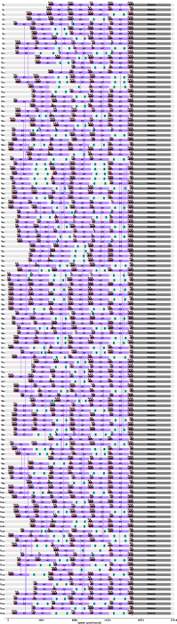
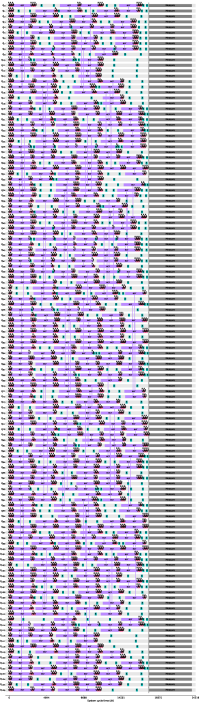
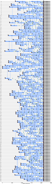
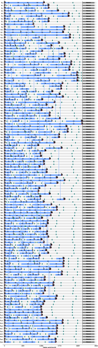
ibm_sherbrooke ALAP ibm_sherbrooke ASAP ibm_washington ALAP ibm_washington ASAP

Figure 16: $p=1$ timeline QAOA circuit for sampling Ising models that contain higher order terms. Compiled to (both left) ibm_sherbrooke with native 2-qubit gate ECR and (both right) ibm_washington with native gate CX.
For both devices, we compile with Pauli X gate pair dynamical decoupling passes inserted and scheduled ALAP (sub left) or ASAP (sub right). Gate times of ECR are more uniform, resulting in a denser gate scheduling, compared to the CX gate times, whose heterogeneity was not considered in the layered circuit design of Figure 2. The ASAP scheduled circuits contain more overall idle qubit time, after a qubit has had at least one gate applied, resulting in more dynamical decoupling sequences being inserted compared to ALAP scheduled circuits.

Appendix C Classical parameter tuning approach: parameter fixing with angle gridsearch

Figure 17 shows that iteratively performing angle gridsearches (using exact classical simulations of the $27$ qubit circuits), and fixing the best angles found at the previous round $p$, unfortunately quickly plateaus to sub-optimal angles, with very little increase from $p=3$ to $p=4$. It may be the case that random local searches around these parameter fixing search spaces yield better angles, but this direct approach of a grid search in additional to parameter fixing of the previous round did not work. Instead, we opted for learning good angles using alternative methods that were able to compute high quality QAOA angles (described in Section 2.3). These angle fixing QAOA numerical simulations shown in Figure 17 were performed using Qiskit [42], where the mean energy for a set of angles was computed using $10,000$ shots. The angle gridsearch was $200$ linearly spaced angles between $(0,\pi)$ (for both axis of the $\beta_{p}$ and $\gamma_{p}$ that were being varied), with the exception of $\beta_{1}$ (for $p=1$) where the linearly spaced gridsearch was cut half to $(0,\frac{\pi}{2})$ (see Section 2.2 for more details). Figure 17 shows the the pure angle fixing approach seems to cause the expectation value of the QAOA landscape to begin to converge - the mechanism behind this could be studied in future work.

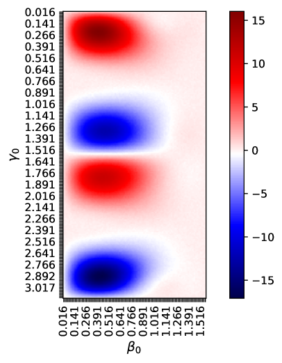
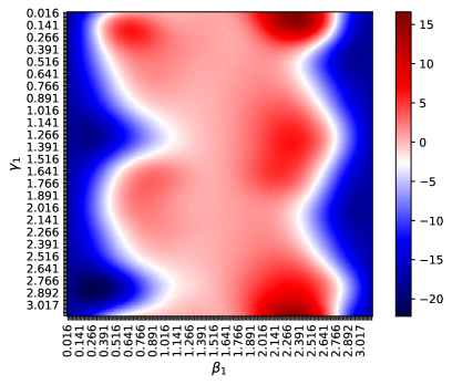
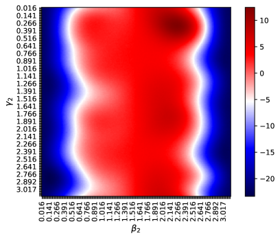
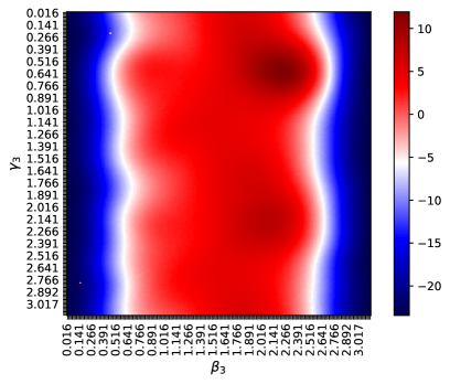
Figure 17: Heatmap showing classical simulation of the mean energy for QAOA angles as $p$ is increased, while fixing good angles found at previous rounds. The fixed angles used based on the parameter fixing gridsearch approach (e.g. the best angles found for each gridsearch, shown in the above heatmaps) is $\beta_{0}=0.422,\gamma_{0}=2.891,\beta_{1}=0.281,\gamma_{1}=2.845,\beta_{2}=0.125,\gamma_{2}=2.813,\beta_{3}=0.047,\gamma_{3}=0.203$ (indexing of $p=1$ is $0$). The problem instance being sampled here is a $27$ qubit random Ising model with cubic terms, defined on the $27$ qubit IBM Quantum processor heavy hex graph. Notably, the mean energy landscapes from $p=2,3,4$ are converging to similar shapes, with very little energy improvement being gained between $p=3$ and $p=4$, showing that this gridsearch and angle fixing method does not work as an angle finding approach, and therefore we utilized the better angle finding methods described in Subsection 2.3.

Appendix D ibm_seattle hardware graph

Figure 18 shows the heavy-hex hardware graph of ibm_seattle, where the red nodes denote de-activated hardware regions that could not be used when executing circuits.

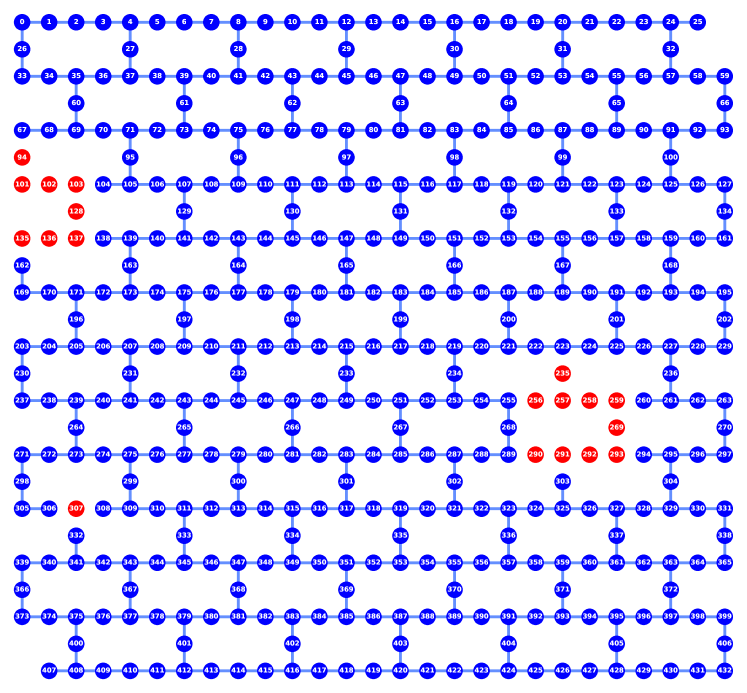
Figure 18: ibm_seattle hardware graph. Red nodes indicate qubits which are hardware de-activated and not available to use at the time of these experiments. The logical hardware graph has $433$ qubits, $19$ of which are de-activated, resulting in a total of $414$ qubits which can be used for executing the short depth QAOA circuits.

Appendix E Optimal Solutions and Minimum QAOA Energy Tables

Table 2 shows the optimal solution energy, along with the minimum energy sampled by the whole-chip QAOA circuits when executed on the IBM Quantum computing hardware, for all $100$ of the $127$ variable higher-order Ising model problem instances. Table 3 (left) shows the same for the $27$ variable problem instances, and Table 3 (right) shows the same for the $16$ variable problem instances. The count of samples that found the minimum energy signals the stability of that measurement. Together, these tables describe the minimum energies sampled from the set of increasing $p$ experiments described in Section 3.2. The count of samples that found the minimum energy is out of $20000\cdot 100\cdot D\cdot 3\cdot 5$ total samples, where $D$ is the number of devices that were used (for $16$ variables $D=1$, for $27$ variables this is $D=6$, and for $127$ variables this is $D=4$).

We observe from Table 2 that both ibm_brisbane and ibm_sherbrooke actually found their best mean values at $p=3$ for a good fraction of the 100 instances (i.e., 36 and 43 instances, respectively); these two backends even found minima at $p=4$ for 9 and 1 of the instances, respectively. Thus, the higher QAOA rounds are close to paying off.

In Table 2, minimum sample energies given for the specific devices are always with respect to the sample distribution for the given $p$ and $\mathit{DD}$ parameters. Lower sample energies are sometimes found at non-optimal (with respect to the mean sample energy) parameters $p$, $\mathit{DD}$. Indeed, the overall QAOA minimum sample energy across all parameters is shown for many instances strictly lower than the given minimum sample energies for the four devices at fixed parameters.

	instance energies		overall QAOA	best ibm_brisbane sample			best ibm_cusco sample			best ibm_nazca sample			best ibm_sherbrooke sample
	ground state	maximum	min sample energy	mean	min	at params	mean	min	at params	mean	min	at params	mean	min	at params
0	-188	202	-150 ($\times$1)	-76.50	-148	p=3, DD=ALAP	-43.30	-120	p=2, DD=ALAP	-61.05	-132	p=2, DD=ALAP	-67.99	-140	p=3, DD=none
1	-196	200	-156 ($\times$1)	-80.18	-154	p=2, DD=ALAP	-48.06	-122	p=2, DD=ALAP	-67.89	-142	p=2, DD=ALAP	-70.13	-148	p=2, DD=none
2	-198	198	-164 ($\times$1)	-79.97	-142	p=2, DD=ALAP	-42.54	-116	p=1, DD=ALAP	-63.28	-130	p=2, DD=ALAP	-68.75	-138	p=2, DD=none
3	-198	196	-156 ($\times$1)	-81.17	-146	p=2, DD=ALAP	-46.52	-114	p=2, DD=ALAP	-64.09	-136	p=2, DD=ALAP	-69.97	-138	p=2, DD=none
4	-196	196	-154 ($\times$1)	-83.95	-154	p=3, DD=ASAP	-48.46	-124	p=1, DD=ALAP	-66.19	-146	p=3, DD=ALAP	-75.87	-144	p=2, DD=none
5	-204	194	-162 ($\times$3)	-86.86	-162	p=2, DD=ALAP	-52.47	-122	p=2, DD=ALAP	-67.48	-138	p=2, DD=ALAP	-73.18	-146	p=3, DD=none
6	-182	196	-150 ($\times$1)	-80.15	-144	p=2, DD=ALAP	-45.05	-118	p=2, DD=ALAP	-68.19	-134	p=2, DD=ALAP	-72.39	-136	p=3, DD=none
7	-204	192	-158 ($\times$2)	-84.04	-152	p=2, DD=ALAP	-48.90	-124	p=2, DD=ALAP	-64.89	-142	p=3, DD=ALAP	-73.45	-142	p=2, DD=none
8	-192	194	-150 ($\times$1)	-81.69	-144	p=3, DD=ALAP	-43.72	-116	p=1, DD=ALAP	-66.76	-130	p=2, DD=ALAP	-68.89	-138	p=2, DD=none
9	-200	202	-154 ($\times$2)	-86.35	-152	p=2, DD=ALAP	-48.51	-122	p=1, DD=ALAP	-67.43	-136	p=3, DD=ALAP	-76.69	-146	p=2, DD=none
10	-198	192	-154 ($\times$2)	-82.44	-146	p=2, DD=ALAP	-46.11	-110	p=2, DD=ALAP	-67.38	-140	p=2, DD=ALAP	-73.74	-142	p=2, DD=none
11	-206	196	-160 ($\times$3)	-84.46	-156	p=2, DD=ALAP	-47.03	-122	p=2, DD=ALAP	-68.22	-144	p=3, DD=ALAP	-70.07	-138	p=2, DD=none
12	-198	198	-158 ($\times$1)	-80.13	-158	p=2, DD=ALAP	-45.32	-114	p=1, DD=ALAP	-63.81	-130	p=3, DD=ASAP	-71.95	-140	p=2, DD=none
13	-202	200	-158 ($\times$1)	-79.69	-154	p=2, DD=ALAP	-48.52	-118	p=2, DD=ALAP	-64.90	-140	p=3, DD=ALAP	-70.69	-138	p=3, DD=none
14	-182	198	-154 ($\times$1)	-79.73	-154	p=3, DD=ALAP	-47.68	-116	p=2, DD=ALAP	-64.79	-136	p=3, DD=ALAP	-69.53	-132	p=2, DD=none
15	-200	190	-160 ($\times$1)	-83.22	-160	p=3, DD=ALAP	-51.02	-120	p=2, DD=ALAP	-67.50	-134	p=2, DD=ASAP	-70.34	-140	p=2, DD=none
16	-198	198	-160 ($\times$2)	-80.98	-160	p=3, DD=ALAP	-48.03	-122	p=2, DD=ALAP	-67.19	-136	p=3, DD=ALAP	-72.10	-142	p=2, DD=none
17	-188	182	-152 ($\times$3)	-78.65	-144	p=3, DD=ALAP	-47.79	-118	p=2, DD=ALAP	-64.56	-138	p=2, DD=ALAP	-69.61	-134	p=3, DD=none
18	-202	190	-160 ($\times$2)	-81.83	-150	p=2, DD=ALAP	-45.69	-126	p=2, DD=ALAP	-64.96	-144	p=3, DD=ALAP	-73.13	-142	p=2, DD=none
19	-200	196	-162 ($\times$2)	-83.27	-158	p=2, DD=ALAP	-46.21	-114	p=1, DD=ALAP	-61.74	-130	p=2, DD=ASAP	-70.73	-142	p=2, DD=none
20	-204	186	-160 ($\times$1)	-82.11	-156	p=3, DD=ALAP	-46.46	-118	p=2, DD=ALAP	-67.00	-140	p=3, DD=ALAP	-73.99	-148	p=2, DD=none
21	-194	200	-160 ($\times$1)	-80.87	-142	p=3, DD=ALAP	-45.12	-118	p=2, DD=ALAP	-65.24	-138	p=3, DD=ALAP	-70.59	-136	p=2, DD=none
22	-216	196	-166 ($\times$1)	-85.40	-156	p=3, DD=ALAP	-44.32	-110	p=2, DD=ALAP	-68.27	-162	p=2, DD=ALAP	-74.13	-152	p=3, DD=none
23	-198	204	-158 ($\times$1)	-81.29	-152	p=4, DD=ALAP	-44.88	-114	p=2, DD=ALAP	-64.74	-136	p=2, DD=ASAP	-72.99	-146	p=3, DD=none
24	-202	194	-158 ($\times$1)	-83.97	-158	p=2, DD=ALAP	-49.08	-118	p=2, DD=ALAP	-67.88	-144	p=3, DD=ALAP	-74.36	-144	p=2, DD=none
25	-192	190	-156 ($\times$1)	-80.85	-156	p=3, DD=ALAP	-47.11	-114	p=2, DD=ALAP	-63.67	-138	p=2, DD=ALAP	-71.20	-136	p=3, DD=none
26	-198	194	-158 ($\times$2)	-82.79	-158	p=2, DD=ALAP	-47.85	-116	p=2, DD=ALAP	-69.55	-148	p=2, DD=ASAP	-74.40	-148	p=3, DD=none
27	-198	208	-150 ($\times$1)	-78.85	-148	p=3, DD=ASAP	-49.53	-120	p=2, DD=ALAP	-64.84	-138	p=2, DD=ALAP	-70.88	-136	p=2, DD=none
28	-194	190	-152 ($\times$1)	-79.58	-146	p=2, DD=ALAP	-47.34	-114	p=1, DD=ALAP	-64.00	-138	p=2, DD=ALAP	-71.53	-144	p=3, DD=none
29	-196	196	-152 ($\times$1)	-80.95	-144	p=2, DD=ALAP	-46.39	-116	p=1, DD=ALAP	-65.08	-132	p=2, DD=ALAP	-72.81	-140	p=2, DD=none
30	-196	200	-160 ($\times$1)	-79.33	-150	p=2, DD=ALAP	-47.08	-114	p=1, DD=ALAP	-62.90	-132	p=2, DD=ASAP	-70.87	-138	p=2, DD=none
31	-200	196	-154 ($\times$1)	-82.09	-150	p=2, DD=ALAP	-48.07	-124	p=2, DD=ALAP	-64.29	-128	p=2, DD=ALAP	-74.18	-154	p=2, DD=none
32	-194	182	-152 ($\times$2)	-80.87	-150	p=2, DD=ALAP	-50.59	-118	p=2, DD=ALAP	-64.37	-134	p=3, DD=ALAP	-68.28	-140	p=3, DD=none
33	-206	192	-170 ($\times$1)	-81.50	-152	p=2, DD=ALAP	-46.62	-130	p=2, DD=ALAP	-67.57	-150	p=3, DD=ALAP	-75.39	-146	p=3, DD=none
34	-190	208	-148 ($\times$1)	-79.68	-148	p=3, DD=ALAP	-44.12	-116	p=2, DD=ALAP	-66.63	-130	p=3, DD=ALAP	-71.01	-130	p=2, DD=none
35	-206	202	-164 ($\times$1)	-84.09	-154	p=4, DD=ALAP	-45.83	-110	p=2, DD=ALAP	-64.05	-146	p=2, DD=ALAP	-71.38	-140	p=2, DD=none
36	-202	196	-156 ($\times$6)	-86.80	-156	p=2, DD=ALAP	-49.90	-132	p=2, DD=ALAP	-71.04	-140	p=3, DD=ASAP	-75.27	-140	p=2, DD=none
37	-190	204	-154 ($\times$1)	-78.56	-144	p=3, DD=ALAP	-45.76	-122	p=2, DD=ALAP	-63.80	-132	p=3, DD=ALAP	-70.88	-140	p=2, DD=none
38	-184	192	-150 ($\times$2)	-78.26	-150	p=2, DD=ALAP	-43.86	-114	p=2, DD=ALAP	-61.96	-130	p=2, DD=ALAP	-71.17	-138	p=3, DD=none
39	-206	190	-156 ($\times$4)	-82.67	-156	p=2, DD=ALAP	-44.77	-116	p=2, DD=ALAP	-65.37	-134	p=3, DD=ALAP	-72.53	-152	p=4, DD=none
40	-196	204	-158 ($\times$1)	-78.58	-158	p=3, DD=ALAP	-45.80	-120	p=1, DD=ALAP	-62.23	-130	p=2, DD=ASAP	-70.65	-138	p=2, DD=none
41	-192	190	-150 ($\times$1)	-77.36	-144	p=3, DD=ALAP	-46.95	-124	p=1, DD=ALAP	-61.01	-132	p=2, DD=ASAP	-67.56	-132	p=2, DD=none
42	-218	202	-164 ($\times$1)	-85.96	-154	p=2, DD=ALAP	-51.18	-128	p=2, DD=ALAP	-64.57	-136	p=2, DD=ASAP	-74.02	-146	p=2, DD=none
43	-198	198	-156 ($\times$1)	-83.41	-152	p=3, DD=ALAP	-48.03	-128	p=2, DD=ALAP	-64.65	-132	p=2, DD=ASAP	-69.73	-140	p=2, DD=none
44	-206	190	-166 ($\times$2)	-86.63	-156	p=4, DD=ALAP	-48.53	-120	p=1, DD=ALAP	-69.93	-140	p=2, DD=ALAP	-71.51	-142	p=3, DD=none
45	-212	190	-166 ($\times$1)	-84.47	-154	p=3, DD=ALAP	-46.22	-128	p=1, DD=ALAP	-66.93	-136	p=2, DD=ALAP	-70.21	-146	p=2, DD=none
46	-202	198	-168 ($\times$1)	-83.90	-158	p=4, DD=ALAP	-45.60	-120	p=2, DD=ALAP	-66.84	-146	p=2, DD=ALAP	-72.27	-142	p=2, DD=none
47	-192	190	-156 ($\times$1)	-82.92	-144	p=2, DD=ALAP	-46.08	-118	p=2, DD=ALAP	-68.31	-132	p=3, DD=ALAP	-67.50	-136	p=3, DD=none
48	-188	186	-154 ($\times$1)	-80.78	-154	p=4, DD=ALAP	-46.01	-124	p=1, DD=ALAP	-64.40	-124	p=2, DD=ALAP	-71.25	-138	p=3, DD=none
49	-210	186	-176 ($\times$1)	-86.88	-168	p=3, DD=ALAP	-48.88	-126	p=2, DD=ALAP	-68.97	-146	p=2, DD=ALAP	-70.59	-142	p=2, DD=none
50	-186	202	-150 ($\times$2)	-82.98	-144	p=2, DD=ALAP	-48.21	-124	p=2, DD=ALAP	-64.00	-130	p=2, DD=ASAP	-69.22	-134	p=2, DD=none
51	-192	192	-150 ($\times$1)	-82.73	-144	p=2, DD=ALAP	-48.29	-124	p=2, DD=ALAP	-61.66	-130	p=2, DD=ALAP	-72.11	-142	p=2, DD=none
52	-202	194	-158 ($\times$2)	-82.34	-158	p=4, DD=ASAP	-48.04	-116	p=2, DD=ALAP	-60.74	-134	p=2, DD=ASAP	-68.28	-144	p=3, DD=none
53	-194	214	-154 ($\times$1)	-81.78	-144	p=2, DD=ALAP	-47.87	-110	p=1, DD=ALAP	-67.16	-136	p=3, DD=ALAP	-71.14	-132	p=3, DD=none
54	-208	200	-158 ($\times$1)	-81.03	-150	p=2, DD=ALAP	-50.15	-114	p=2, DD=ALAP	-66.23	-134	p=2, DD=ALAP	-71.47	-142	p=2, DD=none
55	-194	196	-160 ($\times$1)	-85.15	-154	p=3, DD=ALAP	-48.12	-112	p=2, DD=ALAP	-66.11	-136	p=2, DD=ASAP	-75.02	-140	p=2, DD=none
56	-200	188	-156 ($\times$1)	-84.11	-154	p=3, DD=ALAP	-48.74	-124	p=2, DD=ALAP	-65.45	-134	p=2, DD=ALAP	-72.34	-138	p=3, DD=none
57	-192	188	-156 ($\times$1)	-79.15	-142	p=3, DD=ALAP	-41.94	-108	p=1, DD=ALAP	-61.65	-140	p=2, DD=ALAP	-67.74	-132	p=2, DD=none
58	-202	202	-154 ($\times$3)	-78.48	-152	p=2, DD=ALAP	-45.46	-116	p=2, DD=ALAP	-63.29	-130	p=2, DD=ALAP	-70.29	-146	p=2, DD=none
59	-212	182	-166 ($\times$2)	-88.49	-158	p=2, DD=ALAP	-52.16	-130	p=2, DD=ALAP	-66.81	-154	p=2, DD=ALAP	-72.04	-160	p=3, DD=none
60	-208	180	-174 ($\times$1)	-86.19	-154	p=3, DD=ALAP	-44.94	-122	p=1, DD=ALAP	-65.20	-138	p=2, DD=ALAP	-69.82	-150	p=2, DD=none
61	-194	208	-150 ($\times$1)	-81.90	-142	p=2, DD=ALAP	-44.48	-110	p=1, DD=ALAP	-64.20	-130	p=2, DD=ALAP	-71.58	-132	p=2, DD=none
62	-202	196	-152 ($\times$2)	-80.37	-146	p=2, DD=ALAP	-44.43	-116	p=2, DD=ALAP	-65.08	-134	p=2, DD=ALAP	-67.74	-140	p=3, DD=none
63	-208	192	-166 ($\times$1)	-84.85	-166	p=3, DD=ALAP	-48.54	-118	p=2, DD=ALAP	-66.42	-152	p=2, DD=ALAP	-73.29	-154	p=2, DD=none
64	-200	202	-158 ($\times$1)	-82.51	-148	p=2, DD=ALAP	-49.25	-118	p=2, DD=ALAP	-66.91	-140	p=2, DD=ALAP	-73.56	-142	p=2, DD=none
65	-200	206	-152 ($\times$4)	-79.76	-140	p=2, DD=ALAP	-47.29	-116	p=2, DD=ALAP	-67.56	-134	p=2, DD=ALAP	-72.74	-140	p=3, DD=none
66	-204	188	-158 ($\times$2)	-83.04	-154	p=2, DD=ALAP	-45.51	-114	p=2, DD=ALAP	-65.10	-150	p=3, DD=ALAP	-72.54	-144	p=3, DD=none
67	-196	202	-158 ($\times$1)	-83.09	-154	p=3, DD=ALAP	-44.72	-114	p=2, DD=ALAP	-65.67	-132	p=2, DD=ALAP	-72.22	-144	p=3, DD=none
68	-204	184	-162 ($\times$1)	-84.08	-162	p=3, DD=ALAP	-43.25	-116	p=1, DD=ALAP	-68.52	-144	p=3, DD=ALAP	-71.11	-148	p=3, DD=none
69	-186	196	-152 ($\times$1)	-80.54	-148	p=2, DD=ALAP	-43.00	-124	p=2, DD=ALAP	-62.29	-132	p=2, DD=ALAP	-68.31	-132	p=3, DD=none
70	-194	196	-152 ($\times$3)	-79.24	-142	p=2, DD=ALAP	-46.98	-110	p=2, DD=ALAP	-64.09	-130	p=2, DD=ALAP	-72.93	-152	p=3, DD=none
71	-192	184	-156 ($\times$1)	-80.06	-150	p=4, DD=ALAP	-45.94	-112	p=2, DD=ALAP	-66.14	-142	p=3, DD=ALAP	-69.73	-140	p=2, DD=none
72	-190	190	-150 ($\times$1)	-83.54	-146	p=2, DD=ALAP	-49.92	-126	p=1, DD=ALAP	-65.14	-136	p=2, DD=ALAP	-71.05	-134	p=3, DD=none
73	-194	194	-160 ($\times$1)	-82.96	-154	p=3, DD=ALAP	-46.31	-116	p=2, DD=ALAP	-65.35	-136	p=2, DD=ALAP	-73.13	-136	p=2, DD=none
74	-188	218	-146 ($\times$1)	-79.39	-140	p=3, DD=ALAP	-49.73	-118	p=2, DD=ALAP	-66.34	-132	p=2, DD=ALAP	-68.28	-132	p=3, DD=none
75	-202	196	-162 ($\times$1)	-82.93	-158	p=3, DD=ALAP	-50.31	-118	p=2, DD=ALAP	-68.84	-146	p=2, DD=ALAP	-71.15	-146	p=2, DD=none
76	-186	200	-144 ($\times$1)	-79.21	-140	p=2, DD=ALAP	-46.79	-114	p=2, DD=ALAP	-67.52	-138	p=2, DD=ALAP	-74.88	-136	p=3, DD=none
77	-204	196	-152 ($\times$1)	-83.49	-148	p=2, DD=ALAP	-47.08	-130	p=1, DD=ALAP	-66.10	-138	p=3, DD=ASAP	-71.61	-140	p=3, DD=none
78	-198	196	-152 ($\times$1)	-82.51	-148	p=3, DD=ALAP	-46.89	-112	p=2, DD=ALAP	-63.64	-134	p=2, DD=ASAP	-72.54	-144	p=2, DD=none
79	-206	192	-156 ($\times$2)	-80.16	-156	p=2, DD=ASAP	-45.54	-114	p=1, DD=ALAP	-66.14	-136	p=2, DD=ALAP	-68.94	-138	p=3, DD=none
80	-198	184	-162 ($\times$1)	-85.67	-156	p=4, DD=ALAP	-47.32	-112	p=2, DD=ALAP	-65.56	-136	p=3, DD=ALAP	-73.44	-142	p=3, DD=none
81	-196	196	-156 ($\times$1)	-82.98	-152	p=2, DD=ALAP	-48.05	-116	p=2, DD=ALAP	-63.20	-130	p=2, DD=ALAP	-73.60	-146	p=3, DD=none
82	-192	200	-152 ($\times$2)	-78.50	-152	p=2, DD=ALAP	-44.80	-116	p=2, DD=ALAP	-64.75	-128	p=2, DD=ALAP	-69.70	-130	p=3, DD=none
83	-192	194	-154 ($\times$1)	-85.96	-152	p=2, DD=ALAP	-47.70	-118	p=2, DD=ALAP	-67.02	-146	p=3, DD=ALAP	-77.91	-152	p=2, DD=none
84	-206	186	-166 ($\times$1)	-88.27	-166	p=3, DD=ASAP	-51.70	-122	p=2, DD=ALAP	-69.01	-150	p=3, DD=ALAP	-77.46	-142	p=2, DD=none
85	-196	200	-154 ($\times$2)	-83.82	-154	p=3, DD=ALAP	-47.38	-118	p=2, DD=ALAP	-64.76	-130	p=2, DD=ALAP	-71.25	-144	p=3, DD=none
86	-200	206	-158 ($\times$2)	-80.00	-158	p=4, DD=ALAP	-44.95	-122	p=1, DD=ALAP	-63.87	-140	p=2, DD=ALAP	-69.19	-134	p=3, DD=none
87	-204	178	-160 ($\times$1)	-86.58	-158	p=2, DD=ALAP	-49.31	-120	p=2, DD=ALAP	-70.03	-142	p=2, DD=ALAP	-77.74	-150	p=2, DD=none
88	-196	194	-154 ($\times$1)	-79.74	-146	p=2, DD=ALAP	-45.30	-112	p=2, DD=ALAP	-62.02	-152	p=3, DD=ASAP	-73.22	-138	p=3, DD=none
89	-192	204	-150 ($\times$1)	-78.42	-146	p=2, DD=ALAP	-47.24	-116	p=2, DD=ALAP	-61.94	-122	p=3, DD=ALAP	-70.08	-134	p=3, DD=none
90	-208	204	-162 ($\times$2)	-84.22	-156	p=2, DD=ALAP	-46.32	-120	p=2, DD=ALAP	-64.64	-136	p=2, DD=ALAP	-68.90	-142	p=3, DD=none
91	-198	194	-156 ($\times$1)	-81.15	-156	p=4, DD=ALAP	-41.78	-122	p=2, DD=ALAP	-63.84	-130	p=2, DD=ALAP	-66.13	-148	p=2, DD=none
92	-206	192	-162 ($\times$1)	-80.94	-158	p=3, DD=ALAP	-44.02	-110	p=1, DD=ALAP	-63.60	-138	p=2, DD=ASAP	-68.01	-156	p=3, DD=none
93	-188	192	-150 ($\times$1)	-78.66	-138	p=2, DD=ALAP	-45.06	-116	p=2, DD=ALAP	-62.83	-126	p=2, DD=ALAP	-70.88	-144	p=2, DD=none
94	-200	194	-156 ($\times$1)	-83.31	-154	p=3, DD=ALAP	-44.73	-116	p=2, DD=ALAP	-64.58	-132	p=2, DD=ALAP	-73.90	-138	p=2, DD=none
95	-198	184	-156 ($\times$1)	-81.58	-150	p=2, DD=ALAP	-46.13	-114	p=2, DD=ALAP	-65.60	-142	p=2, DD=ALAP	-70.02	-144	p=3, DD=none
96	-194	202	-150 ($\times$2)	-80.98	-150	p=3, DD=ALAP	-44.02	-118	p=2, DD=ALAP	-65.37	-136	p=2, DD=ASAP	-71.41	-134	p=3, DD=none
97	-198	192	-162 ($\times$1)	-82.55	-150	p=2, DD=ALAP	-45.90	-114	p=2, DD=ALAP	-62.76	-132	p=3, DD=ALAP	-70.73	-134	p=2, DD=none
98	-202	196	-154 ($\times$4)	-83.37	-154	p=3, DD=ALAP	-46.38	-116	p=1, DD=ALAP	-68.35	-146	p=2, DD=ALAP	-71.34	-146	p=3, DD=none
99	-188	192	-150 ($\times$1)	-82.46	-146	p=3, DD=ALAP	-43.76	-108	p=2, DD=ALAP	-64.69	-132	p=2, DD=ALAP	-70.31	-150	p=2, DD=none

Table 2: Summary of the most successful QAOA runs for all 100 random 127-qubit instances on 4 IBMQ devices: We give the overall QAOA minimum sample energy across $20,000$ shots each on all $4$ devices, for each layer number $1\leq p\leq 5$, and for each of the $3$ dynamical decoupling schemes $\mathit{DD}$, counting multiplicities. For each device, we give the parameters $p$ and $\mathit{DD}$ that achieve the best sample mean and also show the sample minimum for these.

$27$-qubit	instance energies		overall	QAOA
instance	ground state	maximum	min sample	energy
0	-42	32	-42 ($\times$	466)
1	-36	40	-36 ($\times$	946)
2	-38	40	-38 ($\times$	108)
3	-36	42	-36 ($\times$	146)
4	-36	44	-36 ($\times$	230)
5	-42	38	-42 ($\times$	342)
6	-40	38	-40 ($\times$	282)
7	-42	32	-42 ($\times$	150)
8	-42	38	-42 ($\times$	234)
9	-44	44	-44 ($\times$	138)
10	-42	38	-42 ($\times$	285)
11	-40	40	-40 ($\times$	225)
12	-38	42	-38 ($\times$	164)
13	-36	38	-36 ($\times$	540)
14	-40	34	-40 ($\times$	143)
15	-34	34	-34 ($\times$	3602)
16	-38	38	-38 ($\times$	221)
17	-40	34	-40 ($\times$	170)
18	-42	36	-42 ($\times$	303)
19	-36	36	-36 ($\times$	693)
20	-34	42	-34 ($\times$	130)
21	-36	34	-36 ($\times$	321)
22	-36	40	-36 ($\times$	336)
23	-36	36	-36 ($\times$	2315)
24	-34	40	-34 ($\times$	817)
25	-38	38	-38 ($\times$	455)
26	-38	38	-38 ($\times$	512)
27	-46	38	-46 ($\times$	65)
28	-32	36	-32 ($\times$	636)
29	-34	40	-34 ($\times$	738)
30	-36	50	-36 ($\times$	64)
31	-40	34	-40 ($\times$	592)
32	-44	38	-44 ($\times$	98)
33	-36	34	-36 ($\times$	50)
34	-32	38	-32 ($\times$	1015)
35	-40	34	-40 ($\times$	2213)
36	-38	42	-38 ($\times$	444)
37	-32	36	-32 ($\times$	2162)
38	-34	40	-34 ($\times$	247)
39	-38	32	-38 ($\times$	747)
40	-36	44	-36 ($\times$	198)
41	-38	40	-38 ($\times$	291)
42	-38	40	-38 ($\times$	445)
43	-38	38	-38 ($\times$	2899)
44	-36	38	-36 ($\times$	1023)
45	-42	44	-42 ($\times$	348)
46	-40	44	-40 ($\times$	54)
47	-36	42	-36 ($\times$	549)
48	-42	38	-42 ($\times$	337)
49	-44	40	-44 ($\times$	243)
50	-38	42	-38 ($\times$	1175)
51	-38	38	-38 ($\times$	103)
52	-34	42	-34 ($\times$	521)
53	-40	46	-40 ($\times$	286)
54	-38	36	-38 ($\times$	234)
55	-40	46	-40 ($\times$	88)
56	-42	34	-42 ($\times$	647)
57	-40	40	-40 ($\times$	311)
58	-38	38	-38 ($\times$	487)
59	-40	40	-40 ($\times$	307)
60	-34	40	-34 ($\times$	967)
61	-44	38	-44 ($\times$	250)
62	-36	34	-36 ($\times$	1049)
63	-38	40	-38 ($\times$	131)
64	-36	36	-36 ($\times$	1999)
65	-38	36	-38 ($\times$	1233)
66	-42	32	-42 ($\times$	1404)
67	-44	40	-44 ($\times$	510)
68	-42	34	-42 ($\times$	221)
69	-36	36	-36 ($\times$	1019)
70	-40	40	-40 ($\times$	559)
71	-40	40	-40 ($\times$	899)
72	-42	34	-42 ($\times$	555)
73	-44	38	-44 ($\times$	873)
74	-36	40	-36 ($\times$	942)
75	-40	44	-40 ($\times$	20)
76	-38	40	-38 ($\times$	315)
77	-40	32	-40 ($\times$	395)
78	-38	40	-38 ($\times$	170)
79	-40	40	-40 ($\times$	1190)
80	-36	36	-36 ($\times$	949)
81	-40	38	-40 ($\times$	1396)
82	-36	40	-36 ($\times$	1052)
83	-42	48	-42 ($\times$	96)
84	-42	36	-42 ($\times$	138)
85	-40	38	-40 ($\times$	600)
86	-36	38	-36 ($\times$	1645)
87	-40	38	-40 ($\times$	241)
88	-36	40	-36 ($\times$	2150)
89	-36	36	-36 ($\times$	430)
90	-34	40	-34 ($\times$	361)
91	-38	38	-38 ($\times$	406)
92	-34	40	-34 ($\times$	2145)
93	-46	42	-46 ($\times$	73)
94	-40	38	-40 ($\times$	116)
95	-38	38	-38 ($\times$	605)
96	-36	44	-36 ($\times$	765)
97	-36	34	-36 ($\times$	827)
98	-40	40	-40 ($\times$	399)
99	-38	34	-38 ($\times$	1983)

$16$-qubit	instance energies		overall	QAOA
instance	ground state	maximum	min sample	energy
0	-22	22	-22 ($\times$	493)
1	-20	24	-20 ($\times$	3293)
2	-20	18	-20 ($\times$	4112)
3	-26	26	-26 ($\times$	529)
4	-20	20	-20 ($\times$	1804)
5	-24	18	-24 ($\times$	836)
6	-20	24	-20 ($\times$	3213)
7	-22	22	-22 ($\times$	3368)
8	-24	24	-24 ($\times$	668)
9	-24	24	-24 ($\times$	1071)
10	-24	18	-24 ($\times$	1671)
11	-22	18	-22 ($\times$	4183)
12	-22	20	-22 ($\times$	8093)
13	-22	24	-22 ($\times$	3373)
14	-20	20	-20 ($\times$	6119)
15	-24	20	-24 ($\times$	3854)
16	-24	24	-24 ($\times$	265)
17	-20	20	-20 ($\times$	1865)
18	-22	26	-22 ($\times$	3470)
19	-22	26	-22 ($\times$	443)
20	-24	20	-24 ($\times$	4980)
21	-22	18	-22 ($\times$	4526)
22	-20	26	-20 ($\times$	2338)
23	-24	22	-24 ($\times$	3674)
24	-20	24	-20 ($\times$	924)
25	-24	22	-24 ($\times$	3166)
26	-20	24	-20 ($\times$	6678)
27	-22	26	-22 ($\times$	399)
28	-24	20	-24 ($\times$	3079)
29	-20	24	-20 ($\times$	6886)
30	-20	24	-20 ($\times$	647)
31	-24	20	-24 ($\times$	2072)
32	-26	20	-26 ($\times$	1106)
33	-20	22	-20 ($\times$	2860)
34	-20	20	-20 ($\times$	6171)
35	-24	20	-24 ($\times$	3420)
36	-18	24	-18 ($\times$	12616)
37	-20	20	-20 ($\times$	4825)
38	-24	22	-24 ($\times$	1269)
39	-22	20	-22 ($\times$	2189)
40	-24	24	-24 ($\times$	2063)
41	-24	22	-24 ($\times$	1345)
42	-20	24	-20 ($\times$	2080)
43	-22	26	-22 ($\times$	1407)
44	-20	26	-20 ($\times$	1615)
45	-24	20	-24 ($\times$	2165)
46	-22	24	-22 ($\times$	4005)
47	-26	18	-26 ($\times$	1501)
48	-20	28	-20 ($\times$	1276)
49	-24	20	-24 ($\times$	2858)
50	-22	26	-22 ($\times$	1069)
51	-20	20	-20 ($\times$	1665)
52	-26	22	-26 ($\times$	1703)
53	-24	26	-24 ($\times$	316)
54	-26	22	-26 ($\times$	665)
55	-28	20	-28 ($\times$	2560)
56	-22	22	-22 ($\times$	4350)
57	-26	22	-26 ($\times$	945)
58	-22	24	-22 ($\times$	2609)
59	-28	20	-28 ($\times$	1511)
60	-26	20	-26 ($\times$	509)
61	-24	20	-24 ($\times$	675)
62	-22	20	-22 ($\times$	1399)
63	-20	24	-20 ($\times$	2315)
64	-26	22	-26 ($\times$	904)
65	-18	20	-18 ($\times$	10580)
66	-24	26	-24 ($\times$	2729)
67	-24	24	-24 ($\times$	6442)
68	-20	18	-20 ($\times$	2098)
69	-20	24	-20 ($\times$	725)
70	-24	22	-24 ($\times$	1003)
71	-24	24	-24 ($\times$	2151)
72	-20	24	-20 ($\times$	990)
73	-20	22	-20 ($\times$	2952)
74	-26	22	-26 ($\times$	3743)
75	-20	26	-20 ($\times$	2847)
76	-20	20	-20 ($\times$	5321)
77	-26	22	-26 ($\times$	1169)
78	-22	22	-22 ($\times$	2885)
79	-20	22	-20 ($\times$	3244)
80	-24	22	-24 ($\times$	761)
81	-18	26	-18 ($\times$	6474)
82	-24	20	-24 ($\times$	1523)
83	-26	18	-26 ($\times$	812)
84	-20	24	-20 ($\times$	1692)
85	-26	24	-26 ($\times$	634)
86	-20	22	-20 ($\times$	6212)
87	-22	22	-22 ($\times$	3950)
88	-22	28	-22 ($\times$	334)
89	-24	20	-24 ($\times$	2507)
90	-18	22	-18 ($\times$	8225)
91	-26	20	-26 ($\times$	1526)
92	-30	26	-30 ($\times$	825)
93	-20	18	-20 ($\times$	3139)
94	-22	22	-22 ($\times$	1305)
95	-20	26	-20 ($\times$	656)
96	-24	22	-24 ($\times$	3101)
97	-22	20	-22 ($\times$	1430)
98	-20	24	-20 ($\times$	6131)
99	-20	20	-20 ($\times$	4196)

Table 3: Summary of the hardware runs of all 100 random $27$-qubit instances and all 100 random $16$-qubit instances: (left) $27$-qubit instances: We give the overall QAOA minimum sample energy across 20,000 shots each run on all 6 IBMQ devices, for all $1\leq p\leq 5$, and for all 3 dynamical decoupling schemes, also counting multiple appearances. (right) $16$-qubit instances: We give the same QAOA minimum sample data, with instances run on ibm_guadalupe. For each of the 200 instances, the groundstate energy was found multiple times, though not necessarily in each of the experiments (e.g., for $27$-qubit instance $75$, where the groundstate was found 20 times across the $90$ experiments).

References

- [1] Stuart Hadfield et al. “From the Quantum Approximate Optimization Algorithm to a Quantum Alternating Operator Ansatz” In Algorithms 12.2, 2019, pp. 34 DOI: 10.3390/a12020034
- [2] Edward Farhi, Jeffrey Goldstone and Sam Gutmann “A Quantum Approximate Optimization Algorithm” In arXiv preprint, 2014 DOI: 10.48550/arxiv.1411.4028
- [3] Edward Farhi, Jeffrey Goldstone and Sam Gutmann “A Quantum Approximate Optimization Algorithm Applied to a Bounded Occurrence Constraint Problem” In arXiv preprint, 2014 DOI: 10.48550/arXiv.1412.6062
- [4] Lennart Bittel and Martin Kliesch “Training Variational Quantum Algorithms Is NP-Hard” In Physical Review Letters 127.12, 2021, pp. 120502 DOI: 10.1103/physrevlett.127.120502
- [5] Samson Wang et al. “Noise-induced barren plateaus in variational quantum algorithms” In Nature Communications 12, 2021, pp. 6961 DOI: 10.1038/s41467-021-27045-6
- [6] John Preskill “Quantum Computing in the NISQ era and beyond” In Quantum 2, 2018, pp. 79 DOI: 10.22331/q-2018-08-06-79
- [7] Ruslan Shaydulin and Marco Pistoia “QAOA with ” In IEEE International Conference on Quantum Computing & Engineering QCE’23, 2023, pp. 1074–1077 DOI: 10.1109/QCE57702.2023.00121
- [8] Elijah Pelofske, Andreas Bärtschi, John Golden and Stephan Eidenbenz “High-Round QAOA for MAX k-SAT on Trapped Ion NISQ Devices” In IEEE International Conference on Quantum Computing & Engineering QCE’23, 2023, pp. 506–517 DOI: 10.1109/QCE57702.2023.00064
- [9] Matthew P. Harrigan et al. “Quantum approximate optimization of non-planar graph problems on a planar superconducting processor” In Nature Physics 17.3, 2021, pp. 332–336 DOI: 10.1038/s41567-020-01105-y
- [10] Stefan H. Sack and Daniel J. Egger “Large-scale quantum approximate optimization on non-planar graphs with machine learning noise mitigation” In arXiv preprint, 2023 DOI: 10.48550/arXiv.2307.14427
- [11] Johannes Weidenfeller et al. “Scaling of the quantum approximate optimization algorithm on superconducting qubit based hardware” In Quantum 6, 2022, pp. 870 DOI: 10.22331/q-2022-12-07-870
- [12] Ruslan Shaydulin et al. “Evidence of Scaling Advantage for the Quantum Approximate Optimization Algorithm on a Classically Intractable Problem” In arXiv preprint, 2023 DOI: 10.48550/arXiv.2308.02342
- [13] Phillip C. Lotshaw et al. “Scaling quantum approximate optimization on near-term hardware” In Scientific Reports 12.1, 2022, pp. 12388 DOI: 10.1038/s41598-022-14767-w
- [14] Zichang He et al. “Alignment between initial state and mixer improves QAOA performance for constrained optimization” In npj Quantum Information 9.1, 2023, pp. 121 DOI: 10.1038/s41534-023-00787-5
- [15] Andreas Bärtschi and Stephan Eidenbenz “Grover Mixers for QAOA: Shifting Complexity from Mixer Design to State Preparation” In IEEE International Conference on Quantum Computing & Engineering QCE’20, 2020, pp. 72–82 DOI: 10.1109/QCE49297.2020.00020
- [16] John Golden, Andreas Bärtschi, Daniel O’Malley and Stephan Eidenbenz “Threshold-Based Quantum Optimization” In IEEE International Conference on Quantum Computing & Engineering QCE’21, 2021, pp. 137–147 DOI: 10.1109/QCE52317.2021.00030
- [17] Alicia B. Magann, Kenneth M. Rudinger, Matthew D. Grace and Mohan Sarovar “Feedback-Based Quantum Optimization” In Physical Review Letters 129.25, 2022, pp. 250502 DOI: 10.1103/physrevlett.129.250502
- [18] Sergey Bravyi, Alexander Kliesch, Robert Koenig and Eugene Tang “Obstacles to Variational Quantum Optimization from Symmetry Protection” In Physical Review Letters 125.26, 2020, pp. 260505 DOI: 10.1103/physrevlett.125.260505
- [19] Jonathan Wurtz and Peter J. Love “Counterdiabaticity and the quantum approximate optimization algorithm” In Quantum 6, 2022, pp. 635 DOI: 10.22331/q-2022-01-27-635
- [20] Edward Farhi, David Gamarnik and Sam Gutmann “The Quantum Approximate Optimization Algorithm Needs to See the Whole Graph: A Typical Case” In arXiv preprint, 2020 DOI: 10.48550/arXiv.2004.09002
- [21] Edward Farhi, David Gamarnik and Sam Gutmann “The Quantum Approximate Optimization Algorithm Needs to See the Whole Graph: Worst Case Examples” In arXiv preprint, 2020 DOI: 10.48550/arXiv.2005.08747
- [22] Edward Farhi, Jeffrey Goldstone, Sam Gutmann and Leo Zhou “The Quantum Approximate Optimization Algorithm and the Sherrington-Kirkpatrick Model at Infinite Size” In Quantum 6, 2022, pp. 759 DOI: 10.22331/q-2022-07-07-759
- [23] Joao Basso et al. “The Quantum Approximate Optimization Algorithm at High Depth for MaxCut on Large-Girth Regular Graphs and the Sherrington-Kirkpatrick Model” In 17th Conference on the Theory of Quantum Computation, Communication and Cryptography TQC’22, 2022, pp. 7:1–7:21 DOI: 10.4230/LIPICS.TQC.2022.7
- [24] John Golden, Andreas Bärtschi, Stephan Eidenbenz and Daniel O’Malley “Numerical Evidence for Exponential Speed-up of QAOA over Unstructured Search for Approximate Constrained Optimization” In IEEE International Conference on Quantum Computing & Engineering QCE’23, 2023, pp. 496–505 DOI: 10.1109/QCE57702.2023.00063
- [25] Elijah Pelofske, Andreas Bärtschi and Stephan Eidenbenz “Quantum Annealing vs. QAOA: 127 Qubit Higher-Order Ising Problems on NISQ Computers” In International Conference on High Performance Computing ISC HPC’23, 2023, pp. 240–258 DOI: 10.1007/978-3-031-32041-5˙13
- [26] Elijah Pelofske, Andreas Bärtschi and Stephan Eidenbenz “Short-Depth QAOA circuits and Quantum Annealing on Higher-Order Ising Models” Accepted. In npj Quantum Information, 2023 DOI: 10.2172/1985256
- [27] Fernando G. S. L. Brandao et al. “For Fixed Control Parameters the Quantum Approximate Optimization Algorithm’s Objective Function Value Concentrates for Typical Instances” In arXiv preprint, 2018 DOI: 10.48550/arXiv.1812.04170
- [28] Jonathan Wurtz and Danylo Lykov “Fixed-angle conjectures for the quantum approximate optimization algorithm on regular MaxCut graphs” In Physical Review A 104.5, 2021, pp. 052419 DOI: 10.1103/PhysRevA.104.052419
- [29] V. Akshay, D. Rabinovich, E. Campos and J. Biamonte “Parameter concentrations in quantum approximate optimization” In Physical Review A 104.1, 2021, pp. L010401 DOI: 10.1103/PhysRevA.104.L010401
- [30] Alexey Galda et al. “Transferability of optimal QAOA parameters between random graphs” In IEEE International Conference on Quantum Computing and Engineering QCE’21, 2021, pp. 171–180 DOI: 10.1109/QCE52317.2021.00034
- [31] Xinwei Lee, Yoshiyuki Saito, Dongsheng Cai and Nobuyoshi Asai “Parameters Fixing Strategy for Quantum Approximate Optimization Algorithm” In IEEE International Conference on Quantum Computing and Engineering QCE’21, 2021, pp. 10–16 DOI: 10.1109/QCE52317.2021.00016
- [32] Ruslan Shaydulin et al. “Parameter Transfer for Quantum Approximate Optimization of Weighted MaxCut” In ACM Transactions on Quantum Computing 4.3, 2023, pp. 19:1–19:15 DOI: 10.1145/3584706
- [33] Alexey Galda et al. “Similarity-based parameter transferability in the quantum approximate optimization algorithm” In Frontiers in Quantum Science and Technology 2, 2023, pp. 1–16 DOI: 10.3389/frqst.2023.1200975
- [34] Christopher Chamberland et al. “Topological and Subsystem Codes on Low-Degree Graphs with Flag Qubits” In Physical Review X 10.1, 2020, pp. 011022 DOI: 10.1103/physrevx.10.011022
- [35] IBM ILOG CPLEX “V12.10.0 : User’s Manual for CPLEX” In International Business Machines Corporation 46.53, 2019, pp. 157
- [36] Colin Campbell and Edward Dahl “QAOA of the Highest Order” In IEEE 19th International Conference on Software Architecture Companion ICSA-C’22, 2022, pp. 141–146 DOI: 10.1109/ICSA-C54293.2022.00035
- [37] Joao Basso, David Gamarnik, Song Mei and Leo Zhou “Performance and limitations of the QAOA at constant levels on large sparse hypergraphs and spin glass models” In 63rd Annual Symposium on Foundations of Computer Science FOCS’22, 2022, pp. 335–343 DOI: 10.1109/FOCS54457.2022.00039
- [38] John Golden et al. “JuliQAOA: Fast, Flexible QAOA Simulation” In Workshops of the International Conference on High Performance Computing, Network, Storage, and Analysis SC-W’23 Association for Computing Machinery, 2023, pp. 1454–1459 DOI: 10.1145/3624062.3624220
- [39] John Golden, Andreas Bärtschi, Daniel O’Malley and Stephan Eidenbenz “The Quantum Alternating Operator Ansatz for Satisfiability Problems” In IEEE International Conference on Quantum Computing & Engineering QCE’23, 2023, pp. 307–312 DOI: 10.1109/QCE57702.2023.00042
- [40] Guifré Vidal “Efficient Classical Simulation of Slightly Entangled Quantum Computations” In Physical Review Letters 91.14, 2003, pp. 147902 DOI: 10.1103/PhysRevLett.91.147902
- [41] Andrew J. Ferris and Guifré Vidal “Perfect sampling with unitary tensor networks” In Physical Review B 85.16, 2012, pp. 165146 DOI: 10.1103/PhysRevB.85.165146
- [42] Qiskit contributors “Qiskit: An Open-source Framework for Quantum Computing”, 2023 DOI: 10.5281/zenodo.2573505
- [43] Sarah Sheldon, Easwar Magesan, Jerry M. Chow and Jay M. Gambetta “Procedure for systematically tuning up cross-talk in the cross-resonance gate” In Physical Review A 93.6, 2016, pp. 060302(R) DOI: 10.1103/PhysRevA.93.060302
- [44] “PadDynamicalDecoupling” Accessed: 2023-11-6, https://web.archive.org/web/20230608083220/https://qiskit.org/documentation/locale/bn_BN/stubs/qiskit.transpiler.passes.PadDynamicalDecoupling.html
- [45] Lorenza Viola and Seth Lloyd “Dynamical suppression of decoherence in two-state quantum systems” In Physical Review A 58.4, 1998, pp. 2733–2744 DOI: 10.1103/physreva.58.2733
- [46] Dieter Suter and Gonzalo A. Álvarez “Colloquium: Protecting quantum information against environmental noise” In Reviews of Modern Physics 88.4, 2016, pp. 041001 DOI: 10.1103/RevModPhys.88.041001
- [47] Lorenza Viola, Emanuel Knill and Seth Lloyd “Dynamical Decoupling of Open Quantum Systems” In Physical Review Letters 82.12, 1999, pp. 2417–2421 DOI: 10.1103/PhysRevLett.82.2417
- [48] Mustafa Ahmed Ali Ahmed, Gonzalo A. Álvarez and Dieter Suter “Robustness of dynamical decoupling sequences” In Physical Review A 87.4, 2013, pp. 042309 DOI: 10.1103/physreva.87.042309
- [49] Ryan LaRose et al. “Mitiq: A software package for error mitigation on noisy quantum computers” In Quantum 6, 2022, pp. 774 DOI: 10.22331/q-2022-08-11-774
- [50] Elijah Pelofske, Andreas Bärtschi and Stephan Eidenbenz “Quantum Volume in Practice: What Users Can Expect from NISQ Devices” In IEEE Transactions on Quantum Engineering 3, 2022, pp. 3102119 DOI: 10.1109/TQE.2022.3184764
- [51] Andrew W. Cross et al. “Validating quantum computers using randomized model circuits” In Physical Review A 100.3, 2019, pp. 032328 DOI: 10.1103/physreva.100.032328
- [52] Youngseok Kim et al. “Evidence for the utility of quantum computing before fault tolerance” In Nature 618, 2023, pp. 500–505 DOI: 10.1038/s41586-023-06096-3
- [53] Tomislav Begušić and Garnet Kin Chan “Fast classical simulation of evidence for the utility of quantum computing before fault tolerance” In arXiv preprint, 2023 DOI: 10.48550/arXiv.2306.16372
- [54] Joseph Tindall, Matt Fishman, Miles Stoudenmire and Dries Sels “Efficient tensor network simulation of IBM’s kicked Ising experiment” In arXiv preprint, 2023 DOI: 10.48550/arXiv.2306.14887
- [55] Kostyantyn Kechedzhi et al. “Effective quantum volume, fidelity and computational cost of noisy quantum processing experiments” In arXiv preprint, 2023 DOI: 10.48550/arXiv.2306.15970
- [56] Hai-Jun Liao et al. “Simulation of IBM’s kicked Ising experiment with Projected Entangled Pair Operator” In arXiv preprint, 2023 DOI: 10.48550/arXiv.2308.03082
- [57] Tomislav Begušić, Johnnie Gray and Garnet Kin-Lic Chan “Fast and converged classical simulations of evidence for the utility of quantum computing before fault tolerance” In arXiv preprint, 2023 DOI: 10.48550/arXiv.2308.05077
- [58] Manuel S. Rudolph, Enrico Fontana, Zoë Holmes and Lukasz Cincio “Classical surrogate simulation of quantum systems with LOWESA” In arXiv preprint, 2023 DOI: 10.48550/arXiv.2308.09109
- [59] Siddhartha Patra, Saeed S. Jahromi, Sukhbinder Singh and Roman Orus “Efficient tensor network simulation of IBM’s largest quantum processors” In arXiv preprint, 2023 DOI: 10.48550/arXiv.2309.15642
- [60] Yuguo Shao, Fuchuan Wei, Song Cheng and Zhengwei Liu “Simulating Quantum Mean Values in Noisy Variational Quantum Algorithms: A Polynomial-Scale Approach” In arXiv preprint, 2023 DOI: 10.48550/arXiv.2306.05804
- [61] Sajant Anand, Kristan Temme, Abhinav Kandala and Michael Zaletel “Classical benchmarking of zero noise extrapolation beyond the exactly-verifiable regime” In arXiv preprint, 2023 DOI: 10.48550/arXiv.2306.17839
- [62] Thomas A. Caswell “matplotlib/matplotlib” DOI: 10.5281/zenodo.5194481
- [63] J. D. Hunter “Matplotlib: A 2D graphics environment” In Computing in Science & Engineering 9.3, 2007, pp. 90–95 DOI: 10.1109/MCSE.2007.55
- [64] Aric Hagberg, Pieter J. Swart and Daniel A. Schult “Exploring network structure, dynamics, and function using NetworkX” LA-UR-08-05495, 2008 URL: https://www.osti.gov/biblio/960616
- [65] David C. McKay et al. “Efficient Z gates for quantum computing” In Physical Review A 96.2, 2017, pp. 022330 DOI: 10.1103/physreva.96.022330