On fiber and base decompositions in the Fukaya category of a symplectic Landau-Ginzburg model

Abstract

We present some tools for computations in the Fukaya category of a symplectic Landau-Ginzburg model. Specifically, we prove that several computations for these fibrations split into base and fiber computations.

1 Introduction

A class of non-compact symplectic manifolds for which Fukaya categories have been studied include the symplectic Landau-Ginzburg models. They appear in many works, for example [Sei08], [AA], [Can20], and [AS19, Appendix]. We present some tools to aid in computations of their Fukaya categories.

Definition 1.1 (Symplectic Landau-Ginzburg model $(Y,v)$).

Suppose $Y$ is a symplectic manifold with a symplectic form $\omega$ and a smooth map

$$v:Y\to\mathbb{C}$$

such that the set of critical values $\mathrm{critv}(v)$ of $v$ is finite. Denote by $C:=\mathbb{C}\backslash\{\mathrm{critv}(v)\}$ the set of regular values of $v$. We further assume that $Y_{C}:=v^{-1}(C)\to C$ is a symplectic fibration in the sense of [MS98, §6]. In particular, for each $c\in C$, the fiber $Y_{c}=v^{-1}(c)$ is a symplectic submanifold with symplectic form $\omega_{c}=\omega|_{v^{-1}(c)}$. Then $(Y,v)$ is called a symplectic Landau-Ginzburg model.

Remark 1.2.

One generally also imposes the condition that $\omega$ be convex at infinity in order to define Floer theory. In this paper, we will not discuss this condition because our results do not pertain to holomorphic discs at infinity.

Remark 1.3.

The fibration $v$ here is not assumed to be exact, i.e. $[\omega]=0$. We also do not assume it to be Lefschetz, in which case the critical locus is isolated and nondegenerate, meaning that the neighborhood of each singular fiber is locally modeled on the neighborhood of the zero fiber of $\sum_{j=1}^{n}z_{j}^{2}:\mathbb{C}^{n}\to\mathbb{C}$. (When $n=2$, $z_{1}^{2}+z_{2}^{2}$ can be written as $xy$ via a change of variable.) In the local model for a Lefschetz fibration, the smooth fibers are isomorphic to $T^{*}S^{n-1}$. The zero section is a Lagrangian sphere in the fiber known as the vanishing cycle. The singular fiber is obtained from the smooth fibers by collapsing the vanishing cycle to the critical point.

The study of Landau-Ginzburg models has largely been motivated by mirror symmetry, thus far. Mirror symmetry was originally discovered for pairs of compact Calabi-Yau manifolds, and it has since been generalized to other settings as well. For a non-Calabi-Yau manifold or a noncompact manifold, its mirror is best described not by just a manifold, but a Landau-Ginzburg model. It is then necessary to understand the Fukaya category of a symplectic Landau-Ginzburg model for studying homological mirror symmetry.

Given a Lagrangian submanifold in a smooth fiber, we can obtain a Lagrangian submanifold in the total space via the symplectic parallel transport. Following [MS98, §6], given a symplectic fibration $Y_{C}\to C$, for each $p\in Y_{C}$, denote by

$$\mathrm{Vert}_{p}:=\ker dv_{p}=T_{p}Y_{v(p)}$$ (1.1)

the tangent space to the fiber. It determines a symplectic horizontal distribution, $\mathrm{Hor}=\left(\ker dv\right)^{\perp_{\omega}}$, given by the symplectic orthogonal to the tangent spaces of fibers, i.e.

$$\mathrm{Hor}_{p}:=(T_{p}Y_{v(p)})^{\perp_{\omega}}\subset T_{p}Y.$$ (1.2)

The surjective linear map $dv_{p}:T_{p}Y\to T_{v(p)}C$ restricts to a linear isomorphism $dv_{p}|_{\mathrm{Hor}_{p}}:\mathrm{Hor}_{p}\to T_{v(p)}C$. Given any $\xi\in T_{v(p)}C$, we define the horizontal lift to be $\xi^{\sharp}_{p}:=(dv_{p}|_{\mathrm{Hor}_{p}})^{-1}(\xi)\in\mathrm{Hor}_{p}$. A path $\beta:\mathbb{R}\to Y_{C}$ in $Y_{C}$ is said to be horizontal if $\dot{\beta}(t)\in\mathrm{Hor}_{\beta(t)}$ for all $t$. Given any path $\gamma:\mathbb{R}\to C$ in the base $C$ and any $t_{0},t_{1}\in\mathbb{R}$, the symplectic parallel transport map

$$\Phi_{\gamma(t_{0})\to\gamma(t_{1})}:Y_{\gamma(t_{0})}\to Y_{\gamma(t_{1})}$$ (1.3)

is defined as follows. Given any $p\in Y_{\gamma(t_{0})}$, there is a unique horizontal curve $\gamma^{\sharp}:\mathbb{R}\to Y_{C}$ such that $v\circ\gamma^{\sharp}=\gamma:\mathbb{R}\to C$ and $\gamma^{\sharp}(t_{0})=p$. Define $\Phi_{\gamma(t_{0})\to\gamma(t_{1})}(p):=\gamma^{\sharp}(t_{1})\in Y_{\gamma(t_{1})}$. It is known that $\Phi_{\gamma(t_{0})\to\gamma(t_{1})}$ is a symplectomorphism from $(Y_{\gamma(t_{0})},\omega_{\gamma(t_{0})})$ to $(Y_{\gamma(t_{1})},\omega_{\gamma(t_{1})})$. This allows us to construct fibered Lagrangians in $Y$ defined below. The objects of the Fukaya category of $(Y,v)$ we will be considering are fibered Lagrangians.

Definition 1.4 (Fibered Lagrangians).

A fibered Lagrangian $L\subset Y_{C}\subset Y$ is obtained by parallel transport of a Lagrangian $\ell\in Y_{\gamma(0)}$ in a fiber over a smooth embedded curve $\gamma_{L}:\mathbb{R}\to C\subset\mathbb{C}$ in the base, i.e.

$$L_{\gamma_{L}(t)}:=L\cap{Y_{\gamma_{L}(t)}}:=\Phi_{\gamma_{L}(0)\to\gamma_{L}(t)}(\ell).$$

When working with multiple Lagrangians, we denote

$$L_{j,c}:=(L_{j})_{c}.$$

Remark 1.5.

In order to define Floer theory, the Lagrangian objects need to satisfy some additional admissibility conditions with respect to $v$, outside of a compact set, so we can have a good control over the holomorphic discs. The notion of admissibility was originally introduced by Kontsevich. There are many models of admissibility, and for the examples in this paper, we will adapt the notion that an admissible Lagrangian $L\subset Y$ is one whose image $v(L)$ outside of a compact set in $\mathbb{C}$ is a union of radial rays in the complement of the negative real axis (this model was used in for example [AA]). The results in this paper work for any models of admissibility, so long as the Lagrangians are fibered, since as mentioned in Remark 1.2, our results do not pertain to holomorphic discs near infinity.

Remark 1.6.

A fibered Lagrangian is also called a thimble-like Lagrangian in [GPS22, §8.6] as a generalization of thimbles in Lefschetz fibrations. When $v$ is Lefschetz, a thimble $L$ is a fibered Lagrangian obtained by parallel transport of a vanishing cycle in a smooth fiber, over a curve $\gamma$ in the base with one end at a critical value. In this case, the vanishing cycle converges to the critical point under parallel transport, and $L$ is a smooth Lagrangian, in particular it is still smooth at the critical point. If the singular fiber has a more complicated kind of singularity (e.g. locally modeled by $xyz:\mathbb{C}^{3}\to\mathbb{C}$), then $\gamma$ should avoid the critical value for $L$ to be smooth. In this case, one can instead construct Lagrangians that are fibered over U-shaped curves in the base [AA]. Outside of a compact set in $\mathbb{C}$ containing $\mathrm{critv}(v)$, each U-shaped curve consists of two radial rays; see Figure 1.

To define a morphism between any two Lagrangian objects $L_{0}$ and $L_{1}$ in the Fukaya category of a symplectic Landau-Ginzburg model, we need to first position them properly using Hamiltonian perturbations as briefly explained in Remark 1.7. For the notation of this paper, we assume that $L_{0}$ and $L_{1}$ are already properly positioned, then we can define morphisms by the usual Floer cochain complexes $CF(L_{0},L_{1})$ generated by intersection points of transversely intersecting Lagrangians. Similarly, assuming that $L_{0},\ldots,L_{k}$ are already in correct position, we have the $A_{\infty}$-product $\mu^{k}:CF(L_{k-1},L_{k})\otimes\cdots\otimes CF(L_{0},L_{1})\to CF(L_{0},L_{k})$.

Remark 1.7.

Given any two admissible fibered Lagrangians $L_{0}$ and $L_{1}$, the Floer cochain complex $CF(L_{0},L_{1})$ might not be well-defined if they do not intersect transversely, or even when they do, $HF(L_{0},L_{1})$ might not be invariant under Hamiltonian isotopy because of the noncompact ends. Therefore, the morphism between them in the Fukaya category of $(Y,v)$ is defined to be $CF(\varphi_{\theta_{0}}(L_{0}),L_{1})$, where $\varphi_{\theta_{0}}$ is the flow of a Hamiltonian isotopy that preserves the admissibility of the Lagrangians. If we use the model where admissible Lagrangians project to radial rays outside of a compact set as introduced in Remark 1.6, then we can choose $\varphi_{\theta_{0}}$ to be a Hamiltonian perturbation that rotates the ends of $v(L_{1})$ to angles greater than that of $v(L_{2})$, while still avoid passing the negative real axis as in Figure 1 (see [Gan16, Lemma 115] for more detail). Similarly, the product maps $\mu^{k}:CF(\varphi_{\theta_{k-1}}(L_{k-1}),L_{k})\otimes\cdots\otimes CF(\varphi_{\theta_{0}}(L_{0}),\varphi_{\theta_{1}}(L_{1}))$ are defined using the Hamiltonian perturbed Lagrangians so the ends of $v(L_{j})$ get rotated counterclockwise to angles greater than that of $v(L_{j+1})$; see Figure 1 and the leftmost picture in Figure 2 for illustrations of $\mu^{1}$ and $\mu^{2}$, respectively.

Figure 1: An example of two U-shaped curves in the base of $v:Y\to\mathbb{C}$ (with the black dot being a critical value), over which fibered Lagrangians $L_{0}$ and $L_{1}$ are defined. The radial ends of the base curve $v(L_{0})$ are positioned counterclockwise away from those of $v(L_{1})$. The intersections between $L_{0}$ and $L_{1}$ are in the fibers $Y_{c_{+}}$ and $Y_{c_{-}}$ above the points $c_{+},c_{-}\in v(L_{0})\cap v(L_{1})$. The shaded gray area is the image under $v$ of a $J$-holomorphic bigon contributing to $\mu^{1}$.

To compute $\mu^{k}$, one useful strategy is to deform a Lagrangian object to one for which $\mu^{k}$ is easier to compute. In [ACLL], we studied how $\mu^{k}$ changes as we perform this deformation by using an arbitrary Lagrangian isotopy. More specifically, we studied the change in the symplectic area, for example, of a holomorphic disc contributing to the count of $\mu^{k}$ with boundaries on the Lagrangians involved. In Section 2, we show that in a symplectic Landau-Ginzburg model $(Y,v)$, if we deform a fibered Lagrangian in $Y$ by a Lagrangian isotopy given by parallel transport along a homotopy of the base curve (see Equation (2.2) for detail), then this Lagrangian isotopy is actually exact. Consequently, we have applications such as showing in Corollary 2.6 that the area of a holomorphic triangle (away from the singular fibers) contributing to $\mu^{2}$ splits into vertical and horizontal contributions.

In Section 3, under the additional assumptions that $Y$ is Kähler, $v:Y\to\mathbb{C}$ is holomorphic, and that there is a nowhere vanishing holomorphic volume form on $Y$, we discuss $\mathbb{Z}$-gradings on the Floer cochain complexes of the form $CF(L_{0},L_{1})$ given two fibered Lagrangians $L_{0}$ and $L_{1}$. Following [Sei00], we equip each $L_{j}$ with a grading structure, which is a choice of a lift $\widetilde{\alpha}_{L_{j}}:L_{j}\to\mathbb{R}$ of the squared phase function $\alpha_{L_{j}}:L_{j}\to U(1)$. Such a grading exists if and only if $\alpha_{L_{j}}$ is homotopic to a constant map. The graded Lagrangians $\widetilde{L}_{j}=(L_{j},\widetilde{\alpha}_{L_{j}})$, $j=0,1$, then determine a canonical $\mathbb{Z}$-grading on $CF(L_{0},L_{1})$.

In our case of fibered Lagrangians in a symplectic Landau-Ginzburg model, we show that each $\widetilde{\alpha}_{L}$ can be written as a sum of a choice of grading $\widetilde{\alpha}_{v(L)}$ on the base curve $v(L)\subset\mathbb{C}$ and a choice of relative grading $\widetilde{\alpha}_{L}^{\mathrm{Vert}}:L\to\mathbb{R}$ (which is defined using the vertical subbundle of the tangent bundle and it is uniquely determined given a choice of grading on a Lagrangian $L_{c}=L\cap Y_{c}\subset Y_{c}$ in a fiber). In turn, we show that they determine a $\mathbb{Z}$-grading on the Floer complexes given by a sum of base and fiber contributions.

Acknowledgement.

We thank Denis Auroux and Peter Samuelson for helpful conversations on gradings. C. Cannizzo was partially supported by NSF DMS-2316538.

2 Areas of discs away from the singular fiber

In this section we provide a tool for computing $\mu^{2}$, the composition map in the Fukaya category. Let $(Y,\omega,v)$ be a symplectic Landau-Ginzburg model. All calculations here are assumed to happen over a finite open subset of the base of $v|_{Y_{C}}:Y_{C}\to C$ trivializable by a diffeomorphism. Define $\delta:[0,1]\to C\subset\mathbb{C}$ to be a smooth embedding away from $\mathrm{critv}(v)$. Let $\overline{h}_{s}:[0,1]\to C$ be a homotopy from $\delta$ to path $\tilde{\delta}$ in $C$ with $s\in[0,1]$ and

$$\overline{h}_{0}=\delta,\quad\overline{h}_{1}=\tilde{\delta}.$$

We allow the case when $\tilde{\delta}$ is a constant path, i.e. it is a point that $\delta$ contracts to via a null homotopy. Let $\gamma=\gamma_{L}:\mathbb{R}\to C$ denote $v(L)$ for a fibered Lagrangian $L$. We parametrize $\gamma$ so that from 0 to 1 it coincides with $\delta$, i.e.

$$\gamma|_{[0,1]}=\delta.$$

Then $\overline{h}_{s}$ extends to a homotopy $h_{s}$ on all of $\gamma$ by keeping it supported near $[0,1]$ and otherwise staying constant at the map $\gamma(t)$ away from $[0,1]$. Specifically, we extend $\overline{h}_{s}$ smoothly to all of $\mathbb{R}$ by setting $h_{s}(t)=\gamma(t)$ for $s\in[0,1],t\notin\mathcal{N}([0,1])$ away from a neighborhood $\mathcal{N}([0,1])$ where the homotopy happens, and extend smoothly to the neighborhood. This will define an isotopy of the fibered Lagrangian $L$ by parallel transport along the path parameterized by $t$ and then along the isotopy parameterized by $s$. Symbolically, for

$$0\leq s\leq 1,\qquad h_{s}(t):=\begin{cases}\gamma(t),\quad t\notin\mathcal{N}([0,1])\\ \overline{h}_{s}(t),\quad t\in[0,1]\\ \text{smoothly interpolate},\quad t\in\mathcal{N}([0,1])\backslash[0,1]\end{cases}.$$ (2.1)

A Lagrangian isotopy is a homotopy $\psi:L\times[0,1]\to Y$ such that $\psi_{s}(L):=\psi(L,s)$ is Lagrangian and a smooth embedding for each $s\in[0,1]$. When $\psi$ is a Lagrangian isotopy, we have $\psi^{*}\omega=b\wedge ds$, where $b$ is a real closed 1-form on $L\times[0,1]$ that keeps track of the change in the symplectic form under the isotopy. For each fixed $s$, $b_{s}$ is a closed 1-form on $L$. A Lagrangian isotopy is exact if $b\wedge ds=d(Hds)$ for some smooth function $H:L\times[0,1]\to\mathbb{R}$, in which case each $b_{s}=dH_{s}$ is an exact 1-form on $L$. See [Sei99] and [ACLL, Section 6] for more details.

We have an inclusion $\iota_{s}:L\times\{s\}\to L\times[0,1]$. We also have the map induced by the constant map $[0,1]\mapsto s$, which is $p_{s}:L\times[0,1]\to L\times\{s\}$. These induce an isomorphism

$$\iota_{s}^{*}:H^{*}(L\times[0,1];\mathbb{R})\to H^{*}(L\times\{s\};\mathbb{R})$$

with inverse

$$p_{s}^{*}:H^{*}(L\times\{s\};\mathbb{R})\to H^{*}(L\times[0,1];\mathbb{R}).$$

If $b|_{L\times\{s\}}=\iota_{s}^{*}b=b_{s}$ is exact, then

$$[\iota_{s}^{*}b]=[b_{s}]=0\implies 0=p_{s}^{*}\circ\iota_{s}^{*}[b]=[b]$$

therefore $b$ is exact and we may choose $H$ such that $b=dH$.

Lemma 2.1.

Let $L$ be a Lagrangian in $Y$ fibered over $\gamma:\mathbb{R}\to\mathbb{C}$ which passes through $-\epsilon$ for some $\epsilon\in\mathbb{R}_{>0}$. Denote by $L_{-\epsilon}=Y_{-\epsilon}\cap L$ the Lagrangian in the fiber above $-\epsilon$. Then any $p\in L$ can be obtained as $p=\Phi_{-\epsilon\to\gamma(t)}(q)$ for unique $q\in L_{-\epsilon}$ and $t\in\mathbb{R}$, where $\Phi$ is the parallel transport map as in Equation (1.3). Consider a Lagrangian isotopy given by

$$\psi:L\times[0,1]\to Y,\qquad\left(p=\Phi_{-\epsilon\to\gamma(t)}(q),s\right)\mapsto\Phi_{h_{0}(t)\to h_{s}(t)}(p),$$ (2.2)

that covers the homotopy $h_{s}$ defined in Equation (2.1) over which $h_{0}(t)=\gamma(t)$ and $h_{1}(t)=\tilde{\delta}(t)$ for $t\in[0,1]$. Then $\psi$ is an exact Lagrangian isotopy.

Example 2.2.

See Figure 2 for an example where Lagrangians are fibered over U-shaped curves and $\tilde{\delta}\equiv-\epsilon$.

Figure 2: The three figures in the bottom illustrate the base of $(Y,v)$. The shaded gray triangle in the leftmost figure is the image under $v$ of a $J$-holomorphic triangle $u$ contributing to $\mu^{2}$. The Lagrangian isotopy $\psi$ deforms $L_{0}$ by letting $\delta$ contract to the point $\tilde{\delta}\equiv-\epsilon$, where all three base curves intersect. Corollary 2.6 relates the symplectic area of $u$ to that of $u^{\prime\prime}$, which is a $J$-holomorphic triangle contained in $Y_{-\epsilon}$ with boundary on the three fibered Lagrangians over the three base curves in the rightmost figure. The pyramid drawn at the top is a schematic illustration of the discs involved in the total space. The gray triangle in the pyramid depicts $u$. As we deform $L_{0}$ by the Lagrangian isotopy, $u$ deforms to $u^{\prime}$. The disc $u^{\prime}$ is not $J$-holomorphic and it’s depicted as the union of the gray triangle and the pink region. The yellow triangles depict $J$-holomorphic discs that are in the same homotopy class as $u^{\prime}$.

Proof of Lemma 2.1.

We know

$$T_{p}Y=\mathrm{Vert}_{p}\oplus\mathrm{Hor}_{p}$$ (2.3)

for the vertical and horizontal spaces introduced in Equations (1.1) and (1.2). By definition, the symplectic form splits into a sum on this decomposition, so $\omega=\omega^{\mathrm{Vert}}\oplus\omega^{\mathrm{Hor}}$, where $\omega^{\mathrm{Vert}}:=\omega|_{\mathrm{Vert}}$ and $\omega^{\mathrm{Hor}}:=\omega|_{\mathrm{Hor}}$ are nondegenerate 2-forms on $\mathrm{Vert}$ and $\mathrm{Hor}$, respectively. Note that this is a decomposition of the tangent bundle, not necessarily a product of tangent spaces to submanifolds.

Contracting $\psi^{*}\omega=b\wedge ds$ with $\partial/\partial s$,

$$b(\partial/\partial s)ds-b=\iota_{\partial/\partial s}\psi^{*}\omega=\iota_{\partial/\partial s}\psi^{*}\omega^{\mathrm{Vert}}\oplus\iota_{\partial/\partial s}\psi^{*}\omega^{\mathrm{Hor}}.$$

By definition of parallel transport, as $s$ varies, $\Phi_{h_{0}(t)\to h_{s}(t)}$ is the flow for the horizontal vector field $(\partial h_{s}(t)/\partial s)^{\#}$ covering $\partial h_{s}(t)/\partial s$ for each $t$ and by definition of $\psi$

$$d\psi(\partial/\partial s)=\frac{\partial}{\partial s}\Phi_{h_{0}(t)\to h_{s}(t)}\in\mathrm{Hor}.$$

Thus restricting to the vertical subbundle on $L\times\{s\}$

$$b|_{(\mathrm{Vert}\cap TL)\times\{s\}}=\omega^{\mathrm{Vert}}(d\psi(\cdot)|_{\mathrm{Vert}},d\psi(\partial/\partial s)|_{\mathrm{Vert}})=\omega(d\psi(\cdot)|_{\mathrm{Vert}},0)=0.$$ (2.4)

We know that $[b]\in H^{1}(L\times[0,1])\cong H^{1}(L_{-\epsilon}\times\mathbb{R}\times[0,1])\cong H^{1}(L_{-\epsilon})$ topologically. The diffeomorphism $L_{-\epsilon}\times\mathbb{R}\cong L$ can be realized by parallel transport $\Phi_{t}:=\Phi_{-\epsilon\to\gamma(t)}:L_{-\epsilon}\times\{t\}\to L_{\gamma(t)}$ and with the inclusion map $L_{\gamma(t)}\hookrightarrow L=L\times\{s\}\xhookrightarrow{\iota_{s}}L\times[0,1]$ we have

$$\iota_{s}\circ\Phi_{t}:Y_{-\epsilon}\to Y_{\gamma(t)}\hookrightarrow Y\times[0,1]\implies L_{-\epsilon}\to\Phi_{-\epsilon\to\gamma(t)}(L_{-\epsilon})\hookrightarrow L\times[0,1]$$

which is an isomorphism on cohomology, where $-\epsilon\to\gamma(t)$ is the portion of the path $\gamma$ from $-\epsilon\in\mathbb{C}$ to $\gamma(t)\in\mathbb{C}$. The derivative $d(\iota_{s}\circ\Phi_{t})$ is also inclusion, on tangent vectors.

Let $b^{\prime}_{s,t}:=(\iota_{s}\circ\Phi_{t})^{*}b$ so $[b^{\prime}_{s,t}]\in H^{1}(L_{-\epsilon})$. Note that $d\Phi_{-\epsilon\to\gamma(t)}(TY_{-\epsilon})=TY_{\gamma(t)}$, in other words $\Phi_{t}$ is a fiberwise symplectomorphism that pushes $\mathrm{Vert}_{-\epsilon}$ to $\mathrm{Vert}_{\gamma(t)}$; note that $\mathcal{L}_{\dot{\gamma}^{\#}}\omega=d\iota_{\dot{\gamma}^{\#}}\omega+\iota_{\dot{\gamma}^{\#}}\cancel{d\omega}=d(\iota_{\dot{\gamma}^{\#}}\omega^{\mathrm{Hor}})$ restricts to 0 on $\mathrm{Vert}$, where $\dot{\gamma}^{\#}$ is the horizontal lift of $\dot{\gamma}$ as defined in the paragraph surrounding Equation (1.3). Therefore restricting to the fiber Lagrangian we have $(\iota_{s}\circ\Phi_{t})_{*}(TL_{-\epsilon})\in\mathrm{Vert}$ and

$$b^{\prime}_{s,t}(TL_{-\epsilon})=b_{s}(d\Phi_{t}(TL_{-\epsilon}))=0\implies[b_{s,t}^{\prime}]=0=[b]$$

because $(\iota_{s}\circ\Phi_{t})^{*}$ is an isomorphism on cohomology and we showed $b_{s}|_{\mathrm{Vert}}=0$ in Equation (2.4). Thus, $b$ is exact and $b=dH$ for some smooth function $H$ on $L\times[0,1]$. Then $d(Hds)=b\wedge ds$ and the Lagrangian isotopy is exact.

In summary, $\omega$ has a decomposition with respect to the $\omega$-orthogonal vertical and horizontal distributions; differentiating $\psi$ in the $s$-direction produces a horizontal contribution only, and the horizontal part is contractible. ∎

Let $\mathcal{D}(Y,(L_{0},\ldots,L_{k}),(p_{0},\ldots,p_{k}))$ be the set of continuous maps

$$u:\Big{(}\mathbb{D},\partial\mathbb{D}=\bigcup_{j=0}^{k}\partial_{j}\mathbb{D},\{z_{0},\ldots,z_{k}\}\Big{)}\longrightarrow\Big{(}Y,\bigcup_{j=0}^{k}L_{j},\{p_{0},\ldots,p_{k}\}\Big{)}$$ (2.5)

from the unit disc $\mathbb{D}$ to $Y$, where the images of the boundaries $u(\partial_{j}\mathbb{D})\subset L_{j}$, with corners at $u(z_{j})=p_{j}$; see [ACLL, Definition 5.1] for a more detailed definition. For $J$ an almost complex structure on $Y$, let

$$\mathcal{M}(Y,(L_{0},\ldots,L_{k}),(p_{0},\ldots,p_{k});\beta,J)\\ =\{u\in\mathcal{D}(Y,(L_{0},\ldots,L_{k}),(p_{0},\ldots,p_{k}))\mid[u]=\beta,\overline{\partial}_{J}(u)=0\}$$

be the moduli space of $J$-holomorphic discs in $\mathcal{D}(Y,(L_{0},\ldots,L_{k}),(p_{0},\ldots,p_{k}))$ that are in the homotopy class $\beta$. The structure maps $\mu^{k}:CF(L_{k-1},L_{k})\otimes\cdots\otimes CF(L_{0},L_{1})\to CF(L_{0},L_{k})$ of the Fukaya category are given by the count of $J$-holomorphic discs in the above moduli space, over all homotopy classes, weighted by a factor that depends on the symplectic area of each disc $u$; see [ACLL, Definition 5.8].

Remark 2.3.

For a symplectic Landau-Ginzburg model $(Y,v)$, following [Sei08, Equation (17.2)], one needs to count $J$-holomorphic maps in $Y$ that are sections of $v$ in order for $\mu^{k}$ to be well-defined. The result in this paper applies to an arbitrary $J$-holomorphic disc, including sections, as we just analyze how the area of a single disc can be calculated.

For a disc $u\in\mathcal{D}(Y,(L_{0},\ldots,L_{k}),(p_{0},\ldots,p_{k}))$, if we deform one of the boundary Lagrangians by a Lagrangian isotopy, we obtain a new disc $u^{\prime}$ with the isotoped Lagrangian boundary. We use the explicit construction of $u^{\prime}$ given in [ACLL, Equation (6.10)]. Note that $u^{\prime}$ might not be $J$-holomorphic even if $u$ is.

Corollary 2.4.

For $u\in\mathcal{D}(Y,(L_{0},\ldots,L_{k}),(p_{0},\ldots,p_{k});\beta,J)$, let $u^{\prime}$ be a deformation of $u$ obtained by performing a Lagrangian isotopy $\psi$ by parallel transport as in Lemma 2.1 on one of the Lagrangians, say on $L_{m}$. Let $\delta=v(u(\partial_{m}\mathbb{D}))$. Then the difference in the symplectic areas of $u$ and $u^{\prime}$ depends only on the isotopy $\psi$, the symplectic form $\omega$, and the endpoints of $u(\partial_{m}\mathbb{D})$.

Proof.

When deforming $L_{m}$ by an arbitrary Lagrangian isotopy, the difference in the symplectic areas of $u$ and $u^{\prime}$ is provided in [ACLL, Proposition 6.10] (more specifically the equation below Equation (6.12) in [ACLL]) to be $\int_{\partial_{m}\mathbb{D}}(\partial_{m}u)^{*}(\int_{0}^{1}b_{s}ds)$, where $\int_{0}^{1}b_{s}ds$ is a closed 1-form on $L_{m}$, which generally would not be exact unless $H^{1}(L_{m})=0$. Since the Lagrangian isotopy we are considering here is exact by Lemma 2.1, therefore $b_{s}=dH_{s}$ and $\int_{0}^{1}b_{s}ds=df$ for $f=\int_{0}^{1}H_{s}ds$ a smooth function on $L_{m}$ as in [ACLL, Lemma 6.4]. Then, as pointed out by [ACLL, Remark 6.11], the area difference is $\int_{\partial_{m}\mathbb{D}}(\partial_{m}u)^{*}(\int_{0}^{1}b_{s}ds)=f(p_{m+1})-f(p_{m})$, where $p_{m}$ and $p_{m+1}$ are the endpoints of $u(\partial_{m}\mathbb{D})$, and $b$, therefore $f$, only depends on $\psi$ and $\omega$. ∎

Remark 2.5.

For the purpose of homological mirror symmetry, one generally needs to consider versions of Fukaya categories where the Lagrangians are equipped with extra structures such as a line bundle on the Lagrangian with a unitary connection. In that case, $\mu^{k}$ is given by a count of $J$-holomorphic discs weighted by a factor $\rho(u)$ that depends on both the symplectic area of each disc $u$ and the holonomy of the connection around the boundary of $u$. Corollary 2.4 can be extended to say that the difference between the weights $\rho(u)$ and $\rho(u^{\prime})$ also only depends on the endpoints of $u(\partial_{m}\mathbb{D})$, also due to [ACLL, Proposition 6.10, Lemma 6.4, and Remark 6.11]. The formula relating the weights given in [ACLL, Proposition 6.10] depends only on the Lagrangian isotopy $\psi$ and the symplectic form $\omega$, not on the connection.

Corollary 2.6 (Disc areas in $\mu^{2}$ in the Fukaya category decompose into vertical and horizontal contributions).

Suppose further that $(Y,\omega,J)$ is Kähler and $v:Y\to\mathbb{C}$ is holomorphic. Let

$$u\in\mathcal{M}(Y,(L_{0},L_{1},L_{2}),(p_{0},p_{1},p_{2});\beta,J)$$

be a $J$-holomorphic triangle, and suppose $L_{0},L_{1},L_{2}$ are all fibered Lagrangians over curves that pass through $-\epsilon$ for some $\epsilon\in\mathbb{R}_{>0}$. Let $u^{\prime}\in\mathcal{D}(Y,(\psi_{1}(L_{0}),L_{1},L_{2}),(\psi_{1}(p_{0}),\psi_{1}(p_{1}),p_{2}))$ be the disc obtained by deforming $L_{0}$ using a Lagrangian isotopy $\psi$ as in Equation (2.2) such that for $t\in[0,1]$, $h_{s}(t)$ is a null homotopy from $\delta=\gamma_{L_{0}}|_{[0,1]}$ to $\tilde{\delta}\equiv-\epsilon$. Assume $u^{\prime}$ admits a $J$-holomorphic representative

$$u^{\prime\prime}\in\mathcal{M}(Y,(\psi_{1}(L_{0}),L_{1},L_{2}),(\psi_{1}(p_{0}),\psi_{1}(p_{1}),p_{2});\beta^{\prime},J)$$

with $[u^{\prime}]=[u^{\prime\prime}]\in H_{2}(Y,\psi_{1}(L_{0})\cup L_{1}\cup L_{2})$ and $\partial u^{\prime\prime}\in Y_{-\epsilon}$. Then (1) $u^{\prime\prime}$ is contained in the fiber $Y_{-\epsilon}$, and (2) the area of $u$ splits into a sum of fiber and base contributions, where the base contribution is independent of $\beta$.

Proof.

(1) Once we contract $\delta$ to a point as in Figure 2, the three intersection points $p_{0}\in L_{0}\cap L_{2}$, $p_{1}\in L_{0}\cap L_{1}$, and $p_{2}\in L_{1}\cap L_{2}$ have all moved to the same left fiber $Y_{-\epsilon}$. The only $J$-holomorphic discs in

$$\mathcal{M}(Y,(\psi_{1}(L_{0}),L_{1},L_{2}),(\psi_{1}(p_{0}),\psi_{1}(p_{1}),p_{2});\beta^{\prime},J)$$

that are relatively homologous to $u^{\prime}$ are in the left fiber by the open mapping theorem and maximum modulus principle as follows. The boundary of the domain depicted in Figure 3 maps under $u^{\prime}$ to

$${\color[rgb]{1,0,0}\psi_{1}(u(\partial_{0}\mathbb{D}))}\cup{\color[rgb]{0,0.58984375,1}\bigcup_{s=0}^{1}\psi_{s}(u(z_{1}))}\cup{\color[rgb]{0,0.58984375,1}u(\partial_{1}\mathbb{D})}\cup{\color[rgb]{0,0.5,0}u(\partial_{2}\mathbb{D})}\cup{\color[rgb]{0,0.5,0}\bigcup_{s=0}^{1}\psi_{s}(u(z_{0}))}$$

which under $v$ maps to (parametrizing $\gamma_{L_{1}}(t)$ and $\gamma_{L_{2}}(t)$ to trace out the sides of the base triangle $v\circ u$ from $t=0$ to $t=1$ so $\gamma_{L_{1}}(1)=\gamma_{L_{2}}(1)=v(p_{2})$),

$${\color[rgb]{1,0,0}-\epsilon}\cup{\color[rgb]{0,0.58984375,1}\gamma_{L_{1}}([0,1])}\cup{\color[rgb]{0,0.5,0}\gamma_{L_{2}}([0,1])}$$

consisting of two segments, which therefore cannot bound a nontrivial disc.

Figure 3: The leftmost disc in this figure is the domain for maps $u$ and $u^{\prime}$, with $u$ in the form of Equation (2.5) with $k+1=3$. As we deform $L_{0}$ by a Lagrangian isotopy $\psi$, the map $u$ deforms to $u^{\prime}:(\mathbb{D},\partial^{\prime}_{0}\mathbb{D}\cup\partial^{\prime}_{1}\mathbb{D}\cup\partial^{\prime}_{2}\mathbb{D},\{z_{0}^{\prime},z_{1}^{\prime},z_{2}\})\to(Y,\psi_{1}(L_{0})\cup L_{1}\cup L_{2},\{\psi_{1}(p_{0}),\psi_{1}(p_{1}),p_{2}\})$.     We use the piecewise smooth construction for $u^{\prime}$ given in [ACLL, Equation (6.10)]. To very briefly summarize, this construction involves first deforming the domain disc $\mathbb{D}$ using maps $\phi_{1}$ and $\phi_{2}$. The map $\phi_{1}$ sends the gray shaded region in the leftmost figure to the entire $\mathbb{D}$ in the middle figure. The map $\phi_{2}$ is orientation reversing, and it sends the red shaded region in the leftmost figure to $\partial_{0}\mathbb{D}\times[-1,0]$ as shown in the middle figure. Both maps agree on the line segment $\overline{z_{0}z_{1}}$, which is the dotted magenta line in the leftmost figure, so $\phi_{1}\cup_{\overline{z_{0}z_{1}}}\phi_{2}$ is a continuous map. The map $u^{\prime}$ is then defined by composing $\phi_{1}$ by $u$ and composing $\phi_{2}$ by $\psi_{s}\circ\partial_{0}u$.     In the example of Corollary 2.6, the image of $u^{\prime}$ is the union of the gray and red faces of the pyramid shown in Figure 2 (the colors of the domain and image match in these illustrations), with gray depicting the holomorphic disc $u$. The rightmost picture shows the image of $u^{\prime}$ under $v$.

Let $u^{\prime\prime}$ be a $J$-holomorphic curve with $[u^{\prime}]=[u^{\prime\prime}]\in H_{2}(Y,\psi_{1}(L_{0})\cup L_{1}\cup L_{2})$ and $\partial u^{\prime\prime}\in Y_{-\epsilon}$, by assumption. Because $v$ is holomorphic, by the maximum modulus principle, $|v+\epsilon|$ achieves its maximum on $u^{\prime\prime}(\partial\mathbb{D})$, where it maps to $0$, hence $|v+\epsilon|$ must be zero on $u^{\prime\prime}(\mathbb{D})$. Then by the open mapping theorem, this is only possible if $v+\epsilon$ is constant and equals zero on $u^{\prime\prime}(\mathbb{D}\cup\partial\mathbb{D})$. Hence the image of the disc $u^{\prime\prime}$ is contained in the fiber $Y_{-\epsilon}$. In summary, $u^{\prime}$ is the new curve under the Lagrangian isotopy, which is not $J$-holomorphic. The triangle $u^{\prime\prime}$ is a $J$-holomorphic representative of $u^{\prime}$, bounded by $\Phi^{-1}_{-\epsilon\to\gamma_{L_{2}}(1)}\circ\Phi_{-\epsilon\to\gamma_{L_{0}}(1)}(L_{0,-\epsilon})\cup L_{1,-\epsilon}\cup L_{2,-\epsilon}\subset Y_{-\epsilon}$ and completely contained inside the fiber $Y_{-\epsilon}$.

(2) We know $\int_{u^{\prime}(\mathbb{D})}\omega=\int_{u^{\prime\prime}(\mathbb{D})}\omega$ because $[u^{\prime}(\mathbb{D})]=[u^{\prime\prime}(\mathbb{D})]$. By taking the real part of the equation below [ACLL, Equation (6.12)], the areas of $u$ and $u^{\prime}$ differ as follows (where $b_{s}=dH_{s}$, and $\int_{0}^{1}b_{s}ds$ is an exact 1-form on $L$ with $\int_{0}^{1}b_{s}ds=df$ and $f=\int_{0}^{1}H_{s}ds$; see [ACLL, Lemma 6.4]),

$$\int_{\mathbb{D}}(u^{\prime})^{*}\omega=\int_{\mathbb{D}}u^{*}\omega-\int_{\partial_{0}\mathbb{D}}(\partial_{0}u)^{*}\left(\int_{0}^{1}b_{s}ds\right)\implies\int_{\mathbb{D}}u^{*}\omega=\int_{\mathbb{D}}(u^{\prime})^{*}\omega+f(p_{1})-f(p_{0})=\int_{\mathbb{D}}(u^{\prime\prime})^{*}\omega+f(p_{1})-f(p_{0})$$

which is a sum of a fiber contribution and a horizontal contribution depending only on the isotopy $h_{s}$ and $p_{0},p_{1}$. ∎

3 Grading in a symplectic Landau-Ginzburg model

To prove that the $\mathbb{Z}$-grading on morphisms splits into fiber and base contributions, we show that such a splitting occurs for each of the concepts needed to define the grading. That is, in §3.1 we show that the structure groups for symplectic and unitary frame bundles on the symplectic Landau-Ginzburg model reduce to block-diagonal matrices, in particular the Lagrangian Grassmannian splits into base and fiber parts in §3.2. Hence, quadratic volume forms and corresponding squared phase maps split in §3.3. Since these can be used to define a grading on a Lagrangian, we have a base and fiber splitting of Lagrangian gradings in §3.4. Lastly, as the $\mathbb{Z}$-grading on intersection points can be defined from the Lagrangian gradings, we have a splitting on the $\mathbb{Z}$-grading of the morphisms in §3.5.

3.1 Framed bundles

We still have a decomposition into $\mathrm{Vert}$ and $\mathrm{Hor}$ on a larger space containing the symplectic fibration $Y_{C}\to C$. Let $\mathrm{crit}(v)\subset Y$ be the set of critical points of $v$, and let $Y^{\prime}:=Y\setminus\mathrm{crit}(v)$. Then $TY^{\prime}=TY|_{Y^{\prime}}$ is the direct sum of two subbundles:

$$TY^{\prime}=\mathrm{Vert}\oplus\mathrm{Hor}.$$

Remark 3.1.

The horizontal vector subbundle $\mathrm{Hor}$ can be trivialized by Hamiltonian vector fields $\{X_{\mathrm{Re}(v)}$, $X_{\mathrm{Im}(v)}\}$ defined by $\iota_{X_{\mathrm{Re}(v)}}\omega=d\mathrm{Re}(v)$ and $\iota_{X_{\mathrm{Im}(v)}}\omega=d\mathrm{Im}(v)$. This realizes an explicit isomorphism $\mathrm{Hor}\stackrel{{\scriptstyle\cong}}{{\longrightarrow}}Y^{\prime}\times\mathbb{R}^{2}$ of rank 2 real vector bundles over $Y^{\prime}$.

3.1.1 Symplectic frame bundles

In the proof of Lemma 2.1, $\omega^{\mathrm{Vert}}$ and $\omega^{\mathrm{Hor}}$ are sections of $\Lambda^{2}\mathrm{Vert}^{*}$ and $\Lambda^{2}\mathrm{Hor}^{*}$, respectively. The restriction of the symplectic vector bundle $(TY,\omega)$ to $Y^{\prime}$ is an $\omega$-orthogonal direct sum of two symplectic vector bundles:

$$(TY^{\prime},\omega|_{Y^{\prime}})=(TY,\omega)\big{|}_{Y^{\prime}}=(\mathrm{Vert},\omega^{\mathrm{Vert}})\oplus(\mathrm{Hor},\omega^{\mathrm{Hor}}).$$ (3.1)

The symplectic frame bundle $F(\mathrm{Vert},\omega^{\mathrm{Vert}})$ (resp. $F(\mathrm{Hor},\omega^{\mathrm{Hor}})$) is a principal $\operatorname{Sp}(2n,\mathbb{R})$-bundle (resp. $\operatorname{Sp}(2,\mathbb{R})$-bundle) over $Y^{\prime}$. The fiber product

$$F(\omega^{\mathrm{Vert}}\oplus\omega^{\mathrm{Hor}}):=F(\mathrm{Vert},\omega^{\mathrm{Vert}})\times_{Y^{\prime}}F(\mathrm{Hor},\omega^{\mathrm{Hor}})$$

is a principal $H$-bundle over $Y^{\prime}$ where $H=\operatorname{Sp}(2n,\mathbb{R})\times\operatorname{Sp}(2,\mathbb{R})$. The fiber of $F(\omega^{\mathrm{Vert}}\oplus\omega^{\mathrm{Hor}})$ over a point $p\in Y^{\prime}$ is

$$F(\omega^{\mathrm{Vert}}\oplus\omega^{\mathrm{Hor}})_{p}=\Big{\{}(e_{1},\ldots,e_{2n+2})\ :\ \begin{array}[]{ll}(e_{1},\ldots,e_{2n})\text{ is a symplectic basis of }(\mathrm{Vert}_{p},\omega^{\mathrm{Vert}}(p))\\ (e_{2n+1},e_{2n+2})\textup{ is a symplectic basis of }(\mathrm{Hor}_{p},\omega^{\mathrm{Hor}}(p))\end{array}\Big{\}}$$

The symplectic frame bundle $F(TY,\omega)$ is a principal $\operatorname{Sp}(2n+2,\mathbb{R})$-bundle over $Y$; its fiber over a point $p\in Y$ is

$$F(TY,\omega)_{p}=\{(e_{1},\ldots,e_{2n+2})\ :\ (e_{1},\ldots,e_{2n+2})\textup{ is a symplectic basis of }(T_{p}Y,\omega(p))\}.$$

We have an inclusion $F(\omega^{\mathrm{Vert}}\oplus\omega^{\mathrm{Hor}})\subset F(TY,\omega)|_{Y^{\prime}}=F(TY^{\prime},\omega|_{Y^{\prime}})$. The structure group of the principal $\operatorname{Sp}(2n+2,\mathbb{R})$-bundle $F(TY^{\prime},\omega|_{Y^{\prime}})$ can be reduced to the subgroup $H=\operatorname{Sp}(2n,\mathbb{R})\times\operatorname{Sp}(2,\mathbb{R})$:

$$F(TY^{\prime},\omega|_{Y^{\prime}})=F(\omega^{\mathrm{Vert}}\oplus\omega^{\mathrm{Hor}})\times_{H}\operatorname{Sp}(2n+2,\mathbb{R})$$

3.1.2 Unitary frame bundles

Let $z=x+iy$ be the complex coordinate on $\mathbb{C}$. We equip $\mathbb{C}$ with the standard complex structure $\mathsf{j}:T\mathbb{C}\to T\mathbb{C}$ given by multiplication by $i$, which is compatible with the standard symplectic structure

$$\omega_{\mathbb{C}}=dx\wedge dy=\frac{i}{2}dz\wedge d\bar{z}.$$

We now assume $v:Y\to\mathbb{C}$ is $J$-holomorphic where $J:TY\to TY$ is an almost complex structure compatible with $\omega$. Then $J$ preserves $\mathrm{Vert}=\ker(dv|_{Y^{\prime}})$ and $\mathrm{Hor}=(\ker(dv|_{Y^{\prime}}))^{\perp_{\omega}}$ because $\mathsf{j}\circ dv=dv\circ J$; its restrictions $J^{\mathrm{Vert}}:\mathrm{Vert}\to\mathrm{Vert}$ and $J^{\mathrm{Hor}}:\mathrm{Hor}\to\mathrm{Hor}$ are compatible with $\omega^{\mathrm{Vert}}$ and $\omega^{\mathrm{Hor}}$, respectively. The restriction of the $C^{\infty}$ complex vector bundle of $T_{\mathbb{C}}Y=(TY,J)$ to $Y^{\prime}$ is a direct sum of two $C^{\infty}$ complex subbundles:

$$T_{\mathbb{C}}Y^{\prime}=\mathrm{Vert}_{\mathbb{C}}\oplus\mathrm{Hor}_{\mathbb{C}}.$$ (3.2)

where $\mathrm{Vert}_{\mathbb{C}}=(\mathrm{Vert},J^{\mathrm{Vert}})$ and $\mathrm{Hor}_{\mathbb{C}}=(\mathrm{Hor},J^{\mathrm{Hor}})$.

Remark 3.2.

We have an isomorphism $\mathrm{Hor}_{\mathbb{C}}\to(v|_{Y^{\prime}})^{*}T\mathbb{C}$ of $C^{\infty}$ complex line bundles over $Y^{\prime}$. However, this is not an isomorphism of symplectic vector bundles in general. More precisely,

$$\left.v^{*}\omega_{\mathbb{C}}\right|_{\mathrm{Hor}}=|dv|_{J,\omega}^{2}\omega^{\mathrm{Hor}}.$$

Combining (3.1) and (3.2), we obtain the following decomposition as a direct sum of two Hermitian vector bundles:

$$(T_{\mathbb{C}}Y^{\prime},\omega|_{Y^{\prime}})=(\mathrm{Vert}_{\mathbb{C}},\omega^{\mathrm{Vert}})\oplus(\mathrm{Hor}_{\mathbb{C}},\omega^{\mathrm{Hor}}).$$ (3.3)

The unitary frame bundle $F(\mathrm{Vert}_{\mathbb{C}},\omega^{\mathrm{Vert}})$ (resp. $F(\mathrm{Hor}_{\mathbb{C}},\omega^{\mathrm{Hor}})$) is a principal $U(n)$-bundle (resp. $U(1)$-bundle) over $Y^{\prime}$. The fiber product

$$F\left((\omega^{\mathrm{Vert}},J^{\mathrm{Vert}})\oplus(\omega^{\mathrm{Hor}},J^{\mathrm{Hor}})\right):=F(\mathrm{Vert}_{\mathbb{C}},\omega^{\mathrm{Vert}})\times_{Y^{\prime}}F(\mathrm{Hor}_{\mathbb{C}},\omega^{\mathrm{Hor}})$$

is a principal $U(n)\times U(1)$-bundle over $Y^{\prime}$. The fiber of $F((\omega^{\mathrm{Vert}},J^{\mathrm{Vert}})\oplus(\omega^{\mathrm{Hor}},J^{\mathrm{Hor}}))$ over a point $p\in Y^{\prime}$ is

$$F((\omega^{\mathrm{Vert}},J^{\mathrm{Vert}})\oplus(\omega^{\mathrm{Hor}},J^{\mathrm{Hor}}))_{p}$$

$$= \Big{\{}(e_{1},\ldots,e_{n+1})\ :\ \begin{array}[]{ll}(e_{1},\ldots,e_{n})\text{ is an ordered orthonormal $\mathbb{C}$-basis of }((\mathrm{Vert}_{\mathbb{C}})_{p}\simeq\mathbb{C}^{n},\omega^{\mathrm{Vert}}(p))\\ e_{n+1}\textup{ is a unit vector in }((\mathrm{Hor}_{\mathbb{C}})_{p}\simeq\mathbb{C},\omega^{\mathrm{Hor}}(p))\end{array}\Big{\}}$$

The unitary frame bundle $F(T_{\mathbb{C}}Y,\omega)$ is a principal $U(n+1)$-bundle over $Y$; its fiber over a point $p\in Y$ is

$$F(T_{\mathbb{C}}Y,\omega)_{p}=\{(e_{1},\ldots,e_{n+1})\ :\ (e_{1},\ldots,e_{n+1})\textup{ is an orthonormal $\mathbb{C}$-basis of }((T_{\mathbb{C}}Y)_{p}\simeq\mathbb{C}^{n+1},\omega(p))\}.$$

We have an inclusion $F((\omega^{\mathrm{Vert}},J^{\mathrm{Vert}})\oplus(\omega^{\mathrm{Hor}},J^{\mathrm{Hor}}))\subset F(T_{\mathbb{C}}Y^{\prime},\omega|_{Y^{\prime}})$. The structure group of the principal $U(n+1)$-bundle $F(T_{\mathbb{C}}Y^{\prime},\omega|_{Y^{\prime}})$ can be reduced to the subgroup $U(n)\times U(1)$:

$$F(T_{\mathbb{C}}Y^{\prime},\omega|_{Y^{\prime}})=F\left((\omega^{\mathrm{Vert}},J^{\mathrm{Vert}})\oplus(\omega^{\mathrm{Hor}},J^{\mathrm{Hor}})\right)\times_{U(n)\times U(1)}U(n+1)$$

3.2 Lagrangian Grassmannian bundles

Over $Y$, we have a Lagrangian Grassmannian bundle $LGr(TY,\omega)=F(T_{\mathbb{C}}Y,\omega)/O(n+1)$ and a map

$$\phi_{Y}:LGr(TY,\omega)\to F\left(\det(T_{\mathbb{C}}Y)^{\otimes 2}\right)$$

where $F(\det(T_{\mathbb{C}}Y^{\otimes 2}))$ is the unitary frame bundle of the Hermitian line bundle $\det(T_{\mathbb{C}}Y)^{\otimes 2}$, and in particular it is a principal $U(1)$-bundle over $Y$.

Over $Y^{\prime}$, we have Lagrangian Grassmannian bundles

$$LGr(\mathrm{Vert},\omega^{\mathrm{Vert}})=F(\mathrm{Vert}_{\mathbb{C}},\omega^{\mathrm{Vert}})/O(n),\quad LGr(\mathrm{Hor},\omega^{\mathrm{Hor}})=F(\mathrm{Hor}_{\mathbb{C}},\omega^{\mathrm{Hor}})/O(1).$$

3.3 Quadratic complex volume forms and squared phase maps

Assumptions. In this section, we assume $(Y,\omega,J)$ is a Kähler manifold of complex dimension $n+1=\dim_{\mathbb{C}}Y$, where $\omega$ is the symplectic structure, $J$ is the complex structure, and $v:Y\to\mathbb{C}$ is a holomorphic function such that $\mathrm{critv}(v)$ is a finite set. Again, let $C=\mathbb{C}\backslash\{\mathrm{critv}(v)\}$ be the set of regular values of the superpotential $v$. For any $c\in\mathbb{C}$, let $Y_{c}=v^{-1}(c)$, and let $Y^{\prime}_{c}=v^{-1}(c)\cap Y^{\prime}$. For any $c\in C$, $Y_{c}=Y^{\prime}_{c}$ is a closed complex submanifold of $Y$ of dimension $n$, and $\omega_{c}=\omega|_{Y_{c}}\in\Omega^{2}(Y_{c})$ is a Kähler form on $Y_{c}$. Then $Y_{C}=v^{-1}(C)\to C$ is again a symplectic fibration in the sense of [MS98], and we further assume that there is a nowhere vanishing holomorphic $(n+1)$-form $\Omega$ on $Y$; $\Omega$ is also called a holomorphic volume form. In particular, $Y$ is a Calabi-Yau manifold. For any $c\in\mathrm{critv}(v)$, $Y^{\prime}_{c}$ is a locally closed complex submanifold of $Y$ and a closed complex submanifold of $Y^{\prime}$, and $\omega|_{Y^{\prime}_{c}}\in\Omega^{2}(Y^{\prime}_{c})$ is a Kähler form on $Y^{\prime}_{c}$.

Remark 3.3.

One of the main references of this section is Section 15 of Seidel’s book [Sei08], where he considers $(I_{E},I_{B})$-holomorphic maps $\pi:E\to B$ between exact symplectic manifolds with corners, i.e.,

$$d\pi\circ I_{E}=I_{B}\circ d\pi$$

where $I_{E}:TE\to TE$ (resp. $I_{B}:TB\to TB$) is an almost complex structure on $E$ (resp. $B$) compatible with the exact symplectic form $\omega_{E}$ (resp. $\omega_{B}$) on $E$ (resp. $B$).

The Kähler metric on $Y$ determines a Hermitian metric on the holomorphic line bundle $K_{Y}=\det(T^{*}_{\mathbb{C}}Y)=\bigwedge^{n+1}T^{*}_{\mathbb{C}}Y$. Let $|\Omega|$ denote the norm of the holomorphic volume form $\Omega$ with respect to the Kähler metric. Then $|\Omega|$ is a positive smooth function on $Y$ (we do not assume $\Omega$ is parallel, so $|\Omega|$ is not necessarily a constant), $\Omega/|\Omega|$ is a unitary frame of $\det(T^{*}_{\mathbb{C}}Y)$, and

$$\Theta:=(\Omega/|\Omega|)^{\otimes 2}$$

is a unitary frame of $\det(T^{*}_{\mathbb{C}}Y)^{\otimes 2}$ (called a quadratic complex volume form in [Sei08]). This is a special case of the set-up in [Sei08] and [ACLL, §4.5] because of the existence of the holomorphic volume form $\Omega$.

Definition 3.4.

We define $\alpha_{\Theta}:LGr(TY,\omega)\to U(1)$ (called a squared phase map in [Sei08]) by

$$\alpha_{\Theta}(p,V)=\frac{\Omega(e_{1},\ldots,e_{n+1})^{2}}{|\Omega(e_{1},\ldots,e_{n+1})|^{2}}$$ (3.5)

where $p\in Y$, $V\cong\mathbb{R}^{n+1}$ is a linear Lagrangian subspace of $(T_{p}Y,\omega(p))$, and $(e_{1},\ldots,e_{n+1})$ is an ordered $\mathbb{R}$-basis of $V$.

Note that $\alpha_{\Theta}(p,V)$ is well-defined because (i) $\Omega(e_{1},\ldots,e_{n+1})\in\mathbb{C}$ is non-zero since $V$ is Lagrangian, and (ii) if $(e^{\prime}_{1},\ldots,e^{\prime}_{n+1})$ is another ordered $\mathbb{R}$-basis of $V$ then $\Omega(e_{1}^{\prime},\ldots,e_{n+1}^{\prime})=\lambda\Omega(e_{1},\ldots,e_{n+1})$ for some nonzero $\lambda\in\mathbb{R}$.

For any $c\in\mathbb{C}$, we define a nowhere vanishing holomorphic $n$-form $\Omega_{c}$ on $Y^{\prime}_{c}$ as follows. Note that $dv|_{Y^{\prime}}$ is a nowhere vanishing holomorphic 1-form on $Y^{\prime}$. Given any point $p\in Y^{\prime}_{c}$, there exists an open neighborhood $U$ of $p$ in $Y^{\prime}$ and local holomorphic coordinates $(z_{1},\ldots,z_{n+1})$ on $U$ such that $z_{n+1}=v$. Then $(z_{1},\ldots,z_{n})$ are local holomorphic coordinates on $U\cap Y^{\prime}_{c}$. In terms of local holomorphic coordinates $(z_{1},\ldots,z_{n+1})$ on $U$,

$$\Omega=a(z_{1},\ldots,z_{n+1})dz_{1}\wedge\cdots\wedge dz_{n+1}$$

where $a(z_{1},\ldots,z_{n+1})$ is a nowhere vanishing holomorphic function on $U$. In terms of local holomorphic coordinates $(z_{1},\ldots,z_{n})$ on $U\cap Y^{\prime}_{c}$ (which is an open neighborhood of $p$ in $Y^{\prime}_{c}$),

$$\Omega_{c}=a(z_{1},\ldots,z_{n},c)dz_{1}\wedge\cdots\wedge dz_{n}.$$

The holomorphic $n$-form $\Omega_{c}$ is known as the Poincaré residue of the meromorphic $(n+1)$-form $\frac{\Omega}{v-c}$ along the hypersurface $Y^{\prime}_{c}$ in $Y^{\prime}$, as in [GH94, p 147]. In particular, $Y^{\prime}_{c}$ is a Calabi-Yau manifold.

Remark 3.5.

If $c\in C$ and $Y_{c}=Y^{\prime}_{c}$ is compact then $H^{0}(Y_{c},K_{Y_{c}})=\mathbb{C}\Omega_{c}$, i.e., any holomorphic $(n,0)$-form on $Y_{c}$ is a constant multiple of $\Omega_{c}$.

Similarly to the total space, for each $c\in\mathbb{C},$

$$\Theta_{c}:=(\Omega_{c}/|\Omega_{c}|)^{\otimes 2}$$

is a unitary frame of $\det(T_{\mathbb{C}}^{*}Y^{\prime}_{c})^{\otimes 2}$. We use $\Theta_{c}$ to define $\alpha_{\Theta_{c}}:LGr(TY^{\prime}_{c},\omega|_{Y^{\prime}_{c}})\to U(1)$.

For every $c\in\mathbb{C}$, the inclusion map $\iota_{c}:Y^{\prime}_{c}\to Y$ is holomorphic, and we have an isomorphism $\iota_{c}^{*}\mathrm{Vert}_{\mathbb{C}}\to T_{\mathbb{C}}Y^{\prime}_{c}$ of holomorphic vector bundles over $Y^{\prime}_{c}$. There is a holomorphic section $\Omega^{\mathrm{Vert}}$ of $\det(\mathrm{Vert}_{\mathbb{C}}^{*})$ such that $\iota_{c}^{*}\Omega^{\mathrm{Vert}}=\Omega_{c}\in H^{0}\left(Y^{\prime}_{c},K_{Y^{\prime}_{c}}\right)$ for all $c\in\mathbb{C}$. Then

$$\Theta^{\mathrm{Vert}}:=(\Omega^{\mathrm{Vert}}/|\Omega^{\mathrm{Vert}}|)^{\otimes 2}$$

is a unitary frame of $\det(\mathrm{Vert}_{\mathbb{C}}^{*})^{\otimes 2}$ (called a relative quadratic complex volume form in [Sei08]) and $\iota_{c}^{*}\Theta^{\mathrm{Vert}}=\Theta_{c}$ for all $c\in\mathbb{C}$.

Definition 3.6.

We define $\alpha_{\Theta^{\mathrm{Vert}}}:LGr(\mathrm{Vert},\omega^{\mathrm{Vert}})\to U(1)$ (called a relative squared phase map in [Sei08]) by

$$\alpha_{\Theta^{\mathrm{Vert}}}(p,V)=\frac{\Omega^{\mathrm{Vert}}(e_{1},\ldots,e_{n})^{2}}{|\Omega^{\mathrm{Vert}}(e_{1},\ldots,e_{n})|^{2}}$$ (3.6)

where $p\in Y^{\prime}$, $V\cong\mathbb{R}^{n}$ is a linear Lagrangian subspace of $(\mathrm{Vert}_{p},\omega^{\mathrm{Vert}}(p))$, and $(e_{1},\ldots,e_{n})$ is an ordered $\mathbb{R}$-basis of $V$.

Now we consider the horizontal subbundle. The holomorphic 1-form $dv$ on $Y$ restricts to a nowhere vanishing section of the complex line bundle $\mathrm{Hor}_{\mathbb{C}}$ on $Y^{\prime}$, and

$$\Theta^{\mathrm{Hor}}:=(dv/|dv|)^{\otimes 2}$$

can be viewed as a unitary frame of the Hermitian line bundle $\mathrm{Hor}_{\mathbb{C}}$.

Definition 3.7.

We define $\alpha_{\Theta^{\mathrm{Hor}}}:LGr(\mathrm{Hor},\omega^{\mathrm{Hor}})\to U(1)$ by

$$\alpha_{\Theta^{\mathrm{Hor}}}(p,V)=\frac{dv(e)^{2}}{|dv(e)|^{2}}$$ (3.7)

where $p\in Y^{\prime}$, $V\cong\mathbb{R}$ is a linear Lagrangian subspace of $(\mathrm{Hor}_{p},\omega^{\mathrm{Hor}}(p))$, and $e$ is any non-zero vector in $V$.

On $\mathbb{C}$, we have that $dz$ is a nowhere vanishing holomorphic 1-form, and $\Theta_{\mathbb{C}}=dz^{\otimes 2}$ is a unitary frame of $(T_{\mathbb{C}}^{*}\mathbb{C})^{\otimes 2}$ with respect to the standard Kähler form $\omega_{\mathbb{C}}=\frac{i}{2}dz\wedge d\bar{z}$. We use $\Theta_{\mathbb{C}}=dz^{\otimes 2}$ to define $\alpha_{\Theta_{\mathbb{C}}}:LGr(T\mathbb{C},\omega_{\mathbb{C}})\to U(1)$.

In summary, the existence of $\Omega$ allows us to define a quadratic complex volume form, which when evaluated on a Lagrangian subspace at a point, gives the squared phase of the Lagrangian subspace. This allows us to define a notion of a grading on a Lagrangian, which is a lift of the squared phase function, to be defined in the next section.

3.4 Graded Lagrangians

Given a Lagrangian submanifold $L$ in a symplectic manifold $(M,\omega_{M})$, define

$$s_{L}:L\to LGr(TM,\omega_{M}),\quad p\mapsto(p,T_{p}L).$$

Definition 3.8.

Given a 4-tuple $(M,\omega_{M},J_{M},\Theta_{M})$, where $(M,\omega_{M})$ is a symplectic manifold, $J_{M}:TM\to TM$ is an $\omega_{M}$-compatible almost complex structure, and $\Theta_{M}$ is a unitary frame of the Hermitian line bundle $\det(T_{\mathbb{C}}^{*}Y)^{\otimes 2}$, we have a squared phase map $\alpha_{\Theta_{M}}:LGr(TM,\omega_{M})\to U(1)$. The squared phase function of a Lagrangian $L$ in $M$ is defined to be

$$\alpha_{L}:=\alpha_{\Theta_{M}}\circ s_{L}:L\to U(1).$$

A grading of $L$ is a smooth map $\widetilde{\alpha}_{L}:L\to\mathbb{R}$ that lifts $\alpha_{L}$, i.e. such that $e^{2\pi i\widetilde{\alpha}_{L}}=\alpha_{L}:L\to U(1)$.

Suppose that $L\subset M$ is a connected Lagrangian submanifold. Then there exists a grading of $L$ if and only if $\alpha_{L}:L\to U(1)$ is homotopic to a constant map, and in this case, given any $p\in L$ and any $\phi\in\mathbb{R}$ such that $e^{2\pi i\phi}=\alpha_{L}(p)$, there exists a unique grading $\widetilde{\alpha}_{L}:L\to\mathbb{R}$ such that $\widetilde{\alpha}_{L}(p)=\phi$.

In this paper we consider the following 4-tuples:

$$(Y,\omega,J,\Theta),\quad(Y_{c},\omega_{c},J_{c},\Theta_{c}),\quad(\mathbb{C},\omega_{\mathbb{C}}=dx\wedge dy,\mathsf{j},\Theta_{\mathbb{C}})$$

where $c\in C$ and $J_{c}$ is the complex structure on $Y_{c}$.

Definition 3.9.

Given a Lagrangian $L$ in $Y$, $Y_{c}$, or $\mathbb{C}$, respectively, we define $\alpha_{L}:L\to U(1)$ to be the composition $\alpha_{\Theta}\circ s_{L}$, $\alpha_{\Theta_{c}}\circ s_{L}$, or $\alpha_{\Theta_{\mathbb{C}}}\circ s_{L}$, respectively.

Definition 3.10.

Given a fibered Lagrangian $L\subset Y_{C}\subset Y$, define

$$s^{\mathrm{Vert}}_{L}:L\to LGr(\mathrm{Vert},\omega^{\mathrm{Vert}}), p\mapsto\left(p,T_{p}L_{v(p)}\right),$$

$$s^{\mathrm{Hor}}_{L}:L\to LGr(\mathrm{Hor},\omega^{\mathrm{Hor}}), p\mapsto\left(p,(dv_{p}|_{\mathrm{Hor}_{p}})^{-1}(T_{v(p)}v(L)\right),$$

where $L_{v(p)}=L\cap Y_{v(p)}$ is a Lagrangian submanifold of $(Y_{v(p)},\omega_{v(p)})$ and $v(L)$ is a Lagrangian submanifold of $(C,\omega_{\mathbb{C}}|_{C})$. We observe that

$$T_{p}L_{v(p)}=T_{p}L\cap\mathrm{Vert}_{p},\quad(dv_{p}|_{\mathrm{Hor}_{p}})^{-1}\left(T_{v(p)}v(L)\right)=T_{p}L\cap\mathrm{Hor}_{p}.$$

We define

$$\alpha_{L}^{\mathrm{Vert}}:=\alpha_{\Theta^{\mathrm{Vert}}}\circ s_{L}^{\mathrm{Vert}}:L\to U(1),\quad\alpha_{L}^{\mathrm{Hor}}:=\alpha_{\Theta^{\mathrm{Hor}}}\circ s_{L}^{\mathrm{Hor}}:L\to U(1).$$

A relative grading of $L$ is a smooth map $\widetilde{\alpha}^{\mathrm{Vert}}_{L}:L\to\mathbb{R}$ such that $e^{2\pi i\widetilde{\alpha}_{L}^{\mathrm{Vert}}}=\alpha^{\mathrm{Vert}}_{L}:L\to U(1)$.

These are sensible definitions because they agree with the squared phase functions of the fiber and base Lagrangians, see Equations (3.8) and (3.9) in the next Lemma. Furthermore, similar to how the (squared) determinant of a block diagonal matrix is the product of the (squared) determinants of the blocks, so does the squared phase function of a fibered $L$ split into a product of those of the fiber and base, see Equation (3.10).

Lemma 3.11.

Let $L\subset Y_{C}\subset Y$ be a fibered Lagrangian. Then for any $p\in L$,

$$\alpha_{L}^{\mathrm{Vert}}(p)=\alpha_{L_{v(p)}}(p),$$ (3.8)

$$\alpha_{L}^{\mathrm{Hor}}(p)=\alpha_{v(L)}(v(p)),$$ (3.9)

$$\alpha_{L}(p)=\alpha_{L}^{\mathrm{Vert}}(p)\alpha_{L}^{\mathrm{Hor}}(p).$$ (3.10)

Proof.

It is straightforward to check (3.8) and (3.9) from the definitions, by noting that we use the notations $\alpha_{L_{v(p)}}$ and $\alpha_{v(L)}$ in Definition 3.9 with $L_{v(p)}$ a Lagrangian in $Y_{v(p)}$ and $v(L)$ a Lagrangian in $\mathbb{C}$. We now check (3.10). Let $p\in L$ and let $c=v(p)\in C$. Let $(e_{1},\ldots,e_{n+1})$ be an ordered $\mathbb{R}$-basis of $T_{p}L$ such that $(e_{1},\ldots,e_{n})$ is an ordered $\mathbb{R}$-basis of $T_{p}L\cap\mathrm{Vert}_{p}=T_{p}L_{c}$ and $e_{n+1}\in T_{p}L\cap\mathrm{Hor}_{p}=(dv_{p}|_{\mathrm{Hor}_{p}})^{-1}(T_{v(p)}v(L))$. Equation (3.10) follows from the following four equalities:

$$\alpha_{L}(p)=\frac{\Omega(p)(e_{1},\ldots,e_{n+1})^{2}}{|\Omega(p)(e_{1},\ldots,e_{n+1})|^{2}},$$

$$\alpha_{L}^{\mathrm{Vert}}(p)=\alpha_{L_{c}}(p)=\frac{\Omega_{c}(p)(e_{1},\ldots,e_{n})^{2}}{|\Omega_{c}(p)(e_{1},\ldots,e_{n})|^{2}},\quad\alpha_{L}^{\mathrm{Hor}}(p)=\alpha_{v(L)}(c)=\frac{dv_{p}(e_{n+1})^{2}}{|dv_{p}(e_{n+1})|^{2}},$$

$$\Omega(p)(e_{1},\ldots,e_{n+1})=\Omega_{c}(p)(e_{1},\ldots,e_{n})dv_{p}(e_{n+1}).$$

∎

Let $L\subset Y_{C}$ be a connected fibered Lagrangian. By (3.8), if $\widetilde{\alpha}^{\mathrm{Vert}}_{L}:L\to\mathbb{R}$ is a relative grading of $L$ then $\widetilde{\alpha}_{L}^{\mathrm{Vert}}|_{L_{c}}:L_{c}\to\mathbb{R}$ is a grading of $L_{c}$ for any $c\in C$. Conversely, since the inclusion $L_{c}\subset L$ is a deformation retract, given any $c\in C$ and any grading $\widetilde{\alpha}_{L_{c}}:L_{c}\to\mathbb{R}$ of $L_{c}$, there exists a unique relative grading $\widetilde{\alpha}_{L}^{\mathrm{Vert}}:L\to\mathbb{R}$ such that $\widetilde{\alpha}^{\mathrm{Vert}}_{L}|_{L_{c}}=\widetilde{\alpha}_{L_{c}}$.

Corollary 3.12.

Given a relative grading $\widetilde{\alpha}^{\mathrm{Vert}}_{L}:L\to\mathbb{R}$ of a fibered Lagrangian $L\subset Y_{C}\subset Y$ and a grading $\widetilde{\alpha}_{v(L)}:v(L)\to\mathbb{R}$ of $v(L)\subset C\subset\mathbb{C}$, define $\widetilde{\alpha}_{L}:L\to\mathbb{R}$ by

$$\widetilde{\alpha}_{L}(p)=\widetilde{\alpha}_{L}^{\mathrm{Vert}}(p)+\widetilde{\alpha}_{v(L)}(v(p)).$$

Then $\widetilde{\alpha}_{L}:L\to\mathbb{R}$ is a grading of $L$.

Proof.

$$e^{2\pi i\widetilde{\alpha}_{L}(p)}=e^{2\pi i\widetilde{\alpha}_{L}^{\mathrm{Vert}}(p)}e^{2\pi i\widetilde{\alpha}_{v(L)}(v(p))}=\alpha^{\mathrm{Vert}}_{L}(p)\alpha_{v(L)}(v(p))=\alpha_{L}(p)$$

where the last equality follows from (3.9) and (3.10). ∎

Example 3.13 (Example of a graded Lagrangian).

In order to use Lemma 3.11 in practice, we need to find a frame $e_{1},\ldots,e_{n}$ for the fiber Lagrangian tangent space. It may be that the coordinates describing the Lagrangian are related by a complicated transform to the coordinates in which $\Omega$ is written (for example action-angle coordinates which trivialize $\omega$ versus holomorphic coordinates which trivialize $J$, related by the Legendre transform). The beauty of this Lemma is that we can still find $\Omega(e_{1},\ldots,e_{n+1})$ and hence the squared phase map Equation (3.5) in many cases with the help of this fiber and base splitting.

One case is when the tangent bundle of a fiber $T_{p}Y_{c}=Y_{c}\times\mathbb{R}^{2n}$ is trivial, the fibered Lagrangian $L$ has a trivializable tangent bundle, and $\alpha_{L_{c}}$ is homotopic to a constant map. Then

$$\mathrm{Vert}|_{Y_{c}}=Y_{c}\times\mathbb{C}^{n}\implies F(\mathrm{Vert}_{\mathbb{C}}|_{Y_{c}},\omega^{\mathrm{Vert}}|_{Y_{c}})=Y_{c}\times U(n)\ni(p,[e_{1}\mid\ldots\mid e_{n}]=I_{n})$$

where $\{e_{j}=(0,\ldots,0,1,0,\ldots,0)\}_{j=1,\ldots,n}\subset\mathbb{C}^{n}$ is the frame of the standard basis vectors. (Any other unitary frame corresponds to a unitary matrix.) So elements of

$$LGr(\mathrm{Vert}|_{Y_{c}},\omega^{\mathrm{Vert}}|_{Y_{c}})=F(\mathrm{Vert}_{\mathbb{C}}|_{Y_{c}},\omega^{\mathrm{Vert}}|_{Y_{c}})/O(n)=Y_{c}\times U(n)/O(n)$$

are pairs $(p,aO(n))$ of a point $p\in Y_{c}$ in the fiber and coset $aO(n)$ for $a\in U(n)$. Then because for a symplectic Landau-Ginzburg model the structure group for Lagrangian frames can be reduced to block diagonal matrices $U(n)\times U(1)$,

$$F\left((\omega^{\mathrm{Vert}},J^{\mathrm{Vert}})\oplus(\omega^{\mathrm{Hor}},J^{\mathrm{Hor}})\right)\times_{U(n)\times U(1)}U(n+1),$$

$\Theta$ takes the squared determinant of a matrix under this identification of an element in $LGr(\mathrm{Vert}_{\mathbb{C}}|_{Y_{c}},\omega^{\mathrm{Vert}}|_{Y_{c}})$ with a representative in $U(n)\times U(1)$. That is

$$\alpha_{L}:L\xrightarrow[]{s_{L}}LGr(TY,\omega)\xrightarrow[]{\alpha_{\Theta}}U(1)$$

is defined in the fiber over $c$ to be

$$\alpha_{L}|_{L_{c}}=\Theta\circ\phi_{Y}\circ s_{L}|_{L_{c}}:L_{c}\xrightarrow[]{s_{L}}LGr(\mathrm{Vert}_{\mathbb{C}}|_{Y_{c}},\omega^{\mathrm{Vert}}|_{Y_{c}})\times_{Y_{c}}LGr(\mathrm{Hor}_{\mathbb{C}}|_{Y_{c}},\omega^{\mathrm{Hor}}|_{Y_{c}})\xrightarrow[]{\phi_{Y}}F(\det(T_{\mathbb{C}}Y)^{\otimes 2})\xrightarrow[]{\Theta}U(1)$$

$$p\xmapsto{s_{L}}(p,T_{p}L_{v(p)}\oplus(dv_{p}|_{\mathrm{Hor}_{p}})^{-1}(T_{v(p)}v(L)))\xmapsto{\phi_{Y}}\left(p,\det\left(\begin{matrix}a&0\\ 0&dv_{p}(e)/|dv_{p}(e)|\end{matrix}\right)^{2}\right)\xmapsto{\Theta}\det(a)^{2}\alpha_{v(L)}(c)$$

for unitary matrix $a=a(p)$ whose columns form a frame which trivializes the fiber Lagrangian tangent bundle $T_{p}L_{v(p)}$ such that $\det(a^{2})=\alpha_{L_{c}}(p)$, and $e=e(p)$ is a nonzero vector in $\mathrm{Hor}_{p}\cap T_{p}L$. Note that we know a lift $\tilde{\alpha}_{L}$ exists so we can grade the fibered Lagrangian $L$; it is homotopy equivalent to fiber Lagrangian $L_{c}$ by a deformation retract and $\alpha_{L_{c}}$ is homotopic to a constant map by assumption, so $\alpha_{L}:L\to U(1)$ is homotopic to a constant map. Thus there exists an $\widetilde{\alpha}_{L}:L\to\mathbb{R}$ such that $\alpha_{L}=e^{2\pi i\tilde{\alpha}_{L}}$.

3.5 $\mathbb{Z}$-grading on morphisms

Let $\widetilde{L_{0}}=(L_{0},\widetilde{\alpha}_{L_{0}})$ and $\widetilde{L_{1}}=(L_{1},\widetilde{\alpha}_{L_{1}})$ be two graded and fibered Lagrangians in $Y_{C}$. Let $L_{j,c}:=L_{j}\cap Y_{c}$ and $p\in L_{0}\pitchfork L_{1}$. There is a linear symplectomorphism

$$A=A^{\mathrm{Vert}}\oplus A^{\mathrm{Hor}}:T_{p}Y^{\prime}=\mathrm{Vert}_{p}\oplus\mathrm{Hor}_{p}\to\mathbb{C}^{n+1}$$

$$\quad A^{\mathrm{Vert}}(T_{p}L_{0,v(p)})=\mathbb{R}^{n},\quad A^{\mathrm{Vert}}(T_{p}L_{1,v(p)})=i\mathbb{R}^{n}$$

$$A^{\mathrm{Hor}}(dv_{p}|_{\mathrm{Hor}_{p}})^{-1}(T_{v(p)}v(L_{0}))=\mathbb{R},\quad A^{\mathrm{Hor}}(dv_{p}|_{\mathrm{Hor}_{p}})^{-1}(T_{v(p)}v(L_{1}))=i\mathbb{R}.$$

Then the canonical short path is

$$\lambda=\lambda^{\mathrm{Vert}}\oplus\lambda^{\mathrm{Hor}}:[0,1]\to LGr(\mathrm{Vert}_{p},\omega^{\mathrm{Vert}})\times LGr(\mathrm{Hor}_{p},\omega^{\mathrm{Hor}})\subset LGr(T_{p}Y^{\prime},\omega),\,$$

$$t\mapsto(A^{\mathrm{Vert}}\oplus A^{\mathrm{Hor}})^{-1}(e^{-\frac{i\pi t}{2}}\mathbb{R}^{n+1}).$$

Remark 3.14.

Under the complex linear and symplectic isomorphism $A:T_{p}Y^{\prime}\to\mathbb{C}^{n+1}$, the inclusion

$$LGr(\mathrm{Vert}_{p},\omega^{\mathrm{Vert}})\times LGr(\mathrm{Hor}_{p},\omega^{\mathrm{Hor}})\subset LGr(T_{p}Y^{\prime},\omega)$$

corresponds to

$$U(n)/O(n)\times U(1)/O(1)=\left(U(n)\times U(1)\right)/\left(O(n)\times O(1)\right)\subset U(n+1)/O(n+1).$$

We define $\alpha_{\lambda}:=\alpha_{\Theta}\circ\lambda:[0,1]\to U(1)$ and define the lift $\widetilde{\alpha}_{\lambda}$ so that $\widetilde{\alpha}_{\lambda}(0)=\widetilde{\alpha}_{L_{0}}(p)$. In particular, for $\alpha^{\mathrm{Vert}}_{\lambda}:=\alpha_{\Theta^{\mathrm{Vert}}}\circ\lambda^{\mathrm{Vert}}$ and $\alpha^{\mathrm{Hor}}_{\lambda}:=\alpha_{\Theta^{\mathrm{Hor}}}\circ\lambda^{\mathrm{Hor}}$ then $\alpha_{\lambda}=\alpha^{\mathrm{Vert}}_{\lambda}\alpha^{\mathrm{Hor}}_{\lambda}$ similar to Equation (3.10). Likewise, define lifts $\widetilde{\alpha}_{\lambda}^{\mathrm{Vert}}$ and $\widetilde{\alpha}_{\lambda}^{\mathrm{Hor}}$ so that $\widetilde{\alpha}_{\lambda}^{\mathrm{Vert}}(0)=\widetilde{\alpha}^{\mathrm{Vert}}_{L_{0}}(p)$ and $\widetilde{\alpha}_{\lambda}^{\mathrm{Hor}}(0)=\widetilde{\alpha}_{v(L_{0})}(v(p))$. The definition of the degree of an intersection point $p\in L_{0}\pitchfork L_{1}$ is then (see [ACLL, p 7] for more details)

$$\deg(\widetilde{L}_{0},\widetilde{L}_{1};p)=(\widetilde{\alpha}_{L_{1}}(p)-\cancel{\widetilde{\alpha}_{L_{0}}(p)})-(\widetilde{\alpha}_{\lambda}(1)-\cancel{\widetilde{\alpha}_{\lambda}(0)})=[\widetilde{\alpha}_{L_{1}}^{\mathrm{Vert}}(p)+\widetilde{\alpha}_{v(L_{1})}(v(p))]-[\widetilde{\alpha}_{\lambda}^{\mathrm{Vert}}(1)+\widetilde{\alpha}_{\lambda}^{\mathrm{Hor}}(1)].$$ (3.11)

Corollary 3.15.

Consider two fibered Lagrangians $L_{0},L_{1}\subset Y_{C}$ and $p\in L_{0,c}\pitchfork L_{1,c}$, so $c=v(p)$. Assume the fiber Lagrangians $L_{j,c}$ admit gradings for $j=0,1$. Then $L_{0},L_{1}$ admit gradings $\widetilde{L}_{0}$, $\widetilde{L}_{1}$ such that

$$\deg(\widetilde{L_{0}},\widetilde{L_{1}};p)=\deg_{Y_{c}}(\widetilde{L}_{0,c},\widetilde{L}_{1,c};p)+\deg_{\mathbb{C}}(\widetilde{v(L_{0})},\widetilde{v(L_{1})};c).$$

Proof.

By assumption we have gradings $\widetilde{L}_{j,c}$ for $j=0,1$. Choose a grading $\widetilde{v(L_{j})}$ for $j=0,1$ as well. Then grade $L_{j}$ as in Corollary 3.12. By Equation (3.11),

$$\deg(\widetilde{L}_{0},\widetilde{L}_{1};p) =[\widetilde{\alpha}_{L_{1}}^{\mathrm{Vert}}(p)+\widetilde{\alpha}_{v(L_{1})}(v(p))]-[\widetilde{\alpha}_{\lambda}^{\mathrm{Vert}}(1)+\widetilde{\alpha}_{\lambda}^{\mathrm{Hor}}(1)]$$ (3.12)

$$=[\widetilde{\alpha}_{L_{1}}^{\mathrm{Vert}}(p)-\widetilde{\alpha}_{\lambda}^{\mathrm{Vert}}(1)]+[\widetilde{\alpha}_{v(L_{1})}(v(p))-\widetilde{\alpha}_{\lambda}^{\mathrm{Hor}}(1)]$$

$$=\deg_{Y_{c}}(\widetilde{L}_{0,c},\widetilde{L}_{1,c};p)+\deg_{\mathbb{C}}(\widetilde{v(L_{0})},\widetilde{v(L_{1})};c).$$

∎

Lemma 3.16.

Consider a bigon $u\in\mathcal{D}(Y,(L_{0},L_{1}),\{p_{0}=p_{-},p_{1}=p_{+}\})$ with boundary on two graded and fibered Lagrangians $L_{0},L_{1}\subset Y_{C}$. The bigon may contain isolated critical points of $v$ on its interior. Let $c_{\pm}=\gamma_{L_{j}}(t_{\pm})$ denote the two intersection points in the base as in Figure 4(b) and $p_{\pm}$ the intersection points in the total space above them. Then

$$\deg(\widetilde{L_{0}},\widetilde{L_{1}};p_{+})-\deg(\widetilde{L_{0}},\widetilde{L_{1}};p_{-})=\deg(\widetilde{L_{0,c_{+}}},\widetilde{L_{1,c_{+}}};p_{+})-\deg(\Phi(\widetilde{L_{0,c_{+}}}),\widetilde{L_{1,c_{+}}};p^{\prime}_{-})+1$$

where $\Phi$ is the monodromy map $Y_{c_{+}}\to Y_{c_{+}}$, which is a parallel transport around a loop that goes once around the critical values in the base enclosed by the bigon, and $p^{\prime}_{-}:=(\Phi_{\gamma_{L_{1}}(t_{+})\to\gamma_{L_{1}}(t_{-})})^{-1}(p_{-})$.

Remark 3.17 (Relation to Skein theory in Figure 4(a)).

Without the assumption $2c_{1}(Y)=0$, intersection points still always have a $\mathbb{Z}/2$-grading that matches the Skein relations; for $c_{\pm}\in\operatorname{Hom}^{*}(v(L_{0}),v(L_{1}))$, if the input Lagrangian goes above and the output below, then the $-$ crossing in the sense of Skein theory corresponds to the degree 0 intersection point $c_{-}$ and the $+$ crossing to the degree 1 intersection point $c_{+}$.

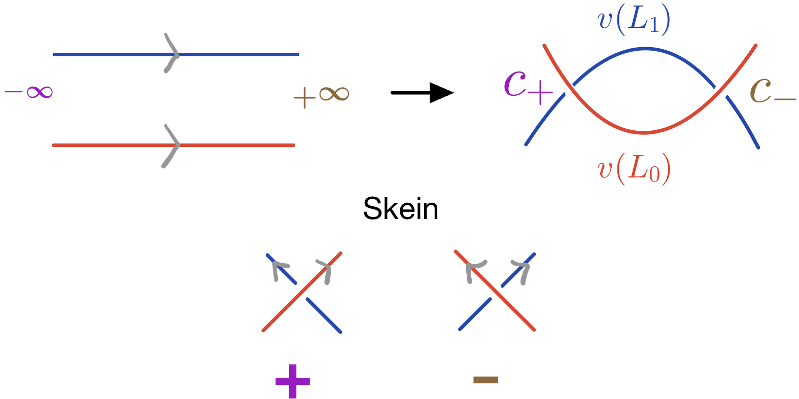
(a) The equivalence of a choice of $\mathbb{Z}/2$-grading with the convention in Skein relations.

(b) The differential counts bigons over that in the base. $\Phi$ is the monodromy.

Figure 4: Grading of points in a bigon

Proof of Lemma 3.16.

Suppose the $v(L_{j})$ are graded by $\phi_{j}^{\mathrm{Hor}}(t):=\frac{1}{\pi}\arg(\dot{\gamma}_{L_{j}}(t))\in(-1/2,1/2)$. Let $\phi_{j,\pm}^{\mathrm{Hor}}:=\phi_{j}^{\mathrm{Hor}}(t_{\pm})$ where $\gamma_{L_{j}}(t_{\pm})=c_{\pm}$. In other words, these are the angles of the tangent vectors to $v(L_{j})$ at the two intersection points $c_{\pm}$. The canonical short paths in the total space are

$$\lambda(t)=\begin{cases}\lambda_{+}(t)=\lambda^{\mathrm{Vert}}_{+}(t)\oplus(dv_{p})^{-1}(e^{-\pi i(1-(\phi^{\mathrm{Hor}}_{1,+}-\phi^{\mathrm{Hor}}_{0,+}))t}\dot{\gamma}_{L_{0}}(t_{+}))&\text{if }p=p_{+}\in Y_{c_{+}},\\ \\ \lambda_{-}(t)=\lambda^{\mathrm{Vert}}_{-}(t)\oplus(dv_{p})^{-1}(e^{-\pi i(\phi^{\mathrm{Hor}}_{0,-}-\phi^{\mathrm{Hor}}_{1,-})t}\dot{\gamma}_{L_{0}}(t_{-}))&\text{if }p=p_{-}\in Y_{c_{-}}\end{cases}$$

where $\lambda^{\mathrm{Vert}}_{\pm}(t)$ are the canonical short paths between fiber Lagrangians over $c_{\pm}$. Note that in $Y_{c_{-}}$ we have an identification of Floer complexes

$$CF(\Phi_{\gamma_{L_{0}}(t_{+})\to\gamma_{L_{0}}(t_{-})}(L_{0,c_{+}}),\Phi_{\gamma_{L_{1}}(t_{+})\to\gamma_{L_{1}}(t_{-})}(L_{1,c_{+}}))\cong CF(\Phi(L_{0,c_{+}}),L_{1,c_{+}})$$ (3.13)

where $(\Phi_{\gamma_{L_{1}}(t_{+})\to\gamma_{L_{1}}(t_{-})})^{-1}\Phi_{\gamma_{L_{0}}(t_{+})\to\gamma_{L_{0}}(t_{-})}=\Phi$ is the monodromy, by applying the diffeomorphism
$(\Phi_{\gamma_{L_{1}}(t_{+})\to\gamma_{L_{1}}(t_{-})})^{-1}$ to both Lagrangians branes on the left Floer complex. Thus by Corollary 3.15, where $\widetilde{\alpha}_{\lambda_{\pm}}^{\mathrm{Hor}}(0)=\widetilde{\alpha}_{v(L_{0})}(c_{\pm})=\phi^{\mathrm{Hor}}_{0,\pm}$ so it cancels out as in Equation (3.11),

$$\deg(\widetilde{L_{0}},\widetilde{L_{1}};p_{+}) =\deg(\widetilde{L_{0,c_{+}}},\widetilde{L_{1,c_{+}}};p_{+})+\deg_{\mathbb{C}}(\widetilde{v(L_{0})},\widetilde{v(L_{1})};c_{+})$$ (3.14)

$$=\deg(\widetilde{L_{0,c_{+}}},\widetilde{L_{1,c_{+}}};p_{+})+(\phi^{\mathrm{Hor}}_{1,+}-\phi^{\mathrm{Hor}}_{0,+})-(-(1-(\phi^{\mathrm{Hor}}_{1,+}-\phi^{\mathrm{Hor}}_{0,+})))$$

$$=\deg(\widetilde{L_{0,c_{+}}},\widetilde{L_{1,c_{+}}};p_{+})+1$$

$$\deg(\widetilde{L_{0}},\widetilde{L_{1}};p^{\prime}_{-}) =\deg({\Phi(\widetilde{L_{0,c_{+}}})},\widetilde{L_{1,c_{+}}};p^{\prime}_{-})+(\phi^{\mathrm{Hor}}_{1,-}-\phi^{\mathrm{Hor}}_{0,-})-(-(\phi^{\mathrm{Hor}}_{0,-}-\phi^{\mathrm{Hor}}_{1,-}))$$

$$=\deg({\Phi(\widetilde{L_{0,c_{+}}})},\widetilde{L_{1,c_{+}}};p^{\prime}_{-}).$$

Although different graded lifts exist $\widetilde{\alpha_{v(L)}}:v(L)\to\mathbb{R}$ for $L=L_{0}$ and $L=L_{1}$, the difference between degrees of $p_{+}$ and $p_{-}$ stays the same. ∎

Remark 3.18.

The bigon may pass through singular fibers, but we only consider the Maslov index of a loop of matrices at an intersection point away from the singular fiber, where we use a decomposition into base and fiber with the globally defined holomorphic $(n+1)$-form that splits into base and fiber terms, above.

Remark 3.19.

Note that the definition of a grading of an intersection point is consistent with the Morse theory interpretation of $J$-holomorphic strips. Morse homology has chain complexes generated by critical points of a Morse function $f$, and the differential counts flow lines of $-\nabla f$. Lagrangian Floer cohomology is Morse cohomology for the action functional measuring negative area $\mathcal{A}(\gamma,[\Gamma])=-\int_{\Gamma}\omega$ for $\gamma$ in the path space $\mathcal{P}(L_{0},L_{1}):=\{\gamma:[0,1]\to Y\mid\gamma(0)\in L_{0},\gamma(1)\in L_{1}\}$ and for equivalence class $[\Gamma]$ of a homotopy $\Gamma:[0,1]\times[0,1]\to\gamma$ between $\gamma$ and a fixed base point in the connected component of $\mathcal{P}(L_{0},L_{1})$ containing $\gamma$, as in [Aur14, p 3]. Critical points are intersection points $L_{0}\cap L_{1}$, and the differential counts flow lines of $\nabla\left(\int_{\Gamma}\omega\right)$, which are $J$-holomorphic strips that flow with increasing signed $(\partial_{s},\partial_{t})$ area for coordinates $(s,t)\in\mathbb{R}\times[0,1]$ on the strip in Figure 4(a). Therefore, since we are considering cohomology instead of Morse homology, the differential goes opposite to the flow direction, and the intersection points are graded accordingly to increase degree by 1 from $p_{-}$ to $p_{+}$. This matches the result in Lemma 3.16. (The flow direction, grading of a Lagrangian, and orientation of a Lagrangian are not directly related.)

References

• [AA] Mohammed Abouzaid and Denis Auroux, Homological mirror symmetry for hypersurfaces in $(\mathbb{C}^{*})^{n}$, https://arxiv.org/abs/2111.06543, to appear in Geometry & Topology.
• [ACLL] Haniya Azam, Catherine Cannizzo, Heather Lee, and Chiu-Chu Melissa Liu, Fukaya category on a symplectic manifold with a B-field, https://arxiv.org/pdf/2311.04143.pdf.
• [AS19] Mohammed Abouzaid and Ivan Smith, Khovanov homology from Floer cohomology, J. Amer. Math. Soc. 32 (2019), no. 1, 1–79. MR 3867999
• [Aur14] Denis Auroux, A beginner’s introduction to Fukaya categories, Contact and symplectic topology, Bolyai Soc. Math. Stud., vol. 26, János Bolyai Math. Soc., Budapest, 2014, pp. 85–136.
• [Can20] Catherine Cannizzo, Categorical mirror symmetry on cohomology for a complex genus 2 curve, Advances in Mathematics 375 (2020), 107392.
• [Gan16] Sheel Ganatra, Math 257b: Topics in symplectic geometry – aspects of Fukaya categories, https://drive.google.com/file/d/1-anqMQbQCxgu01AKCK3rUqmOF95vkhvK/view, 2016.
• [GH94] Phillip Griffiths and Joseph Harris, Principles of algebraic geometry, Wiley Classics Library, John Wiley & Sons, Inc., New York, 1994, Reprint of the 1978 original.
• [GPS22] Sheel Ganatra, John Pardon, and Vivek Shende, Sectorial descent for wrapped Fukaya categories, 2022.
• [MS98] Dusa McDuff and Dietmar Salamon, Introduction to symplectic topology, second ed., Oxford Mathematical Monographs, The Clarendon Press, Oxford University Press, New York, 1998. MR 1698616
• [Sei99] Paul Seidel, Lagrangian two-spheres can be symplectically knotted, J. Differential Geom. 52 (1999), no. 1, 145–171. MR 1743463
• [Sei00]  , Graded Lagrangian submanifolds, Bull. Soc. Math. France 128 (2000), no. 1, 103–149.
• [Sei08]  , Fukaya categories and Picard-Lefschetz theory, Zurich Lectures in Advanced Mathematics, European Mathematical Society (EMS), Zürich, 2008. MR 2441780