Risk-Averse Control of Markov Systems with Value Function Learning

Abstract

We consider a control problem for a finite-state Markov system whose performance is evaluated by a coherent Markov risk measure. For each policy, the risk of a state is approximated by a function of its features, thus leading to a lower-dimensional policy evaluation problem, which involves non-differentiable stochastic operators. We introduce mini-batch transition risk mappings, which are particularly suited to our approach, and we use them to derive a robust learning algorithm for Markov policy evaluation. Finally, we discuss structured policy improvement in the feature-based risk-averse setting. The considerations are illustrated with an underwater robot navigation problem in which several waypoints must be visited and the observation results must be reported from selected transmission locations. We identify the relevant features, we test the simulation-based learning method, and we optimize a structured policy in a hyperspace containing all problems with the same number of relevant points.
Keywords: Dynamic Risk Measures, Reinforcement Learning, Function Approximation, Robot Navigation.

1 Introduction

We consider a Markov decision process (MDP) with a finite state space $\mathcal{X}=\{1,\dots,n\}$, which may be very large, the control space $\mathcal{U}$ (which is finite as well), the feasible control set $U:\mathcal{X}\rightrightarrows\mathcal{U}$, and the controlled transition probability matrix $P_{ij}(u)$, $i,j\in\mathcal{X}$, $u\in U(i)$; its $i$-th row, $P_{i}(u)$, is the distribution of the next state if the current state is $i$ and control is $u$. We use $\pi_{t}$ to denote the decision rule to choose the control $u_{t}$ at time $t=0,1,\dots$, and $\varPi=\{\pi_{0},\pi_{1},\dots\}$ is the policy. In general, $\pi_{t}$ may be a function of $(i_{0},i_{1},\dots,i_{t})$, the states visited at times $0,1,\dots,t$, and produce a probability distribution on $U(i_{t})$, but we shall be mainly concerned with stationary deterministic Markov policies, in which $u_{t}=\pi(i_{t})$ with a stationary (time-invariant) decision rule $\pi$.

For any stationary deterministic Markov policy $\varPi=\{\pi,\pi,\dots\}$, and any initial state $i_{0}$, the sequence of states $\{i_{t}\}_{t=0,1,\dots}$ is a Markov chain, with the transition probability matrix $P^{\pi}$ having entries $P^{\pi}_{ij}=P_{ij}(\pi(i))$. At each time $t=0,1,\dots$, if the state is $i_{t}$ and the control is $u_{t}$, a cost $c(i_{t},u_{t})$ is incurred, where $c:\mathcal{X}\times\mathcal{U}\to\mathbb{R}$. Thus, under a Markov policy $\varPi$, the resulting sequence of costs is $c^{\pi}(i_{t})=c(i_{t},\pi_{t}(i_{t}))$, $t=0,1,\dots$. In standard formulations (see, e.g., Puterman (1994); Bertsekas (2017)), the objective is to find a control policy that minimizes or maximizes the expected (discounted) sum or the expected average of stage-wise costs or rewards over a finite or infinite horizon.

Our goal is to use a dynamic measure of risk to evaluate the MDP’s performance. The general theory of dynamic risk is discussed, inter alia, in Scandolo (2003); Cheridito et al. (2006); Ruszczyński and Shapiro (2006); Artzner et al. (2007); Pflug and Römisch (2007); Shapiro et al. (2021) and the references therein. Our approach uses Markov dynamic risk measures introduced in Ruszczyński (2010), and further developed in Shen et al. (2013); Lin and Marcus (2013); Çavus and Ruszczyński (2014a, b); Fan and Ruszczyński (2018); Fan and Ruszczyński (2022); Bäuerle and Glauner (2022). In this theory, one obtains risk-averse versions of the Bellman equation, which are difficult to solve because of the nonlinear and nonsmooth nature of the risk measures and because of the size of the state space. To deal with this difficulty, we are using value function approximation, in the spirit of Sutton (1988); Bradtke and Barto (1996); Tsitsiklis and Roy (1997); Sutton and Barto (1998); Melo and Ribeiro (2007); Yang and Wang (2020); Jin et al. (2020), and many references therein. However, because of the nonlinear dependence of risk on the probability measure, these approaches are not directly applicable in our case.

Several works introduce models of risk into reinforcement learning: exponential utility functions (Borkar, 2001, 2002; Basu et al., 2008; Fei and Xu, 2022) and mean-variance models (Tamar et al., 2012; Prashanth and Ghavamzadeh, 2014). A few later studies propose heuristic approaches involving specific coherent risk measures, such as CVaR in the objective or constraints (Chow and Ghavamzadeh, 2014; Chow et al., 2017; Ma et al., 2018). Generative model value iteration with coherent measures was analyzed by Yu et al. (2018). Risk-aware Q-learning with Markov risk measures is considered by Huang and Haskell (2017). A risk-averse policy gradient method was considered in Ma et al. (2017). All these methods apply to problems with a small number of state-action pairs allowing exhaustive experimentation.

Value function approximations in the context of distributionally robust MDPs were considered by Tamar et al. (2014). Ref. Tamar et al. (2017) studies the policy gradient approach for Markov risk measures and use it in an actor-critic type algorithm. Both approaches are heuristic. Policy evaluation with linear architecture and Markov risk measures by a method of temporal differences was analyzed by Köse and Ruszczyński (2021), and asymptotic convergence was proved. The recent work of Yin et al. (2022) uses variance to control the value iteration procedure. Recently, Lam et al. (2023) proposed a version of a risk-aware reinforcement learning method with coherent risk measures and function approximation. However, at each iteration, it uses extensive experimentation (double sampling) to statistically estimate the risk with high accuracy and high probability at each state-control pair.

In section 2, we briefly outline the main results of the theory of Markov risk measures and the resulting dynamic programming techniques. In section 3, we introduce a new class of recursive Markov risk measures based on mini-batch transition risk mappings and study their properties. In section 4, we use them to develop a policy evaluation method by simulation. We also propose a parametric policy improvement scheme based on the evaluations. Finally, in section 5, we discuss the applications of these methods to the challenging problem of underwater robot navigation.

2 Markov Risk Measures

Consider a finite-horizon setting first. Suppose the actions are generated by a deterministic policy $\varPi$. A dynamic risk measure evaluates the sequence of the random costs $Z_{t}=c(i_{t},u_{t})$, $t=0,1,\dots,T-1$ and $Z_{T}=c_{T}(i_{T})$ in a risk-aware fashion. We denote by $\mathcal{Z}_{t}$ the space of all real functions of the history $\{i_{0},\dots,i_{t}\}$. Because of the need to evaluate future costs at any period, a dynamic risk measure is a collection of conditional risk measures $\rho_{t,T}:\mathcal{Z}_{t}\times\dots\times\mathcal{Z}_{T}\to\mathcal{Z}_{t}$, $t=0,1,\dots,T$, for which we postulate three properties:

• $\rho_{t,T}(0,\dots,0)=0$;

• If $(Z_{t},\dots,Z_{T})\leq(W_{t},\dots,W_{T})$, then $\rho_{t,T}(Z_{t},\dots,Z_{T})\leq\rho_{t,T}(W_{t},\dots,W_{T})$;

• $\rho_{t,T}(Z_{t},\dots,Z_{T})=Z_{t}+\rho_{t,T}(0,Z_{t},\dots,Z_{T})$.

Here and below, all inequalities are understood component-wise.

Fundamental for such a nonlinear dynamic cost evaluation is time consistency, discussed in various forms by Cheridito et al. (2006); Artzner et al. (2007); Ruszczyński (2010); Cheridito and Kupper (2011): A dynamic risk measure is time consistent if for every $t=0,1,\dots,T-1$, if $Z_{t}=W_{t}$ and $\rho_{t+1,T}(Z_{t+1},\dots,Z_{T})\leq\rho_{t+1,T}(W_{t+1},\dots,W_{T})$, then $\rho_{t,T}(Z_{t},\dots,Z_{T})\leq\rho_{t,T}(W_{t},\dots,W_{T})$. As proved by Ruszczyński (2010), such measures, under the conditions specified above, must have the recursive form:

$$\rho_{t,T}(Z_{t:T})=Z_{t}+\rho_{t}\Big{(}Z_{t+1}+\rho_{t+1}\big{(}Z_{t+2}+\dots+\rho_{T-1}(Z_{T})\cdots\big{)}\Big{)},$$

where each $\rho_{t}(\cdot)$ is a one-step conditional risk measure. This formula, generalizing the tower property of conditional expectations, is pertinent to our approach.

Markov risk measures evaluate the risk-adjusted value of future costs $(Z_{t},\dots,Z_{T})$ in a Markov system with a Markov control policy $u_{t}=\pi_{t}(i_{t})$, $t=0,1,\dots,T-1$, in such a way that the value of the future cost sequence is a function of the current state: $\rho_{t,T}(Z_{t},\dots,Z_{T})=v_{t,T}^{\pi}(i_{t})$, where $v_{t,T}^{\pi}\in\mathcal{V}=\mathbb{R}^{n}$. This, combined with the properties specified above, implies that transition risk mappings $\sigma_{t,i}:\mathcal{P}(\mathcal{X})\times\mathcal{V}\to\mathbb{R}$, $t=0,1,\dots,T-1$, exist such that the value of each state for the Markovian policy $\pi$ can be evaluated by the following procedure:

$$v_{t,T}^{\pi}(i) =c(i,\pi_{t}(i))+\sigma_{t,i}\big{(}P_{i}^{\pi_{t}},v^{\pi}_{t+1,T}\big{)},\quad i\in\mathcal{X},\quad t=0,1,\dots,T-1;$$ (1)

$$v_{T,T}^{\pi}(i) =c_{T}(i),\quad i\in\mathcal{X};$$

see (Ruszczyński, 2010; Fan and Ruszczyński, 2022) for the detailed derivation. The first argument of $\sigma_{t,i}(\cdot,\cdot)$ is a probability measure on $\mathcal{X}$ (an element of the simplex in $\mathbb{R}^{n}$). The space of these measures is denoted by $\mathcal{P}(\mathcal{X})$. We use the subscript $(t,T)$ for the value function because we shall increase $T$ to infinity in due course.

One may remark here that the risk-neutral model is a special case of (1), with the bilinear $\sigma_{t,i}\big{(}P^{\pi}_{i},v^{\pi}_{t+1,T}\big{)}=P^{\pi}_{i}v^{\pi}_{t+1,T}$, but we are interested in mappings that depend on $P^{\pi}_{i}$ and on $v^{\pi}_{t+1,T}$ in a nonlinear way.

In the infinite-horizon case, we consider the sequence of discounted costs $Z_{t}=\alpha^{t-1}c^{\pi}(i_{t})$, $t=0,1,\dots$, with some discount factor $\alpha\in(0,1)$. We also assume that the transition risk mappings are stationary (do not depend on $t$) and satisfy the axioms of a coherent measure of risk Artzner et al. (1999):

• $\sigma_{i}(P_{i},\lambda v+(1-\lambda)w)\leq\lambda\sigma_{i}(P_{i},v)+(1-\lambda)\sigma_{i}(P_{i},w)$, $\forall\,\lambda\in[0,1]$, $\forall\,v,w\in\mathcal{V}$;

• If $v\leq w$ (componentwise) then $\sigma_{i}(P_{i},v)\leq\sigma_{i}(P_{i},w)$;

• $\sigma_{i}(P_{i},v+\beta\mathds{1})=\sigma_{i}(P_{i},v)+\beta$, for all $\beta\in\mathbb{R}$ (here, $\mathds{1}$ is a vector of 1’s);

• $\sigma_{i}(P_{i},\alpha v)=\alpha\sigma_{i}(P_{i},v)$, for all $\alpha\geq 0$.

Then, as demonstrated in Ruszczyński (2010), the infinite-horizon discounted risk measure,

$$v^{\pi}(i)\mathrel{\overset{\raisebox{-0.20004pt}{$\scriptstyle\vartriangle$}}{\,=\,}}\lim_{T\to\infty}v^{\pi}_{0,T}(i),\quad i\in\mathcal{X},$$

is well-defined and satisfies the risk-averse policy evaluation equation:

$$v^{\pi}(i)=c^{\pi}(i)+\alpha\sigma_{i}\big{(}P^{\pi}_{i},v^{\pi}(\cdot)\big{)},\quad i\in\mathcal{X}.$$ (2)

In the vector form, we can write

$$v^{\pi}=c^{\pi}+\alpha\vec{\sigma}\big{(}P^{\pi},v^{\pi}\big{)},$$ (3)

with the mapping $\vec{\sigma}\big{(}P^{\pi},v^{\pi}\big{)}=\big{\{}\sigma_{i}\big{(}P^{\pi}_{i},v^{\pi}(\cdot)\big{)}\big{\}}_{i\in\mathcal{X}}$. Furthermore, the optimal value function $v^{*}(\cdot)$ satisfies the dynamic programming equation

$$v^{*}(i)=\min_{u\in U(i)}\big{\{}c(i,u)+\alpha\sigma_{i}\big{(}P_{i}^{u},v^{*}(\cdot)\big{)}\big{\}},\quad i\in\mathcal{X},$$ (4)

and the deterministic Markov policy defined by the minimizers above is the best among all history-dependent policies. The Reader is referred to Ruszczyński (2010); Fan and Ruszczyński (2022); Bäuerle and Glauner (2022) for the detailed derivation of these equations, for much more general state and control spaces.

Remark 2.1.

In MDP’s in which the stage-wise costs at $t=1,\dots,T-1$ depend on the current state $i_{t}$, current control $u_{t}$, and the next state $i_{t+1}$, via a function $c:\mathcal{X}\times\mathcal{U}\times\mathcal{X}\to\mathbb{R}$, and the terminal cost is $c_{T}(x_{T})$, the policy evaluation equation (1) takes on the form:

$$v^{\pi}_{t,T}(i)=\sigma_{i}\big{(}P^{\pi}_{i},c(i,\pi_{t}(i),\cdot)+\alpha v^{\pi}_{t+1,T}(\cdot)\big{)},\ i\in\mathcal{X},\ t=1,\dots,T-1;$$

the final value is $v^{\pi}_{T,T}(i)=c_{T}(i)$, as before. Accordingly, the infinite horizon stationary Markov policy evaluation equation (2) and the dynamic programming equation (4) are:

$$v^{\pi}(i) =\sigma_{i}\big{(}P^{\pi}_{i},c(i,\pi(i),\cdot)+\alpha v^{\pi}(\cdot)\big{)},\quad i\in\mathcal{X},$$

$$v^{*}(i) =\min_{u\in U(i)}\sigma_{i}\big{(}P^{u}_{i},c(i,u,\cdot)+\alpha v^{*}(\cdot)\big{)},\quad i\in\mathcal{X},$$

respectively.

Remark 2.2.

The derivations that lead to the policy evaluation equation (2) and the dynamic programming equation (4) are heavily dependent on the assumptions that the dynamic measure of risk is time-consistent and Markovian. An alternative approach is to consider an overall risk measure of the total cost: $\varrho\big{(}\sum_{t=0}^{\infty}\alpha^{t}c(i_{t},u_{t})\big{)}$. For some specific measures of risk $\varrho(\cdot)$, such as the Average Value at Risk, dynamic programming relations may be derived with the use of additional state variables; see Bäuerle and Ott (2011); Uğurlu (2017); Ding and Feinberg (2022).

Eq. (4) can be solved, in principle, by the risk-averse versions of the value iteration method or the policy iteration method, which we quickly review below. After evaluating a policy $\pi^{k}$ by (2), we use the right-hand side of (4) to find the next policy:

$$\pi^{k+1}(i)=\mathop{\text{argmin}}_{u\in U(i)}\big{\{}c(i,u)+\alpha\sigma_{i}\big{(}P_{i}^{u},v^{\pi^{k}}(\cdot)\big{)}\big{\}},\quad i\in\mathcal{X};$$ (5)

the method stops when $\pi^{k}(i)$ is an equally good solution of (5) for all $i$, and thus $v^{\pi^{k}}$ satisfies (4). The main difficulty is the implementation of this method when the state space is very large.

In addition to the axioms of a coherent measure of risk, we shall impose additional conditions on the transition risk mappings involving their dependence on the probability measure. For two pairs $(P,v)$ and $(Q,w)$ the notation $(P,v){\sim}(Q,w)$ means that $P\{v\leq\eta\}=Q\{w\leq\eta\}$ for all $\eta\in\mathbb{R}$ (both models have identical distribution functions). We postulate two natural properties of a transition risk mapping.

• If $(P_{i},v){\sim}(Q_{i},w)$ then $\sigma_{i}(P_{i},v)=\sigma_{i}(Q_{i},w)$;

• $\sigma_{i}(P_{i},v)=\sigma_{i}(P_{i},\mathds{1}_{\mathop{\textup{supp}}(P_{i})}v)$.

The symbol $\mathds{1}_{\mathop{\textup{supp}}(P_{i})}$ denotes the characteristic function of the support set of $P_{i}$. The support property means that only these values $v(j)$ matter, for which a transition to state $j$ is possible. It is automatic for the expected value but needs to be required for general operators. An example is the mean–semideviation mapping Ogryczak and Ruszczyński (1999):

$$\sigma_{i}(P_{i},v)=\sum_{j\in\mathcal{X}}P_{ij}v(j)+c\sum_{j\in\mathcal{X}}P_{ij}\Big{[}v(j)-\sum_{k\in\mathcal{X}}P_{ik}v(k)\Big{]}_{+},$$ (6)

with $c\in[0,1]$. Another example is the Average Value at Risk (Ogryczak and Ruszczyński (2002); Rockafellar and Uryasev (2002)):

$$\sigma_{i}(P_{i},v)=\min_{\eta\in\mathbb{R}}\big{\{}\eta+\frac{1}{\alpha}\sum_{j\in\mathcal{X}}P_{ij}\max(0,v(j)-\eta)\big{\}},\quad\alpha\in(0,1].$$ (7)

Yet another example, rarely used in the risk measure theory and practice, due to its conservative nature, but very relevant for us, is the worst-case mapping:

$$\sigma_{i}(P_{i},v)=\max\big{\{}v(j):P_{ij}>0,\ j\in\mathcal{X}\big{\}}.$$ (8)

All examples above are coherent and law-invariant risk mappings having the support property.

The main difficulty associated with these and other mappings derived from coherent measures of risk is their statistical estimation.

3 Mini-Batch Transition Risk Mappings

We now propose a class of transition risk mappings that are more amenable to statistical estimation.

Suppose $\sigma_{i}:\mathcal{P}(\mathcal{X})\times\mathcal{V}\to\mathbb{R}$ is a transition risk mapping. If we draw a sample $j^{1:N}=(j^{1},\dots,j^{N})$, with $N$ independent components distributed according to $P_{i}$ in $\mathcal{X}$, we obtain a random empirical measure on $\mathcal{X}$: $P^{(N)}(j^{1:N})=\frac{1}{N}\sum_{m=1}^{N}\delta_{j^{m}}$, where $\delta_{j}$ represents the unit mass concentrated at $j$. It is a $\mathcal{P}(\mathcal{X})$-valued random variable on the product space $\mathcal{X}^{N}$ with the product measure $(P_{i})^{N}$. Using it as the argument of $\sigma_{i}$, we obtain a random transition risk mapping $\sigma_{i}\big{(}P^{(N)}(j^{1:N}),v\big{)}$. Finally, we define

$$\sigma_{i}^{(N)}(P_{i},v)=\mathbb{E}_{j^{1:N}\sim(P_{i})^{N}}\big{\{}\sigma_{i}\big{(}P^{(N)}(j^{1:N}),v\big{)}\big{\}}.$$ (9)

We call it the mini-batch transition risk mapping.

A simple example is the mini-batch transition risk mapping derived from (8):

$$\sigma_{i}^{(N)}(P_{i},v)=\mathbb{E}_{j^{1:N}\sim(P_{i})^{N}}\Big{[}\max_{1\leq m\leq N}v(j^{m})\Big{]}.$$ (10)

We can also derive a mini-batch version of (6) or (7). For example, the mini-batch Average Value at Risk has the following form:

$$\sigma_{i}^{(N)}(P_{i},v)=\mathbb{E}_{j^{1:N}\sim(P_{i})^{N}}\Big{[}\min_{\eta\in\mathbb{R}}\big{\{}\eta+\frac{1}{\alpha N}\sum_{m\in\mathcal{X}}\max(0,v(j^{m})-\eta)\big{\}}\Big{]}.$$ (11)

It is evident that we may mix the mini-batch risk mappings with the expected value, obtaining

$$\sigma_{i}(P_{i},v)=(1-c)\mathbb{E}_{j^{1:N}\sim(P_{i})^{N}}\bigg{[}\frac{1}{N}\sum_{m=1}^{N}v(j^{m})\bigg{]}+c\sigma_{i}^{(N)}(P_{i},v),\quad c\in[0,1].$$ (12)

The following observation proves that the mini-batch versions inherit the properties of the “base” risk measures.

Lemma 3.1.

If the transition risk mapping $\sigma_{i}(\cdot,\cdot)$ is convex (monotonic, translation equivariant, positively homogeneous, has the support property, or is law invariant) then the mini-batch transition risk mapping $\sigma_{i}^{(N)}(\cdot,\cdot)$ has the corresponding property as well.

Proof.

The first five properties are evident; only the law invariance requires proof. Consider two pairs: $\big{(}\frac{1}{N}\sum_{m=1}^{N}\delta_{j^{m}},v\big{)}$ and $\big{(}\frac{1}{N}\sum_{m=1}^{N}\delta_{k^{m}},w\big{)}$. If, for some permutation $\lambda$ of $\{1,\dots,N\}$,

$$\big{(}v(j^{1}),\dots,v(j^{N})\big{)}=\big{(}w(k^{\lambda(1)}),\dots,w(k^{\lambda(N)})\big{)},$$

then the two pairs have identical distribution functions. By the law invariance of $\sigma_{i}(\cdot,\cdot)$, we have$\sigma_{i}\big{(}\frac{1}{N}\sum_{m=1}^{N}\delta_{j^{m}},v\big{)}=\sigma_{i}\big{(}\frac{1}{N}\sum_{m=1}^{N}\delta_{k^{m}},w\big{)}$. Thus a measurable function $\varPsi:\mathbb{R}^{N}\to\mathbb{R}$ exists, such that

$$\sigma_{i}(P_{i}^{(N)},v)=\varPsi\big{(}v(j^{1}),\dots,v(j^{N})\big{)},$$

and for every permutation $\lambda$ of $\{1,\dots,N\}$, $\varPsi\big{(}v(j^{1}),\dots,v(j^{N})\big{)}=\varPsi\big{(}v(j^{\lambda(1)}),\dots,v(j^{\lambda(N)})\big{)}$. Now, if $(P_{i},v)\sim(Q_{i},w)$, then for $j^{1:N}\sim P_{i}^{N}$ and $k^{1:N}\sim Q_{i}^{N}$, the vectors $\big{(}v(j^{1}),\dots,v(j^{N})\big{)}$ and $\big{(}w(k^{1}),\dots,w(k^{N})\big{)}$ have the same distribution. Therefore,

$$\sigma_{i}^{(N)}(P_{i},v) =\mathbb{E}_{j^{1:N}\sim P_{i}^{N}}\big{\{}\varPsi\big{(}v(j^{1}),\dots,v(j^{N})\big{)}\big{\}}$$

$$=\mathbb{E}_{k^{1:N}\sim Q_{i}^{N}}\big{\{}\varPsi\big{(}w(k^{1}),\dots,w(k^{N})\big{)}\big{\}}=\sigma_{i}^{(N)}(Q_{i},w),$$

which verifies the law invariance. ∎

4 Policy Evaluation with Risk Approximation

If the state space $\mathcal{X}$ is very large, it is impossible to tabulate the function $v^{\pi}(\cdot)$. Instead, we use an approximation

$$v(i)\approx\tilde{v}(i)\triangleq f(\varPhi_{i};\theta),\quad i\in\mathcal{X},$$

of $M\ll n$ features $\varPhi_{i}=\big{[}\varPhi_{i,1},\dots,\varPhi_{i,M}\big{]}$, $i\in\mathcal{X}$, and an identical learning model $f:\mathbb{R}^{M}\times\mathbb{R}^{d}\to\mathbb{R}$ with parameters $\theta\in\mathbb{R}^{d}$, where $d\ll n$.

Compactly, $\tilde{v}=F(\varPhi;\theta)$, with the diagonal structure: $F_{i}(\varPhi;\theta)=f(\varPhi_{i};\theta)$, $i\in\mathcal{X}$. An important special case is the linear model:

$$\tilde{v}=\varPhi\theta,$$ (13)

in which $M=d$. Thus, $\tilde{v}(i)=\varPhi_{i}\theta$, $i\in\mathcal{X}$.

Such an approach is widespread in the reinforcement learning literature. The linear value function approximation approaches to MDPs have a long history; see Bradtke and Barto (1996); Sutton (1988); Tsitsiklis and Van Roy (1997); Sutton and Barto (1998); Melo and Ribeiro (2007) and many references therein. The concept of a linear (mixture) MDP Bradtke and Barto (1996); Melo and Ribeiro (2007), originating from the theory of linear bandits (Bubeck et al., 2012; Lattimore and Szepesvári, 2020), is pertinent in this setting. It has been recently used by Ayoub et al. (2020); Yang and Wang (2020); Jin et al. (2020); Modi et al. (2020) to develop complexity bounds for expected value RL algorithms. The generalization to bilinear models by Du et al. (2021) extends the applicability of this class. The state aggregation or lumping approaches of Dong et al. (2019); Katehakis and Smit (2012) are also related to this model. Our intention is to extend the value approximation approach to the risk-averse case.

4.1 Abstract Policy Evaluation

Suppose the initial state $i_{1}$ is random, with probability distribution $P_{0}$. If the Markov chain created by the policy $\pi$ is an unichain, we denote by $q^{\pi}$ its stationary distribution. If the chain is absorbing, as in our application in section 5, we consider its restarted version, with the new transition probabilities $P_{0}$ at each absorbing state. If we exclude the periodic case, it becomes an unichain again.

As in the expected value case, we need to project the right-hand side of the risk-averse policy evaluation equation (3) on the set in which the left-hand side lives. Therefore, we define the operator:

$$D^{\pi}(v)=\operatorname{\textrm{P}roj}_{\mathcal{R}}^{\pi}\big{(}c^{\pi}+{\alpha}\vec{\sigma}(P^{\pi},v)\big{)},\quad v\in\mathcal{V},$$ (14)

where $\mathcal{R}=\mathop{\textrm{range}}(F(\varPhi;\cdot))$, $\operatorname{\textrm{P}roj}_{\mathcal{R}}^{\pi}(w)=\mathop{\text{argmin}}_{v\in\mathcal{R}}{\|v-w\|}_{q^{\pi}}^{2}$, and the norm $\|v\|^{2}_{q}=\sum_{i\in\mathcal{X}}q_{i}v(i)^{2}$. The operator $\operatorname{\textrm{P}roj}_{\mathcal{R}}^{\pi}(\cdot)$ is well-defined if the set $\mathcal{R}$ is convex and closed, which we shall assume from now on.

The projected risk-averse policy evaluation equation has the form:

$$\tilde{v}^{\pi}=D^{\pi}(\tilde{v}^{\pi}).$$ (15)

To establish relevant properties of (14), we use the dual representation of a coherent measure of risk Ruszczyński and Shapiro (2006), which in our case can be stated as follows. For every $i\in\mathcal{X}$, a convex, closed and bounded set $A_{i}(P_{i})\subset\mathcal{P}(\mathcal{X})$ exists, such that $\sigma_{i}(P_{i},v)=\max_{\mu_{i}\in A_{i}(P_{i})}\mu_{i}v$, $v\in\mathcal{V}$.

Lemma 4.1.

The operator $D^{\pi}$ is Lipschitz continuous in the $q^{\pi}$-norm with the modulus $\alpha\sqrt{1+\varkappa}$, where

$$\varkappa=\max\bigg{\{}\frac{|\mu_{ij}-p_{ij}|}{p_{ij}}:\mu_{i}\in A_{i}(P_{i}),p_{ij}>0,i,j\in\mathcal{X}\bigg{\}},$$

is the distortion coefficient.

The proof follows the proof of (Köse and Ruszczyński, 2021, Lem. 1), using the fact that $\operatorname{\textrm{P}roj}_{\mathcal{R}}^{\pi}(\cdot)$ is a nonexpansive mapping in the norm $\|\cdot\|_{q^{\pi}}$.

To evaluate the policy by equation (15), we can thus (theoretically) apply a fixed point algorithm. We define the minimizing objective with respect to a reference point $\bar{\theta}$:

$$L_{\bar{\theta}}(\theta) =\big{\|}F(\varPhi;\theta)-c^{\pi}-\alpha\vec{\sigma}\big{(}P^{\pi},F(\varPhi;\bar{\theta})\big{)}\big{\|}_{q}^{2}$$ (16)

$$=\mathbb{E}_{i\sim q^{\pi}}\Big{\{}\big{[}f(\varPhi_{i};\theta)-c_{i}^{\pi}-\alpha\sigma_{i}\big{(}P_{i}^{\pi},F(\varPhi;\bar{\theta})\big{)}\big{]}^{2}\Big{\}},$$

and we iterate

$$\theta^{\ell+1}=\mathop{\text{argmin}}L_{\theta^{\ell}}(\theta),\quad\ell=1,2,\dots.$$ (17)

Theorem 4.2.

If the set $\mathcal{R}$ is convex and closed and $\alpha\sqrt{1+\varkappa}<1$, then the sequence of functions $\tilde{v}^{\ell}=F(\varPhi;\theta^{\ell})$, $\ell=1,2\dots$, is convergent linearly to the unique solution of the equation (15).

Proof.

In the function space $\mathcal{V}$, the algorithm (17) has the form $\tilde{v}^{\ell+1}=D^{\pi}(\tilde{v}^{\ell})$, $\ell=1,2,\dots$. Its linear convergence follows from the contraction property of the operator $D^{\pi}$ established in Lemma 4.1. ∎

Evidently, if $F(\varPhi\,;\,\cdot\,)$ is an injection, then the sequence $\{\theta^{\ell}\}_{\ell\geq 1}$ is convergent as well.

However, the practical implementation of the abstract scheme (17) is extremely difficult. The objective function (16) is the expected value with respect to the stationary distribution $q^{\pi}$. Furthermore, the values of the stage-wise transition risk mapping ${\sigma}\big{(}P_{i}^{\pi},F(\varPhi;\bar{\theta})\big{)}$ are not observed, and their estimation would require extensive sampling from the conditional distribution. All these difficulties make the scheme (17) difficult to implement in its general form.

4.2 The Risk-Averse Method of Temporal Differences

Another possibility, well-developed in the expected value case, is the application of the method of temporal differences Sutton (1988). It uses differences between the values of the approximate value function at successive states to improve the approximation, concurrently with the evolution of the system. The methods of temporal differences have been proven to converge in the mean (to some limit) in (Dayan, 1992) and almost surely by several studies, with different degrees of generality and precision (Peng, 1993; Dayan and Sejnowski, 1994; Tsitsiklis, 1994; Jaakkola et al., 1994). Almost sure convergence of the stochastic method with linear function approximation to a solution of a projected dynamic programming equation was proved by Tsitsiklis and Van Roy (1997).

The risk-averse method of temporal differences, due to Köse and Ruszczyński (2021), is based on two additional assumptions:

• The feature model is linear, that is, it has the form (13);

• Unbiased statistical estimates $\widetilde{\sigma}_{i}\big{(}P_{i}^{\pi},\varPhi\theta\big{)}$ of the transition risk mappings are available, satisfying

  $$\mathbb{E}\big{[}\widetilde{\sigma}_{i}\big{(}P_{i}^{\pi},\varPhi\theta\big{)}\,\big{|}\,i\big{]}={\sigma}_{i}\big{(}P_{i}^{\pi},\varPhi\theta\big{)}.$$ (18)

If we simulate a trajectory $\{i_{t}\}_{t\geq 0}$ of the system under the policy $\pi$, at each time step $t$, having some estimates $\theta_{t}$ of the model coefficients, we can define the risk-averse temporal differences:

$$d_{t}=\varPhi_{i_{t}}\theta_{t}-c^{\pi}_{i_{t}}-\alpha\sigma_{i_{t}}(P_{i_{t}}^{\pi},\varPhi\theta_{t}),\quad t=0,1,2,\dots.$$ (19)

These are the quantities under the square on the right-hand side of (16) at $\theta=\bar{\theta}=\theta_{t}$.

The temporal differences cannot be easily computed or observed; this would require the evaluation of the risk $\sigma_{i_{t}}(P_{i_{t}}^{\pi},\varPhi\theta_{t})$ and thus consideration of all possible transitions from state $i_{t}$. Instead, we use their random estimates $\widetilde{\sigma}_{i_{t}}(P_{i_{t}}^{\pi},\varPhi\theta_{t})$, and define the observed risk-averse temporal differences,

$$\widetilde{d}_{t}=\varPhi_{i_{t}}\theta_{t}-c^{\pi}_{i_{t}}-\alpha\widetilde{\sigma}_{i_{t}}(P_{i_{t}}^{\pi},\varPhi\theta_{t}),\quad t=0,1,2,\dots.$$ (20)

This allows us to construct the risk-averse temporal difference method as follows:

$$\theta_{t+1}=\theta_{t}-\gamma_{t}\varPhi_{i_{t}}^{\top}\,\widetilde{d}_{t},\quad t=0,1,2,\dots,$$ (21)

with appropriately chosen stepsizes $\gamma_{t}>0$ decreasing to 0. It has been proved in Köse and Ruszczyński (2021) that under the assumptions of Theorem 4.2 and standard conditions on the sequence of stepsizes $\{\gamma_{t}\}_{t\geq 0}$, the sequence of functions $\{\varPhi\theta_{t}\}_{t\geq 0}$ is convergent a.s. to the solution of the projected policy evaluation equation (15).

The mini-batch transition risk mappings (9) provide a convenient tool to construct the statistical estimates $\widetilde{\sigma}_{i}\big{(}P_{i}^{\pi},\varPhi\theta\big{)}$. Suppose that the original transition risk mapping is defined as (9), with some base measure of risk $\hat{\sigma}$:

$$\sigma_{i}(P_{i}^{\pi},\varPhi\theta)=\mathbb{E}_{j^{1:N}\sim(P_{i}^{\pi})^{N}}\big{\{}\hat{\sigma}_{i}\big{(}P^{(N)}(j^{1:N}),\varPhi\theta\big{)}\big{\}}.$$

As it is defined as an expected value, the estimator

$$\widetilde{\sigma}_{i_{t}}(P_{i_{t}}^{\pi},\varPhi\theta_{t})\triangleq\hat{\sigma}_{i}\big{(}P^{(N)}(j^{1:N}),\varPhi\theta\big{)}$$

is an unbiased estimator of the transition risk which can be used in the method of temporal differences. Its calculation involves a small number $N$ is simulations of transitions from the state $i$, and the evaluation of a simple finite-sample risk $\hat{\sigma}_{i}\big{(}P^{(N)}(j^{1:N}),\varPhi\theta\big{)}$ at the simulated successor states $j^{1},\dots j^{N}$.

Consider the application of the mini-batch transition risk mapping (10) with $N=2$ for the risk evaluation. For the convergence of the value iteration method (17) or the method of temporal differences (21), it is essential to estimate its distortion coefficient.

Lemma 4.3.

The distortion coefficient of the mini-batch transition risk mapping (10) with $N=2$ satisfies the inequality

$$\varkappa\leq\max\big{\{}1-p_{ij}:p_{ij}>0\big{\}}<1.$$ (22)

Proof.

Suppose, for simplicity, that the states $j$ such that $p_{ij}>0$ are $\{1,2,\dots,k\}$ and they are ordered in such a way that $v_{1}<v_{2}<\dots<v_{k}$. At such a point $v$, the risk measure ${\sigma}(P^{(2)}(j^{1:2}),\cdot)$ is locally linear. By construction, the distribution function of ${\sigma}(P^{(2)}(j^{1:2}),v)$ has the form

$$P_{j^{1:2}\sim P_{i}^{2}}\big{[}\max_{1\leq m\leq 2}v(j^{m})\leq b\big{]}=\Big{(}P_{j\sim P_{i}}\big{[}v(j)\leq b\big{]}\Big{)}^{2},\quad b\in\mathbb{R}.$$

It follows that the jumps of the distribution function have the sizes

$$\mu_{ij}=\bigg{(}\sum_{s=1}^{j}p_{is}\bigg{)}^{2}-\bigg{(}\sum_{s=1}^{j-1}p_{is}\bigg{)}^{2}=2p_{ij}\sum_{s=1}^{{j}-1}p_{is}+p_{ij}^{2}.$$

Therefore $p_{ij}^{2}\leq\mu_{ij}\leq 2p_{ij}-p_{ij}^{2}$. Subtracting $p_{j}$ and dividing by it, we obtain the estimate (22). The validity of the bound at the points of nondifferentiability of ${\sigma}(P^{(2)}(j^{1:2}),\cdot)$ follows from the fact that the subdifferential at any $v$ is the convex hull of limits of gradients at points $v^{\prime}$ of differentiability, convergent to $v$. ∎

If we combine the mini-batch risk measure $\sigma^{(2)}(P_{i},v)$ with the expected value, with coefficients $c$ and $1-c$, respectively, we shall obtain $\varkappa\leq c$ (recall that $c\in[0,1]$). Therefore, we can easily satisfy the contraction mapping condition of Theorem 4.2 by choosing $c$ such that $\alpha\sqrt{1+c}<1$. Similar calculations can be carried out for $N>2$.

4.3 Multi-Episodic Least-Squares Policy Evaluation

The policy evaluation problem in (17) for the linear architecture model (13) has the form:

$$\min_{\theta}\,{L}(\theta)\mathrel{\overset{\raisebox{-0.20004pt}{$\scriptstyle\vartriangle$}}{\,=\,}}\mathbb{E}\big{[}\varPhi_{i}\theta-c(i)-\alpha{\sigma}_{i}\big{(}P_{i},\varPhi{\theta^{\ell-1}}\big{)}\big{]}^{2};$$ (23)

the expectation is with respect to the stationary distribution $q^{\pi}$ of the state $i$. The next parameter value $\theta^{\ell+1}$ is the solution of (23).

As we have already mentioned, three difficulties are associated with the problem (23): it involves the enumeration of all states, the stationary distribution $q^{\pi}$ is not known, and the risk mappings $\sigma_{i}(P_{i},\tilde{v})$ cannot be evaluated exactly. To address the first two difficulties, we sample many trajectories of the system operating under the policy $\pi$ (episodes), and we use the empirical distributions as approximations of the stationary distribution. The last difficulty is dealt with by using a mini-batch transition risk mapping $\sigma_{i}^{(N)}(P_{i},\tilde{v})$ for $\sigma_{i}(P_{i},\tilde{v})$ and applying its unbiased estimates $\widetilde{\sigma}_{i}^{(N)}(P_{i},\tilde{v})={\sigma}_{i}\big{(}P^{(N)}(j^{1:N}),\tilde{v}\big{)}$ at the states encountered in the episode simulation.

Below, we outline the method with one episode per iteration, but identical considerations apply to the multi-episodic setting. In the iteration $\ell$ of the method, for a fixed policy $\pi$, we simulate an episode with depth $T_{\ell}$; it begins with a reset state $s^{\ell}_{0}$ (sampled from some distribution $P_{0}$), and ends with a state $s^{\ell}_{T_{\ell}}$. We denote the state at time $t$ of episode $\ell$ by $s^{\ell}_{t}$. At each such state, we simulate $N$ possible successor states ${j}_{\ell,t+1}^{1:N}$ from the transition probability $P_{s^{\ell}_{t}}$ (we write $P$ instead of $P^{\pi}$ for brevity). They define the empirical measure $P^{(N)}({j}_{\ell,t+1}^{1:N})$. A randomly selected successor state from among them becomes the next trajectory state $s^{\ell}_{t+1}$; thus, $s^{\ell}_{t+1}|s^{\ell}_{t}\sim P_{s^{\ell}_{t}}$. All sampled successors are used to calculate a random estimate of the transition risk,

$$\widetilde{\sigma}_{s^{\ell}_{t}}^{(N)}(P_{s^{\ell}_{t}},\varPhi{\theta^{\ell-1}})={\sigma}_{s^{\ell}_{t}}\big{(}P^{(N)}({j}_{\ell,t+1}^{1:N}),\varPhi{\theta^{\ell-1}}\big{)}.$$

By construction,

$$\mathbb{E}\big{[}\widetilde{\sigma}_{s^{\ell}_{t}}^{(N)}(P_{s^{\ell}_{t}},\varPhi{\theta^{\ell-1}})\,\big{|}\,\mathcal{F}_{t}\big{]}={\sigma}_{s^{\ell}_{t}}^{(N)}(P_{s^{\ell}_{t}},\varPhi{\theta^{\ell-1}}),$$ (24)

with $\mathcal{F}_{t}$ denoting the $\sigma$-algebra of all events observed until the state $s_{t}^{\ell}$ was reached.

As an approximation of problem (23), we consider the regularized sample-based Bellman error minimization:

$$\min_{\theta}\,\widetilde{L}_{T}(\theta)\mathrel{\overset{\raisebox{-0.20004pt}{$\scriptstyle\vartriangle$}}{\,=\,}}\frac{1}{T}\sum_{t=0}^{T-1}\Big{[}\varPhi_{s^{\ell}_{t}}\theta-c^{\pi}(s^{\ell}_{t})-\alpha\widetilde{\sigma}^{(N)}_{s^{\ell}_{t}}\big{(}P_{s^{\ell}_{t}},\varPhi{\theta^{\ell-1}}\big{)}\Big{]}^{2}+\lambda\|\theta\|^{2},$$ (25)

where $\lambda>0$ is a small regularization parameter, and $T=T_{\ell}$. The solution of problem (25) is denoted by $\widetilde{\theta}_{T}^{\ell}$.

An essential feature of problem (25) is that all its ingredients are readily available, once the episode is simulated. For theoretical purposes, together with (25), we consider an idealized problem, with the exact values of the transition risk mappings:

$$\min_{\theta}\,{L}_{T}(\theta)\mathrel{\overset{\raisebox{-0.20004pt}{$\scriptstyle\vartriangle$}}{\,=\,}}\frac{1}{T}\sum_{t=0}^{T-1}\Big{[}\varPhi_{s^{\ell}_{t}}\theta-c^{\pi}(s^{\ell}_{t})-\alpha{\sigma}^{(N)}_{s^{\ell}_{t}}\big{(}P_{s^{\ell}_{t}},\varPhi{\theta^{\ell-1}}\big{)}\Big{]}^{2}+\lambda\|\theta\|^{2},$$ (26)

Its solution is denoted by $\hat{\theta}_{T}^{\ell}$. Evidently, problem (26) cannot be solved, because we do not observe the risk ${\sigma}^{(N)}_{s^{\ell}_{t}}\big{(}P_{s^{\ell}_{t}},\varPhi{\theta^{\ell-1}}\big{)}$, but it is a close approximation of the problem (23) of the abstract scheme.

At first, we analyze the difference between the solutions $\widetilde{\theta}_{T}^{\ell}$ and $\hat{\theta}_{T}^{\ell}$ of problems (25) and (26), respectively. To simplify the presentation and the analysis, denote

$$\varphi_{t}\triangleq\big{(}\varPhi_{s^{\ell}_{t}}\big{)}^{\top},$$

$$c_{t}\triangleq c^{\pi}(s^{\ell}_{t}),$$

$$\widetilde{\sigma}_{t}\triangleq\widetilde{\sigma}^{(N)}_{s^{\ell}_{t}}\big{(}P_{s^{\ell}_{t}},\varPhi{\theta^{\ell-1}}\big{)}.$$

By straightforward linear algebra,

$$\widetilde{\theta}_{T}^{\ell}=\varLambda_{T}^{-1}\sum_{t=0}^{T-1}\varphi_{t}\big{[}c_{t}+\alpha\widetilde{\sigma}_{t}\big{]},$$ (27)

with

$$\varLambda_{T}=\lambda\mathbb{I}+\sum_{t=0}^{T-1}\varphi_{t}\varphi_{t}^{\top}.$$ (28)

In fact, the formulas (27)–(28) can be applied iteratively in the course of the simulation, for $t=1,\dots,T_{\ell}$, by employing the Sherman–Morrison formula for the update of the inverse of a matrix after a rank-one modification:

$$\varLambda_{t+1}^{-1}=\varLambda_{t}^{-1}+\frac{\|\varLambda_{t}^{-1}\varphi_{t}\|^{2}}{1+\varphi_{t}^{\top}\varLambda_{t}^{-1}\varphi_{t}},$$

with $\varLambda_{0}=\lambda\mathbb{I}$.

The exact least-squares solution of (26), if we could see the risk, would be

$$\hat{\theta}_{T}^{\ell}=\varLambda_{T}^{-1}\sum_{t=0}^{T-1}\varphi_{t}\big{[}c_{t}+\alpha{\sigma}_{t}\big{]}.$$ (29)

We have the following uniform large deviation bound.

Theorem 4.4.

A constant $R>0$ exists such that for every $\delta>0$ with probability at least $1-\delta$, for all $T\geq 1$,

$$\big{\langle}\widetilde{\theta}_{t}^{\ell}-\hat{\theta}_{t}^{\ell},\varLambda_{t}(\widetilde{\theta}_{t}^{\ell}-\hat{\theta}_{t}^{\ell})\big{\rangle}\leq 2\alpha^{2}R^{2}\ln\Big{(}\frac{\big{(}\det(\varLambda_{t})\big{)}^{1/2}}{\delta\lambda^{M/2}}\Big{)}.$$ (30)

Proof.

The error between (27) and (29) is given by the martingale:

$$\widetilde{\theta}_{T}^{\ell}-\hat{\theta}_{T}^{\ell}=\alpha\varLambda_{T}^{-1}\sum_{t=0}^{T-1}\varphi_{t}\eta_{t},$$

where $\eta_{t}=\widetilde{\sigma}_{t}-{\sigma}_{t}$. By (24), $\mathbb{E}\big{[}\eta_{t}|\mathcal{F}_{t}]=0$. Also, due to the finiteness of the state space, the process $\{\eta_{t}\}_{t\geq 0}$ is conditionally sub-Gaussian: a constant $R\geq 0$ exists, such that for all $t$,

$$\mathbb{E}\big{[}\textup{e}^{\lambda\eta_{t}}\big{|}\mathcal{F}_{t}\big{]}\leq\textup{e}^{\lambda^{2}R^{2}/2},\quad\forall\,\lambda\in\mathbb{R}.$$

Define

$$S_{t}=\sum_{\tau=0}^{t-1}\varphi_{\tau}\eta_{\tau}.$$

By a concentration inequality for self-scaled martingales (Abbasi-Yadkori et al., 2011, Thm. 1) (see also (Peña et al., 2009, Thm. 14.7)), for any $\delta>0$, with probability at least $1-\delta$, for all $t\geq 0$

$$\big{\langle}S_{t},\varLambda_{t}^{-1}S_{t}\big{\rangle}\leq 2R^{2}\ln\Big{(}\frac{\big{(}\det(\varLambda_{t})\big{)}^{1/2}}{\lambda^{M/2}\delta}\Big{)}.$$

Our assertion then follows by simple algebra. ∎

The essential feature of the bound (30) is that it holds uniformly in time. It is worth stressing that in the derivation of this result, we did not use anything except that $\mathbb{E}\big{[}\eta_{t}|\mathcal{F}_{t}]=0$, and the finiteness of the state space. Therefore, the mechanism by which the state-control feature vectors $\{\varphi_{t}\}_{t\geq 0}$ are generated may be arbitrary, as long as they form an adapted sequence.

Now we use the fact that the observations are collected from a simulated path of an ergodic Markov chain. Denote by $\varphi$ the random vector of features of a state, with the state distributed according to the stationary measure $q^{\pi}$.

Theorem 4.5.

Suppose the feature covariance matrix $\mathbb{E}\big{[}\varphi\varphi^{\top}\big{]}$ is nonsingular. Then for every $\delta>0$ and every $\varepsilon>0$ one can find $T(\delta,\varepsilon)$ such that for all $T\geq T(\delta,\varepsilon)$ with probability at least $1-\delta$ we have $\|\hat{\theta}_{T}^{\ell}-\theta^{\ell+1}\|\leq\varepsilon$.

Proof.

The solution of the abstract problem (23) has the form

$$\theta^{\ell+1}=\Big{(}\mathbb{E}\big{[}{\varphi}\varphi^{\top}\big{]}\Big{)}^{-1}\mathbb{E}\big{[}\varphi(c+\alpha\sigma)\big{]},$$

where we write $\varphi$, $c$, and $\sigma$, for the random feature of a state, cost of a state, and transition risk at a state, when the state is distributed according to the stationary measure $q^{\pi}$.

The formula (29) can be rewritten as follows:

$$\hat{\theta}_{T}^{\ell}=\Big{(}\frac{\lambda}{T}\mathbb{I}+\frac{1}{T}\sum_{t=0}^{T-1}\varphi_{t}\varphi_{t}^{\top}\Big{)}^{-1}\Big{(}\frac{1}{T}\sum_{t=0}^{T-1}\varphi_{t}\big{[}c_{t}+\alpha{\sigma}_{t}\big{]}\Big{)}.$$ (31)

A comparison of the last two displayed equations indicates that the assertion of the theorem will be true, if the empirical estimates: $\frac{1}{T}\sum_{t=0}^{T-1}\varphi_{t}\varphi_{t}^{\top}$ and $\frac{1}{T}\sum_{t=0}^{T-1}\varphi_{t}\big{[}c_{t}+\alpha{\sigma}_{t}\big{]}$, will be sufficiently close to the corresponding expected values, with high probability. The term $\frac{\lambda}{T}\mathbb{I}$ is negligible for large $T$, if $\mathbb{E}\big{[}\varphi\varphi^{\top}\big{]}$ is nonsingular.

For an ergodic Markov chain $\{S_{t}\}_{t\geq 0}$, we have Hoeffding-type inequalities (see Glynn and Ormoneit (2002); Miasojedow (2014); Moulos (2020) and the references therein): for a function $f:\mathcal{X}\to\mathbb{R}^{d}$, an absolute constant $R>0$ exists such that for all $\varepsilon_{f}>0$ and all $T\geq 1$

$$P\Big{\{}\Big{\|}\frac{1}{T}\sum_{t=0}^{T-1}f(S_{t})-\mathbb{E}[f(S)]\Big{\|}_{\infty}>\varepsilon_{f}\Big{\}}\leq 2d\textup{e}^{-2T\varepsilon_{f}^{2}/R^{2}}.$$

This particular formulation follows from (Moulos, 2020, Thm. 1) and the Boole–Bonferroni inequality. The application of this inequality to the two empirical estimates in (31), with proper choice of $\varepsilon_{f}$ for each of them, yields the assertion of the theorem. ∎

It is clear from the proof that $T(\delta,\varepsilon)$ is of the order of $-\ln(\delta)/\varepsilon^{2}$.

It follows from Theorems 4.4 and 4.5 that the policy evaluation method can be implemented with high accuracy if the episodes are long enough.

4.4 Policy Iteration

In the policy iteration scheme, we construct two sequences $\{\pi^{k}\}$ and $\{\theta^{k}\}$ for $k=0,1,2,..$. Given a policy $\pi^{k}$, we estimate its value by applying (25) iteratively to get the optimal $\theta^{k}=\theta^{\pi^{k}}$. Then, given the current $\theta^{k}$, we may try to improve the policy to get the new $\pi^{k+1}$. In the standard approach, the next policy $\pi^{k+1}$ follows from the previous estimated value $\theta^{k}$ via one-step lookahead optimization:

$$\pi^{k+1}(s)=\mathop{\text{argmin}}_{u\in U(s)}\{c(s,u)+\alpha\sigma_{s}^{(N)}(P_{s}(u),F(\varPhi;\theta^{k}))\},\quad\forall s\in\mathcal{X}.$$ (32)

Two practical difficulties are associated with this approach. First, $F(\varPhi,\theta^{k})$ is only an approximation of the policy value $v^{\pi^{k}}$. Secondly, we cannot observe the accurate values of the transition risk $\sigma_{s}^{(N)}(P_{s}(u),F(\varPhi;\theta^{k}))$; we only have access to their statistical estimates$\widetilde{\sigma}_{s}^{(N)}(P_{s}(u),F(\varPhi;\theta^{k}))$. Because of that, the optimization in (32) may lead to inconsistent policies, resulting from the exploitation of the inaccuracies of the model. An illustration of that is the application to be discussed in the next section, where the one-step lookahead policy turns out to be inferior to the previous one in some states.

For these reasons, we focus on a set of consistent structured policies $\varPi(\gamma)$ controlled by a vector of parameters $\gamma\in\varGamma$. In the simplest policy iteration scheme, our next policy $\pi^{n+1}$ follows from the previous $\theta^{k}$ via one-step lookahead optimization over the parameter $\gamma$ for a test set of states $\widetilde{\mathcal{X}}$:

$$\gamma^{k+1} =\mathop{\text{argmin}}_{\gamma\in\varGamma}\frac{1}{|\widetilde{\mathcal{X}}|}\sum_{s\in\widetilde{\mathcal{X}}}\Big{\{}c\big{(}s,\varPi(\gamma;s)\big{)}+\alpha\widetilde{\sigma}_{s}^{(N)}\big{(}P_{s}(\varPi(\gamma;s)),F(\varPhi;\theta^{k})\big{)}\Big{\}},$$ (33)

$$\pi^{k+1} =\varPi(\gamma^{{k+1}}).$$

This approach, unfortunately, is still not sufficiently stable, because the estimates $\widetilde{\sigma}_{s}^{(N)}\big{(}P_{s}(\varPi(\gamma;s)),F(\varPhi;\theta^{k})\big{)}$ are calculated on the basis of the value function approximations $f(\varPhi_{j};\theta^{k})$ at states $j$ close to $s$, and thus close to each other; local variations of the approximation affect the optimization model. A multi-step lookahead policy improvement operator is less sensitive to errors in the approximations; we describe a particular version of such a method in the next section. We recursively run the scheme until no improvement is observed. If the optimal policy belongs to the policy set, and if our feature-based approximations are perfect, this scheme will find the optimal policy; otherwise, a suboptimal heuristic policy will be identified.

5 A Robot Navigation Problem

5.1 Description

We consider the mini-batch transition risk measure and value learning in the setting of an underwater robot navigation problem. In this problem, a robot is tasked to move within a fixed connected area $\mathcal{A}$ to visit a number of waypoints $\mathcal{W}\subset\mathcal{A}$ and to report the information $\mathcal{I}\subset\mathbb{R}_{+}$ collected, which can only be done at the transmission points $\mathcal{T}\subset\mathcal{A}$. The area $\mathcal{A}$ is represented as a subset of a rectangular grid with several obstacles, but our methodology applies to other settings as well. Our goal is to control the robot in a way that minimizes the dynamic risk of the losses minus the reward for the success.

There are three kinds of actions/controls (except terminating): move the robot ($U$), collect information ($C$), and transmit information ($T$), $\mathcal{U}=U\cup C\cup T$. The moving control set $U$ contains 8 basic directions on the grid: ${\{-1,0,1\}}^{2}\setminus{\{0\}}^{2}$; at each location, the feasible moves are a subset of it (because of the obstacles). Observation of a waypoint ($C$) is possible if the distance is sufficiently small, and the cost of observation is non-decreasing with respect to the distance. The observation result is a binary random variable with either high-value information collected with probability $p$ or low-value information otherwise. The robot will hold the information, with an equivalent reward to be received after it reaches a transmission point and reports it ($T$).

The robot may be destroyed with probability $1-\alpha$ at each step, resulting in an additional loss depending on the information collected and not yet transmitted. The additional loss function is non-decreasing with respect to the information. Since this implied discount occurs only when moving, we can simply define a control-dependent discount.

In our experiment, the state consists of 4 parts: the locations of the waypoints and the transmission points, the location of the robot, the binary variables indicating which waypoints have not been visited yet, and the information value currently carried by the robot. That is, $\mathcal{X}=\mathcal{A}^{|\mathcal{W}|+|\mathcal{T}|}\times\mathcal{A}\times\{0,1\}^{|\mathcal{W}|}\times{\mathcal{I}}$.

The robot will not stop until it has visited all waypoints and transmitted all information, unless destroyed before. In other words, it only terminates at one of the transmission locations with all waypoints visited and zero information on hand. We define the terminating state space $\mathcal{X}_{T}=\mathcal{A}^{|\mathcal{W}|+|\mathcal{T}|}\times\mathcal{T}\times{\{0\}}^{|\mathcal{W}|}\times\{0\}$.

As mentioned before, we evaluate a policy by using state features. In our case, it is natural to require that the features have the following properties. First, they should be invariant to shape-preserving transformations, because our problem setting is not sensitive to any translation, rotation, and reflection, due to the symmetry of the moving cost $c(\cdot)$. Secondly, in approximating the value functions, for all $x\in\mathcal{X}_{T}$, we have $\varPhi(x;\theta)=\tilde{v}(x)=v(x)=0$. This equation should hold for all $\theta$, therefore $\varPhi(x;\,\cdot\,)=0$ in $\mathcal{X}_{T}$.

After extensive experiments, we identified several significant features listed below:

• The number of the non-visited waypoints;

• The average distance among the non-visited waypoints;

• The standard deviation of the distance among the non-visited waypoints;

• The distance to the nearest non-visited waypoint;

• The distance to the nearest transmission point;

• The information collected and not transmitted yet.

We define all distances in this experiment as the lengths of the shortest paths with obstacles. They can be pre-computed by the Deep First Search (DFS) algorithm.

The collection of functions $f(\,\cdot\,;\theta)$, $\theta\in\mathbb{R}^{d}$, containing all second-order polynomials of the features, turned out to be sufficient for approximating the value function. Of course, the exact representation is out of the question: even a deterministic version of this problem, in its simplest setting, is equivalent to the notoriously difficult traveling salesman problem (see Jünger et al. (1995); Cook et al. (2011) and the references therein).

Even though the state $\mathcal{X}$ is decomposable with respect to each subproblem with specific locations of the waypoints and the transmission points $\mathcal{A}^{|\mathcal{W}|+|\mathcal{T}|}$, we combine these subproblems in a hyper-state generalized problem. If we focused on a specific subproblem only, with the locations of the waypoints and the transmission points fixed, our training procedure would fail, due to overfitting at the states visited frequently, and due to the exploitation of peculiarities of the geometry of one instance. Our value estimates at the unfamiliar states would be inaccurate, resulting in almost no policy improvement. The main advantage of considering the problem in the hyper-space is that we gain knowledge from multiple subproblems about the relevance of the geometry of the locations of the waypoints and the transmission points, and we are less likely to over-fit than in a specific subproblem. Our experimental results to be reported below indicate that a highly desirable effect is achieved: hyper-space learning improves the performance on each individual instance.

It is worth mentioning that we were not able to make the stochastic methods of temporal differences Sutton (1988); Peng (1993); Dayan and Sejnowski (1994); Jaakkola et al. (1994); Tsitsiklis and Roy (1997) and their risk-averse versions of Köse and Ruszczyński (2021) converge on our example. The dramatic and rare differences of transitions, due to different observation outcomes, introduced shocks that required very small stepsizes; these, in turn, impeded any meaningful progress.

5.2 Simulation Process

We focus on an example with the area $\mathcal{A}\subset{\{0,...,9\}}^{2}$, five waypoints, and two transmission points; in the hyper-space, $|\mathcal{X}|\approx 10^{20}$. A linear feature-based model is used to learn the estimated value, that is $\tilde{v}=F(\varPhi;\theta)=\varPhi\theta+\theta_{0}$, with $\varPhi$ containing all first- and second-order terms in the feature space. Our structured policy is a heuristic threshold policy $\varPi(\gamma\,;\,\cdot\,)$ controlled by a single parameter $\gamma$:

$$\varPi(\gamma;s)=\begin{cases}\text{go to the nearest transmission point,}&\text{if }I>0\text{ and }\min_{dW}{\geq}\gamma(\mathcal{W},\mathcal{T})\frac{\min_{dT}}{I};\\ \text{go to the nearest non-visited waypoint,}&\ \qquad\qquad\text{otherwise;}\end{cases}$$

where $\min_{dW}$ is the distance to the nearest non-visited waypoint, $\min_{dT}$ is the distance to the nearest transmission point, and $I$ is the value of information carried. We allow the threshold parameter $\gamma(\mathcal{W},\mathcal{T})$ to be different for different configurations. Although the policy may change its destination on the way, it is applicable to any connected search space, with an appropriate definition of the distance.

To solve the hyper-state problem with estimated mini-batch risk measure, we uniformly sample $J$ configurations of the waypoints and the transmission points, $\{(\mathcal{W}_{1},\mathcal{T}_{1}),$ $\dots,(\mathcal{W}_{J},\mathcal{T}_{J})\}$. For each configuration, we simulate the trajectory samples $\{\xi_{1},...,\xi_{J}\}$ and average their estimated objectives in (25).

Each trajectory sample $\xi_{i}$ contains $M$ episodes sampled from different random initial states; the number of episodes is equal to the number of non-visited waypoints. The length of episode $m$ is denoted by $T_{m}$. Also, we assume that no destruction happens during the simulation; the destruction probability is accounted for by the discount.

The total sample-based Bellman error for the robot navigation problem can be written as:

$$\widetilde{L}(\theta)=\frac{1}{T}\sum_{j=1}^{J}\sum_{m=1}^{M}\sum_{t=1}^{T_{m}}\big{[}\varPhi_{s_{j,m,t}}\theta-c(s_{j,m,t})-\alpha\widetilde{\sigma}^{(N)}_{s_{j,m,t}}\big{(}P_{s_{j,m,t}},\varPhi{\theta}\big{)}\big{]}^{2},$$

where $T$ is the total number of states visited. Once we have estimated $\theta$ by approximately minimizing $\widetilde{L}(\cdot)$, we may use the estimated values $\widetilde{v}$ to improve the policy.

The one-step lookahead policy (32) fails miserably on this problem because it depends on the local variations of the value function approximation about each state, which are subject to errors. Also, an improvement of the parameter $\gamma$ in the parametric policy $\varPi(\gamma\,;\,\cdot\,)$ cannot be easily derived by comparing the model values at neighboring states. For this reason, we use a specially designed variable-depth lookahead policy improvement operation. Its main idea is to use the estimated policy values $\widetilde{w}_{\gamma}(s)$ accumulated on the way from the state $s$ to the waypoint or the transmission point to which the policy leads.

For each new configuration (that might not be one of the configurations included in the training process), and a freshly sampled test set of states $\widetilde{\mathcal{X}}$, we solve the minimization problem

$$\gamma^{k+1}=\mathop{\text{argmin}}_{\gamma\in\varGamma}\frac{1}{|\widetilde{\mathcal{X}}|}\sum_{s\in\widetilde{\mathcal{X}}}\widetilde{w}_{\gamma}(s),$$ (34)

where the lookahead value $\widetilde{w}_{\gamma}(s)$ is calculated by the recursion:

$$\widetilde{w}_{\gamma}(s)=\begin{cases}\widetilde{\sigma}_{s}^{(N)}\big{(}P_{s}(\varPi(\gamma;s)),F(\varPhi;\theta^{n})\big{)}&\ \text{if }\varPi(\gamma;s)\in C\cup T;\\ c\big{(}s,\varPi(\gamma;s)\big{)}+\alpha\widetilde{w}_{\gamma}(s_{\text{next}})&\ \text{otherwise.}\end{cases}$$ (35)

Here, $s_{\text{next}}$ is the state that follows $s$ when the control $\varPi(\gamma;s)$ is used. After that, we set $\pi^{k+1}=\varPi(\gamma^{{k+1}})$. Observe that the lookahead depth in (35) depends on the current state and on the value of $\gamma$. This variable-depth multi-step procedure helps to reduce the impact of errors at neighboring states, thus improving performance against the one-step estimation in (33).

5.3 Results

In the policy iteration scheme, we randomly sampled $J=50$ subproblems and $M=80$ episodes and we tried the risk-neutral expectation measure ($N=1$) and the mini-batch risk measure (10) with $N=2$. We begin from an initial heuristic policy with a constant $\gamma$ for all subproblems, evaluate it in the hyperspace, and then, for every new configuration, we carry out one step of the policy improvement scheme.

Figure 1 presents two typical samples of the configurations tested; none of them was used in the training process. It also provides the average performance of the three policies and its upper semideviation (an integrated measure of risk). We find that the learned policies of the mini-batch risk measure with $N=2$ improve from the initial heuristic policy and are closer to the optimal policies solved by the dynamic programming equation (which was still possible to solve for each individual instance). Interestingly, they frequently outperform the learned policies for the risk-neutral (expectation) measure; apparently, the conservative nature of the risk mapping neutralizes the imperfections of the feature-based approximation. The improvement occurs on all problem instances tested, with distinct final policy $\gamma^{*}(\mathcal{W},\mathcal{T})$ determined by the locations of the waypoints and the transmission points.

In the top configuration, for a particular sequence of observation outcomes, in the learned policy based on the risk-neutral measure, the robot follows the trajectory $\color[rgb]{0,0,1}{(7,0)}\to\color[rgb]{0,.5,.5}{(5,4)}\to\color[rgb]{0,.5,.5}{(2,4)}\to\color[rgb]{0,.5,.5}{(5,4)}\to\color[rgb]{1,0,0}{(1,4)}\to\color[rgb]{0,.5,.5}{(2,2)}\to\color[rgb]{1,0,0}{(1,4)}\to\color[rgb]{0,.5,.5}{(3,8)}\to\color[rgb]{0,.5,.5}{(8,7)}\to\color[rgb]{1,0,0}{(6,6)}$. In the learned policy based on the risk-averse measure, the robot is performing conservatively at the end with the trajectory $\color[rgb]{0,0,1}{(7,0)}\to\color[rgb]{0,.5,.5}{(5,4)}\to\color[rgb]{0,.5,.5}{(2,4)}\to\color[rgb]{0,.5,.5}{(5,4)}\to\color[rgb]{1,0,0}{(1,4)}\to\color[rgb]{0,.5,.5}{(2,2)}\to\color[rgb]{1,0,0}{(1,4)}\to\color[rgb]{0,.5,.5}{(3,8)}\to\color[rgb]{1,0,0}{(6,6)}\to\color[rgb]{0,.5,.5}{(8,7)}\to\color[rgb]{1,0,0}{(6,6)}$.

In the bottom configuration, again for a particular sequence of observation outcomes, in the learned policy based on the risk-neutral measure, the robot follows the trajectory $\color[rgb]{0,0,1}{(4,2)}\to\color[rgb]{0,.5,.5}{(4,5)}\to\color[rgb]{0,.5,.5}{(2,6)}\to\color[rgb]{1,0,0}{(1,1)}\to\color[rgb]{0,.5,.5}{(7,5)}\to\color[rgb]{0,.5,.5}{(9,4)}\to\color[rgb]{1,0,0}{(7,2)}\to\color[rgb]{0,.5,.5}{(3,9)}\to\color[rgb]{1,0,0}{(7,2)}$. In the learned policy based on the risk-averse measure, the robot follows the trajectory $\color[rgb]{0,0,1}{(4,2)}\to\color[rgb]{0,.5,.5}{(4,5)}\to\color[rgb]{1,0,0}{(7,2)}\to\color[rgb]{0,.5,.5}{(7,5)}\to\color[rgb]{1,0,0}{(7,2)}\to\color[rgb]{0,.5,.5}{(9,4)}\to\color[rgb]{1,0,0}{(7,2)}\to\color[rgb]{0,.5,.5}{(6,2)}\to\color[rgb]{1,0,0}{(1,1)}\to\color[rgb]{0,.5,.5}{(3,9)}\to\color[rgb]{1,0,0}{(7,2)}$.

Since the policies differ only at the end in the top configuration, the risk-averse learned policy does not outperform the risk-neutral one so much in the statistics. However, in the bottom configuration, it turns out that the risk-averse policy is far better than the risk-neutral one in two statistics: the expected value measure, and the upper-semi-deviation.

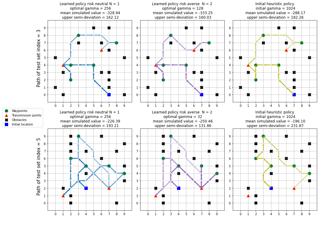
Figure 1: Robot trajectories for different policies on two random configurations (top and bottom). On the left are the trajectories of the robot using the learned risk-neutral policy. In the middle are the trajectories of the robot using the learned risk-averse policy, with the mini-batch size $N=2$. On the right are the trajectories of the robot using the initial policy of moving to the nearest relevant point (an unobserved waypoint or a transmission point). On top of each plot, we provide performance statistics obtained by multiple simulations.

6 Conclusion

A number of observations follow from the research reported here:

• Markov risk measures with mini-batch transition risk mappings lead to a tractable feature-based policy evaluation problem for which an implementable algorithm can be designed;

• It is useful to train in a high-dimensional hyperspace, involving the problem configuration;

• Stochastic methods of temporal difference learning do not work well on our test example, due to the highly random outcomes at some states;

• Policy improvement within parametric policies and with multi-step look-ahead models stabilizes the learning process;

• Risk aversion neutralizes the effect of the imperfections of feature-based models.

We believe that our observations provide a preliminary insight into risk-averse learning and control with value function approximation for Markov decision problems.

References

- [1]
- Puterman [1994] Puterman, M.L.: Markov Decision Processes. Wiley, Jersey City, NJ (1994)
- Bertsekas [2017] Bertsekas, D.P.: Dynamic Programming and Optimal Control, 4th edn. Athena Scientific, Boston (2017)
- Scandolo [2003] Scandolo, G.: Risk measures in a dynamic setting. PhD thesis, Università degli Studi di Milano, Milan, Italy (2003)
- Cheridito et al. [2006] Cheridito, P., Delbaen, F., Kupper, M.: Dynamic monetary risk measures for bounded discrete-time processes. Electronic Journal of Probability 11, 57–106 (2006)
- Ruszczyński and Shapiro [2006] Ruszczyński, A., Shapiro, A.: Conditional risk mappings. Mathematics of Operations Research 31(3), 544–561 (2006)
- Artzner et al. [2007] Artzner, P., Delbaen, F., Eber, J.-M., Heath, D., Ku, H.: Coherent multiperiod risk adjusted values and Bellman’s principle. Annals of Operations Research 152, 5–22 (2007)
- Pflug and Römisch [2007] Pflug, G.C., Römisch, W.: Modeling, Measuring and Managing Risk. World Scientific, Singapore (2007)
- Shapiro et al. [2021] Shapiro, A., Dentcheva, D., Ruszczyński, A.: Lectures on Stochastic Programming: Modeling And Theory. SIAM, Philadelphia, PA (2021)
- Ruszczyński [2010] Ruszczyński, A.: Risk-averse dynamic programming for Markov decision processes. Math. Program. 125(2, Ser. B), 235–261 (2010)
- Shen et al. [2013] Shen, Y., Stannat, W., Obermayer, K.: Risk-sensitive Markov control processes. SIAM Journal on Control and Optimization 51(5), 3652–3672 (2013)
- Lin and Marcus [2013] Lin, K., Marcus, S.I.: Dynamic programming with non-convex risk-sensitive measures. In: American Control Conference (ACC), 2013, pp. 6778–6783 (2013). IEEE
- Çavus and Ruszczyński [2014a] Çavus, O., Ruszczyński, A.: Computational methods for risk-averse undiscounted transient Markov models. Operations Research 62(2), 401–417 (2014)
- Çavus and Ruszczyński [2014b] Çavus, O., Ruszczyński, A.: Risk-averse control of undiscounted transient Markov models. SIAM Journal on Control and Optimization 52(6), 3935–3966 (2014)
- Fan and Ruszczyński [2018] Fan, J., Ruszczyński, A.: Risk measurement and risk-averse control of partially observable discrete-time Markov systems. Mathematical Methods of Operations Research 88, 161–184 (2018)
- Fan and Ruszczyński [2022] Fan, J., Ruszczyński, A.: Process-based risk measures and risk-averse control of discrete-time systems. Mathematical Programming 191, 113–140 (2022)
- Bäuerle and Glauner [2022] Bäuerle, N., Glauner, A.: Markov decision processes with recursive risk measures. European Journal of Operational Research 296(3), 953–966 (2022)
- Sutton [1988] Sutton, R.S.: Learning to predict by the methods of temporal differences. Machine Learning 3(1), 9–44 (1988)
- Bradtke and Barto [1996] Bradtke, S.J., Barto, A.G.: Linear least-squares algorithms for temporal difference learning. Machine Learning 22(1), 33–57 (1996)
- Tsitsiklis and Roy [1997] Tsitsiklis, J.N., Roy, V.: An analysis of temporal-difference learning with function approximation. IEEE Transactions on Automatic Control 42, 674–690 (1997)
- Sutton and Barto [1998] Sutton, R.S., Barto, A.G.: Reinforcement Learning: An Introduction. MIT Press, Cambridge (1998)
- Melo and Ribeiro [2007] Melo, F.S., Ribeiro, M.I.: Q-learning with linear function approximation. In: International Conference on Computational Learning Theory, pp. 308–322 (2007). Springer
- Yang and Wang [2020] Yang, Z., Wang, M.: Reinforcement learning in feature space: Matrix bandit, kernels, and regret bound. In: International Conference on Machine Learning, pp. 10746–10756 (2020). PMLR
- Jin et al. [2020] Jin, C., Yang, Z., Wang, Z., Jordan, M.I.: Provably efficient reinforcement learning with linear function approximation. In: Conference on Learning Theory, pp. 2137–2143 (2020). PMLR
- Borkar [2001] Borkar, V.S.: A sensitivity formula for risk-sensitive cost and the actor–critic algorithm. Systems & Control Letters 44(5), 339–346 (2001)
- Borkar [2002] Borkar, V.S.: Q-learning for risk-sensitive control. Mathematics of Operations Research 27(2), 294–311 (2002)
- Basu et al. [2008] Basu, A., Bhattacharyya, T., Borkar, V.S.: A learning algorithm for risk-sensitive cost. Mathematics of Operations Research 33(4), 880–898 (2008)
- Fei and Xu [2022] Fei, Y., Xu, R.: Cascaded gaps: Towards logarithmic regret for risk-sensitive reinforcement learning. In: International Conference on Machine Learning, pp. 6392–6417 (2022). PMLR
- Tamar et al. [2012] Tamar, A., Di Castro, D., Mannor, S.: Policy gradients with variance related risk criteria. In: Proceedings of the Twenty-ninth International Conference on Machine Learning, pp. 387–396 (2012)
- Prashanth and Ghavamzadeh [2014] Prashanth, L.A., Ghavamzadeh, M.: Actor-critic algorithms for risk-sensitive reinforcement learning. CoRR abs/1403.6530 (2014)
- Chow and Ghavamzadeh [2014] Chow, Y., Ghavamzadeh, M.: Algorithms for CVaR optimization in MDPs. In: Advances in Neural Information Processing Systems, pp. 3509–3517 (2014)
- Chow et al. [2017] Chow, Y., Ghavamzadeh, M., Janson, L., Pavone, M.: Risk-constrained reinforcement learning with percentile risk criteria. The Journal of Machine Learning Research 18(1), 6070–6120 (2017)
- Ma et al. [2018] Ma, W.-J., Oh, C., Liu, Y., Dentcheva, D., Zavlanos, M.M.: Risk-averse access point selection in wireless communication networks. IEEE Transactions on Control of Network Systems 6(1), 24–36 (2018)
- Yu et al. [2018] Yu, P., Haskell, W.B., Xu, H.: Approximate value iteration for risk-aware Markov decision processes. IEEE Transactions on Automatic Control 63(9), 3135–3142 (2018)
- Huang and Haskell [2017] Huang, W., Haskell, W.B.: Risk-aware Q-learning for Markov decision processes. In: 2017 IEEE 56th Annual Conference on Decision and Control (CDC), pp. 4928–4933 (2017). IEEE
- Ma et al. [2017] Ma, W.-J., Dentcheva, D., Zavlanos, M.M.: Risk-averse sensor planning using distributed policy gradient. In: 2017 American Control Conference (ACC), pp. 4839–4844 (2017). IEEE
- Tamar et al. [2014] Tamar, A., Mannor, S., Xu, H.: Scaling up robust MDPs using function approximation. In: International Conference on Machine Learning, pp. 181–189 (2014)
- Tamar et al. [2017] Tamar, A., Chow, Y., Ghavamzadeh, M., Mannor, S.: Sequential decision making with coherent risk. IEEE Transactions on Automatic Control 62(7), 3323–3338 (2017)
- Köse and Ruszczyński [2021] Köse, Ü., Ruszczyński, A.: Risk-averse learning by temporal difference methods with markov risk measures. The Journal of Machine Learning Research 22(1), 1800–1833 (2021)
- Yin et al. [2022] Yin, M., Duan, Y., Wang, M., Wang, Y.-X.: Near-optimal offline reinforcement learning with linear representation: Leveraging variance information with pessimism. In: International Conference on Learning Representation (2022)
- Lam et al. [2023] Lam, T., Verma, A., Low, B.K.H., Jaillet, P.: Risk-aware reinforcement learning with coherent risk measures and non-linear function approximation. In: The Eleventh International Conference on Learning Representations (2023)
- Cheridito and Kupper [2011] Cheridito, P., Kupper, M.: Composition of time-consistent dynamic monetary risk measures in discrete time. International Journal of Theoretical and Applied Finance 14(01), 137–162 (2011)
- Artzner et al. [1999] Artzner, P., Delbaen, F., Eber, J.-M., Heath, D.: Coherent measures of risk. Mathematical Finance 9(3), 203–228 (1999)
- Bäuerle and Ott [2011] Bäuerle, N., Ott, J.: Markov decision processes with Average-Value-at-Risk criteria. Mathematical Methods of Operations Research 74, 361–379 (2011)
- Uğurlu [2017] Uğurlu, K.: Controlled Markov decision processes with AVaR criteria for unbounded costs. Journal of Computational and Applied Mathematics 319, 24–37 (2017)
- Ding and Feinberg [2022] Ding, R., Feinberg, E.A.: Sequential optimization of CVaR. arXiv preprint arXiv:2211.07288 (2022)
- Ogryczak and Ruszczyński [1999] Ogryczak, W., Ruszczyński, A.: From stochastic dominance to mean-risk models: Semideviations as risk measures. European Journal of Operational Research 116(1), 33–50 (1999)
- Ogryczak and Ruszczyński [2002] Ogryczak, W., Ruszczyński, A.: Dual stochastic dominance and related mean-risk models. SIAM J. Optim. 13(1), 60–78 (2002)
- Rockafellar and Uryasev [2002] Rockafellar, R.T., Uryasev, S.: Conditional value-at-risk for general loss distributions. Journal of Banking & Finance 26(7), 1443–1471 (2002)
- Tsitsiklis and Van Roy [1997] Tsitsiklis, J.N., Van Roy, B.: An analysis of temporal-difference learning with function approximation. IEEE Fransactions on Automatic Control 42(5), 674–690 (1997)
- Bubeck et al. [2012] Bubeck, S., Cesa-Bianchi, N., et al.: Regret analysis of stochastic and nonstochastic multi-armed bandit problems. Foundations and Trends® in Machine Learning 5(1), 1–122 (2012)
- Lattimore and Szepesvári [2020] Lattimore, T., Szepesvári, C.: Bandit Algorithms. Cambridge University Press, Cambridge, UK (2020)
- Ayoub et al. [2020] Ayoub, A., Jia, Z., Szepesvari, C., Wang, M., Yang, L.: Model-based reinforcement learning with value-targeted regression. In: International Conference on Machine Learning, pp. 463–474 (2020). PMLR
- Modi et al. [2020] Modi, A., Jiang, N., Tewari, A., Singh, S.: Sample complexity of reinforcement learning using linearly combined model ensembles. In: International Conference on Artificial Intelligence and Statistics, pp. 2010–2020 (2020). PMLR
- Du et al. [2021] Du, S., Kakade, S., Lee, J., Lovett, S., Mahajan, G., Sun, W., Wang, R.: Bilinear classes: A structural framework for provable generalization in RL. In: International Conference on Machine Learning, pp. 2826–2836 (2021). PMLR
- Dong et al. [2019] Dong, S., Van Roy, B., Zhou, Z.: Provably efficient reinforcement learning with aggregated states. arXiv preprint arXiv:1912.06366 (2019)
- Katehakis and Smit [2012] Katehakis, M.N., Smit, L.C.: A successive lumping procedure for a class of Markov chains. Probability in the Engineering and Informational Sciences 26(4), 483–508 (2012)
- Ruszczyński and Shapiro [2006] Ruszczyński, A., Shapiro, A.: Optimization of convex risk functions. Mathematics of Operations Research 31(3), 433–452 (2006)
- Dayan [1992] Dayan, P.: The convergence of TD() for general . Machine Learning 8, 341–362 (1992)
- Peng [1993] Peng, J.: Efficient dynamic programming-based learning for control. PhD thesis, Northeastern University (1993)
- Dayan and Sejnowski [1994] Dayan, P., Sejnowski, T.: TD() converges with probability 1. Machine Learning 14, 295–301 (1994)
- Tsitsiklis [1994] Tsitsiklis, J.N.: Asynchronous stochastic approximation and Q-learning. Machine Learning 16, 185–202 (1994)
- Jaakkola et al. [1994] Jaakkola, T., Jordan, M.I., Singh, S.P.: On the convergence of stochastic iterative dynamic programming algorithms. Neural Computation 6, 1185–1201 (1994)
- Abbasi-Yadkori et al. [2011] Abbasi-Yadkori, Y., Pál, D., Szepesvári, C.: Improved algorithms for linear stochastic bandits. Advances in Neural Information Processing Systems 24, 1–19 (2011)
- Peña et al. [2009] Peña, V.H., Lai, T.L., Shao, Q.-M.: Self-Normalized Processes: Limit Theory and Statistical Applications. Springer, New York (2009)
- Glynn and Ormoneit [2002] Glynn, P.W., Ormoneit, D.: Hoeffding’s inequality for uniformly ergodic Markov chains. Statistics & Probability Letters 56(2), 143–146 (2002)
- Miasojedow [2014] Miasojedow, B.: Hoeffding’s inequalities for geometrically ergodic Markov chains on general state space. Statistics & Probability Letters 87, 115–120 (2014)
- Moulos [2020] Moulos, V.: A Hoeffding inequality for finite state Markov chains and its applications to Markovian bandits. In: 2020 IEEE International Symposium on Information Theory (ISIT), pp. 2777–2782 (2020). IEEE
- Jünger et al. [1995] Jünger, M., Reinelt, G., Rinaldi, G.: The traveling salesman problem. Handbooks in Operations Research and Management Science 7, 225–330 (1995)
- Cook et al. [2011] Cook, W.J., Applegate, D.L., Bixby, R.E., Chvatal, V.: The Traveling Salesman Problem: a Computational Study. Princeton University Press, Princeton, NJ (2011)