Privacy Preserving Event Detection

Abstract

This paper presents a privacy-preserving event detection scheme based on measurements made by a network of sensors. A diameter-like decision statistic made up of the marginal types of the measurements observed by the sensors is employed. The proposed detection scheme can achieve the best type-I error exponent as the type-II error rate is required to be negligible. Detection performance with finite-length observations is also demonstrated through a simulation example of spectrum sensing. Privacy protection is achieved by obfuscating the type data with random zero-modulo-sum numbers that are generated and distributed via the exchange of encrypted messages among the sensors. The privacy-preserving performance against “honest but curious” adversaries, including colluding sensors, the fusion center, and external eavesdroppers, is analyzed through a series of cryptographic games. It is shown that the probability that any probabilistic polynomial time adversary successfully estimates the sensors’ measured types can not be much better than independent guessing, when there are at least two non-colluding sensors.

I Introduction

A typical event detection system consists of a network of sensors distributed in a target area for collecting and reporting measurement data to a fusion center which aggregates the reported data to make a detection decision. In this paper, we develop a privacy-preserving event detection scheme, in which the sensors obfuscate the square roots of the marginal types (empirical distributions) of their measurements with random zero-modulo-sum (ZMS) numbers before uploading them to the fusion center, which then performs a binary hypothesis test based on a diameter-like statistic that measures the scattering level of the uploaded types. In this way, the target event can be detected without exposing the data of individual sensors.

Our scheme consists of two interconnected parts. One is a test that focuses on achieving the best error exponents in the hypothesis test, and the other is a privacy-preserving protocol that focuses on minimizing the probability of potential attackers successfully estimating the sensors’ types. A distinguishing feature of the proposed test is that the decision statistic is an aggregation of distributed components that can be computed at each sensor individually. Hence, only these components, rather than the raw observations, are required to be sent to the fusion center. Privacy protection thus needs to apply to only these components. This decentralized property is critical in making the simple ZMS privacy-preserving protocol work. In all, our objective is to show that a joint detection-privacy design can provide good detection performance as well as a verifiable privacy guarantee using only a simple privacy-preserving scheme.

I-A The $K$-sample problem

Crowd-sensing of spectrum occupancy in, e.g., the citizen broadband radio service (CBRS) band by smart phones (see Section IV-C for a more detailed example) is a practical application that motivates the event detection problem considered. Intuitively, the distributions of the received powers measured by distributed sensors would be different when a potential source is transmitting because of the different distances between the source and the sensors. On the other hand, when the source is silent, the received power distributions would be similar because only noise is present in the sensors’ received signals. Thus, comparing the similarity of the power distributions across the sensors would allow us to determine whether the source is transmitting or not, without any a priori information of the sensors’ power distributions.

This simple intuitive approach is effectively an extension to the classical $K$-sample problem, which is to test whether the multiple samples are drawn from the same unspecified distribution. During the past decades, a variety of tests have been proposed to solve this problem. Many of these tests, such as the Kruskal-Wallis test [1], Terry-Hoeffding test [2], rank tests against the ordered alternatives [3] and the named umbrella alternatives [4], extended Anderson-Darling tests [5], and modified Baumgartner test [6], are based on ranking the observations from all samples (sensors). The ranking operation requires the sensors to report all their observations to the fusion center for calculating the decision statistic. As a result, privacy protection would be required for the raw data of all sensors. Some non-ranking tests, such as the extended one-way analysis of variance F-test [7] and $e$-distance based energy test [8], also have the same requirement of the raw sensor observations be available at the fusion center, and hence require complicated privacy protection mechanism. The decision statistics of the $K$-sample Kolmogorov-Smirnov and Cramér-von Mises tests [9] and empirical Bayes factor test based on the Polya tree priors [10], on the other hand, can be expressed as functions of distributed components that can be calculated at the sensors. Nonetheless, these functions have complicated forms, which may require multiple rounds of obfuscation to protect the privacy of the distributed components. In general, the detection performance of all the above tests is analyzed based on the limiting and/or approximate distributions of the statistics, and is verified through the simulations with artificial or real world data sets (see [8]).

The extension to the basic $K$-sample problem considered here is that the marginal distributions of the sensors’ observations do not need to be exactly the same under the null hypothesis. We formulate this extended $K$-sample problem and study the best achievable error exponents in Section III. In the same section, we propose a test in which the fusion center only needs the sensors to report the square roots of the marginal types of their measurement data in order to compute a statistic that is the sum of the Hellinger distance squares between all pair of marginal types. We show that the proposed test is optimal in a sense that the best type-I error exponent can be achieved while requiring the type-II error to be negligible. This result is further illustrated in Section IV-C by a simulation example of a spectrum sensing scenario employing the CBRS channel model. A disadvantage of the proposed test is that more observations are often needed, compared to some of the other tests described before, because of the use of marginal types in the decision statistic. This is nonetheless a minor issue for the considered crowd-sensing scenario in which an abundent number of observations are usually available at each sensor.

I-B Privacy protection

In many applications, it is desirable to protect the sensors’ data and/or statistics reported to the fusion center as they may expose private information about the sensors themselves. A number of mechanisms have been proposed to provide some form of privacy protection.

An intuitive approach is to homomorphically encrypt the measurement data and have the message transmission, statistic computation, and event detection all conducted in the ciphertext domain. For example, ref. [11] designs a received-signal-strength fingerprinting localization scheme called PriWFL by leveraging the Paillier cryptosystem to preserve location privacy of users and data privacy of the service provider. The PriWFL scheme is extended in [12] to support channel state information fingerprinting localization and to give further protection on position privacy of the localization infrastructure. The main drawback of homomorphic encryption is its high computational overheads. As mentioned before, the decentralized property of our proposed test allows us to avoid using homomorphic encryption to achieve privacy protection.

Another approach is based on compressive sensing (CS). Pseudo-random measurement matrices are employed to linearly encode the sensors’ measurements, which are then recovered at the fusion center. Based on this approach, a privacy-preserving federated learning (FL) scheme for spectrum detection in CBRS is proposed in [13], and a multi-level privacy-preserving scheme for the users with different privilege levels to acquire and analyze the data is constructed in [14]. A critical issue of the CS approach is how to generate and distribute the secret measurement matrices. In the above examples, the required secrecy is generated from channel reciprocity between wireless transceivers [13] and from a chaotic system [14]. It is however difficult to obtain verifiable secrecy from both of these mechanisms. In contrast, by leveraging standard public-key encryption, our proposed privacy-preserving scheme provides verifiable protection to the sensors’ statistics.

Another large category of privacy-preserving techniques involves perturbing the sensors’ original data with well designed noise such that the perturbed data can still yield an acceptable level of performance. A popular design methodology of perturbation is based on differential privacy (DP) [15], which aims to constrain the distance between any pair of outputs provided the input collections only differ in one data point. Under the DP constraint, ref. [16] develops a FL scheme called NbAFL, which lets the fusion center perturb the global model in the downlink transmission and the users perturb the local models in the uplink transmission. In [17], FL is implemented under the DP constraint over a Gaussian multiple access channel to extract privacy benefit from the underlying physical layer characteristics. The main shortcoming of perturbation is the inevitable performance degradation caused by the introduced noise. In addition, when the number of sensors and the dimension of data are large, the DP guarantee may not be practically sufficient. More importantly, the DP guarantee is derived from a defender’s perspective rather than against the objective and/or capability of a potential attacker. On the contrary, our privacy-preserving design directly considers the attacker’s probability of the successful estimation of the sensors’ measured types.

I-C Zero-modulo-sum obfuscation

The decentralized property and the additive nature of the proposed decision statistic allow us to employ a classical ZMS obfuscation scheme to protect the sensors’ data privacy. Specifically, each sensor generates a collection of uniform ZMS random numbers, among which one number is kept secret to the sensor itself, and other numbers are confidentially sent to other sensors by way of a public key cryptosystem. Then, each sensor obfuscates its measured square-root type by calculating the modulo sum of the type, the self-kept number and the received numbers such that all the obfuscation can be eventually canceled out at the fusion center. The detailed protocol to apply this ZMS obfuscation scheme is discussed in Section IV.

In Section V, we analytically quantify the privacy protection performance of the ZMS obfuscation scheme under an “honest but curious” threat model in which the adversary may include external eavesdroppers, the fusion center, and a subset of sensors all colluding to estimate the other sensors’ measured types. We apply the standard attacker-challenger formalism in cryptographic analysis to show that any probabilistic polynomial time (PPT) attacker can not improve the probability of correctly estimating the sensors’ measured types beyond independent guessing given the information that she can obtain from her own measurement and that is “leaked” to her via the proposed protocol, provided that the public key cryptosystem to used distribute the ZMS random numbers is secure under the chosen plaintext attack (CPA) criterion.

ZMS obfuscation is widely used in many different applications. We highlight here some related recent works. A zero-sum (but not modulo sum) obfuscating mechanism is adopted in [18] as an intermediate step to achieve privacy-preserving localization. Ref. [19] applies ZMS obfuscation to perform data aggregation in wireless sensor networks, where the data are obfuscated in a closed-loop order through all sensors. Similarly, ZMS obfuscation is applied in [20] to a smart grid, where data aggregation is conducted with the help of hash functions. In [21], the protocols of secret sharing and multi-party anonymous authentication are developed with ZMS obfuscation, and the detection of dishonest participants is discussed. Another related work is [22], in which a secure aggregation protocol, called SecAgg, is proposed for FL. The protocol utilizes random numbers generated by pseudo random generators (PRGs) to obfuscate model updates from the FL participants. The seeds of PRGs are negotiated via a Diffie-Hellman exchange between each participant pair, including any malicious participants. The privacy analysis of [21] and [22] is performed based on an abstract concept called view, which encapsulates the information that can be obtained from the set of inputs available to an adversary.

In regard to the above works, the main contribution of the analysis presented in Section V is that we are able to quantify the level of privacy protection provided by the proposed scheme in terms of the direct and concrete privacy metric of successful estimation probability by any PPT attacker, while allowing any colluding sensors to adaptively generate their ZMS numbers based on all the messages that they have received.

II Notation and Assumptions

II-A Basic Notation

We use uppercase letters and the corresponding lowercase letters to denote random variables and the values taken by the random variables, respectively. We use boldface letters to denote an indexed collection of random variables and values. Script letters are generally reserved for index sets and alphabets. When an index set is employed as a subscript, we refer to the collection of random variables (or values) indexed over the set. For convenience, we slightly abuse notation by using a single index to also denote a singleton index set containing only that index. For example, given a sensor network with $K$ sensors, $\mathcal{K}=\{1,2,\ldots,K\}$ denotes the set of sensor indices, $\mathcal{X}$ denotes the finite alphabet of sensor measurements, $\mathbf{X}_{k}=[X_{k,i}]_{i=1}^{t}\in\mathcal{X}^{t}$ denotes the $t$-length measurement sequence of the $k$th sensor, and $\mathbf{X}_{\mathcal{K}}=[\mathbf{X}_{k}]_{k\in\mathcal{K}}\in\mathcal{X}^{Kt}$ denote the collection of measurement sequences from all sensors.

For the rest of the paper, we assume the sensor measurement alphabet $\mathcal{X}$ is finite with $\mathcal{P}(\mathcal{X})$ denoting the set of distributions (probability mass functions) over $\mathcal{X}$. The distribution of a random variable $X$ over $\mathcal{X}$ is denoted by $p_{X}$. When convenient, we may write a distribution $p\in\mathcal{P}(\mathcal{X})$ as a vector, i.e., $\mathbf{p}=[p(x)]_{x\in\mathcal{X}}$. For any $t$-length measurement sequence $\mathbf{X}_{k}$, $\tilde{q}_{\mathbf{X}_{k}}(x)=\frac{1}{t}\cdot\left(\text{number of occurrences of~{}}x\text{~{}in~{}}\mathbf{X}_{k}\right)$ denotes the type (empirical distribution) of $\mathbf{X}_{k}$. The set of all possible types of $t$-length sequences is denoted by $\tilde{\mathcal{Q}}_{t}(\mathcal{X})$. Note that $\bigcup_{t=1}^{\infty}\tilde{\mathcal{Q}}_{t}(\mathcal{X})$ is dense in $\mathcal{P}(\mathcal{X})$. Furthermore, for any $\tilde{q}\in\tilde{\mathcal{Q}}_{t}(\mathcal{X})$, we denote its type class by $\mathcal{T}(\tilde{q})=\{\mathbf{x}\in\mathcal{X}^{t}:\tilde{q}_{\mathbf{x}}=\tilde{q}\}$.

A vector of $K$ marginal distributions is denoted by $\mathbf{p}_{\mathcal{K}}=[p_{k}]_{k\in\mathcal{K}}\in\mathcal{P}^{K}(\mathcal{X})$, with each $p_{k}\in\mathcal{P}(\mathcal{X})$. With a slight abuse of notation, we also use the same notation $\mathbf{p}_{\mathcal{K}}$ to denote a general joint distribution in $\mathcal{P}(\mathcal{X^{K}})$. When necessary to highlight the former case, we will explicitly state $\mathbf{p}_{\mathcal{K}}\in\mathcal{P}^{K}(\mathcal{X})$. The same convention applies to vectors of marginal types in $\tilde{\mathcal{Q}}_{t}^{K}(\mathcal{X})$ and joint types in $\tilde{\mathcal{Q}}_{t}(\mathcal{X}^{K})$.

For any $p_{k},p_{l}\in\mathcal{P}(\mathcal{X})$, the Hellinger distance square between them [23] is given by

$$d^{2}_{H}(p_{k},p_{l}) =\frac{1}{2}\sum_{x\in\mathcal{X}}\left(\sqrt{{p}_{k}(x)}-\sqrt{{p}_{l}(x)}\right)^{2}.$$

Definition 1.

For any $\mathbf{p}_{\mathcal{K}}\in\mathcal{P}^{K}(\mathcal{X})$, define its “diameter” to be

$$d(\mathbf{p}_{\mathcal{K}}) =\sum_{k\in\mathcal{K}}\sum_{l\in\mathcal{K}}d^{2}_{H}(p_{k},p_{l})=K^{2}-\sum_{x\in\mathcal{X}}\left(\sum_{k=1}^{K}\sqrt{{p}_{k}(x)}\right)^{2}.$$ (1)

This definition naturally extends to any general $\mathbf{p}_{\mathcal{K}}\in\mathcal{P}(\mathcal{X}^{K})$ in that the $p_{k}$’s in (1) are taken as the corresponding marginals of $\mathbf{p}_{\mathcal{K}}$. Let

$$d_{\max}= K(K-1)-\left\lfloor\frac{K}{|\mathcal{X}|}\right\rfloor(K-|\mathcal{X}|+K\bmod|\mathcal{X}|).$$ (2)

Then, it is not hard to show that $0\leq d(\mathbf{p}_{\mathcal{K}})\leq d_{\max}$ for any $\mathbf{p}_{\mathcal{K}}\in\mathcal{P}(\mathcal{X}^{K})$.

For each $x_{0}\in\mathcal{X}$, the indicator function $\delta_{x_{0}}(x)=1$ if $x=x_{0}$, and $\delta_{x_{0}}(x)=0$ otherwise. This defintion naturally extends when the arguments are collections. Any other function $F(X)$ in this paper, under otherwise stated, is assumed stochastic. That is, $F(X)$ is random and is conditionally independent of all other random variables given its input $X$.

II-B Fixed-point Arithmetics

Let $N$ be a positive integer and $\mathcal{N}_{m}$ be the collection of all $m$-bit fixed-point numbers quantizing the interval $[0,N)$, i.e., $\mathcal{N}_{m}=\left\{0,\frac{N}{2^{m}},\ldots,\frac{(2^{m}-1)N}{2^{m}}\right\}$. We “quantize” each $\tilde{q}\in\mathcal{\tilde{Q}}_{t}(\mathcal{X})$ by mapping $\sqrt{\tilde{q}(x)}$, for each $x\in\mathcal{X}$, to its closest value in $\mathcal{N}_{m}$. Let $\mathcal{Q}_{t}(\mathcal{X})$ denote the set of quantized (to $\mathcal{N}_{m}$) square roots of the types in $\mathcal{\tilde{Q}}_{t}(\mathcal{X})$. More specifically, every $\tilde{q}\in\mathcal{\tilde{Q}}_{t}(\mathcal{X})$ is mapped to a $q\in\mathcal{Q}_{t}(\mathcal{X})$ that satisfies $q(x)\in\mathcal{N}_{m}$, $0\leq q(x)\leq 1$, and $|\sqrt{\tilde{q}(x)}-q(x)|\leq 2^{-m-1}$ for every $x\in\mathcal{X}$. Note that $q^{2}$ may not be a true type; however it must satisfy $\left|\sum_{x\in\mathcal{X}}q^{2}(x)-1\right|\leq 2^{-m}|\mathcal{X}|$. We assume that $m$ is chosen large enough to guarantee $q^{2}$ is sufficiently close to a true type. We also note that $|\mathcal{Q}_{t}(\mathcal{X})|\leq|\mathcal{\tilde{Q}}_{t}(\mathcal{X})|\leq(t+1)^{|\mathcal{X}|}$ [24, Theorem 11.1.1]. With a large enough $m$ (i.e., $m=\mathcal{O}(\log_{2}t)$), we assume $|\mathcal{Q}_{t}(\mathcal{X})|$ to have the same order as $|\mathcal{\tilde{Q}}_{t}(\mathcal{X})|$.

Let $\oplus$ and $\ominus$ denote addition and subtraction modulo $N$ over the fixed-point numbers in $\mathcal{N}_{m}$, respectively. Note that $\mathcal{N}_{m}$ is closed under both the operations. If the operands of $\oplus$ or $\ominus$ are indexed collections, it means performing the $\oplus$ or $\ominus$ operation elementwise. For any $x_{0}\in\mathcal{N}_{m}$, the indicator function $\delta_{x_{0}}(x)=\delta_{0}(x\ominus x_{0})$ for all $x\in\mathcal{N}_{m}$. We will omit the subscript $0$ in $\delta_{0}$ and write $\delta(x\ominus x_{0})$ as the indicator function.

For a collection of random variables $[Y_{k}(x)]$ on $\mathcal{N}_{m}$, indexed by $k\in\mathcal{K}$ and $x\in\mathcal{X}$, we write $\mathbf{Y}_{\mathcal{L}}(x)=[Y_{k}(x)]_{k\in\mathcal{L}}$ and $\mathbf{Y}_{\mathcal{L}}=[\mathbf{Y}_{\mathcal{L}}(x)]_{x\in\mathcal{X}}$ for any $\mathcal{L}\subseteq\mathcal{K}$. We use the notation $\mathbf{Y}_{\mathcal{K}}\sim{u}(\mathcal{N}^{K|\mathcal{X}|}_{m})$ to say $\mathbf{Y}_{\mathcal{K}}$ is uniformly distributed on $\mathcal{N}^{K|\mathcal{X}|}_{m}$, i.e., all elements in $\mathbf{Y}_{\mathcal{K}}$ are independent and identically distributed (i.i.d.) according to ${u}(\mathcal{N}_{m})$.

Similarly for a collection of random variables $[R_{k,l}(x)]$ on $\mathcal{N}_{m}$, indexed by $(k,l)\in\mathcal{K}^{2}$ and $x\in\mathcal{X}$, we write $\mathbf{R}_{\mathcal{I},\mathcal{J}}(x)=[R_{k,l}(x)]_{k\in\mathcal{I},l\in\mathcal{J}}$ and $\mathbf{R}_{\mathcal{I},\mathcal{J}}=[\mathbf{R}_{\mathcal{I},\mathcal{J}}(x)]_{x\in\mathcal{X}}$ for any $\mathcal{I},\mathcal{J}\subseteq\mathcal{K}$. In addition, we define $\mathbf{\Sigma}_{\mathbf{Y}_{\mathcal{L}}}(x)=\bigoplus_{k\in\mathcal{L}}Y_{k}(x)$, $\mathbf{\Sigma}_{\mathbf{Y}_{\mathcal{L}}}=[\Sigma_{\mathbf{Y}_{\mathcal{L}}}(x)]_{x\in\mathcal{X}}$, $\mathbf{\Sigma}_{\mathbf{R}_{\mathcal{I},\mathcal{J}}}(x)=[\bigoplus_{i\in\mathcal{I}}R_{k,l}(x)]_{l\in\mathcal{J}}$, and $\mathbf{\Sigma}_{\mathbf{R}_{\mathcal{I},\mathcal{J}}}=[\mathbf{\Sigma}_{\mathbf{R}_{\mathcal{I},\mathcal{J}}}(x)]_{x\in\mathcal{X}}$.

II-C Cryptographic Assumptions

We review here some standard cryptographic concepts and assumptions useful for constructing and analyzing our privacy preserving mechanism in later sections. In particular, we will follow the standard cryptographic methodology that defines an attack experiment involving two interactive parties, namely a challenger and an attacker, and evaluates the probability advantage of the attacker winning the experiment. To that end, the attack experiments will be based on the well known chosen-plaintext attack (CPA) model [25].

Consider

• a public-key cryptographic scheme $\Pi=(S,E,D)$ with security parameter $n$, and

• a probabilistic, polynomial-time (PPT) attacker, whose running time is polynomial in $n$.

The functions $S$, $E$, and $D$ represent the algorithms of key generation, encryption, and decryption, respectively. The security parameter $n$ is usually formulated in the unary form as $1^{n}$, a string of $n$ $1$’s. In this paper, we restrict each plaintext in $\Pi$ to be an $m$-bit message corresponding to a fixed-point number in $\mathcal{N}_{m}$, and the resulting ciphertext space is denoted by $\mathcal{C}$. As shown in Figure 1, the CPA experiment is defined as follows:

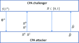
Figure 1: The CPA experiment.

1. The challenger runs $S(1^{n})$ to generate a pair of public key $\Phi^{n}\in\mathcal{E}_{n}$ and private key $\Psi^{n}\in\mathcal{D}_{n}$, and then gives $\Phi^{n}$ to the attacker. This means that attacker can encrypt any plaintext by executing $E(\cdot;\Phi^{n})$ herself.

2. The attacker generates a pair of challenge messages $[R^{0},R^{1}]\sim{u}(\mathcal{N}^{2}_{m})$, and gives them to her challenger.

3. The challenger selects an independent random bit $B\in\{0,1\}$ with equal probabilities, computes the ciphertext $C^{B}=E(R^{B};\Phi^{n})\in\mathcal{C}$, and gives $C^{B}$ to the attacker.

4. The attacker outputs a bit $\hat{B}=\hat{B}(C^{B},R^{0},R^{1},\Phi^{n})$ as her estimate of $B$. Then, she reports $\hat{B}$ to her challenger.

If $\hat{B}=B$, it is said that the attacker wins the CPA experiment. Define the probability advantage of the attacker winning the CPA experiment as

$$F_{\mathrm{CPA}}(n)=\Pr(\hat{B}=B)-\frac{1}{2}.$$ (3)

Based on the CPA experiment described above, we define the CPA security of a public key scheme as follows [25]:

Definition 2.

A public key encryption scheme $\Pi=(S,E,D)$ is said to be CPA-secure if there exists a negligible function $\varepsilon(n)$ such that $F_{\mathrm{CPA}}(n)\leq\varepsilon(n)$ for all PPT attackers.

Note that many practical public-key cryptographic schemes, such as ElGamal [26] and RSA-OAEP [27], have been shown to be CPA-secure.

For the rest of this paper, we make the following assumptions on the cryptographic resources available to the sensors.

Assumption 3.

(Cryptographic resource) The same CPA-secure public-key cryptographic scheme $\Pi=(S,E,D)$ with security parameter $n$ is made available to each sensor, that maintains its own pair of public and private keys. The public keys for encrypting messages are known to all entities in the network while the private keys for decrypting messages are secret.

Assumption 4.

(Independent Encryptions) Every use of the encryption function is conditionally independent of all other uses given the plaintexts and public keys. More precisely, let $M$ be any positive integer and $C_{k}={E}(R_{k};\Phi_{k}^{n})$ for $k=1,2,\ldots,M$. Then for any $c_{k}\in\mathcal{C}$, $r_{k}\in\mathcal{N}_{m}$, and $\phi_{k}\in\mathcal{E}_{n}$,

$$p_{C_{1},\ldots,C_{M}\mid R_{1},\ldots,R_{M},\Phi_{1}^{n},\ldots,\Phi_{M}^{n}}(c_{1},\ldots,c_{M}\mid r_{1},\ldots,r_{M},\hskip 30.0pt$$

$$\phi_{1}^{n},\ldots,\phi_{M}^{n})=\prod_{k=1}^{M}p_{C_{k}\mid R_{k},\Phi_{k}^{n}}(c_{k}\mid r_{k},\phi_{k}^{n}).$$

Furthermore, we adopt the following “bar” notation to simplify discussion in later sections. For any $\mathcal{I},\mathcal{J}\subseteq\mathcal{K}$ and a collection of plaintexts $\mathbf{R}_{\mathcal{I},\mathcal{J}}=[R_{k,l}(x)]_{k\in\mathcal{I},l\in\mathcal{J},x\in\mathcal{X}}$, the corresponding “barred” collection is defined as ${\mathbf{\bar{R}}}_{\mathcal{I},\mathcal{J}}=[R_{k,l}(x)]_{k\in\mathcal{I},l\in\mathcal{J}\setminus k,x\in\mathcal{X}}$. Given a collection of public keys $\mathbf{\Phi}_{\mathcal{J}}^{n}=[\Phi_{l}^{n}]_{l\in\mathcal{J}}$ with $\Phi_{l}^{n}\in\mathcal{E}_{n}$, we write ${\mathbf{\bar{C}}}_{\mathcal{I},\mathcal{J}}=E(\mathbf{\bar{R}}_{\mathcal{I},\mathcal{J}};\mathbf{\Phi}_{\mathcal{J}}^{n})$ as a shorthand for the operations of computing the ciphertext $C_{k,l}(x)=E(R_{k,l}(x);\Phi_{l}^{n})$ for each $k\in\mathcal{I}$, $l\in\mathcal{J}\setminus k$, $x\in\mathcal{X}$, and outputting the whole ciphertext collection $\mathbf{\bar{C}}_{\mathcal{I},\mathcal{J}}=[C_{k,l}(x)]_{k\in\mathcal{I},l\in\mathcal{J}\setminus k,x\in\mathcal{X}}$. Similarly, given a collection of private keys $\mathbf{\Psi}_{\mathcal{J}}^{n}=[\Psi_{l}^{n}]_{l\in\mathcal{J}}$ with $\Psi_{l}^{n}\in\mathcal{D}_{n}$, we write ${\mathbf{\bar{R}}}_{\mathcal{I},\mathcal{J}}=D(\bar{\mathbf{C}}_{\mathcal{I},\mathcal{J}};\mathbf{\Psi}^{n}_{\mathcal{J}})$ as a shorthand for the operations of computing the plaintext $R_{k,l}(x)=D(C_{k,l}(x);\Psi_{l}^{n})$ for each $k\in\mathcal{I}$, $l\in\mathcal{J}\setminus k$, $x\in\mathcal{X}$, and outputting the whole plaintext collection ${\mathbf{\bar{R}}}_{\mathcal{I},\mathcal{J}}=[R_{k,l}(x)]_{k\in\mathcal{I},l\in\mathcal{J}\setminus k,x\in\mathcal{X}}$. It is obvious that if $\mathcal{I}\cap\mathcal{J}=\emptyset$, then $\mathbf{R}_{\mathcal{I},\mathcal{J}}={\mathbf{\bar{R}}}_{\mathcal{I},\mathcal{J}}$ and $\mathbf{C}_{\mathcal{I},\mathcal{J}}={\mathbf{\bar{C}}}_{\mathcal{I},\mathcal{J}}$.

III Event Detection

In this section, we introduce the formulation of the event detection problem, propose a detector that facilitates privacy protection, and analyze the error exponents achieved by the proposed detector.

III-A Problem Formulation

As mentioned before, we consider a network of $K$ sensors together with a fusion center that aggregates information from the sensors to perform detection of a target event. The network size $K$ is assumed to be fixed and known to all entities in the sensor network. Communications between the fusion center and the sensors are assumed public. All messages sent by any entity are observable by all entities within and outside of the network. Moreover, all entities agree on a positive number $N>K$, a large enough integer $m$, and thus the resulting fixed-point domain $\mathcal{N}_{m}$ beforehand.

Let $\mathbf{X}_{k}$ be a $t$-length measurement vector made by the $k$th sensor, for $k\in\mathcal{K}=\{1,2,\ldots,K\}$. The elements of $\mathbf{X}_{k}$ are i.i.d. according to the marginal distribution $p_{\theta,k}$ over the common finite alphabet $\mathcal{X}$. The parameter $\theta\in\{0,1\}$ represents the system state indicating whether the target event happens ($\theta=1$) or not ($\theta=0$). The distributions $p_{0,k}$ and $p_{1,k}$ may contain private information about the $k$th sensor. For convenience, we write the distributions as vectors: $\mathbf{p}_{0,k}=[p_{0,k}(x)]_{x\in\mathcal{X}}$ and $\mathbf{p}_{1,k}=[p_{1,k}(x)]_{x\in\mathcal{X}}$, and consider the joint distributions $\mathbf{p}_{0,\mathcal{K}}\in\mathcal{P}(\mathcal{X}^{K})$ and $\mathbf{p}_{1,\mathcal{K}}\in\mathcal{P}(\mathcal{X}^{K})$, whose marginals are respectively given by $[\mathbf{p}_{0,k}]_{k\in\mathcal{K}}$ and $[\mathbf{p}_{1,k}]_{k\in\mathcal{K}}$. We assume that neither $\mathbf{p}_{0,\mathcal{K}}$ nor $\mathbf{p}_{1,\mathcal{K}}$ is known. However, it is known that they satisfy the condition

$$d\left(\mathbf{p}_{0,\mathcal{K}}\right)\leq d_{0}<d_{1}\leq d\left(\mathbf{p}_{1,\mathcal{K}}\right)$$ (4)

for some $0\leq d_{0}<d_{1}\leq d_{\max}$.

The objective of the fusion center is to make a decision on the system state $\theta$ based on the whole set of sensor measurements $\mathbf{X}_{\mathcal{K}}\in\mathcal{X}^{Kt}$. In this section, we temporarily ignore any privacy concern and assume that any necessary statistics (e.g., $\mathbf{X}_{\mathcal{K}}$) for decision are made available to the fusion center. In Section IV, we will present a protocol to protect privacy specifically for the application of the following binary hypothesis test at the fusion center to make a decision on $\theta$: The $k$th sensor calculates the type $\tilde{Q}_{k}=\tilde{q}_{\mathbf{X}_{k}}$ from its measurement sequence $\mathbf{X}_{k}$, and sends $\tilde{Q}_{k}$ to the fusion center. The fusion center collects the whole set of sensor types $\mathbf{\tilde{Q}}_{\mathcal{K}}\in\tilde{\mathcal{Q}}_{t}^{K}(\mathcal{X})$ from the $K$ sensors, calculate the diameter of $\mathbf{\tilde{Q}}_{\mathcal{K}}$, and then decides

$$H_{0} :\theta=0\quad\quad\text{if}\ d({\mathbf{\tilde{Q}}}_{\mathcal{K}})<\gamma$$ (5)

$$H_{1} :\theta=1\quad\quad\text{if}\ d({\mathbf{\tilde{Q}}}_{\mathcal{K}})\geq\gamma$$

where $\gamma\geq 0$ is a detection threshold. Note that the decision statistic $d({\mathbf{\tilde{Q}}}_{\mathcal{K}})$ employed in the test above depends only on the marginal types $[\tilde{Q}_{k}]_{k\in\mathcal{K}}$, each of which can be calculated at the corresponding sensor based on its own measurement vector.

III-B Error Exponents

In this section, we analyze the detection performance of the binary test (5). To that end, define the following two sets of joint distributions:

$$\mathcal{P}_{0,\mathcal{K}} =\{\mathbf{p}_{\mathcal{K}}\in\mathcal{P}(\mathcal{X}^{K}):d(\mathbf{p}_{\mathcal{K}})\leq d_{0}\}$$

$$\mathcal{P}_{1,\mathcal{K}} =\{\mathbf{p}_{\mathcal{K}}\in\mathcal{P}(\mathcal{X}^{K}):d(\mathbf{p}_{\mathcal{K}})\geq d_{1}\}.$$

For a binary hypothesis test with acceptance region $\mathcal{R}_{t}\subseteq\mathcal{X}^{Kt}$, we define the (worst-case) error probability of the first type as

$$\mu_{t}=\max_{\mathbf{p}_{0,\mathcal{K}}\in\mathcal{P}_{0,\mathcal{K}}}\mathbf{p}_{0,\mathcal{K}}(\mathcal{R}_{t}^{c})$$ (6)

and the (worst-case) error probability of the second type as

$$\lambda_{t}=\max_{\mathbf{p}_{1,\mathcal{K}}\in\mathcal{P}_{1,\mathcal{K}}}\mathbf{p}_{1,\mathcal{K}}(\mathcal{R}_{t}).$$ (7)

Based on these error probabilities, we define an achievable error exponent pair as follows:

Definition 5.

A non-negative error exponent pair $(\alpha,\beta)$ is said to be achievable if there is a sequence of acceptance regions such that

$$\liminf_{t\rightarrow\infty}-\frac{1}{t}\log_{2}\mu_{t} \geq\alpha$$ (8)

$$\liminf_{t\rightarrow\infty}-\frac{1}{t}\log_{2}\lambda_{t} \geq\beta.$$ (9)

A non-negative error exponent of the first type $\alpha$ is said to be achievable if there is a sequence of acceptance regions such that (8) is satisfied and $\lim_{t\rightarrow\infty}\lambda_{t}=0$.

Clearly, if $(\alpha,\beta)$ is achievable and $\beta>0$, then $\alpha$ is achievable. Thus, $(\alpha,\beta)$ being an achievable error exponent pair is a stronger condition.

For $\mathbf{p}_{\mathcal{K}}\in\mathcal{P}(\mathcal{X}^{K})$, define

$$\Delta_{0}(\mathbf{p}_{\mathcal{K}}) =\min_{\mathbf{p}_{0,\mathcal{K}}\in\mathcal{P}_{0,\mathcal{K}}}D(\mathbf{p}_{\mathcal{K}}\|\mathbf{p}_{0,\mathcal{K}})$$

$$\Delta_{1}(\mathbf{p}_{\mathcal{K}}) =\min_{\mathbf{p}_{1,\mathcal{K}}\in\mathcal{P}_{1,\mathcal{K}}}D(\mathbf{p}_{\mathcal{K}}\|\mathbf{p}_{1,\mathcal{K}})$$

where $D(\cdot\|\cdot)$ is the Kullback-Leibler (KL) divergence. For $\gamma\geq 0$, define the function

$$\alpha_{*}(\gamma)=\min_{\mathbf{p}_{\mathcal{K}}\in\mathcal{P}(\mathcal{X}^{K}):d(\mathbf{p}_{\mathcal{K}})\geq\gamma}\Delta_{0}(\mathbf{p}_{\mathcal{K}}).$$

Further, for $\alpha\geq 0$, define

$$\gamma_{*}(\alpha) =\inf\{\gamma\geq 0:\alpha_{*}(\gamma)\geq\alpha\},$$

$$\beta_{*}(\alpha) =\inf_{\mathbf{p}_{\mathcal{K}}\in\mathcal{P}(\mathcal{X}^{K}):d(\mathbf{p}_{\mathcal{K}})<\gamma_{*}(\alpha)}\Delta_{1}(\mathbf{p}_{\mathcal{K}}),$$

$$\beta^{*}(\alpha) =\inf_{\mathbf{p}_{\mathcal{K}}\in\mathcal{P}(\mathcal{X}^{K}):\Delta_{0}(\mathbf{p}_{\mathcal{K}})<\alpha}\Delta_{1}(\mathbf{p}_{\mathcal{K}}).$$

The following theorem expresses the best error exponent and best error exponent pair of the event detection problem in terms of the functions defined above:

Theorem 6.

Suppose $0\leq d_{0}<d_{1}\leq d_{\max}$. Then

1. $\beta_{*}(\alpha)\leq\beta^{*}(\alpha)$,

2. $\beta^{*}(\alpha)>0$ if and only if $\beta_{*}(\alpha)>0$,

3. $\beta^{*}(\alpha)=\sup\{\beta:(\alpha,\beta)\text{~{}is achievable}\}$,

4. $\alpha_{*}(d_{1})=\sup\{\alpha:\alpha\text{~{}is achievable}\}$, and

5. the test (5) achieves the error exponent pair $(\alpha,\beta_{*}(\alpha))$ and the supremum error exponent $\alpha_{*}(d_{1})$.

Proof.

The proof of the theorem is given in Appendix A. While the test (5) may not achieve the best error exponent pair $(\alpha,\beta^{*}(\alpha))$, it is able to achieve a positive error exponent pair whenever the best test can. The test (5) nevertheless is optimal in the weaker sense that it can achieve the best error exponent of the first kind. In either case, it suffices to choose the decision threshold $\gamma\in(d_{0},d_{1})$.

As shown in the proof of part (iii) in Appendix A, a test using the decision statistic $\Delta_{0}({\mathbf{\tilde{Q}}}_{\mathcal{K}})$, where ${\mathbf{\tilde{Q}}}_{\mathcal{K}}\in\tilde{\mathcal{Q}}_{t}(\mathcal{X}^{K})$ is the joint type of all sensor measurements $\mathbf{X}_{\mathcal{K}}$ (see (40)), can achieve the best error exponent pair $(\alpha,\beta^{*}(\alpha))$. However, $\mathbf{X}_{\mathcal{K}}$ must be made available at the fusion center in order to calculate $\Delta_{0}({\mathbf{\tilde{Q}}}_{\mathcal{K}})$. This in turn makes protecting private information of the individual sensors much more difficult. On the contrary, as we will see in Section IV, a simple privacy-preserving protocol can be employed to support calculating the decision statistic used by the test (5) at the fusion center, as the statistic depends only on the marginal types of the measurements made by individual sensors. ∎

IV Privacy Preserving Protocol

To perform the test (5), the sensors must send their respective types to the fusion center in the form of messages over the sensor networks. As discussed before, the measurement distributions of each sensor may contain private information about that sensor. Our privacy goal is to protect this private information from adversaries both internal and external to the sensor network. The type $\tilde{Q}_{k}$ that the $k$th sensor sends to the fusion center in the test (5) is an estimate of the measurement distribution $p_{0,k}$ or $p_{1,k}$ of the sensor. Thus, we must protect the types $\tilde{Q}_{k}$ from any adversaries. That means no entities other than the $k$th sensor should have access to $\tilde{Q}_{k}$. We will provide a more precise and quantitive specification of this notion of privacy protection later in Section V. In this section, we specify the privacy threat model and describe a simple protocol based on public-key cryptography to protect $\mathbf{\tilde{Q}}_{\mathcal{K}}$ from any adversary under the threat model with a negligible loss in detection performance as discussed in Section III-B.

IV-A Threat Model

We consider a threat model in which potential adversaries may be an outside eavesdropper, the fusion center, and/or a subset of the $K$ sensors. We restrict these adversaries to be “honest but curious.” That means any adversary, while attempting to obtain information about the measurement distributions of the sensors, will not act in any way that may disrupt proper execution of the hypothesis test (5) by the fusion center. For example, no adversary may inject messages containing false information (or no information) about the set of types $\mathbf{\tilde{Q}}_{\mathcal{K}}$ that may cause the test (5) to fail.

As discussed in Section III-A, we assume all messages passed between the fusion center and the sensors are available to all entities under this thread model. No raw measurements, i.e., $\mathbf{X}_{\mathcal{K}}$, are sent to the fusion center, which performs the test (5) based solely on the messages that it receives from the sensors. In addition to observing the messages in the network, an adversarial sensor obviously has access to its own measurements.

We allow the adversaries to collude in that they may share all network messages and sensor measurements among themselves. In this sense, it is more convenient to consider all colluding adversaries as a single adversarial entity (the attacker) that has access to all the messages and sensor measurements available to the set. For the rest of the paper, we will denote the set of adversarial sensors by the index subset $\mathcal{L}\subseteq\mathcal{K}$. Hence, the attacker has access to all network messages and the measurement collection $\mathbf{X}_{\mathcal{L}}$. Also, we assume that $\mathcal{L}$ is known to the attacker but not to any non-adversarial sensors in $\mathcal{K}\setminus\mathcal{L}$. We will describe a more precise model of how the attacker may act in Section V.

IV-B Privacy-preserving Protocol

The basic idea of the proposed privacy-preserving protocol is to let the sensors use secret random numbers in $\mathcal{N}_{m}$ to obfuscate the messages that report their observed types to the fusion center. To facilitate the obfuscation operation, the type information is also quantized to $\mathcal{N}_{m}$. The modulo-sum of the random numbers is zero, and hence the obfuscation cancels when the fusion center combines the messages to perform the hypothesis test (5). Since all network messages are public, the secret random numbers needs to be protected from the attacker via public-key cryptography.

There are three phases in the proposed protocol. In the first phase, each sensors generates its key pairs, and sends the public key to the other sensors. In the second phase, each sensor generates a set of random numbers and encrypt them into ciphertexts, which are then sent to other sensors in the network. Each sensor then decrypts the ciphertexts to recover the secret random numbers designated to it. In the last phase, each sensor uses the set of secret random numbers obtained in the first phase to obfuscate its observed type, and then sends the obfuscated messages to the fusion center. The fusion center employs the whole collection of messages received from all the sensors to calculate the decision statistic to perform the hypothesis test (5). The pseudo code shown in Algorithm 1 summarizes the following detailed steps in the three phases of the proposed protocol:

Algorithm 1 Privacy-preserving protocol

1:The public-key cryptographic scheme $\Pi=(S,E,D)$ and the set of sensor measurements types $\mathbf{X}_{\mathcal{K}}$

2:The decision statistic $\tilde{d}(\mathbf{G}_{\mathcal{K}})$ required for performing the hypothesis test (5) at the fusion center Phase 1)

3:for each $k\in\mathcal{K}$ do

4:      The $k$th sensor:

5:     runs $S(1^{n})$ to generate the key pair $(\Phi_{k}^{n},\Psi_{k}^{n})$

6:     sends the public key $\Phi_{k}^{n}$ to all other sensors

7:     calculates its quantized square-root type $Q_{k}$ from $\mathbf{X}_{k}$

8:end for Phase 2)

9:for each $x\in\mathcal{X}$ do

10:     for each $k\in\mathcal{K}$ do

11:          The $k$th sensor:

12:         generates $u(\mathcal{N}_{m})$-i.i.d. $[R_{k,l}(x)]_{l\in\mathcal{K}\setminus k}$

13:         calculates $R_{k,k}(x)$ according to (10)

14:         for each $l\in\mathcal{K}\setminus k$ do

15:              encrypts $C_{k,l}(x)=E(R_{k,l}(x);\Phi_{l}^{n})$

16:              sends the ciphertext $C_{k,l}(x)$ to the $l$th sensor

17:         end for

18:     end for

19:     for each $k\in\mathcal{K}$ do

20:          The $k$th sensor:

21:         for each $l\in\mathcal{K}\setminus k$ do

22:              receives $C_{l,k}(x)$ from the $l$th sensor

23:              decrypts $R_{l,k}(x)=D(C_{l,k}(x);\Psi_{k}^{n})$

24:         end for

25:         calculates $\Sigma_{\mathbf{R}_{\mathcal{K},k}}(x)$

26:     end for

27:end for Phase 3)

28:for each $k\in\mathcal{K}$ do

29:      The $k$th sensor:

30:     for each $x\in\mathcal{X}$ do

31:         calculates $G_{k}(x)$ according to (11)

32:         sends the obfuscated message $G_{k}(x)$ to the fusion center

33:     end for

34:end for

35:The fusion center:

36:   receives the whole set of obfuscated messages $\mathbf{G}_{\mathcal{K}}$ from all $K$ sensors

37:   calculates $\tilde{d}(\mathbf{G}_{\mathcal{K}})$ according to (12)

38:return $\tilde{d}(\mathbf{G}_{\mathcal{K}})$

Phase 1

For each $k\in\mathcal{K}$, the $k$th sensor runs $S(1^{n})$ to generate the key pair $(\Phi_{k}^{n},\Psi_{k}^{n})$, sends the public key $\Phi_{k}^{n}$ to all other sensors. Then, the $k$th sensor calculates $\tilde{Q}_{k}=p_{\mathbf{X}_{k}}$ from the $t$-length observation vector $\mathbf{X}_{k}$, and for each $x\in\mathcal{X}$, it quantizes $\sqrt{\tilde{Q}_{k}(x)}$ to $\mathcal{N}_{m}$ to obtain the quantized value $Q_{k}(x)$.

Phase 2

For each $x\in\mathcal{X}$ and $k\in\mathcal{K}$, the $k$th sensor generates a collection of $u(\mathcal{N}_{m})$-i.i.d. random numbers $[R_{k,l}(x)]_{l\in\mathcal{K}\setminus k}$, and it calculates

$$R_{k,k}(x)=\ominus\bigoplus_{l\in\mathcal{K}\setminus k}R_{k,l}(x).$$ (10)

For each $x\in\mathcal{X}$ and $l\in\mathcal{K}\setminus k$, the $k$th sensor generates the ciphertext $C_{k,l}(x)=E(R_{k,l}(x);\Phi_{l}^{n})$ by encrypting $R_{k,l}(x)$ using the public key $\Phi_{l}^{n}$, and sends the ciphertext $C_{k,l}(x)$ to the $l$th sensor. After the above round of transmission of ciphertexts, the $k$th sensor receives the ciphertext collection $[C_{l,k}(x)]_{l\in\mathcal{K}\setminus k,x\in\mathcal{X}}$ from the other sensors, and it recovers each $R_{l,k}(x)=D(C_{l,k}(x);\Psi_{k}^{n})$ by decrypting $C_{l,k}(x)$ using its own private key $\Psi_{k}^{n}$. Then, the $k$th sensor computes the secret random number collection $\mathbf{\Sigma}_{\mathbf{R}_{\mathcal{K},k}}$.

Phase 3

For each $x\in\mathcal{X}$ and $k\in\mathcal{K}$, the $k$th sensor constructs the obfuscated message by

$$G_{k}(x)={Q}_{k}(x)\oplus\Sigma_{\mathbf{R}_{\mathcal{K},k}}(x).$$ (11)

It then sends the collection $\mathbf{G}_{k}$ to the fusion center. After receiving the whole set of obfuscated messages $\mathbf{G}_{\mathcal{K}}=[\mathbf{G}_{k}]_{k\in\mathcal{K}}$ from all $K$ sensors, the fusion center calculates

$$\tilde{d}(\mathbf{G}_{\mathcal{K}})=K^{2}-\sum_{x\in\mathcal{X}}\left(\bigoplus_{k=1}^{K}G_{k}(x)\right)^{2},$$ (12)

which will be used in place of the decision statistic $d(\mathbf{\tilde{Q}}_{\mathcal{K}})$ in (5).

In the description of the proposed protocol above, we have implicitly assumed that all sensors, adversarial or not, faithfully follow that the protocol steps. Nevertheless, it is possible for an adversarial sensor to behave deviantly while still satisfying the requirement in Section IV-A about not disrupting proper execution of the test (5), so long as (10) and (11) are both followed. Based on this assumption, we establish below the “correctness” of the proposed protocol by investigating the detection performance of the hypothesis test (5) with $\tilde{d}(\mathbf{G}_{\mathcal{K}})$ as the decision statistic, while a precise specification of the steps allowed to be taken by the adversarial sensors under the threat model described in Section IV-A will be provided in Section V.

Choose $N>K$. From (10),

$$\bigoplus_{k=1}^{K}\Sigma_{\mathbf{R}_{\mathcal{K},k}}(x)=\bigoplus_{k=1}^{K}\bigoplus^{K}_{l=1}R_{l,k}(x)=0,$$ (13)

for each $x\in\mathcal{X}$. Combining this with (11) and (12) gives

$$\tilde{d}(\mathbf{G}_{\mathcal{K}}) =K^{2}-\sum_{x\in\mathcal{X}}\left(\bigoplus_{k=1}^{K}Q_{k}(x)\right)^{2}$$

$$=K^{2}-\sum_{x\in\mathcal{X}}\left(\sum_{k=1}^{K}Q_{k}(x)\right)^{2}$$ (14)

where the last equality results since $\sum_{k=1}^{K}Q_{k}(x)\leq K<N$. From (14), it is easy to see that

$$|d(\mathbf{\tilde{Q}}_{\mathcal{K}})-\tilde{d}(\mathbf{G}_{\mathcal{K}})|\leq 2^{-m}K^{2}|\mathcal{X}|.$$ (15)

Thus, using $\tilde{d}(\mathbf{G}_{\mathcal{K}})$ instead as the decision statistic in (5) is equivalent to perturbing the decision threshold $\gamma$. Recall from Theorem 6 that the decision threshold parameterizes the boundary of region of all error exponent pairs achievable by the test (5). Hence, as long as $m$ is chosen large enough so that the perturbation bound above is small (i.e., $m=\mathcal{O}(\log_{2}K^{2}|\mathcal{X}|)$), using $\tilde{d}(\mathbf{G}_{\mathcal{K}})$ will cause only a small shift from the target error exponent pair along that boundary.

IV-C Simulation Example

In this section, we present a simulation example to demonstrate the detection performance of the privacy-preserving event detection protocol described in Section IV-B. The application scenario considered in this example also helps to motivate the abstract formulation of the detection problem given in Section III-A.

IV-C1 Simulation Scenario

We consider a simple crowd spectrum sensing application scenario in which smart phones act as spectrum sensors trying to detect whether a specific frequency band is occupied in their vicinity. Each phone uses its radio to make received power measurements at the frequency band of interest, calculates the quantized square-root type of the power measurements, and sends messages to a fusion center following the protocol in Section IV-B.

In the simulation, as shown in Fig. 2,

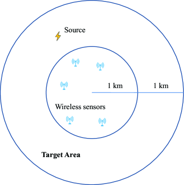
Figure 2: The source and sensor regions in the crowd spectrum sensing example.

we consider a circular area with a radius of $2$ km, within which there is a signal source at an unknown location that may transmit at the frequency band of interest with an unknown power. If the source does not transmit (i.e., the frequency band is not occupied), $\theta=0$; otherwise, $\theta=1$. There are $K$ spectrum sensors, uniformly distributed in a concentric circle with a radius of $1$ km, for detecting whether the source transmits or not. The propagation loss from the source to the sensors is modelled by the CBRS channel model given in [28, pp. 12-13] for distances less than $1$ km and by the Hata model given in [29, Eqn. (A-3)] for distances greater than $1$ km. In both cases, the carrier frequency is fixed at $3625$ MHz, the height of the source antenna is chosen to be $20$ m, and the antenna height of each sensor is chosen to be $1.5$ m.

We assume that the radio receivers in the spectrum sensors suffer only from i.i.d. thermal noise, whose effects on the received power level is modeled by an additive Chi-square distributed component with two degrees of freedom. The source power and noise power are set to $25$ dBm and $-103$ dBm, respectively. The measured power in the decibel scale at each sensor is uniformly quantized to $128$ levels in the range from $-130$ dBm to $-60$ dBm. We also set $m=13$. No information about the locations of the source and sensors, the channel model, and the thermal noise described above is made available to the sensors or the fusion center. Note that the model described above implies that $|\mathcal{X}|=128$, and that $d_{0}=0$ and $d_{1}>0$ with a high probability.

IV-C2 Simulation Results

We consider the two simulation experiments. In the first experiment, we set the number of sensors $K=8$. We select the length of the measurement sequences $t$ from $360$ to $600$ at an increment interval of $20$. We select $30$ groups of random sensor locations and $30$ random source locations uniformly distributed in their respective areas. This set of random locations form $900$ different configurations, from which we obtain the worst-case error probabilities of the first and second types. For each value of $t$ and each configuration of locations, we conduct the detection simulation $7.2\times 10^{6}$ times. For each value of $t$, we find the largest testing threshold $\gamma$ that makes $\lambda_{t}$ no more than $5\times 10^{-4}$, $5\times 10^{-5}$, and $5\times 10^{-6}$ respectively, and record the corresponding values of $-\frac{1}{t}\log_{2}\mu_{t}$. These values serve as estimates of the error exponent of the first type. The results are plotted in Figure 3.

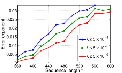
Figure 3: Plots of $-\frac{1}{t}\log_{2}\mu_{t}$ vs. $t$ for different bounds on $\lambda_{t}$.

It can be seen that the value of $-\frac{1}{t}\log_{2}\mu_{t}$ increases as the sequence length $t$ grows, and it levels off as $t$ becomes large. The results indicate that a positive error exponent of the first type is achieved, and thus the condition that $d_{1}>d_{0}$ is valid among the $900$ configurations.

In the second experiment, we fix $t=500$ and consider two different numbers of sensors, $K=7$ and $8$. For both cases, we select $900$ random location configurations as in the first experiment to obtain the worst-cases error probabilities. The receiver operation characteristic (ROC) curves for the cases of $K=7$ and $K=8$ are plotted in Figure 4.

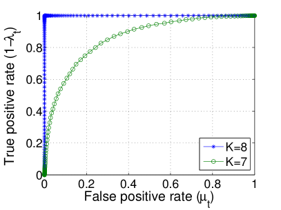
Figure 4: The ROC curves for the networks with 7 and 8 sensors.

For each case, the ROC curve is obtained from $2\times 10^{5}$ simulation runs. It can be seen from the figure that at $t=500$ dropping a single sensor from $K=8$ to $7$ significantly degrade the worst-case detection performance. These results indicate that the error exponents achieved by the test (5) with $K=7$ sensors, albeit may still be positive, seem to be smaller than those achieved by the test (5) with $K=8$ sensors.

V Privacy Analysis

In this section, we present a privacy-preserving performance analysis on the protocol proposed in Section IV based on the attacker-challenger formalism described in Section II-C. The attacker $\mathscr{A}$ is the combined entity consisting of an external eavesdropper, the fusion center, and the set of adversarial sensors as discussed in Section IV-A. Since no knowledge about how many or the identity of the set of adversarial sensors is required for the protocol to operate, we may set $\mathcal{L}=\{K-L+1,K-L+2,\ldots,K\}$ without any loss of generality in the analysis below, where $L$ denotes the number of adversarial sensors. The challenger $\mathscr{C}$, on the other hand, can be thought of as a fictitious entity that maintains the operation of the proposed protocol in that it provides all the available inputs to the attacker in accordance to the protocol. From Section IV, these inputs include the public keys $\mathbf{\Phi}^{n}_{\mathcal{K}\setminus\mathcal{L}}$, the ciphertexts $\mathbf{\bar{C}}_{\mathcal{K}\setminus\mathcal{L},\mathcal{K}}$, and the obfuscated messages $\mathbf{G}_{\mathcal{K}\setminus\mathcal{L}}$ sent by the non-adversarial sensors.

In addition to the above inputs provided by the challenger, the attacker obviously has access to the quantized square-root types $\mathbf{Q}_{\mathcal{L}}$ observed by the adversarial sensors as well as the key pairs $(\mathbf{\Phi}^{n}_{\mathcal{L}},\mathbf{\Psi}^{n}_{\mathcal{L}})$, the secret random numbers $\mathbf{R}_{\mathcal{L},\mathcal{K}}$, the ciphertexts $\mathbf{\bar{C}}_{\mathcal{L},\mathcal{K}}$, and the obfuscated messages $\mathbf{G}_{\mathcal{L}}$ generated by themselves. The goal of the attacker is to produce an estimate of the square-root types $\mathbf{Q}_{\mathcal{K}\setminus\mathcal{L}}$ observed by the non-adversarial sensors from all available information described above. The attacker does not need to follow the exact steps in the protocol proposed in Section IV as long as any deviations must not disrupt proper execution of the test in (5). Specifically, we allow the adversarial sensors in Phase:

1. to wait until receiving the public keys $\mathbf{\Phi}^{n}_{\mathcal{K}\setminus\mathcal{L}}$ from the non-adversarial sensors before generating their key pairs as any general PPT functions of $\mathbf{\Phi}^{n}_{\mathcal{K}\setminus\mathcal{L}}$, i.e.,

   $$(\mathbf{\Phi}^{n}_{\mathcal{L}},\mathbf{\Psi}^{n}_{\mathcal{L}})=(\mathbf{\Phi}^{n}_{\mathcal{L}}(\mathbf{\Phi}^{n}_{\mathcal{K}\setminus\mathcal{L}}),\mathbf{\Psi}^{n}_{\mathcal{L}}(\mathbf{\Phi}^{n}_{\mathcal{K}\setminus\mathcal{L}})),$$ (16)

2. to wait until receiving the ciphertexts $\mathbf{\bar{C}}_{\mathcal{K}\setminus\mathcal{L},\mathcal{K}}$ from the non-adversarial sensors and decrypting to obtain $\mathbf{R}_{\mathcal{K}\setminus\mathcal{L},\mathcal{L}}$ before generating their random numbers as any general PPT functions of the information they possess up to that point, i.e.,

   $$\mathbf{R}_{\mathcal{L},\mathcal{K}}=\mathbf{R}_{\mathcal{L},\mathcal{K}}(\mathbf{Q}_{\mathcal{L}},\mathbf{\Phi}^{n}_{\mathcal{K}},\mathbf{\Psi}^{n}_{\mathcal{L}},\mathbf{\bar{C}}_{\mathcal{K}\setminus\mathcal{L},\mathcal{K}},\mathbf{R}_{\mathcal{K}\setminus\mathcal{L},\mathcal{L}})$$ (17)

   with the restriction that (10) must be satisfied for all $R_{l,l}$ where $l\in\mathcal{L}$, and

3. to use all information available at the end of the protocol in any general PPT estimator for $\mathbf{Q}_{\mathcal{K}\setminus\mathcal{L}}$, i.e.,

   $$\mathbf{\hat{Q}}_{\mathcal{K}\setminus\mathcal{L}}=$$

   $$\mathbf{\hat{Q}}_{\mathcal{K}\setminus\mathcal{L}}(\mathbf{Q}_{\mathcal{L}},\mathbf{\Phi}^{n}_{\mathcal{K}},\mathbf{\Psi}^{n}_{\mathcal{L}},\mathbf{\bar{C}}_{\mathcal{K},\mathcal{K}},\mathbf{G}_{\mathcal{K}},\mathbf{R}_{\mathcal{L},\mathcal{K}},\mathbf{R}_{\mathcal{K}\setminus\mathcal{L},\mathcal{L}})$$ (18)

   with the restriction that (11) must be satisfied for all $G_{l}$ where $l\in\mathcal{L}$.

V-A Main Result

Consider the following type estimation attack (TEA) experiment, as shown in Figure 5, between the attacker $\mathscr{A}$ and her challenger $\mathscr{C}$ as specified above:

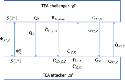
Figure 5: The TEA experiment.

1. For each $k\in\mathcal{K}\setminus\mathcal{L}$, $\mathscr{C}$ runs $S(1^{n})$ to get the pair of public key $\Phi_{k}^{n}\in\mathcal{E}_{n}$ and private key $\Psi_{k}^{n}\in\mathcal{D}_{n}$. Then, $\mathscr{C}$ gives $\boldsymbol{\Phi}_{\mathcal{K}\setminus\mathcal{L}}^{n}$ to $\mathscr{A}$. Then, $\mathscr{A}$ generates the set of key pairs $(\boldsymbol{\Phi}_{\mathcal{L}}^{n},\boldsymbol{\Psi}_{\mathcal{L}}^{n})$ according to (16), and gives $\boldsymbol{\Phi}_{\mathcal{L}}^{n}$ to $\mathscr{C}$.

2. $\mathscr{C}$ draws a collection of quantized square-root types $\mathbf{Q}_{\mathcal{K}}\in\mathcal{Q}^{K}_{t}(\mathcal{X})$ according to the distribution $p_{\mathbf{Q}_{\mathcal{K}}}(\cdot;\theta)$, and gives $\mathbf{Q}_{\mathcal{L}}$ to $\mathscr{A}$. We assume that $\mathscr{A}$ also knows the value of the system state $\theta\in\{0,1\}$ and the distribution $p_{\mathbf{Q}_{\mathcal{K}}}(\cdot;\theta)$. Hence, we will simply write $p_{\mathbf{Q}_{\mathcal{K}}}(\cdot)$ in place of $p_{\mathbf{Q}_{\mathcal{K}}}(\cdot;\theta)$ in the discussion below to simplify notation.

3. $\mathscr{C}$ generates $\mathbf{R}_{\mathcal{K}\setminus\mathcal{L},\mathcal{K}}$ with $\mathbf{R}_{k,l}$ i.i.d. $\sim{u}(\mathcal{N}_{m}^{|\mathcal{X}|})$ for $k\neq l$, and $\mathbf{R}_{k,k}=\ominus\bigoplus_{l\in\mathcal{K}\setminus k}\mathbf{R}_{k,l}$ according to (10). Then, $\mathscr{C}$ computes ${\mathbf{\bar{C}}}_{\mathcal{K}\setminus\mathcal{L},\mathcal{K}}={E}({\mathbf{\bar{R}}}_{\mathcal{K}\setminus\mathcal{L},\mathcal{K}};\mathbf{\Phi}^{n}_{\mathcal{K}})$, and gives it to $\mathscr{A}$.

4. After receiving ${\mathbf{\bar{C}}}_{\mathcal{K}\setminus\mathcal{L},\mathcal{K}}$, $\mathscr{A}$ decrypts to get $\mathbf{R}_{\mathcal{K}\setminus\mathcal{L},\mathcal{L}}=D(\mathbf{C}_{\mathcal{K}\setminus\mathcal{L},\mathcal{L}};\mathbf{\Psi}^{n}_{\mathcal{L}})$, and generates $\mathbf{R}_{\mathcal{L},\mathcal{K}}$ according to (17). Then, $\mathscr{A}$ computes ${\mathbf{\bar{C}}}_{\mathcal{L},\mathcal{K}}=E({\mathbf{\bar{R}}}_{\mathcal{L},\mathcal{K}};\mathbf{\Phi}^{n}_{\mathcal{K}})$, and gives $\mathbf{\bar{C}}_{\mathcal{L},\mathcal{K}}$ to $\mathscr{C}$.

5. $\mathscr{C}$ calculates $\mathbf{R}_{\mathcal{L},\mathcal{K}\setminus\mathcal{L}}=D(\mathbf{C}_{\mathcal{L},\mathcal{K}\setminus\mathcal{L}};\mathbf{\Psi}^{n}_{\mathcal{K}\setminus\mathcal{L}})$, computes $\mathbf{G}_{\mathcal{K}\backslash\mathcal{L}}=\mathbf{Q}_{\mathcal{K}\setminus\mathcal{L}}\oplus\mathbf{\Sigma}_{\mathbf{R}_{\mathcal{K},\mathcal{K}\setminus\mathcal{L}}}$ according to (11), and gives $\mathbf{G}_{\mathcal{K}\setminus\mathcal{L}}$ to $\mathscr{A}$.

6. $\mathscr{A}$ computes $\mathbf{G}_{\mathcal{L}}=\mathbf{Q}_{\mathcal{L}}\oplus\mathbf{\Sigma}_{\mathbf{R}_{\mathcal{K},\mathcal{L}}}$ according to (11). Then, according to (18), $\mathscr{A}$ generates, and reports to $\mathscr{C}$, ${\mathbf{\hat{Q}}}_{\mathcal{K}\setminus\mathcal{L}}$ as her estimate of $\mathbf{Q}_{\mathcal{K}\setminus\mathcal{L}}$.

Note that in step 2) above the distribution $p_{\mathbf{Q}_{\mathcal{K}}}(\cdot;\theta)$ models two different physical mechanisms that give rise to the randomness of $\mathbf{Q}_{\mathcal{K}}$. The first mechanism is the choice of $\mathbf{p}_{\theta,\mathcal{K}}$, which is a random instantiation from some underlying random model that characterizes attributes, such as the locations as in the example of Section IV-C, of the sensors. A more conservative deterministic approach is adopted in the formulation of the event detection problem in Section III by treating $\mathbf{p}_{\theta,\mathcal{K}}$ as fixed and considering the worst-case detection errors. It is more convenient to consider a random model for privacy analysis here. The second mechanism is the random instantiation of $\mathbf{X}_{\mathcal{K}}$, of which $\mathbf{Q}_{\mathcal{K}}$ is a function, from $\mathbf{p}_{\theta,\mathcal{K}}$. This mechanism is modeled in exactly the same way in the detection problem.

For any radius $\tau\geq 0$ and $\mathbf{q}_{\mathcal{K}\setminus\mathcal{L}}\in\mathcal{Q}^{K-L}_{t}(\mathcal{X})$, define a neighborhood of quantized square root types around $\mathbf{q}_{\mathcal{K}\setminus\mathcal{L}}$:

$$\mathcal{N}_{\tau}(\mathbf{q}_{\mathcal{K}\setminus\mathcal{L}}) =\big{\{}\mathbf{q}^{\prime}_{\mathcal{K}\setminus\mathcal{L}}\in\mathcal{Q}^{K-L}_{t}(\mathcal{X}):d_{H}(\mathbf{q}^{\prime 2}_{\mathcal{K}\setminus\mathcal{L}},\mathbf{q}^{2}_{\mathcal{K}\setminus\mathcal{L}})\leq\tau,$$

$$\hskip 20.0pt\boldsymbol{\Sigma}_{\mathbf{q}^{\prime}_{\mathcal{K}\setminus\mathcal{L}}}=\boldsymbol{\Sigma}_{\mathbf{q}_{\mathcal{K}\setminus\mathcal{L}}}\big{\}}$$

where $\mathbf{q}^{2}_{\mathcal{K}\setminus\mathcal{L}}$ denotes elementwise squaring of the vector $\mathbf{q}_{\mathcal{K}\setminus\mathcal{L}}$. Then, we say $\mathscr{A}$ wins the TEA experiment if ${\mathbf{\hat{Q}}}_{\mathcal{K}\setminus\mathcal{L}}$ is within a small neighborhood around $\mathbf{Q}_{\mathcal{K}\setminus\mathcal{L}}$, i.e., ${\mathbf{\hat{Q}}}_{\mathcal{K}\setminus\mathcal{L}}\in\mathcal{N}_{\tau}(\mathbf{Q}_{\mathcal{K}\setminus\mathcal{L}})$.

Theorem 7.

Let $\mathbf{\hat{Q}}_{\mathcal{K}\setminus\mathcal{L}}$ be the estimator for ${\mathbf{Q}}_{\mathcal{K}\setminus\mathcal{L}}$ of any PPT attacker $\mathscr{A}$ in the TEA experiment above. Given $[\boldsymbol{\Sigma}_{\mathbf{Q}_{\mathcal{K}\setminus\mathcal{L}}},\mathbf{Q}_{\mathcal{L}}]$, let ${\mathbf{\hat{Q}}}^{\prime}_{\mathcal{K}\setminus\mathcal{L}}$ be another estimator that has the same conditional distribution as ${\mathbf{\hat{Q}}}_{\mathcal{K}\setminus\mathcal{L}}$ but is conditionally independent of ${\mathbf{Q}}_{\mathcal{K}\setminus\mathcal{L}}$. If $L\leq K-2$, then for any $\tau\geq 0$, $\boldsymbol{\sigma}\in\mathcal{N}_{m}^{|\mathcal{X}|}$, $\mathbf{q}_{\mathcal{L}}\in\mathcal{Q}_{t}^{L}(\mathcal{X})$,

$$\Pr(\mathbf{\hat{Q}}_{\mathcal{K}\setminus\mathcal{L}}\in\mathcal{N}_{\tau}(\mathbf{Q}_{\mathcal{K}\backslash\mathcal{L}})\mid\boldsymbol{\Sigma}_{\mathbf{Q}_{\mathcal{K}\backslash\mathcal{L}}}=\boldsymbol{\sigma},\mathbf{Q}_{\mathcal{L}}=\mathbf{q}_{\mathcal{L}})$$

$$\leq \Pr(\mathbf{\hat{Q}}^{\prime}_{\mathcal{K}\setminus\mathcal{L}}\in\mathcal{N}_{\tau}(\mathbf{Q}_{\mathcal{K}\backslash\mathcal{L}})\mid\boldsymbol{\Sigma}_{\mathbf{Q}_{\mathcal{K}\backslash\mathcal{L}}}=\boldsymbol{\sigma},\mathbf{Q}_{\mathcal{L}}=\mathbf{q}_{\mathcal{L}})$$

$$+8(K-L-1)|\mathcal{X}|\cdot F_{\mathrm{CPA}}(n)$$ (19)

where $F_{\mathrm{CPA}}(n)$, given in (3), is the probability advantage of an attacker in the CPA experiment against the public-key cryptographic scheme $\Pi$ with security parameter $n$.

The theorem guarantees that as long as the public-key cryptographic scheme $\Pi$ employed is CPA-secure, any PPT attacker can not do much better than independently guessing the value of ${\mathbf{Q}}_{\mathcal{K}\setminus\mathcal{L}}$ given her own information $\mathbf{Q}_{\mathcal{L}}$ from the adversarial sensors and the information $\boldsymbol{\Sigma}_{\mathbf{Q}_{\mathcal{K}\backslash\mathcal{L}}}$ “leaked” to her via the proposed protocol. One may further quantify the notion of “not much better” above, by noting that since $\mathcal{Q}^{K-L}_{t}(\mathcal{X})$ has at most $(t+1)^{(K-L)|\mathcal{X}|}$ elements, we must have

$$\max_{\mathbf{\hat{Q}}^{\prime}_{\mathcal{K}\setminus\mathcal{L}}}\Pr(\mathbf{\hat{Q}}^{\prime}_{\mathcal{K}\setminus\mathcal{L}}\in\mathcal{N}_{\tau}(\mathbf{Q}_{\mathcal{K}\backslash\mathcal{L}})\mid\boldsymbol{\Sigma}_{\mathbf{Q}_{\mathcal{K}\backslash\mathcal{L}}}=\boldsymbol{\sigma},\mathbf{Q}_{\mathcal{L}}=\mathbf{q}_{\mathcal{L}})$$

$$\geq(t+1)^{-(K-L)|\mathcal{X}|}.$$

If $\Pi$ is CPA-secure, then it suffices to choose $n=\mathcal{O}(t^{\frac{(K-L)|\mathcal{X}|}{\rho}})$, for any $\rho>1$, to make the bound in (19) non-trivial.

The main idea of the proof of Theorem 7 is to first reduce the TEA experiment to a type discrimination attack (TDA) experiment in which the attacker aims to distinguish between a pair of quantized square-root types instead. The TDA experiment is then further decomposed into two CPA experiments and a third one involving only secret random numbers. The advantage equation in (19) is obtained from the advantages of the experiments in the chain of reduction steps mentioned. We will construct the proof step by step in the rest of this section.

V-B Useful Lemmas

Before proceeding to construct the proof of Theorem 7, we state here a few lemmas that help to simplify later discussions. As the proofs of these lemmas are either trivial or technical rather than illustrative, they are provided for completeness in Appendix B.

Lemma 8.

Suppose $L\leq K-2$. Let $\mathcal{I}=\{1,2\}\subseteq\mathcal{K}\setminus\mathcal{L}$, and $\mathbf{R}_{\mathcal{I},\mathcal{K}}=[\mathbf{R}_{k,l}]_{k\in\mathcal{I},l\in\mathcal{K}}$ be a collection of random variables satisfying $\mathbf{R}_{k,l}$ i.i.d. $\sim{u}(\mathcal{N}_{m}^{|\mathcal{X}|})$ for $k\neq l$, and $\mathbf{R}_{k,k}=\ominus\bigoplus_{j\in\mathcal{K}\setminus k}\mathbf{R}_{k,j}$ according to (10). Then, for any $\mathbf{r}_{\mathcal{I},\mathcal{L}}\in\mathcal{N}_{m}^{2L|\mathcal{X}|}$ and $\boldsymbol{\sigma}_{\mathcal{K}\setminus\mathcal{L}}\in\mathcal{N}_{m}^{(K-L)|\mathcal{X}|}$,

$$P_{\boldsymbol{\Sigma}_{\mathbf{R}_{\mathcal{I},\mathcal{K}\setminus\mathcal{L}}}\mid\mathbf{R}_{\mathcal{I},\mathcal{L}}}(\boldsymbol{\sigma}_{\mathcal{K}\setminus\mathcal{L}}\mid\mathbf{r}_{\mathcal{I},\mathcal{L}})$$

$$=2^{-m(K-L-1)|\mathcal{X}|}\cdot\delta\left(\boldsymbol{\Sigma}_{\boldsymbol{\sigma}_{\mathcal{K}\setminus\mathcal{L}}}\oplus\bigoplus_{l\in\mathcal{L}}\boldsymbol{\Sigma}_{\mathbf{r}_{\mathcal{I},l}}\right).$$ (20)

Lemma 9.

Let $B\in\{0,1\}$, $Y\in\mathcal{Y}$, $U\in\mathcal{U}$, $V\in\mathcal{V}$, and $W\in\mathcal{W}$ be discrete random variables. Let $\hat{B}(Y,V,W)$ be a PPT estimator of $B$. If $W$ is conditionally independent of $B$ given $[Y,U,V]$ and $W=W(Y,U,V)$ can be generated by a PPT algorithm, then the estimator $\hat{B}_{0}(Y,U,V)=\hat{B}(Y,V,W(Y,U,V))$ is PPT, and for any $(u,v)\in\mathcal{U}\times\mathcal{V}$,

$$\Pr(\hat{B}_{0}(Y,U,V)=B\mid U=u,V=v)$$

$$=\Pr(\hat{B}(Y,V,W)=B\mid U=u,V=v).$$ (21)

Lemma 10.

Let $Z_{1}\in\mathcal{Z}_{1}$, $Z_{2}\in\mathcal{Z}_{2}$, $Z_{3}\in\mathcal{Z}_{3}$, and $W=W(Z_{1},Z_{2})\in\mathcal{W}$ be discrete random variables. If $Z_{1}$ is conditionally independent of $Z_{3}$ given $Z_{2}$, then $W$ is conditionally independent of $Z_{3}$ given $Z_{2}$.

V-C Multi-Encryption CPA Experiment

Recall that the privacy-preserving protocol in Section IV requires each of the $K$ sensors to send multiple ciphertexts to other sensors. Thus, to prove Theorem 7, we need to extend the CPA experiment described in Section II-C to the multi-sensor, multi-message setting of $K$ sensors, each encrypting $M_{k}$ messages (plaintexts), and $M=\sum_{k=1}^{K}M_{k}$:

1. The challenger runs $S(1^{n})$ to generate the pair of public key $\Phi_{k}^{n}\in\mathcal{E}_{n}$ and private key $\Psi_{k}^{n}\in\mathcal{D}_{n}$, for each $k\in\mathcal{K}$. The challenger gives the set of public keys $\boldsymbol{\Phi}_{\mathcal{K}}^{n}$ to the attacker.

2. The attacker generates two collections of challenge messages $\mathbf{R}^{0}_{\mathcal{K}}=[[R_{k,i}^{0}]_{i=1}^{M_{k}}]_{k=1}^{K}$ and $\mathbf{R}^{1}_{\mathcal{K}}=[[R_{k,i}^{1}]_{i=1}^{M_{k}}]_{k=1}^{K}$, where $R_{k,i}^{0}$ and $R_{k,i}^{1}$ are i.i.d. $\sim u(\mathcal{N}_{m})$ for all $k\in\mathcal{K}$ and $i=1,2,\ldots,M_{k}$. The attacker gives $\mathbf{R}^{0}_{\mathcal{K}}$ and $\mathbf{R}^{1}_{\mathcal{K}}$ to the challenger.

3. The challenger generates an independent random bit $B=\{0,1\}$ with equal probabilities, computes the ciphertext collection $\mathbf{C}^{B}_{\mathcal{K}}=[[{E}(R_{k,i}^{B};\Phi_{k}^{n})]_{i=1}^{M_{k}}]_{k=1}^{K}\in\mathcal{C}^{M}$, and gives it to the attacker.

4. The attacker uses the estimator $\hat{B}=\hat{B}(\mathbf{C}^{B}_{\mathcal{K}},\mathbf{R}^{0}_{\mathcal{K}},\mathbf{R}^{1}_{\mathcal{K}},\mathbf{\Phi}^{n}_{\mathcal{K}})$ to output her estimate of $B$, and reports $\hat{B}$ to the challenger.

If $\hat{B}=B$, then the attacker wins the multi-encryption CPA experiment. The following lemma expresses the winning probability advantage of the multi-encryption CPA attacker in terms of that of a CPA attacker:

Lemma 11.

For any PPT attacker in the multi-encryption CPA experiment described above,

$$\Pr(\hat{B}=B)-\frac{1}{2}\leq M\cdot F_{\mathrm{CPA}}(n).$$ (22)

Proof.

Based on Assumption 4, the reduction approach in [30] can be directly used here to establish the lemma. ∎

V-D Type Discrimination Attack (TDA)

The proof of Theorem 7 relies on a simpler version of the TEA experiment in which the attacker tries to distinguish between a pair of quantized square-root types instead. We refer to this simpler experiment as the type discrimination attack (TDA) experiment. The steps of the TDA experiment between the attacker $\mathscr{A}^{\prime}$ and her challenger $\mathscr{C}^{\prime}$, as shown in Figure 6, are as follows:

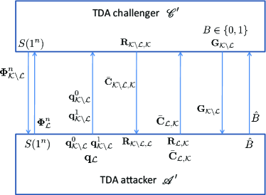
Figure 6: The TDA experiment

1. Same as step 1) of the TEA experiment with $\mathscr{A}^{\prime}$ and $\mathscr{C}^{\prime}$ taking the roles of $\mathscr{A}$ and $\mathscr{C}$, respectively.

2. $\mathscr{A}^{\prime}$ selects three collections of quantized square-root types: $\mathbf{q}_{\mathcal{L}}\in\mathcal{Q}_{t}^{L}(\mathcal{X})$, $\mathbf{q}^{0}_{\mathcal{K}\setminus\mathcal{L}}\in\mathcal{Q}^{K-L}_{t}(\mathcal{X})$, and $\mathbf{q}^{1}_{\mathcal{K}\setminus\mathcal{L}}\in\mathcal{Q}^{K-L}_{t}(\mathcal{X})$ satisfying $\mathbf{\Sigma}_{\mathbf{q}^{0}_{\mathcal{K}\setminus\mathcal{L}}}=\mathbf{\Sigma}_{\mathbf{q}^{1}_{\mathcal{K}\setminus\mathcal{L}}}$. $\mathscr{A}^{\prime}$ gives $[\mathbf{q}^{0}_{\mathcal{K}\setminus\mathcal{L}},\mathbf{q}^{1}_{\mathcal{K}\setminus\mathcal{L}}]$ to $\mathscr{C}^{\prime}$.

3. Same as step 3) of the TEA experiment with $\mathscr{A}^{\prime}$ and $\mathscr{C}^{\prime}$ taking the roles of $\mathscr{A}$ and $\mathscr{C}$, respectively.

4. Same as step 4) of the TEA experiment with $\mathscr{A}^{\prime}$ and $\mathscr{C}^{\prime}$ taking the roles of $\mathscr{A}$ and $\mathscr{C}$, respectively.

5. $\mathscr{C}^{\prime}$ calculates $\mathbf{R}_{\mathcal{L},\mathcal{K}\setminus\mathcal{L}}=D(\mathbf{C}_{\mathcal{L},\mathcal{K}\setminus\mathcal{L}};\mathbf{\Psi}^{n}_{\mathcal{K}\setminus\mathcal{L}})$, generates an independent random bit $B\in\{0,1\}$ with equal probabilities, computes $\mathbf{G}^{B}_{\mathcal{K}\setminus\mathcal{L}}=\mathbf{q}^{B}_{\mathcal{K}\backslash\mathcal{L}}\oplus\mathbf{\Sigma}_{\mathbf{R}_{\mathcal{K},\mathcal{K}\setminus\mathcal{L}}}$, and gives $\mathbf{G}^{B}_{\mathcal{K}\setminus\mathcal{L}}$ to $\mathscr{A}^{\prime}$.

6. $\mathscr{A}^{\prime}$ estimates $B$ using the estimator $\hat{B}=\hat{B}(\mathbf{q}^{0}_{\mathcal{K}\setminus\mathcal{L}},\\ \mathbf{q}^{1}_{\mathcal{K}\setminus\mathcal{L}},\mathbf{q}_{\mathcal{L}},{\mathbf{\bar{C}}}_{\mathcal{K},\mathcal{K}},\mathbf{G}^{B}_{\mathcal{K}\setminus\mathcal{L}},\mathbf{R}_{\mathcal{L},\mathcal{K}},\mathbf{R}_{\mathcal{K}\setminus\mathcal{L},\mathcal{L}},\mathbf{\Phi}^{n}_{\mathcal{K}},\mathbf{\Psi}^{n}_{\mathcal{L}})$, and reports $\hat{B}$ to $\mathscr{C}^{\prime}$.

If $\hat{B}=B$, it is said that $\mathscr{A}^{\prime}$ wins the TDA experiment. The following lemma expresses the winning probability advantage of the TDA attacker in terms of that of a CPA attacker:

Lemma 12.

Suppose $L\leq K-2$. For any PPT attacker in the TDA experiment described above, $\mathbf{q}_{\mathcal{L}}\in\mathcal{Q}^{L}_{t}(\mathcal{X})$, and $\mathbf{q}^{0}_{\mathcal{K}\setminus\mathcal{L}},\mathbf{q}^{1}_{\mathcal{K}\setminus\mathcal{L}}\in\mathcal{Q}^{K-L}_{t}(\mathcal{X})$ satisfying $\mathbf{\Sigma}_{\mathbf{q}^{0}_{\mathcal{K}\setminus\mathcal{L}}}=\mathbf{\Sigma}_{\mathbf{q}^{1}_{\mathcal{K}\setminus\mathcal{L}}}$,

$$\Pr(\hat{B}=B\mid\mathbf{Q}^{0}_{\mathcal{K}\setminus\mathcal{L}}=\mathbf{q}^{0}_{\mathcal{K}\setminus\mathcal{L}},\mathbf{Q}^{1}_{\mathcal{K}\setminus\mathcal{L}}=\mathbf{q}^{1}_{\mathcal{K}\setminus\mathcal{L}},\mathbf{Q}_{\mathcal{L}}=\mathbf{q}_{\mathcal{L}})$$

$$\leq\frac{1}{2}+4(K-L-1)|\mathcal{X}|\cdot F_{\mathrm{CPA}}(n).$$ (23)

Proof.

The main idea of the proof is to use the TDA attacker $\mathscr{A}^{\prime}$ to construct three attackers in three new experiments. The first two experiments can be reduced to multi-encryption CPA experiments by way of Lemma 9. Thus, Lemma 11 gives the probability advantages of the attackers in these two experiments. On the other hand, the probability advantage of the attacker winning the third experiment can be analyzed using Lemma 8. Then, the probability advantage of $\mathscr{A}^{\prime}$ winning her TDA experiment can be derived from the probability advantages of the new attackers winning their respective experiments. For convenience, we write $\mathcal{I}=\{1,2\}$ and $\mathcal{J}=\mathcal{K}\setminus(\mathcal{I}\cup\mathcal{L})$ throughout the rest of the proof.

As shown in Figure 7, we construct the first experiment with attacker $\mathscr{A}_{1}$ and challenger $\mathscr{C}_{1}$ as follows:

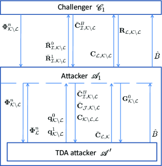
Figure 7: The first constructed experiment for proving Lemma 12

1. $\mathscr{C}_{1}$ runs $S(1^{n})$ to get the key pair collection $(\boldsymbol{\Phi}^{n}_{\mathcal{K}\setminus\mathcal{L}},\boldsymbol{\Psi}^{n}_{\mathcal{K}\setminus\mathcal{L}})$, and gives $\boldsymbol{\Phi}^{n}_{\mathcal{K}\setminus\mathcal{L}}$ to $\mathscr{A}_{1}$, who passes it on to $\mathscr{A}^{\prime}$. Then, $\mathscr{A}^{\prime}$ generates the set of key pairs $(\boldsymbol{\Phi}_{\mathcal{L}}^{n},\boldsymbol{\Psi}_{\mathcal{L}}^{n})$ according to (16), and gives $\boldsymbol{\Phi}_{\mathcal{L}}^{n}$ to $\mathscr{A}_{1}$.

2. $\mathscr{A}^{\prime}$ selects $\mathbf{q}_{\mathcal{L}}$, $\mathbf{q}^{0}_{\mathcal{K}\setminus\mathcal{L}}$, and $\mathbf{q}^{1}_{\mathcal{K}\setminus\mathcal{L}}$ as in step 2) of the TDA experiment, and then passes $[\mathbf{q}^{0}_{\mathcal{K}\setminus\mathcal{L}},\mathbf{q}^{1}_{\mathcal{K}\setminus\mathcal{L}}]$ to $\mathscr{A}_{1}$.

3. $\mathscr{A}_{1}$ generates $\mathbf{R}_{\mathcal{K}\setminus\mathcal{L},\mathcal{K}}$ with $\mathbf{R}_{k,l}$ i.i.d. $\sim\mathcal{U}(\mathcal{N}_{m}^{|\mathcal{X}|})$ for $k\neq l$, and $\mathbf{R}_{k,k}=\ominus\bigoplus_{l\in\mathcal{K}\setminus k}\mathbf{R}_{k,l}$ according to (10). Then, $\mathscr{A}_{1}$ sets ${\mathbf{\bar{R}}}^{0}_{\mathcal{I},\mathcal{K}\setminus\mathcal{L}}={\mathbf{\bar{R}}}_{\mathcal{I},\mathcal{K}\setminus\mathcal{L}}$ and ${\mathbf{\bar{R}}}^{1}_{\mathcal{I},\mathcal{K}\setminus\mathcal{L}}=0^{2(K-L-1)|\mathcal{X}|}$, and gives these two collections to $\mathscr{C}_{1}$.

4. $\mathscr{C}_{1}$ selects an independent bit $B\in\{0,1\}$ with equal probabilities, computes ${\mathbf{\bar{C}}}^{B}_{\mathcal{I},\mathcal{K}\setminus\mathcal{L}}=E({\mathbf{\bar{R}}}^{B}_{\mathcal{I},\mathcal{K}\setminus\mathcal{L}};\boldsymbol{\Phi}^{n}_{\mathcal{K}\setminus\mathcal{L}})$, and gives ${\mathbf{\bar{C}}}^{B}_{\mathcal{I},\mathcal{K}\setminus\mathcal{L}}$ to $\mathscr{A}_{1}$.

5. $\mathscr{A}_{1}$ computes ${\mathbf{\bar{C}}}_{\mathcal{J},\mathcal{K}\setminus\mathcal{L}}=E({\mathbf{\bar{R}}}_{\mathcal{J},\mathcal{K}\setminus\mathcal{L}};\boldsymbol{\Phi}^{n}_{\mathcal{K}\setminus\mathcal{L}})$, $\mathbf{C}_{\mathcal{K}\setminus\mathcal{L},\mathcal{L}}=E(\mathbf{R}_{\mathcal{K}\setminus\mathcal{L},\mathcal{L}};\boldsymbol{\Phi}^{n}_{\mathcal{L}})$, and gives ${\mathbf{\bar{C}}}^{B}_{\mathcal{I},\mathcal{K}\setminus\mathcal{L}}$, ${\mathbf{\bar{C}}}_{\mathcal{J},\mathcal{K}\setminus\mathcal{L}}$, and $\mathbf{C}_{\mathcal{K}\setminus\mathcal{L},\mathcal{L}}$ to $\mathscr{A}^{\prime}$.

6. $\mathscr{A}^{\prime}$ follows step 4) of the TDA experiment to decrypt $\mathbf{C}_{\mathcal{K}\setminus\mathcal{L},\mathcal{L}}$, generate $\mathbf{R}_{\mathcal{L},\mathcal{K}}$, encrypt to obtain $\mathbf{\bar{C}}_{\mathcal{L},\mathcal{K}}$, and send $\mathbf{\bar{C}}_{\mathcal{L},\mathcal{K}}$ to $\mathscr{A}_{1}$, who then passes on $\mathbf{C}_{\mathcal{L},\mathcal{K}\setminus\mathcal{L}}$ to $\mathscr{C}_{1}$.

7. $\mathscr{C}_{1}$ calculates $\mathbf{R}_{\mathcal{L},\mathcal{K}\setminus\mathcal{L}}=D(\mathbf{C}_{\mathcal{L},\mathcal{K}\setminus\mathcal{L}};\mathbf{\Psi}^{n}_{\mathcal{K}\setminus\mathcal{L}})$ and sends $\mathbf{R}_{\mathcal{L},\mathcal{K}\setminus\mathcal{L}}$ to $\mathscr{A}_{1}$.

8. $\mathscr{A}_{1}$ computes $\mathbf{G}^{0}_{\mathcal{K}\setminus\mathcal{L}}=\mathbf{q}^{0}_{\mathcal{K}\setminus\mathcal{L}}\oplus\mathbf{\Sigma}_{\mathbf{R}_{\mathcal{K},\mathcal{K}\setminus\mathcal{L}}}$, and gives $\mathbf{G}^{0}_{\mathcal{K}\setminus\mathcal{L}}$ to $\mathscr{A}^{\prime}$.

9. $\mathscr{A}^{\prime}$ uses $\hat{B}=\hat{B}(\mathbf{q}^{0}_{\mathcal{K}\setminus\mathcal{L}},\mathbf{q}^{1}_{\mathcal{K}\setminus\mathcal{L}},\mathbf{q}_{\mathcal{L}},[\mathbf{\bar{C}}^{B}_{\mathcal{I},\mathcal{K}\setminus\mathcal{L}},\mathbf{\bar{C}}_{\mathcal{J},\mathcal{K}\setminus\mathcal{L}},\\ \mathbf{C}_{\mathcal{K}\setminus\mathcal{L},\mathcal{L}},\mathbf{\bar{C}}_{\mathcal{L},\mathcal{K}}],\mathbf{G}^{0}_{\mathcal{K}\setminus\mathcal{L}},\mathbf{R}_{\mathcal{L},\mathcal{K}},\mathbf{R}_{\mathcal{K}\setminus\mathcal{L},\mathcal{L}},\boldsymbol{\Phi}^{n}_{\mathcal{K}},\boldsymbol{\Psi}^{n}_{\mathcal{L}})$ in step 6) of the TDA experiment with the input arguments as specified to estimate $B$, and reports $\hat{B}$ to $\mathscr{A}_{1}$, who passes it on to $\mathscr{C}_{1}$.

We will use Lemmas 9 and 10 below. To match the notation in the lemmas, let $\mathbf{Q}^{0}_{\mathcal{K}\setminus\mathcal{L}}\sim\delta_{\mathbf{q}^{0}_{\mathcal{K}\setminus\mathcal{L}}}$, $\mathbf{Q}^{1}_{\mathcal{K}\setminus\mathcal{L}}\sim\delta_{\mathbf{q}^{1}_{\mathcal{K}\setminus\mathcal{L}}}$, $\mathbf{Q}_{\mathcal{L}}\sim\delta_{\mathbf{q}_{\mathcal{L}}}$, $Y={\mathbf{\bar{C}}}^{B}_{\mathcal{I},\mathcal{K}\setminus\mathcal{L}}$, $U={\mathbf{\bar{R}}}_{\mathcal{I},\mathcal{K}\setminus\mathcal{L}}$, $V=\boldsymbol{\Phi}^{n}_{\mathcal{K}\setminus\mathcal{L}}$, $Z_{0}=[\mathbf{Q}^{0}_{\mathcal{K}\setminus\mathcal{L}},\mathbf{Q}^{1}_{\mathcal{K}\setminus\mathcal{L}},\mathbf{Q}_{\mathcal{L}},{\mathbf{\bar{C}}}_{\mathcal{J},\mathcal{K}\setminus\mathcal{L}},\mathbf{C}_{\mathcal{K}\setminus\mathcal{L},\mathcal{L}},\mathbf{R}_{\mathcal{K}\setminus\mathcal{L},\mathcal{L}},\boldsymbol{\Phi}^{n}_{\mathcal{L}},\boldsymbol{\Psi}^{n}_{\mathcal{L}}]$, $Z_{1}=[Z_{0},{\mathbf{\bar{R}}}_{\mathcal{J},\mathcal{K}\setminus\mathcal{L}}]$, $Z_{2}=[Y,U,V]$, and $W=[{\mathbf{\bar{C}}}_{\mathcal{L},\mathcal{K}},\mathbf{G}^{0}_{\mathcal{K}\setminus\mathcal{L}},\\ \mathbf{R}_{\mathcal{L},\mathcal{K}},Z_{0}]$.

Note that ${\mathbf{\bar{C}}}_{\mathcal{L},\mathcal{K}}=E({\mathbf{\bar{R}}}_{\mathcal{L},\mathcal{K}};\boldsymbol{\Phi}^{n}_{\mathcal{K}})$, $\mathbf{G}^{0}_{\mathcal{K}\setminus\mathcal{L}}$ is a function of $[\mathbf{Q}^{0}_{\mathcal{K}\setminus\mathcal{L}},{\mathbf{\bar{R}}}_{\mathcal{K}\setminus\mathcal{L},\mathcal{K}},\mathbf{R}_{\mathcal{L},\mathcal{K}\setminus\mathcal{L}}]$, and $\mathbf{R}_{\mathcal{L},\mathcal{K}}$ is a function of $[\mathbf{Q}_{\mathcal{L}},\mathbf{\Phi}^{n}_{\mathcal{K}},\mathbf{\Psi}^{n}_{\mathcal{L}},\\ {\mathbf{\bar{C}}}^{B}_{\mathcal{K}\setminus\mathcal{L},\mathcal{K}},\mathbf{R}_{\mathcal{K}\setminus\mathcal{L},\mathcal{L}}]$ (see (17)). Hence, $W$ can be expressed as a function of $[Z_{1},Z_{2}]$. Since the functions $S$, $E$, $D$, and $\mathbf{R}_{\mathcal{L},\mathcal{K}}$ are all PPT, the generation of $W$ from $Z_{1}$ and $Z_{2}$ is also PPT. According to Lemma 10, if $Z_{1}$ is conditionally independent of $B$ given $Z_{2}$, then $W$ will also be conditionally independent of $B$ given $Z_{2}$. The conditional independence between $Z_{1}$ and $B$ given $Z_{2}$ is established by (24), where the first equality is due to Assumption 4, and the second equality results because $[{\mathbf{\bar{C}}}^{B}_{\mathcal{I},\mathcal{K}\setminus\mathcal{L}},B]$ is conditionally independent of $[{\mathbf{\bar{R}}}_{\mathcal{J},\mathcal{K}\setminus\mathcal{L}},\mathbf{R}_{\mathcal{K}\setminus\mathcal{L},\mathcal{L}},\boldsymbol{\Phi}^{n}_{\mathcal{L}},\boldsymbol{\Psi}^{n}_{\mathcal{L}}]$ given $[{\mathbf{\bar{R}}}_{\mathcal{I},\mathcal{K}\setminus\mathcal{L}},\boldsymbol{\Phi}^{n}_{\mathcal{K}\setminus\mathcal{L}}]$.

$$p_{\mathbf{Q}^{0}_{\mathcal{K}\setminus\mathcal{L}},\mathbf{Q}^{1}_{\mathcal{K}\setminus\mathcal{L}},\mathbf{Q}_{\mathcal{L}},{\mathbf{\bar{C}}}_{\mathcal{J},\mathcal{K}\setminus\mathcal{L}},\mathbf{C}_{\mathcal{K}\setminus\mathcal{L},\mathcal{L}},{\mathbf{\bar{R}}}_{\mathcal{J},\mathcal{K}\setminus\mathcal{L}},\mathbf{R}_{\mathcal{K}\setminus\mathcal{L},\mathcal{L}},\boldsymbol{\Phi}^{n}_{\mathcal{L}},\boldsymbol{\Psi}^{n}_{\mathcal{L}}\mid{\mathbf{\bar{C}}}^{B}_{\mathcal{I},\mathcal{K}\setminus\mathcal{L}},{\mathbf{\bar{R}}}_{\mathcal{I},\mathcal{K}\setminus\mathcal{L}},\boldsymbol{\Phi}^{n}_{\mathcal{K}\setminus\mathcal{L}},B}(\mathbf{q}^{\prime}_{\mathcal{K}\setminus\mathcal{L}},\mathbf{q}^{\prime\prime}_{\mathcal{K}\setminus\mathcal{L}},\mathbf{q}^{\prime}_{\mathcal{L}},\bar{\mathbf{c}}_{\mathcal{J},\mathcal{K}\setminus\mathcal{L}},\mathbf{c}_{\mathcal{K}\setminus\mathcal{L},\mathcal{L}},\bar{\mathbf{r}}_{\mathcal{J},\mathcal{K}\setminus\mathcal{L}},\mathbf{r}_{\mathcal{K}\setminus\mathcal{L},\mathcal{L}},$$

$$\hskip 20.0pt\boldsymbol{\phi}^{n}_{\mathcal{L}},\boldsymbol{\psi}^{n}_{\mathcal{L}}\mid\bar{\mathbf{c}}_{\mathcal{I},\mathcal{K}\setminus\mathcal{L}},\bar{\mathbf{r}}_{\mathcal{I},\mathcal{K}\setminus\mathcal{L}},\boldsymbol{\phi}^{n}_{\mathcal{K}\setminus\mathcal{L}},b)$$

$$=\delta_{\mathbf{q}^{0}_{\mathcal{K}\setminus\mathcal{L}}}(\mathbf{q}^{\prime}_{\mathcal{K}\setminus\mathcal{L}})\cdot\delta_{\mathbf{q}^{1}_{\mathcal{K}\setminus\mathcal{L}}}(\mathbf{q}^{\prime\prime}_{\mathcal{K}\setminus\mathcal{L}})\cdot\delta_{\mathbf{q}_{\mathcal{L}}}(\mathbf{q}^{\prime}_{\mathcal{L}})\cdot p_{{\mathbf{\bar{C}}}_{\mathcal{J},\mathcal{K}\setminus\mathcal{L}}\mid{\mathbf{\bar{R}}}_{\mathcal{J},\mathcal{K}\setminus\mathcal{L}},\boldsymbol{\Phi}^{n}_{\mathcal{K}\setminus\mathcal{L}}}({\mathbf{\bar{c}}}_{\mathcal{J},\mathcal{K}\setminus\mathcal{L}}\mid{\mathbf{\bar{r}}}_{\mathcal{J},\mathcal{K}\setminus\mathcal{L}},\boldsymbol{\phi}^{n}_{\mathcal{K}\setminus\mathcal{L}})\cdot p_{\mathbf{C}_{\mathcal{K}\setminus\mathcal{L},\mathcal{L}}\mid\mathbf{R}_{\mathcal{K}\setminus\mathcal{L},\mathcal{L}},\boldsymbol{\Phi}^{n}_{\mathcal{L}}}(\mathbf{c}_{\mathcal{K}\setminus\mathcal{L},\mathcal{L}}\mid$$

$$\hskip 20.0pt\mathbf{r}_{\mathcal{K}\setminus\mathcal{L},\mathcal{L}},\boldsymbol{\phi}^{n}_{\mathcal{L}})\cdot p_{\bar{\mathbf{R}}_{\mathcal{J},\mathcal{K}\setminus\mathcal{L}},\mathbf{R}_{\mathcal{K}\setminus\mathcal{L},\mathcal{L}},\boldsymbol{\Phi}^{n}_{\mathcal{L}},\boldsymbol{\Psi}^{n}_{\mathcal{L}}\mid{\mathbf{\bar{C}}}^{B}_{\mathcal{I},\mathcal{K}\setminus\mathcal{L}},{\mathbf{\bar{R}}}_{\mathcal{I},\mathcal{K}\setminus\mathcal{L}},\boldsymbol{\Phi}^{n}_{\mathcal{K}\setminus\mathcal{L}},B}({\mathbf{\bar{r}}}_{\mathcal{J},\mathcal{K}\setminus\mathcal{L}},\mathbf{r}_{\mathcal{K}\setminus\mathcal{L},\mathcal{L}},\boldsymbol{\phi}^{n}_{\mathcal{L}},\boldsymbol{\psi}^{n}_{\mathcal{L}}\mid{\mathbf{\bar{c}}}_{\mathcal{I},\mathcal{K}\setminus\mathcal{L}},{\mathbf{\bar{r}}}_{\mathcal{I},\mathcal{K}\setminus\mathcal{L}},\boldsymbol{\phi}^{n}_{\mathcal{K}\setminus\mathcal{L}},b)$$

$$=\delta_{\mathbf{q}^{0}_{\mathcal{K}\setminus\mathcal{L}}}(\mathbf{q}^{\prime}_{\mathcal{K}\setminus\mathcal{L}})\cdot\delta_{\mathbf{q}^{1}_{\mathcal{K}\setminus\mathcal{L}}}(\mathbf{q}^{\prime\prime}_{\mathcal{K}\setminus\mathcal{L}})\cdot\delta_{\mathbf{q}_{\mathcal{L}}}(\mathbf{q}^{\prime}_{\mathcal{L}})\cdot p_{{\mathbf{\bar{C}}}_{\mathcal{J},\mathcal{K}\setminus\mathcal{L}}\mid{\mathbf{\bar{R}}}_{\mathcal{J},\mathcal{K}\setminus\mathcal{L}},\boldsymbol{\Phi}^{n}_{\mathcal{K}\setminus\mathcal{L}}}({\mathbf{\bar{c}}}_{\mathcal{J},\mathcal{K}\setminus\mathcal{L}}\mid{\mathbf{\bar{r}}}_{\mathcal{J},\mathcal{K}\setminus\mathcal{L}},\boldsymbol{\phi}^{n}_{\mathcal{K}\setminus\mathcal{L}})\cdot p_{\mathbf{C}_{\mathcal{K}\setminus\mathcal{L},\mathcal{L}}\mid\mathbf{R}_{\mathcal{K}\setminus\mathcal{L},\mathcal{L}},\boldsymbol{\Phi}^{n}_{\mathcal{L}}}(\mathbf{c}_{\mathcal{K}\setminus\mathcal{L},\mathcal{L}}\mid$$

$$\hskip 20.0pt\mathbf{r}_{\mathcal{K}\setminus\mathcal{L},\mathcal{L}},\boldsymbol{\phi}^{n}_{\mathcal{L}})\cdot p_{{\mathbf{\bar{R}}}_{\mathcal{J},\mathcal{K}\setminus\mathcal{L}},\mathbf{R}_{\mathcal{K}\setminus\mathcal{L},\mathcal{L}},\boldsymbol{\Phi}^{n}_{\mathcal{L}},\boldsymbol{\Psi}^{n}_{\mathcal{L}}\mid{\mathbf{\bar{R}}}_{\mathcal{I},\mathcal{K}\setminus\mathcal{L}},\boldsymbol{\Phi}^{n}_{\mathcal{K}\setminus\mathcal{L}}}({\mathbf{\bar{r}}}_{\mathcal{J},\mathcal{K}\setminus\mathcal{L}},\mathbf{r}_{\mathcal{K}\setminus\mathcal{L},\mathcal{L}},\boldsymbol{\phi}^{n}_{\mathcal{L}},\boldsymbol{\psi}^{n}_{\mathcal{L}}\mid{\mathbf{\bar{r}}}_{\mathcal{I},\mathcal{K}\setminus\mathcal{L}},\boldsymbol{\phi}^{n}_{\mathcal{K}\setminus\mathcal{L}}).$$ (24)

Now, we can apply Lemma 9 with $Y$, $U$, $V$, $B$, and $W$ as specified above to get a reduced PPT estimator $\hat{B}_{0}(Y,U,V)$ satisfying

$$\Pr(\hat{B}(Y,V,W)=B\mid{\mathbf{\bar{R}}}_{\mathcal{I},\mathcal{K}\setminus\mathcal{L}}=\mathbf{\bar{r}}_{\mathcal{I},{\mathcal{K}}\setminus\mathcal{L}},\boldsymbol{\Phi}^{n}_{\mathcal{K}\setminus\mathcal{L}}=\boldsymbol{\phi}^{n}_{\mathcal{K}\setminus\mathcal{L}},$$

$$\hskip 20.0pt\mathbf{Q}^{0}_{\mathcal{K}\setminus\mathcal{L}}=\mathbf{q}^{0}_{\mathcal{K}\setminus\mathcal{L}},\mathbf{Q}^{1}_{\mathcal{K}\setminus\mathcal{L}}=\mathbf{q}^{1}_{\mathcal{K}\setminus\mathcal{L}},\mathbf{Q}_{\mathcal{L}}=\mathbf{q}_{\mathcal{L}})$$

$$=\Pr(\hat{B}_{1}(Y,U,V)=B\mid{\mathbf{\bar{R}}}^{0}_{\mathcal{I},\mathcal{K}\setminus\mathcal{L}}=\mathbf{\bar{r}}_{\mathcal{I},\mathcal{K}\setminus\mathcal{L}},$$

$$\hskip 20.0pt{\mathbf{\bar{R}}}^{1}_{\mathcal{I},\mathcal{K}\setminus\mathcal{L}}=0^{2(K-L-1)|\mathcal{X}|},\boldsymbol{\Phi}^{n}_{\mathcal{K}\setminus\mathcal{L}}=\boldsymbol{\phi}^{n}_{\mathcal{K}\setminus\mathcal{L}})$$ (25)

where the additional conditioning on $\mathbf{Q}^{0}_{\mathcal{K}\setminus\mathcal{L}}$, $\mathbf{Q}^{1}_{\mathcal{K}\setminus\mathcal{L}}$, $\mathbf{Q}_{\mathcal{L}}$, and ${\mathbf{\bar{R}}}^{1}_{\mathcal{I},\mathcal{K}\setminus\mathcal{L}}$ applies because of the triviality of those random variables. Let $\mathbb{Q}(\mathbf{q}^{0}_{\mathcal{K}\setminus\mathcal{L}},\mathbf{q}^{1}_{\mathcal{K}\setminus\mathcal{L}},\mathbf{q}_{\mathcal{L}})$ be the shorthand notation for the event $\{\mathbf{Q}^{0}_{\mathcal{K}\setminus\mathcal{L}}=\mathbf{q}^{0}_{\mathcal{K}\setminus\mathcal{L}},\mathbf{Q}^{1}_{\mathcal{K}\setminus\mathcal{L}}=\mathbf{q}^{1}_{\mathcal{K}\setminus\mathcal{L}},\mathbf{Q}_{\mathcal{L}}=\mathbf{q}_{\mathcal{L}}\}$. Clearly, (25) further implies

$$\Pr(\hat{B}(Y,V,W)=B\mid\mathbb{Q}(\mathbf{q}^{0}_{\mathcal{K}\setminus\mathcal{L}},\mathbf{q}^{1}_{\mathcal{K}\setminus\mathcal{L}},\mathbf{q}_{\mathcal{L}}))$$

$$=\Pr(\hat{B}_{1}(Y,U,V)=B)\leq\frac{1}{2}+2(K-L-1)|\mathcal{X}|\cdot F_{\mathrm{CPA}}(n)$$ (26)

where the equality results from the fact that we set ${\mathbf{\bar{R}}}^{0}_{\mathcal{I},\mathcal{K}\setminus\mathcal{L}}={\mathbf{\bar{R}}}_{\mathcal{I},\mathcal{K}\setminus\mathcal{L}}$ and ${\mathbf{\bar{R}}}^{1}_{\mathcal{I},\mathcal{K}\setminus\mathcal{L}}$ is trivially distributed, and the inequality is due to Lemma 11 as the reduced estimator given by Lemma 9 $\hat{B}_{1}(Y,U,V)=\hat{B}_{1}({\mathbf{\bar{C}}}^{B}_{\mathcal{I},\mathcal{K}\setminus\mathcal{L}},{\mathbf{\bar{R}}}^{0}_{\mathcal{I},\mathcal{K}\setminus\mathcal{L}},{\mathbf{\bar{R}}}^{1}_{\mathcal{I},\mathcal{K}\setminus\mathcal{L}},\boldsymbol{\Phi}^{n}_{\mathcal{K}\setminus\mathcal{L}})$ is in the form of the estimator in the multi-encryption CPA experiment with $\mathscr{A}_{1}$ and $\mathscr{C}_{1}$ respectively as the CPA attacker and challenger.

For cleaner notation in what follows, we write $\boldsymbol{\Gamma}_{0}=E(\mathbf{\bar{R}}_{\mathcal{I},\mathcal{K}\setminus\mathcal{L}};\boldsymbol{\Phi}^{n}_{\mathcal{K}\setminus\mathcal{L}})$, $\boldsymbol{\Gamma}_{1}=E(0^{2(K-L-1)|\mathcal{X}|};\boldsymbol{\Phi}^{n}_{\mathcal{K}\setminus\mathcal{L}})$, and $\boldsymbol{\Xi}=[\mathbf{Q}^{0}_{\mathcal{K}\setminus\mathcal{L}},\mathbf{Q}^{1}_{\mathcal{K}\setminus\mathcal{L}},\mathbf{Q}_{\mathcal{L}},\mathbf{\bar{C}}_{\mathcal{J},\mathcal{K}\setminus\mathcal{L}},\mathbf{C}_{\mathcal{K}\setminus\mathcal{L},\mathcal{L}},\mathbf{\bar{C}}_{\mathcal{L},\mathcal{K}},\mathbf{R}_{\mathcal{L},\mathcal{K}},\mathbf{R}_{\mathcal{K}\setminus\mathcal{L},\mathcal{L}},\\ \mathbf{\Phi}^{n}_{\mathcal{K}},\mathbf{\Psi}^{n}_{\mathcal{L}}]$. Then, it is simple to check in (26) that $\hat{B}(Y,V,W)=\hat{B}(\boldsymbol{\Xi},\boldsymbol{\Gamma}_{0},\mathbf{G}^{0}_{\mathcal{K}\setminus\mathcal{L}})$ given $B=0$, and $\hat{B}(Y,V,W)=\hat{B}(\boldsymbol{\Xi},\boldsymbol{\Gamma}_{1},\mathbf{G}^{0}_{\mathcal{K}\setminus\mathcal{L}})$ given $B=1$. Moreover, notice that both $\hat{B}(\boldsymbol{\Xi},\boldsymbol{\Gamma}_{0},\mathbf{G}^{0}_{\mathcal{K}\setminus\mathcal{L}})$ and $\hat{B}(\boldsymbol{\Xi},\boldsymbol{\Gamma}_{1},\mathbf{G}^{0}_{\mathcal{K}\setminus\mathcal{L}})$ are conditionally independent of $B$ given $[\mathbf{Q}^{0}_{\mathcal{K}\setminus\mathcal{L}},\mathbf{Q}^{1}_{\mathcal{K}\setminus\mathcal{L}},\mathbf{Q}_{\mathcal{L}}]$. Hence, (26) implies

$$\frac{1}{2}\Pr(\hat{B}(\boldsymbol{\Xi},\boldsymbol{\Gamma}_{0},\mathbf{G}^{0}_{\mathcal{K}\setminus\mathcal{L}})=0\mid\mathbb{Q}(\mathbf{q}^{0}_{\mathcal{K}\setminus\mathcal{L}},\mathbf{q}^{1}_{\mathcal{K}\setminus\mathcal{L}},\mathbf{q}_{\mathcal{L}}))$$

$$+\frac{1}{2}\Pr(\hat{B}(\boldsymbol{\Xi},\boldsymbol{\Gamma}_{1},\mathbf{G}^{0}_{\mathcal{K}\setminus\mathcal{L}})=1\mid\mathbb{Q}(\mathbf{q}^{0}_{\mathcal{K}\setminus\mathcal{L}},\mathbf{q}^{1}_{\mathcal{K}\setminus\mathcal{L}},\mathbf{q}_{\mathcal{L}}))$$

$$\leq\frac{1}{2}+2(K-L-1)|\mathcal{X}|\cdot F_{\mathrm{CPA}}(n).$$ (27)

Next, we construct the second experiment with attacker $\mathscr{A}_{2}$ and challenger $\mathscr{C}_{2}$ in the same way as in the previous experiment, except that $\mathscr{A}_{2}$ assigns ${\mathbf{\bar{R}}}^{0}_{\mathcal{I},\mathcal{K}\setminus\mathcal{L}}=0^{2(K-L-1)|\mathcal{X}|}$, ${\mathbf{\bar{R}}}^{1}_{\mathcal{I},\mathcal{K}\setminus\mathcal{L}}={\mathbf{\bar{R}}}_{\mathcal{I},\mathcal{K}\setminus\mathcal{L}}$ in step 3) and computes $\mathbf{G}^{1}_{\mathcal{K}\setminus\mathcal{L}}=\mathbf{q}^{1}_{\mathcal{K}\setminus\mathcal{L}}\oplus\mathbf{\Sigma}_{\mathbf{R}_{\mathcal{K},\mathcal{K}\setminus\mathcal{L}}}$ in step 8). Following a similar analysis, we get for this experiment,

$$\frac{1}{2}\Pr(\hat{B}(\boldsymbol{\Xi},\boldsymbol{\Gamma}_{1},\mathbf{G}^{1}_{\mathcal{K}\setminus\mathcal{L}})=0\mid\mathbb{Q}(\mathbf{q}^{0}_{\mathcal{K}\setminus\mathcal{L}},\mathbf{q}^{1}_{\mathcal{K}\setminus\mathcal{L}},\mathbf{q}_{\mathcal{L}}))$$

$$+\frac{1}{2}\Pr(\hat{B}(\boldsymbol{\Xi},\boldsymbol{\Gamma}_{0},\mathbf{G}^{1}_{\mathcal{K}\setminus\mathcal{L}})=1\mid\mathbb{Q}(\mathbf{q}^{0}_{\mathcal{K}\setminus\mathcal{L}},\mathbf{q}^{1}_{\mathcal{K}\setminus\mathcal{L}},\mathbf{q}_{\mathcal{L}}))$$

$$\leq\frac{1}{2}+2(K-L-1)|\mathcal{X}|\cdot F_{\mathrm{CPA}}(n).$$ (28)

As shown in Figure 8, we construct the third experiment with attacker $\mathscr{A}_{3}$ and challenger $\mathscr{C}_{3}$ as follows:

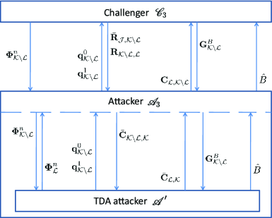
Figure 8: The third constructed experiment for proving Lemma 12

1. Same as step 1) in the first experiment with $\mathscr{A}_{3}$ and $\mathscr{C}_{3}$ taking the roles of $\mathscr{A}_{1}$ and $\mathscr{C}_{1}$, respectively.

2. $\mathscr{A}^{\prime}$ selects $\mathbf{q}_{\mathcal{L}}$, $\mathbf{q}^{0}_{\mathcal{K}\setminus\mathcal{L}}$, and $\mathbf{q}^{1}_{\mathcal{K}\setminus\mathcal{L}}$ as in step 2) of the TDA experiment, and then passes $[\mathbf{q}^{0}_{\mathcal{K}\setminus\mathcal{L}},\mathbf{q}^{1}_{\mathcal{K}\setminus\mathcal{L}}]$ to $\mathscr{A}_{3}$, who then passes them on to $\mathscr{C}_{3}$.

3. $\mathscr{C}_{3}$ generates $\mathbf{R}_{\mathcal{K}\setminus\mathcal{L},\mathcal{K}}$ with $\mathbf{R}_{k,l}$ i.i.d. $\sim\mathcal{U}(\mathcal{N}_{m}^{|\mathcal{X}|})$ for $k\neq l$, and $\mathbf{R}_{k,k}=\ominus\bigoplus_{l\in\mathcal{K}\setminus k}\mathbf{R}_{k,l}$ according to (10), and then gives $[{\mathbf{\bar{R}}}_{\mathcal{J},\mathcal{K}\setminus\mathcal{L}},\mathbf{R}_{\mathcal{K}\setminus\mathcal{L},\mathcal{L}}]$ to $\mathscr{A}_{3}$.

4. $\mathscr{A}_{3}$ computes ${\mathbf{\bar{C}}}_{\mathcal{I},\mathcal{K}\setminus\mathcal{L}}=E(0^{2(K-L-1)|\mathcal{X}|};\boldsymbol{\Phi}^{n}_{\mathcal{K}\setminus\mathcal{L}})$, ${\mathbf{\bar{C}}}_{\mathcal{J},\mathcal{K}\setminus\mathcal{L}}=E(\bar{\mathbf{R}}_{\mathcal{J},\mathcal{K}\setminus\mathcal{L}};\boldsymbol{\Phi}^{n}_{\mathcal{K}\setminus\mathcal{L}})$, $\mathbf{C}_{\mathcal{K}\setminus\mathcal{L},\mathcal{L}}=E(\mathbf{R}_{\mathcal{K}\setminus\mathcal{L},\mathcal{L}};\boldsymbol{\Phi}^{n}_{\mathcal{L}})$, and gives ${\mathbf{\bar{C}}}_{\mathcal{K}\setminus\mathcal{L},\mathcal{K}}$ to $\mathscr{A}^{\prime}$.

5. $\mathscr{A}^{\prime}$ follows step 4) of the TDA experiment to decrypt $\mathbf{C}_{\mathcal{K}\setminus\mathcal{L},\mathcal{L}}$, generate $\mathbf{R}_{\mathcal{L},\mathcal{K}}$, encrypt to obtain $\mathbf{\bar{C}}_{\mathcal{L},\mathcal{K}}$, and send $\mathbf{\bar{C}}_{\mathcal{L},\mathcal{K}}$ to $\mathscr{A}_{3}$, who then passes on $\mathbf{C}_{\mathcal{L},\mathcal{K}\setminus\mathcal{L}}$ to $\mathscr{C}_{3}$.

6. $\mathscr{C}_{3}$ calculates $\mathbf{R}_{\mathcal{L},\mathcal{K}\setminus\mathcal{L}}=D(\mathbf{C}_{\mathcal{L},\mathcal{K}\setminus\mathcal{L}};\mathbf{\Psi}^{n}_{\mathcal{K}\setminus\mathcal{L}})$. Then, $\mathscr{C}_{3}$ selects an independent bit $B\in\{0,1\}$ with equal probabilities, computes $\mathbf{G}^{B}_{\mathcal{K}\setminus\mathcal{L}}=\mathbf{q}^{B}_{\mathcal{K}\setminus\mathcal{L}}\oplus\mathbf{\Sigma}_{\mathbf{R}_{\mathcal{K},\mathcal{K}\setminus\mathcal{L}}}$, and gives $\mathbf{G}^{B}_{\mathcal{K}\setminus\mathcal{L}}$ to $\mathscr{A}_{3}$, who passes it on to $\mathscr{A}^{\prime}$.

7. $\mathscr{A}^{\prime}$ uses $\hat{B}=\hat{B}(\mathbf{q}^{0}_{\mathcal{K}\setminus\mathcal{L}},\mathbf{q}^{1}_{\mathcal{K}\setminus\mathcal{L}},\mathbf{q}_{\mathcal{L}},{\mathbf{\bar{C}}}_{\mathcal{K},\mathcal{K}},\mathbf{G}^{B}_{\mathcal{K}\setminus\mathcal{L}},\mathbf{R}_{\mathcal{L},\mathcal{K}},\\ \mathbf{R}_{\mathcal{K}\setminus\mathcal{L},\mathcal{L}},\boldsymbol{\Phi}^{n}_{\mathcal{K}},\boldsymbol{\Psi}^{n}_{\mathcal{L}})$ in step 6) of the TDA experiment with the input arguments as specified to estimate $B$, and reports $\hat{B}$ to $\mathscr{A}_{3}$, who then passes it on to $\mathscr{C}_{3}$.

We will again use Lemmas 9 and 10 by letting $Y=\mathbf{G}^{B}_{\mathcal{K}\setminus\mathcal{L}}$, $U={\mathbf{\bar{R}}}_{\mathcal{J},\mathcal{K}\setminus\mathcal{L}}$, $V=[\mathbf{Q}^{0}_{\mathcal{K}\setminus\mathcal{L}},\mathbf{Q}^{1}_{\mathcal{K}\setminus\mathcal{L}},\mathbf{R}_{\mathcal{L},\mathcal{K}\setminus\mathcal{L}},\mathbf{R}_{\mathcal{K}\setminus\mathcal{L},\mathcal{L}},\boldsymbol{\Phi}^{n}_{\mathcal{K}\setminus\mathcal{L}}]$, $Z_{1}=[\mathbf{Q}_{\mathcal{L}},{\mathbf{\bar{C}}}_{\mathcal{K}\setminus\mathcal{L},\mathcal{K}},\boldsymbol{\Phi}^{n}_{\mathcal{L}},\boldsymbol{\Psi}^{n}_{\mathcal{L}}]$, $Z_{2}=[Y,U,V]$, and $W=[{\mathbf{\bar{C}}}_{\mathcal{L},\mathcal{K}},{\mathbf{R}}_{\mathcal{L},\mathcal{L}},Z_{1}]$ this time. Like before, it is easy to check that we again have $W$ as a PPT function of $[Z_{1},Z_{2}]$ in this case. Thus, we may apply Lemma 10 again to obtain that $W$ is conditionally independent of $B$ given $Z_{2}$ as long as $Z_{1}$ and $B$ are conditionally independent given $Z_{2}$. This latter fact is established by (29), where the equality is based on Assumption 4, (16), and the fact that ${\mathbf{\bar{C}}}_{\mathcal{I},\mathcal{K}\setminus\mathcal{L}}=E(0^{2(K-L-1)|\mathcal{X}|};\boldsymbol{\Phi}^{n}_{\mathcal{K}\setminus\mathcal{L}})$.

$$p_{\mathbf{Q}_{\mathcal{L}},{\mathbf{\bar{C}}}_{\mathcal{K}\setminus\mathcal{L},\mathcal{K}},\boldsymbol{\Phi}^{n}_{\mathcal{L}},\boldsymbol{\Psi}^{n}_{\mathcal{L}}\mid\mathbf{G}^{B}_{\mathcal{K}\setminus\mathcal{L}},{\mathbf{\bar{R}}}_{{\mathcal{J}},\mathcal{K}\setminus\mathcal{L}},\mathbf{Q}^{0}_{\mathcal{K}\setminus\mathcal{L}},\mathbf{Q}^{1}_{\mathcal{K}\setminus\mathcal{L}},{\mathbf{\bar{R}}}_{\mathcal{L},\mathcal{K}\setminus\mathcal{L}},\mathbf{R}_{\mathcal{K}\setminus\mathcal{L},\mathcal{L}},\boldsymbol{\Phi}^{n}_{\mathcal{K}\setminus\mathcal{L}},B}(\mathbf{q}^{\prime}_{\mathcal{L}},{\mathbf{\bar{c}}}_{\mathcal{K}\setminus\mathcal{L},\mathcal{K}},\boldsymbol{\phi}^{n}_{\mathcal{L}},\boldsymbol{\psi}^{n}_{\mathcal{L}}\mid\mathbf{g}_{\mathcal{K}\setminus\mathcal{L}},{\mathbf{\bar{r}}}_{{\mathcal{J}},\mathcal{K}\setminus\mathcal{L}},\mathbf{q}^{\prime}_{\mathcal{K}\setminus\mathcal{L}},\mathbf{q}^{\prime\prime}_{\mathcal{K}\setminus\mathcal{L}},{\mathbf{\bar{r}}}_{\mathcal{L},\mathcal{K}\setminus\mathcal{L}},$$

$$\hskip 20.0pt\mathbf{r}_{\mathcal{K}\setminus\mathcal{L},\mathcal{L}},\boldsymbol{\phi}^{n}_{\mathcal{K}\setminus\mathcal{L}},b)$$

$$=\delta_{\mathbf{q}_{\mathcal{L}}}(\mathbf{q}^{\prime}_{\mathcal{L}})\cdot p_{{\mathbf{\bar{C}}}_{\mathcal{J},\mathcal{K}\setminus\mathcal{L}}\mid{\mathbf{\bar{R}}}_{\mathcal{J},\mathcal{K}\setminus\mathcal{L}},\boldsymbol{\Phi}^{n}_{\mathcal{K}\setminus\mathcal{L}}}(\mathbf{\bar{c}}_{\mathcal{J},\mathcal{K}\setminus\mathcal{L}}\mid{\mathbf{\bar{r}}}_{\mathcal{J},\mathcal{K}\setminus\mathcal{L}},\boldsymbol{\phi}^{n}_{\mathcal{K}\setminus\mathcal{L}})\cdot p_{{\mathbf{C}}_{\mathcal{K}\setminus\mathcal{L},\mathcal{L}}\mid\mathbf{R}_{\mathcal{K}\setminus\mathcal{L},\mathcal{L}},\boldsymbol{\Phi}^{n}_{\mathcal{L}}}({\mathbf{c}}_{\mathcal{K}\setminus\mathcal{L},\mathcal{L}}\mid\mathbf{r}_{\mathcal{K}\setminus\mathcal{L},\mathcal{L}},\boldsymbol{\phi}^{n}_{\mathcal{L}})$$

$$\hskip 20.0pt\cdot p_{{\mathbf{\bar{C}}}_{\mathcal{I},\mathcal{K}\setminus\mathcal{L}}\mid\boldsymbol{\Phi}^{n}_{\mathcal{K}\setminus\mathcal{L}}}(\mathbf{\bar{c}}_{\mathcal{I},\mathcal{K}\setminus\mathcal{L}}\mid\boldsymbol{\phi}^{n}_{\mathcal{K}\setminus\mathcal{L}})\cdot p_{\boldsymbol{\Phi}^{n}_{\mathcal{L}},\boldsymbol{\Psi}^{n}_{\mathcal{L}}\mid\boldsymbol{\Phi}^{n}_{\mathcal{K}\setminus\mathcal{L}}}(\boldsymbol{\phi}^{n}_{\mathcal{L}},\boldsymbol{\psi}^{n}_{\mathcal{L}}\mid\boldsymbol{\phi}^{n}_{\mathcal{K}\setminus\mathcal{L}})$$ (29)

Further, expressed in the previous notation $\hat{B}(Y,V,W)=\hat{B}(\boldsymbol{\Xi},\boldsymbol{\Gamma}_{1},\mathbf{G}^{B}_{\mathcal{K}\setminus\mathcal{L}})$. Thus, by applying Lemma 9 with $Y$, $U$, $V$, and $W$ as specified, we get a reduced PPT estimator $\hat{B}_{3}(\mathbf{G}^{B}_{\mathcal{K}\setminus\mathcal{L}},\mathbf{Q}^{0}_{\mathcal{K}\setminus\mathcal{L}},\mathbf{Q}^{1}_{\mathcal{K}\setminus\mathcal{L}},{\mathbf{\bar{R}}}_{\mathcal{K}\setminus\mathcal{I},\mathcal{K}\setminus\mathcal{L}},\mathbf{R}_{\mathcal{K}\setminus\mathcal{L},\mathcal{L}},\boldsymbol{\Phi}^{n}_{\mathcal{K}\setminus\mathcal{L}})$ that satisfies

$$\Pr(\hat{B}(\boldsymbol{\Xi},\boldsymbol{\Gamma}_{1},\mathbf{G}^{B}_{\mathcal{K}\setminus\mathcal{L}})=B\mid\mathbb{Q}(\mathbf{q}^{0}_{\mathcal{K}\setminus\mathcal{L}},\mathbf{q}^{1}_{\mathcal{K}\setminus\mathcal{L}},\mathbf{q}_{\mathcal{L}}),$$

$$\hskip 10.0pt\mathbf{\bar{R}}_{\mathcal{K}\setminus\mathcal{I},\mathcal{K}\setminus\mathcal{L}}=\mathbf{\bar{r}}_{\mathcal{K}\setminus\mathcal{I},\mathcal{K}\setminus\mathcal{L}},\mathbf{R}_{\mathcal{K}\setminus\mathcal{L},\mathcal{L}}=\mathbf{r}_{\mathcal{K}\setminus\mathcal{L},\mathcal{L}},\boldsymbol{\Phi}^{n}_{\mathcal{K}\setminus\mathcal{L}}=\boldsymbol{\phi}^{n}_{\mathcal{K}\setminus\mathcal{L}})$$

$$=\Pr(\hat{B}_{3}=B\mid\mathbb{Q}(\mathbf{q}^{0}_{\mathcal{K}\setminus\mathcal{L}},\mathbf{q}^{1}_{\mathcal{K}\setminus\mathcal{L}},\mathbf{q}_{\mathcal{L}}),\mathbf{\bar{R}}_{\mathcal{K}\setminus\mathcal{I},\mathcal{K}\setminus\mathcal{L}}=\mathbf{\bar{r}}_{\mathcal{K}\setminus\mathcal{I},\mathcal{K}\setminus\mathcal{L}},$$

$$\hskip 30.0pt\mathbf{R}_{\mathcal{K}\setminus\mathcal{L},\mathcal{L}}=\mathbf{r}_{\mathcal{K}\setminus\mathcal{L},\mathcal{L}},\boldsymbol{\Phi}^{n}_{\mathcal{K}\setminus\mathcal{L}}=\boldsymbol{\phi}^{n}_{\mathcal{K}\setminus\mathcal{L}})$$

$$=\frac{1}{2}$$ (30)

where we have used the triviality of the distribution of $\mathbf{Q}_{\mathcal{L}}$ in the first equality, and the last equality can be obtained based on Lemma 8 as shown in Appendix C.

Since both $\hat{B}(\boldsymbol{\Xi},\boldsymbol{\Gamma}_{1},\mathbf{G}^{0}_{\mathcal{K}\setminus\mathcal{L}})$ and $\hat{B}(\boldsymbol{\Xi},\boldsymbol{\Gamma}_{1},\mathbf{G}^{1}_{\mathcal{K}\setminus\mathcal{L}})$ are conditionally independent of $B$ given $[\mathbf{Q}^{0}_{\mathcal{K}\setminus\mathcal{L}},\mathbf{Q}^{1}_{\mathcal{K}\setminus\mathcal{L}},\mathbf{Q}_{\mathcal{L}}]$, (30) implies

$$\frac{1}{2}\Pr(\hat{B}(\boldsymbol{\Xi},\boldsymbol{\Gamma}_{1},\mathbf{G}^{0}_{\mathcal{K}\setminus\mathcal{L}})=0\mid\mathbb{Q}(\mathbf{q}^{0}_{\mathcal{K}\setminus\mathcal{L}},\mathbf{q}^{1}_{\mathcal{K}\setminus\mathcal{L}},\mathbf{q}_{\mathcal{L}}))$$

$$+\frac{1}{2}\Pr(\hat{B}(\boldsymbol{\Xi},\boldsymbol{\Gamma}_{1},\mathbf{G}^{1}_{\mathcal{K}\setminus\mathcal{L}})=1\mid\mathbb{Q}(\mathbf{q}^{0}_{\mathcal{K}\setminus\mathcal{L}},\mathbf{q}^{1}_{\mathcal{K}\setminus\mathcal{L}},\mathbf{q}_{\mathcal{L}}))$$

$$=\frac{1}{2}.$$ (31)

Finally, adding up (27), (28), and (31) from the three experiments constructed above gives

$$\Pr(\hat{B}(\boldsymbol{\Xi},\boldsymbol{\Gamma}_{0},\mathbf{G}^{B}_{\mathcal{K}\setminus\mathcal{L}})=B\mid\mathbb{Q}(\mathbf{q}^{0}_{\mathcal{K}\setminus\mathcal{L}},\mathbf{q}^{1}_{\mathcal{K}\setminus\mathcal{L}},\mathbf{q}_{\mathcal{L}}))$$

$$=\frac{1}{2}\Pr(\hat{B}(\boldsymbol{\Xi},\boldsymbol{\Gamma}_{0},\mathbf{G}^{0}_{\mathcal{K}\setminus\mathcal{L}})=0\mid\mathbb{Q}(\mathbf{q}^{0}_{\mathcal{K}\setminus\mathcal{L}},\mathbf{q}^{1}_{\mathcal{K}\setminus\mathcal{L}},\mathbf{q}_{\mathcal{L}}))$$

$$+\frac{1}{2}\Pr(\hat{B}(\boldsymbol{\Xi},\boldsymbol{\Gamma}_{0},\mathbf{G}^{1}_{\mathcal{K}\setminus\mathcal{L}})=1\mid\mathbb{Q}(\mathbf{q}^{0}_{\mathcal{K}\setminus\mathcal{L}},\mathbf{q}^{1}_{\mathcal{K}\setminus\mathcal{L}},\mathbf{q}_{\mathcal{L}}))$$

$$\leq\frac{1}{2}+4(K-L-1)|\mathcal{X}|\cdot F_{\mathrm{CPA}}(n).$$ (32)

Note that $\hat{B}(\boldsymbol{\Xi},\boldsymbol{\Gamma}_{0},\mathbf{G}^{B}_{\mathcal{K}\setminus\mathcal{L}})$ is exactly the estimator $\hat{B}$ used by $\mathscr{A}^{\prime}$ in step 6) of the TDA experiment. As a result, (32) establishes (23). ∎

V-E Proof of Theorem 7

As discussed before, we will reduce the TEA experiment to a TDA experiment by constructing a TDA attacker $\mathscr{A}^{\prime}$ and her estimator $\hat{B}$ (see step 6) of the TDA experiment from the TEA attacker $\mathscr{A}$ and her estimator $\mathbf{\hat{Q}}_{\mathcal{K}\setminus\mathcal{L}}$ (see (18)). This reduction allows us to express the winning probability of $\mathscr{A}$ as that of $\mathscr{A}^{\prime}$, thus proving (19) using Lemma 12. The steps of the constructed TDA experiment, shown in Figure 9, are as follows:

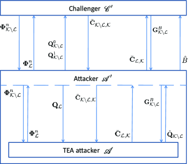
Figure 9: The constructed experiment for proving Theorem 7

1. $\mathscr{C}^{\prime}$ runs $S(1^{n})$ to get the key pair collection $(\boldsymbol{\Phi}^{n}_{\mathcal{K}\setminus\mathcal{L}},\boldsymbol{\Psi}^{n}_{\mathcal{K}\setminus\mathcal{L}})$ and gives $\boldsymbol{\Phi}^{n}_{\mathcal{K}\setminus\mathcal{L}}$ to $\mathscr{A}^{\prime}$, who passes it on to $\mathscr{A}$. Then, $\mathscr{A}$ generates the key pair collection $(\boldsymbol{\Phi}_{\mathcal{L}}^{n},\boldsymbol{\Psi}_{\mathcal{L}}^{n})$ according to (16) and gives $\boldsymbol{\Phi}_{\mathcal{L}}^{n}$ to $\mathscr{A}^{\prime}$, who then passes it on to $\mathscr{C}^{\prime}$.

2. $\mathscr{A}^{\prime}$ draws $[\mathbf{Q}^{0}_{\mathcal{K}\setminus\mathcal{L}},\mathbf{Q}_{\mathcal{L}}]\in\mathcal{Q}_{t}^{K}(\mathcal{X})$ according to $p_{\mathbf{Q}_{\mathcal{K}}}$ and $\mathbf{Q}^{1}_{\mathcal{K}\setminus\mathcal{L}}\in\mathcal{Q}_{t}^{K-L}(\mathcal{X})$ according to $p_{\mathbf{Q}_{\mathcal{K}\setminus\mathcal{L}}\mid\boldsymbol{\Sigma}_{\mathbf{Q}_{\mathcal{K}\setminus\mathcal{L}}},\mathbf{Q}_{\mathcal{L}}}(\cdot\mid\boldsymbol{\Sigma}_{\mathbf{Q}^{0}_{\mathcal{K}\setminus\mathcal{L}}},\mathbf{Q}_{\mathcal{L}})$. Then, $\mathscr{A}^{\prime}$ gives $[\mathbf{Q}^{0}_{\mathcal{K}\setminus\mathcal{L}},\mathbf{Q}^{1}_{\mathcal{K}\setminus\mathcal{L}}]$ to $\mathscr{C}^{\prime}$ and $\mathbf{Q}_{\mathcal{L}}$ to $\mathscr{A}$.

3. Same as step 3) of the TDA experiment. Then $\mathscr{A}^{\prime}$ passes $\mathbf{\bar{C}}_{\mathcal{K}\setminus\mathcal{L},\mathcal{K}}$ to $\mathscr{A}$.

4. $\mathscr{A}$ follows step 4) of the TEA experiment to calculate $\mathbf{R}_{\mathcal{K}\setminus\mathcal{L},\mathcal{L}}$, $\mathbf{R}_{\mathcal{L},\mathcal{K}}$, and ${\mathbf{\bar{C}}}_{\mathcal{L},\mathcal{K}}$. Then, she gives ${\mathbf{\bar{C}}}_{\mathcal{L},\mathcal{K}}$ to $\mathscr{A}^{\prime}$, who passes it on to $\mathscr{C}^{\prime}$.

5. Same as step 5) of the TDA experiment. Then, $\mathscr{A}^{\prime}$ passes $\mathbf{G}^{B}_{\mathcal{K}\setminus\mathcal{L}}$ on to $\mathscr{A}$.

6. $\mathscr{A}$ follows step 6) of the TEA experiment to compute $\mathbf{G}_{\mathcal{L}}$ and reports her estimate ${\mathbf{\hat{Q}}}_{\mathcal{K}\setminus\mathcal{L}}=\mathbf{\hat{Q}}_{\mathcal{K}\setminus\mathcal{L}}(\mathbf{Q}_{\mathcal{L}},\mathbf{\Phi}^{n}_{\mathcal{K}},\\ \mathbf{\Psi}^{n}_{\mathcal{L}},\mathbf{\bar{C}}_{\mathcal{K},\mathcal{K}},[\mathbf{G}^{B}_{\mathcal{K}\setminus\mathcal{L}},\mathbf{G}_{\mathcal{L}}],\mathbf{R}_{\mathcal{L},\mathcal{K}},\mathbf{R}_{\mathcal{K}\setminus\mathcal{L},\mathcal{L}})$ to $\mathscr{A}^{\prime}$.

7. Given $\tau\geq 0$, $\mathscr{A}^{\prime}$ estimates $B$ by setting $\hat{B}=0$ if ${\mathbf{\hat{Q}}}_{\mathcal{K}\backslash\mathcal{L}}\in\mathcal{N}_{\tau}(\mathbf{Q}^{0}_{\mathcal{K}\backslash\mathcal{L}})$ and $\hat{B}=1$ otherwise. Then, $\mathscr{A}^{\prime}$ reports $\hat{B}$ to $\mathscr{C}^{\prime}$.

Note that the estimator $\hat{B}=\hat{B}(\mathbf{Q}^{0}_{\mathcal{K}\setminus\mathcal{L}},\mathbf{Q}^{1}_{\mathcal{K}\setminus\mathcal{L}},\mathbf{Q}_{\mathcal{L}},{\mathbf{\bar{C}}}_{\mathcal{K},\mathcal{K}},\mathbf{G}_{\mathcal{L}},\\ \mathbf{G}^{B}_{\mathcal{K}\setminus\mathcal{L}},\mathbf{R}_{\mathcal{L},\mathcal{K}},\mathbf{R}_{\mathcal{K}\setminus\mathcal{L},\mathcal{L}},\boldsymbol{\Phi}^{n}_{\mathcal{K}},\boldsymbol{\Psi}^{n}_{\mathcal{L}})$ because of the functional form of ${\mathbf{\hat{Q}}}_{\mathcal{K}\backslash\mathcal{L}}$ (see (18)).

We will use Lemma 9 by setting $Y=[{\mathbf{\bar{C}}}_{\mathcal{K},\mathcal{K}},\mathbf{G}^{B}_{\mathcal{K}\setminus\mathcal{L}},\mathbf{R}_{\mathcal{L},\mathcal{K}},\\ \mathbf{R}_{\mathcal{K}\setminus\mathcal{L},\mathcal{L}},\boldsymbol{\Phi}^{n}_{\mathcal{K}},\boldsymbol{\Psi}^{n}_{\mathcal{L}}]$, $U=\emptyset$, $V=[\mathbf{Q}^{0}_{\mathcal{K}\setminus\mathcal{L}},\mathbf{Q}^{1}_{\mathcal{K}\setminus\mathcal{L}},\mathbf{Q}_{\mathcal{L}}]$, and $W=\mathbf{G}_{\mathcal{L}}$. Since $\mathbf{G}_{\mathcal{L}}=\mathbf{Q}_{\mathcal{L}}\oplus\boldsymbol{\Sigma}_{\mathbf{R}_{\mathcal{K},\mathcal{L}}}$ and $\boldsymbol{\Sigma}_{\mathbf{R}_{\mathcal{K},\mathcal{L}}}$ is a deterministic function of $[\mathbf{R}_{\mathcal{L},\mathcal{K}},\mathbf{R}_{\mathcal{K}\setminus\mathcal{L},\mathcal{L}}]$, it is clear that $W$ and $B$ are conditionally independent given $[Y,U,V]$ and the generation of $W$ from $[Y,U,V]$ is PPT. Thus, Lemma 9 applies in this case to give a PPT estimator $\hat{B}_{0}(Y,U,V)$ satisfying

$$\Pr(\hat{B}(Y,V,W)=B\mid\mathbb{Q}(\mathbf{q}^{0}_{\mathcal{K}\setminus\mathcal{L}},\mathbf{q}^{1}_{\mathcal{K}\setminus\mathcal{L}},\mathbf{q}_{\mathcal{L}}))$$

$$=\Pr(\hat{B}_{0}(Y,U,V)=B\mid\mathbb{Q}(\mathbf{q}^{0}_{\mathcal{K}\setminus\mathcal{L}},\mathbf{q}^{1}_{\mathcal{K}\setminus\mathcal{L}},\mathbf{q}_{\mathcal{L}}))$$

$$\leq\frac{1}{2}+4(K-L-1)|\mathcal{X}|\cdot F_{\mathrm{CPA}}(n)$$ (33)

where the last inequality is due to Lemma 12 because the estimator $\hat{B}_{0}(Y,U,V)=\hat{B}_{0}(\mathbf{Q}^{0}_{\mathcal{K}\setminus\mathcal{L}},\mathbf{Q}^{1}_{\mathcal{K}\setminus\mathcal{L}},\mathbf{Q}_{\mathcal{L}},{\mathbf{\bar{C}}}_{\mathcal{K},\mathcal{K}},\mathbf{G}^{B}_{\mathcal{K}\setminus\mathcal{L}},\\ \mathbf{R}_{\mathcal{L},\mathcal{K}},\mathbf{R}_{\mathcal{K}\setminus\mathcal{L},\mathcal{L}},\boldsymbol{\Phi}^{n}_{\mathcal{K}},\boldsymbol{\Psi}^{n}_{\mathcal{L}})$ is exactly in the form of the estimator in step 6) of the TDA experiment.

By the defintion of $\hat{B}$ in step 7) of the constructed TDA experiment, we have

$$\Pr(\hat{B}(Y,V,W)=B\mid\mathbb{Q}(\mathbf{q}^{0}_{\mathcal{K}\setminus\mathcal{L}},\mathbf{q}^{1}_{\mathcal{K}\setminus\mathcal{L}},\mathbf{q}_{\mathcal{L}}))$$

$$=\frac{1}{2}\Pr({\mathbf{\hat{Q}}}_{\mathcal{K}\setminus\mathcal{L}}\in\mathcal{N}_{\tau}(\mathbf{Q}^{0}_{\mathcal{K}\setminus\mathcal{L}})\mid\mathbb{Q}(\mathbf{q}^{0}_{\mathcal{K}\setminus\mathcal{L}},\mathbf{q}^{1}_{\mathcal{K}\setminus\mathcal{L}},\mathbf{q}_{\mathcal{L}}),B=0)$$

$$\hskip 10.0pt+\frac{1}{2}\Big{\{}1-\Pr({\mathbf{\hat{Q}}}_{\mathcal{K}\setminus\mathcal{L}}\in\mathcal{N}_{\tau}(\mathbf{Q}^{0}_{\mathcal{K}\setminus\mathcal{L}})\mid\mathbb{Q}(\mathbf{q}^{0}_{\mathcal{K}\setminus\mathcal{L}},\mathbf{q}^{1}_{\mathcal{K}\setminus\mathcal{L}},\mathbf{q}_{\mathcal{L}}),$$

$$\hskip 75.0ptB=1)\Big{\}}$$ (34)

where we have used the fact that $B$ and $[\mathbf{Q}^{0}_{\mathcal{K}\setminus\mathcal{L}},\mathbf{Q}^{1}_{\mathcal{K}\setminus\mathcal{L}},\mathbf{Q}_{\mathcal{L}}]$ are independent. Putting (34) into (33) gives

$$\Pr({\mathbf{\hat{Q}}}_{\mathcal{K}\setminus\mathcal{L}}\in\mathcal{N}_{\tau}(\mathbf{Q}^{0}_{\mathcal{K}\setminus\mathcal{L}})\mid\mathbb{Q}(\mathbf{q}^{0}_{\mathcal{K}\setminus\mathcal{L}},\mathbf{q}^{1}_{\mathcal{K}\setminus\mathcal{L}},\mathbf{q}_{\mathcal{L}}),B=0)$$

$$\leq\Pr({\mathbf{\hat{Q}}}_{\mathcal{K}\setminus\mathcal{L}}\in\mathcal{N}_{\tau}(\mathbf{Q}^{0}_{\mathcal{K}\setminus\mathcal{L}})\mid\mathbb{Q}(\mathbf{q}^{0}_{\mathcal{K}\setminus\mathcal{L}},\mathbf{q}^{1}_{\mathcal{K}\setminus\mathcal{L}},\mathbf{q}_{\mathcal{L}}),B=1)$$

$$\hskip 10.0pt+8(K-L-1)|\mathcal{X}|\cdot F_{\mathrm{CPA}}(n).$$ (35)

To simply notation, let $\boldsymbol{\Upsilon}=[\mathbf{\Phi}^{n}_{\mathcal{K}},\mathbf{\Psi}^{n}_{\mathcal{L}},\mathbf{\bar{C}}_{\mathcal{K},\mathcal{K}},\mathbf{G}_{\mathcal{L}}$, $\mathbf{R}_{\mathcal{L},\mathcal{K}},\mathbf{R}_{\mathcal{K}\setminus\mathcal{L},\mathcal{L}}]$. Conditioned on $B=0$, $\mathbf{\hat{Q}}_{\mathcal{K}\setminus\mathcal{L}}$ is a function of $\boldsymbol{\Upsilon}$, $\mathbf{Q}_{\mathcal{L}}$, and $\mathbf{G}^{0}_{\mathcal{K}\setminus\mathcal{L}}$. For any $\mathbf{q}^{0}_{\mathcal{K}\setminus\mathcal{L}}$, $\mathbf{q}^{1}_{\mathcal{K}\setminus\mathcal{L}}$, and $\boldsymbol{\sigma}$ satisfying $\boldsymbol{\Sigma}_{\mathbf{q}^{0}_{\mathcal{K}\setminus\mathcal{L}}}=\boldsymbol{\Sigma}_{\mathbf{q}^{1}_{\mathcal{K}\setminus\mathcal{L}}}=\boldsymbol{\sigma}$, we thus have

$$\Pr({\mathbf{\hat{Q}}}_{\mathcal{K}\setminus\mathcal{L}}\in\mathcal{N}_{\tau}(\mathbf{Q}^{0}_{\mathcal{K}\setminus\mathcal{L}})\mid\mathbb{Q}(\mathbf{q}^{0}_{\mathcal{K}\setminus\mathcal{L}},\mathbf{q}^{1}_{\mathcal{K}\setminus\mathcal{L}},\mathbf{q}_{\mathcal{L}}),B=0)$$

$$=\sum_{\boldsymbol{\upsilon},\mathbf{g}_{\mathcal{K}\setminus\mathcal{L}}}\sum_{\mathbf{q}^{\prime}_{\mathcal{K}\setminus\mathcal{L}}\in\mathcal{N}_{\tau}(\mathbf{q}^{0}_{\mathcal{K}\setminus\mathcal{L}})}p_{\mathbf{\hat{Q}}_{\mathcal{K}\setminus\mathcal{L}}\mid\boldsymbol{\Upsilon},\mathbf{Q}_{\mathcal{L}},\mathbf{G}^{0}_{\mathcal{K}\setminus\mathcal{L}}}(\mathbf{q}^{\prime}_{\mathcal{K}\setminus\mathcal{L}}\mid\boldsymbol{\upsilon},\mathbf{q}_{\mathcal{L}},\mathbf{g}_{\mathcal{K}\setminus\mathcal{L}})\cdot$$

$$\hskip 30.0ptp_{\boldsymbol{\Upsilon},\mathbf{G}^{0}_{\mathcal{K}\setminus\mathcal{L}}\mid\mathbf{Q}^{0}_{\mathcal{K}\setminus\mathcal{L}},\mathbf{Q}^{1}_{\mathcal{K}\setminus\mathcal{L}},\mathbf{Q}_{\mathcal{L}}}(\boldsymbol{\upsilon},\mathbf{g}_{\mathcal{K}\setminus\mathcal{L}}\mid\mathbf{q}^{0}_{\mathcal{K}\setminus\mathcal{L}},\mathbf{q}^{1}_{\mathcal{K}\setminus\mathcal{L}},\mathbf{q}_{\mathcal{L}})$$

$$=\sum_{\boldsymbol{\upsilon},\mathbf{g}_{\mathcal{K}\setminus\mathcal{L}}}\sum_{\mathbf{q}^{\prime}_{\mathcal{K}\setminus\mathcal{L}}\in\mathcal{N}_{\tau}(\mathbf{q}^{0}_{\mathcal{K}\setminus\mathcal{L}})}p_{\mathbf{\hat{Q}}_{\mathcal{K}\setminus\mathcal{L}}\mid\boldsymbol{\Upsilon},\mathbf{Q}_{\mathcal{L}},\mathbf{G}^{0}_{\mathcal{K}\setminus\mathcal{L}}}(\mathbf{q}^{\prime}_{\mathcal{K}\setminus\mathcal{L}}\mid\boldsymbol{\upsilon},\mathbf{q}_{\mathcal{L}},\mathbf{g}_{\mathcal{K}\setminus\mathcal{L}})\cdot$$

$$p_{\boldsymbol{\Upsilon},\mathbf{G}^{0}_{\mathcal{K}\setminus\mathcal{L}}\mid\mathbf{Q}^{0}_{\mathcal{K}\setminus\mathcal{L}},\mathbf{Q}^{1}_{\mathcal{K}\setminus\mathcal{L}},\boldsymbol{\Sigma}_{\mathbf{Q}^{0}_{\mathcal{K}\setminus\mathcal{L}}},\mathbf{Q}_{\mathcal{L}}}(\boldsymbol{\upsilon},\mathbf{g}_{\mathcal{K}\setminus\mathcal{L}}\mid\mathbf{q}^{0}_{\mathcal{K}\setminus\mathcal{L}},\mathbf{q}^{1}_{\mathcal{K}\setminus\mathcal{L}},\boldsymbol{\sigma},\mathbf{q}_{\mathcal{L}})$$

$$=\Pr({\mathbf{\hat{Q}}}_{\mathcal{K}\setminus\mathcal{L}}\in\mathcal{N}_{\tau}(\mathbf{q}^{0}_{\mathcal{K}\setminus\mathcal{L}})\mid\mathbf{Q}_{\mathcal{K}\setminus\mathcal{L}}=\mathbf{q}^{0}_{\mathcal{K}\setminus\mathcal{L}},\mathbf{Q}^{1}_{\mathcal{K}\setminus\mathcal{L}}=\mathbf{q}^{1}_{\mathcal{K}\setminus\mathcal{L}},$$

$$\hskip 40.0pt\boldsymbol{\Sigma}_{\mathbf{Q}_{\mathcal{K}\setminus\mathcal{L}}}=\boldsymbol{\sigma},\mathbf{Q}_{\mathcal{L}}=\mathbf{q}_{\mathcal{L}})$$ (36)

where the first equality results because $B$ is independent of $[\boldsymbol{\Upsilon},\mathbf{G}^{0}_{\mathcal{K}\setminus\mathcal{L}},\mathbf{Q}^{0}_{\mathcal{K}\setminus\mathcal{L}},\mathbf{Q}^{1}_{\mathcal{K}\setminus\mathcal{L}},\mathbf{Q}_{\mathcal{L}}]$, the second equality is due to the fact that $\boldsymbol{\Sigma}_{\mathbf{Q}^{0}_{\mathcal{K}\setminus\mathcal{L}}}$ is a deterministic function of $\mathbf{Q}^{0}_{\mathcal{K}\setminus\mathcal{L}}$, and the last equality is simply re-identifying $\mathbf{G}^{0}_{\mathcal{K}\setminus\mathcal{L}}$ as $\mathbf{G}_{\mathcal{K}\setminus\mathcal{L}}$ and $\mathbf{Q}^{0}_{\mathcal{K}\setminus\mathcal{L}}$ as $\mathbf{Q}_{\mathcal{K}\setminus\mathcal{L}}$ to fit the description in the TEA experiment because $\mathbf{Q}^{0}_{\mathcal{K}\setminus\mathcal{L}}$ (resp. $\mathbf{G}^{0}_{\mathcal{K}\setminus\mathcal{L}}$) has the same conditional distribution as that of $\mathbf{Q}_{\mathcal{K}\setminus\mathcal{L}}$ (resp. $\mathbf{G}_{\mathcal{K}\setminus\mathcal{L}}$) given $[\boldsymbol{\Sigma}_{\mathbf{Q}_{\mathcal{K}\setminus\mathcal{L}}},\mathbf{Q}_{\mathcal{L}}]$. We will write $\mathbf{Q}_{\mathcal{K}\setminus\mathcal{L}}$ (resp. $\mathbf{G}_{\mathcal{K}\setminus\mathcal{L}}$) instead of $\mathbf{Q}^{0}_{\mathcal{K}\setminus\mathcal{L}}$ (resp. $\mathbf{G}^{0}_{\mathcal{K}\setminus\mathcal{L}}$) below for matching the notation in Theorem 7.

Conditioned on $B=1$, $\mathbf{\hat{Q}}_{\mathcal{K}\setminus\mathcal{L}}$ is a function of $\boldsymbol{\Upsilon}$, $\mathbf{Q}_{\mathcal{L}}$, and $\mathbf{G}^{1}_{\mathcal{K}\setminus\mathcal{L}}$ instead. To distinguish from $\mathbf{\hat{Q}}_{\mathcal{K}\setminus\mathcal{L}}=\mathbf{\hat{Q}}_{\mathcal{K}\setminus\mathcal{L}}(\boldsymbol{\Upsilon},\mathbf{Q}_{\mathcal{L}},\mathbf{G}^{0}_{\mathcal{K}\setminus\mathcal{L}})$, let $\mathbf{\hat{Q}}^{\prime}_{\mathcal{K}\setminus\mathcal{L}}=\mathbf{\hat{Q}}_{\mathcal{K}\setminus\mathcal{L}}(\boldsymbol{\Upsilon},\mathbf{Q}_{\mathcal{L}},\mathbf{G}^{1}_{\mathcal{K}\setminus\mathcal{L}})$ in this case. A similar argument as above follows to show that

$$\Pr({\mathbf{\hat{Q}}}_{\mathcal{K}\setminus\mathcal{L}}\in\mathcal{N}_{\tau}(\mathbf{Q}^{0}_{\mathcal{K}\setminus\mathcal{L}})\mid\mathbb{Q}(\mathbf{q}^{0}_{\mathcal{K}\setminus\mathcal{L}},\mathbf{q}^{1}_{\mathcal{K}\setminus\mathcal{L}},\mathbf{q}_{\mathcal{L}}),B=1)$$

$$=\Pr(\mathbf{\hat{Q}}^{\prime}_{\mathcal{K}\setminus\mathcal{L}}\in\mathcal{N}_{\tau}(\mathbf{q}^{0}_{\mathcal{K}\setminus\mathcal{L}})\mid\mathbf{Q}_{\mathcal{K}\setminus\mathcal{L}}=\mathbf{q}^{0}_{\mathcal{K}\setminus\mathcal{L}},\mathbf{Q}^{1}_{\mathcal{K}\setminus\mathcal{L}}=\mathbf{q}^{1}_{\mathcal{K}\setminus\mathcal{L}},$$

$$\hskip 40.0pt\boldsymbol{\Sigma}_{\mathbf{Q}_{\mathcal{K}\setminus\mathcal{L}}}=\boldsymbol{\sigma},\mathbf{Q}_{\mathcal{L}}=\mathbf{q}_{\mathcal{L}}).$$ (37)

Applying (36) and (37) to (35), and then conditionally averaging with respect to $[\mathbf{Q}_{\mathcal{K}\setminus\mathcal{L}},\mathbf{Q}^{1}_{\mathcal{K}\setminus\mathcal{L}}]$ gives (19).

The conditional independence between $\mathbf{\hat{Q}}^{\prime}_{\mathcal{K}\setminus\mathcal{L}}$ and $\mathbf{Q}_{\mathcal{K}\setminus\mathcal{L}}$ given $[\boldsymbol{\Sigma}_{\mathbf{Q}_{\mathcal{K}\setminus\mathcal{L}}},\mathbf{Q}_{\mathcal{L}}]$ follows from

$$p_{\mathbf{\hat{Q}}^{\prime}_{\mathcal{K}\setminus\mathcal{L}}\mid\mathbf{Q}_{\mathcal{K}\setminus\mathcal{L}},\boldsymbol{\Sigma}_{\mathbf{Q}_{\mathcal{K}\setminus\mathcal{L}}},\mathbf{Q}_{\mathcal{L}}}(\mathbf{q}^{\prime}_{\mathcal{K}\setminus\mathcal{L}}\mid\mathbf{q}_{\mathcal{K}\setminus\mathcal{L}},\boldsymbol{\sigma},\mathbf{q}_{\mathcal{L}})$$

$$=\sum_{\boldsymbol{\upsilon},\mathbf{g}_{\mathcal{K}\setminus\mathcal{L}}}\sum_{\mathbf{q}^{1}_{\mathcal{K}\setminus\mathcal{L}}:\boldsymbol{\Sigma}_{\mathbf{q}^{1}_{\mathcal{K}\setminus\mathcal{L}}}=\boldsymbol{\sigma}}p_{\mathbf{\hat{Q}}^{\prime}_{\mathcal{K}\setminus\mathcal{L}}\mid\boldsymbol{\Upsilon},\mathbf{Q}_{\mathcal{L}},\mathbf{G}^{1}_{\mathcal{K}\setminus\mathcal{L}}}(\mathbf{q}^{\prime}_{\mathcal{K}\setminus\mathcal{L}}\mid\boldsymbol{\upsilon},\mathbf{q}_{\mathcal{L}},\mathbf{g}_{\mathcal{K}\setminus\mathcal{L}})\cdot$$

$$p_{\boldsymbol{\Upsilon},\mathbf{G}^{1}_{\mathcal{K}\setminus\mathcal{L}},\mathbf{Q}^{1}_{\mathcal{K}\setminus\mathcal{L}}\mid\mathbf{Q}_{\mathcal{K}\setminus\mathcal{L}},\boldsymbol{\Sigma}_{\mathbf{Q}_{\mathcal{K}\setminus\mathcal{L}}},\mathbf{Q}_{\mathcal{L}}}(\boldsymbol{\upsilon},\mathbf{g}_{\mathcal{K}\setminus\mathcal{L}},\mathbf{q}^{1}_{\mathcal{K}\setminus\mathcal{L}}\mid\mathbf{q}_{\mathcal{K}\setminus\mathcal{L}},\boldsymbol{\sigma},\mathbf{q}_{\mathcal{L}})$$

$$=\sum_{\boldsymbol{\upsilon},\mathbf{g}_{\mathcal{K}\setminus\mathcal{L}}}p_{\mathbf{\hat{Q}}^{\prime}_{\mathcal{K}\setminus\mathcal{L}}\mid\boldsymbol{\Upsilon},\mathbf{Q}_{\mathcal{L}},\mathbf{G}^{1}_{\mathcal{K}\setminus\mathcal{L}}}(\mathbf{q}^{\prime}_{\mathcal{K}\setminus\mathcal{L}}\mid\boldsymbol{\upsilon},\mathbf{q}_{\mathcal{L}},\mathbf{g}_{\mathcal{K}\setminus\mathcal{L}})\cdot$$

$$\sum_{\mathbf{q}^{1}_{\mathcal{K}\setminus\mathcal{L}}:\boldsymbol{\Sigma}_{\mathbf{q}^{1}_{\mathcal{K}\setminus\mathcal{L}}}=\boldsymbol{\sigma}}p_{\boldsymbol{\Upsilon},\mathbf{G}^{1}_{\mathcal{K}\setminus\mathcal{L}}\mid\mathbf{Q}^{1}_{\mathcal{K}\setminus\mathcal{L}},\boldsymbol{\Sigma}_{\mathbf{Q}_{\mathcal{K}\setminus\mathcal{L}}},\mathbf{Q}_{\mathcal{L}}}(\boldsymbol{\upsilon},\mathbf{g}_{\mathcal{K}\setminus\mathcal{L}}\mid\mathbf{q}^{1}_{\mathcal{K}\setminus\mathcal{L}},\boldsymbol{\sigma},\mathbf{q}_{\mathcal{L}})\cdot$$

$$\hskip 30.0ptp_{\mathbf{Q}_{\mathcal{K}\setminus\mathcal{L}}\mid\boldsymbol{\Sigma}_{\mathbf{Q}_{\mathcal{K}\setminus\mathcal{L}}},\mathbf{Q}_{\mathcal{L}}}(\mathbf{q}^{1}_{\mathcal{K}\setminus\mathcal{L}}\mid\boldsymbol{\sigma},\mathbf{q}_{\mathcal{L}})$$

$$=p_{\mathbf{\hat{Q}}^{\prime}_{\mathcal{K}\setminus\mathcal{L}}\mid\boldsymbol{\Sigma}_{\mathbf{Q}_{\mathcal{K}\setminus\mathcal{L}}},\mathbf{Q}_{\mathcal{L}}}(\mathbf{q}^{\prime}_{\mathcal{K}\setminus\mathcal{L}}\mid\boldsymbol{\sigma},\mathbf{q}_{\mathcal{L}})$$ (38)

where the second equality results because $\mathbf{Q}_{\mathcal{K}\setminus\mathcal{L}}$ and $\mathbf{Q}^{1}_{\mathcal{K}\setminus\mathcal{L}}$ have thee same conditional distribution and are conditionally independent given $[\boldsymbol{\Sigma}_{\mathbf{Q}_{\mathcal{K}\setminus\mathcal{L}}},\mathbf{Q}_{\mathcal{L}}]$ (see step 2) of the constructed experiment), and $\mathbf{Q}_{\mathcal{K}\setminus\mathcal{L}}$ and $[\boldsymbol{\Upsilon},\mathbf{G}^{1}_{\mathcal{K}\setminus\mathcal{L}}]$ are conditionally independent given $[\mathbf{Q}^{1}_{\mathcal{K}\setminus\mathcal{L}},\mathbf{Q}_{\mathcal{K}\setminus\mathcal{L}},\mathbf{Q}_{\mathcal{L}}]$, which in turn is due to that $\mathbf{G}^{1}_{\mathcal{K}\setminus\mathcal{L}}=\mathbf{Q}^{1}_{\mathcal{K}\setminus\mathcal{L}}\oplus\boldsymbol{\Sigma}_{\mathbf{R}_{\mathcal{K},\mathcal{K}\setminus\mathcal{L}}}$ and that $\mathbf{R}_{\mathcal{L},\mathcal{K}}$ is a function in the form of (17).

Finally, note that

$$p_{\mathbf{\hat{Q}}_{\mathcal{K}\setminus\mathcal{L}}\mid\boldsymbol{\Sigma}_{\mathbf{Q}_{\mathcal{K}\setminus\mathcal{L}}},\mathbf{Q}_{\mathcal{L}}}(\mathbf{q}^{\prime}_{\mathcal{K}\setminus\mathcal{L}}\mid\boldsymbol{\sigma},\mathbf{q}_{\mathcal{L}})$$

$$=\sum_{\boldsymbol{\upsilon},\mathbf{g}_{\mathcal{K}\setminus\mathcal{L}}}p_{\mathbf{\hat{Q}}_{\mathcal{K}\setminus\mathcal{L}}\mid\boldsymbol{\Upsilon},\mathbf{Q}_{\mathcal{L}},\mathbf{G}_{\mathcal{K}\setminus\mathcal{L}}}(\mathbf{q}^{\prime}_{\mathcal{K}\setminus\mathcal{L}}\mid\boldsymbol{\upsilon},\mathbf{q}_{\mathcal{L}},\mathbf{g}_{\mathcal{K}\setminus\mathcal{L}})\cdot$$

$$\sum_{\mathbf{q}_{\mathcal{K}\setminus\mathcal{L}}:\boldsymbol{\Sigma}_{\mathbf{q}_{\mathcal{K}\setminus\mathcal{L}}}=\boldsymbol{\sigma}}p_{\boldsymbol{\Upsilon},\mathbf{G}_{\mathcal{K}\setminus\mathcal{L}}\mid\mathbf{Q}_{\mathcal{K}\setminus\mathcal{L}},\boldsymbol{\Sigma}_{\mathbf{Q}_{\mathcal{K}\setminus\mathcal{L}}},\mathbf{Q}_{\mathcal{L}}}(\boldsymbol{\upsilon},\mathbf{g}_{\mathcal{K}\setminus\mathcal{L}}\mid\mathbf{q}_{\mathcal{K}\setminus\mathcal{L}},\boldsymbol{\sigma},\mathbf{q}_{\mathcal{L}})\cdot$$

$$\hskip 30.0ptp_{\mathbf{Q}_{\mathcal{K}\setminus\mathcal{L}}\mid\boldsymbol{\Sigma}_{\mathbf{Q}_{\mathcal{K}\setminus\mathcal{L}}},\mathbf{Q}_{\mathcal{L}}}(\mathbf{q}_{\mathcal{K}\setminus\mathcal{L}}\mid\boldsymbol{\sigma},\mathbf{q}_{\mathcal{L}})$$

$$=p_{\mathbf{\hat{Q}}^{\prime}_{\mathcal{K}\setminus\mathcal{L}}\mid\boldsymbol{\Sigma}_{\mathbf{Q}_{\mathcal{K}\setminus\mathcal{L}}},\mathbf{Q}_{\mathcal{L}}}(\mathbf{q}^{\prime}_{\mathcal{K}\setminus\mathcal{L}}\mid\boldsymbol{\sigma},\mathbf{q}_{\mathcal{L}})$$ (39)

where the second equality results by comparing the expression in the line above is the same as that in second equality line of (38) due to the fact that $p_{\boldsymbol{\Upsilon},\mathbf{G}_{\mathcal{K}\setminus\mathcal{L}}\mid\mathbf{Q}_{\mathcal{K}\setminus\mathcal{L}},\boldsymbol{\Sigma}_{\mathbf{Q}_{\mathcal{K}\setminus\mathcal{L}}},\mathbf{Q}_{\mathcal{L}}}=p_{\boldsymbol{\Upsilon},\mathbf{G}^{1}_{\mathcal{K}\setminus\mathcal{L}}\mid\mathbf{Q}^{1}_{\mathcal{K}\setminus\mathcal{L}},\boldsymbol{\Sigma}_{\mathbf{Q}_{\mathcal{K}\setminus\mathcal{L}}},\mathbf{Q}_{\mathcal{L}}}$ and $p_{\mathbf{\hat{Q}}_{\mathcal{K}\setminus\mathcal{L}}\mid\boldsymbol{\Upsilon},\mathbf{Q}_{\mathcal{L}},\mathbf{G}_{\mathcal{K}\setminus\mathcal{L}}}=p_{\mathbf{\hat{Q}}^{\prime}_{\mathcal{K}\setminus\mathcal{L}}\mid\boldsymbol{\Upsilon},\mathbf{Q}_{\mathcal{L}},\mathbf{G}^{1}_{\mathcal{K}\setminus\mathcal{L}}}$ as $\mathbf{G}_{\mathcal{K}\setminus\mathcal{L}}$ (resp. $\mathbf{\hat{Q}}_{\mathcal{K}\setminus\mathcal{L}}$) and $\mathbf{G}^{1}_{\mathcal{K}\setminus\mathcal{L}}$ (resp. $\mathbf{\hat{Q}}^{\prime}_{\mathcal{K}\setminus\mathcal{L}}$) are obtained from the same function with $\mathbf{Q}_{\mathcal{K}\setminus\mathcal{L}}$ (resp. $\mathbf{G}_{\mathcal{K}\setminus\mathcal{L}}$) and $\mathbf{Q}^{1}_{\mathcal{K}\setminus\mathcal{L}}$ (resp. $\mathbf{G}^{1}_{\mathcal{K}\setminus\mathcal{L}}$) as the respective input arguments.

VI Conclusion

In this paper, we develop a privacy-preserving event detection scheme, in which the marginal types of sensors’ measurements are first obfuscated with ZMS random numbers and then sent to the fusion center for the calculation of a diameter-like decision statistic so that privacy of individual sensors’ data can be protected. We present analysis to show that the proposed detection scheme 1) is optimal in the sense that it achieves the best type-I error exponent error when the type-II error rate is required to be negligible, and 2) is secure against any PPT attacker in the sense that the probability advantage of the attacker successfully estimating the sensors’ measured type over independent guessing is negligible.

Appendix A Proof of Theorem 6

Useful properties

We start by noting a number of properties of the functions involved in Theorem 6. We will use these properties in proving the various parts of the theorem below.

First, both $\Delta_{0}(\cdot)$ and $\Delta_{1}(\cdot)$ are bounded continuous functions in $\mathcal{P}(\mathcal{X}^{K})$ due to the continuity of the KL divergence. In addition, both have positive maximum values since $0\leq d_{0}<d_{1}\leq d_{\max}$. Next, both $\alpha_{*}(\cdot)$ and $\gamma_{*}(\cdot)$ are clearly non-decreasing. It is easy to see that $\alpha_{*}(\gamma)=0$ for $0\leq\gamma\leq d_{0}$, and that $0<\alpha_{*}(d_{1})\leq\alpha_{*}(d_{\max})<\infty$ as $0\leq d_{0}<d_{1}\leq d_{\max}$. Because of the continuity of the functions $\Delta_{0}(\cdot)$ and $d(\cdot)$ in $\mathcal{P}(\mathcal{X}^{K})$, it is also easy to check that $\alpha_{*}(\cdot)$ is right-continuous on $[0,d_{\max})$ and is left-continuous on $(0,d_{\max}]$. Similarly, $\beta^{*}(\cdot)$ is non-increasing and is continuous on $(0,\infty)$.

We note that $\alpha_{*}(\gamma_{*}(\alpha))\geq\alpha$ for $\alpha\in[0,\alpha_{*}(d_{\max})]$. Indeed, as a consequence of its right-continuity on $[0,d_{\max})$, $\alpha_{*}(\gamma_{*}(\alpha))\geq\alpha$ as long as $\gamma_{*}(\alpha)<d_{\max}$. On the other hand, if $\gamma_{*}(\alpha)=d_{\max}$, we have $\alpha_{*}(\gamma_{*}(\alpha))=\alpha_{*}(d_{\max})\geq\alpha$ trivially.

In addition, for any $\gamma\in[0,d_{\max}]$, we have $\gamma_{*}(\alpha)\geq\gamma$ if $\alpha>\alpha_{*}(\gamma)$. Indeed, if $\alpha\in(\alpha_{*}(\gamma),\alpha_{*}(d_{\max})]$, we have $\alpha_{*}(\gamma_{*}(\alpha))\geq\alpha>\alpha_{*}(\gamma)$, which in turn gives $\gamma_{*}(\alpha)\geq\gamma$ as $\alpha_{*}(\cdot)$ is non-decreasing. On the other hand, if $\alpha>\alpha_{*}(d_{\max})$, then $\gamma_{*}(\alpha)=d_{\max}\geq\gamma$ trivially.

Proof of (i)

For $\alpha\in[0,\alpha_{*}(d_{\max})]$, $\alpha_{*}(\gamma_{*}(\alpha))\geq\alpha$ implies that $\Delta_{0}(\mathbf{p}_{\mathcal{K}})\geq\alpha$ if $d(\mathbf{p}_{\mathcal{K}})\geq\gamma_{*}(\alpha)$, which is equivalent to that $d(\mathbf{p}_{\mathcal{K}})<\gamma_{*}(\alpha)$ if $\Delta_{0}(\mathbf{p}_{\mathcal{K}})<\alpha$. This latter assertion gives $\beta_{*}(\alpha)\leq\beta^{*}(\alpha)$. On the other hand, for $\alpha>\alpha_{*}(d_{\max})$, $\gamma_{*}(\alpha)=d_{\max}$, which implies $\beta_{*}(\alpha)=0$. Hence, we have $\beta_{*}(\alpha)\leq\beta^{*}(\alpha)$ trivially.

Proof of (ii)

We have $\beta^{*}(\alpha)>0$ if $\beta_{*}(\alpha)>0$ from (i). We need to show the other direction of implication. Suppose $\beta^{*}(\alpha)>0$. Then, there must exist an $\eta>0$ such that $d(\mathbf{p}_{\mathcal{K}})\leq d_{1}-\eta$ whenever $\Delta_{0}(\mathbf{p}_{\mathcal{K}})<\alpha$. This implies $\gamma_{*}(\alpha)\leq d_{1}-\eta$; otherwise there would be a $\gamma\in(d_{1}-\eta,\gamma_{*}(\alpha))$ and a $\mathbf{p}_{\mathcal{K}}$ satisfying $\Delta_{0}(\mathbf{p}_{\mathcal{K}})<\alpha$ and $d(\mathbf{p}_{\mathcal{K}})\geq\gamma>d_{1}-\eta$. But $\gamma_{*}(\alpha)\leq d_{1}-\eta$ then forces $\beta_{*}(\alpha)>0$.

Proof of (iii)

First, note that $\beta^{*}(0)=\infty$. Moreover, $\beta_{*}(\alpha)=0$ if $\gamma_{*}(\alpha)\geq d_{1}$. From (ii), the continuity of $\beta^{*}(\cdot)$, and the fact that $\gamma_{*}(\alpha)\geq d_{1}$ if $\alpha>\alpha_{*}(d_{1})$, we then have $\beta^{*}(\alpha)=0$ if $\alpha\geq\alpha_{*}(d_{1})$.

Consider the following hypothesis test:

$$H_{0} :\theta=0\quad\quad\text{if}\ \Delta_{0}({\mathbf{\tilde{Q}}}_{\mathcal{K}})<\gamma$$ (40)

$$H_{1} :\theta=1\quad\quad\text{if}\ \Delta_{0}({\mathbf{\tilde{Q}}}_{\mathcal{K}})\geq\gamma$$

where $\mathbf{\tilde{Q}}_{\mathcal{K}}\in\tilde{\mathcal{Q}}_{t}(\mathcal{X}^{K})$ is the joint type of all sensor measurements, and $\gamma\geq 0$ is a detection threshold. Base on this test, we prove the achievability of $(\alpha,\beta^{*}(\alpha))$. By setting the threshold $\gamma$ in the test (40) to $0$, we have $\mathcal{R}_{t}=\emptyset$, which gives $\mu_{t}=1$ and $\lambda_{t}=0$. Hence, $(0,\infty)$, i.e., $(0,\beta^{*}(0))$, is achievable. On the other hand, by setting $\gamma>\max_{\mathbf{p}_{\mathcal{K}}}\Delta_{0}(\mathbf{p}_{\mathcal{K}})$ in (40), we have $\mathcal{R}_{t}=\mathcal{X}^{Kt}$, which gives $\mu_{t}=0$ and $\lambda_{t}=1$. As a result, $(\infty,0)$, and hence $(\alpha,\beta^{*}(\alpha))$ for all $\alpha\geq\alpha_{*}(d_{1})$, are also achievable.

It remains to show the achievability of $(\alpha,\beta^{*}(\alpha))$ for $\alpha\in(0,\alpha_{*}(d_{1}))$. To that end, set the threshold $\gamma=\alpha$ in the test (40). Then, $\mathcal{R}_{t}=\{\mathbf{x}_{\mathcal{K}}\in\mathcal{X}^{Kt}:\Delta_{0}(\tilde{\mathbf{q}}_{\mathbf{x}_{\mathcal{K}}})<\alpha\}$ is the acceptance region. By Sanov’s theorem (see [24, Theorem 11.4.1]), we have

$$\mu_{t}=\max_{\mathbf{p}_{0,\mathcal{K}}\in\mathcal{P}_{0,\mathcal{K}}}\mathbf{p}_{0,\mathcal{K}}(\mathcal{R}_{t}^{c})$$

$$\leq\max_{\mathbf{p}_{0,\mathcal{K}}\in\mathcal{P}_{0,\mathcal{K}}}(t+1)^{|\mathcal{X}|^{K}}2^{-t\min_{\mathbf{\tilde{q}}_{\mathcal{K}}\in\tilde{\mathcal{Q}}_{t}(\mathcal{X}^{K}):\Delta_{0}(\mathbf{\tilde{q}}_{\mathcal{K}})\geq\alpha}D(\mathbf{\tilde{q}}_{\mathcal{K}}\|\mathbf{p}_{0,\mathcal{K}})}$$

$$\leq(t+1)^{|\mathcal{X}|^{K}}\cdot 2^{-t\alpha},$$

which leads to $\liminf_{t\rightarrow\infty}-\frac{1}{t}\log_{2}\mu_{t}\geq\alpha$.

Similarly,

$$\lambda_{t}=\max_{\mathbf{p}_{1,\mathcal{K}}\in\mathcal{P}_{1,\mathcal{K}}}\mathbf{p}_{1,\mathcal{K}}(\mathcal{R}_{t})$$

$$\leq\max_{\mathbf{p}_{1,\mathcal{K}}\in\mathcal{P}_{1,\mathcal{K}}}(t+1)^{|\mathcal{X}|^{K}}2^{-t\min_{\mathbf{\tilde{q}}_{\mathcal{K}}\in\tilde{\mathcal{Q}}_{t}(\mathcal{X}^{K}):\Delta_{0}(\mathbf{\tilde{q}}_{\mathcal{K}})<\alpha}D(\mathbf{\tilde{q}}_{\mathcal{K}}\|\mathbf{p}_{1,\mathcal{K}})}$$

$$\leq(t+1)^{|\mathcal{X}|^{K}}\cdot 2^{-t\beta^{*}(\alpha)},$$

which leads to $\liminf_{t\rightarrow\infty}-\frac{1}{t}\log_{2}\lambda_{t}\geq\beta^{*}(\alpha)$.

Write $S(\alpha)=\sup\{\beta:(\alpha,\beta)\text{~{}is achievable}\}$. Then, the achievability of $(\alpha,\beta^{*}(\alpha))$ implies that $S(\alpha)\geq\beta^{*}(\alpha)$. We will show below $S(\alpha)\leq\beta^{*}(\alpha)$. If $\beta^{*}(\alpha)=\infty$, there is nothing to show. Hence, it suffices to consider the case of $\beta^{*}(\alpha)<\infty$, which implies $\alpha>0$. Thus, we may assume both these restrictions below.

Let $\mathcal{R}_{t}$ be the acceptance region giving $\liminf_{t\rightarrow\infty}-\frac{1}{t}\log_{2}\mu_{t}\geq\alpha$. For any $\epsilon>0$,

$$2^{-t(\alpha-\epsilon)} \geq\mu_{t}=\max_{\mathbf{p}_{0,\mathcal{K}}\in\mathcal{P}_{0,\mathcal{K}}}\mathbf{p}_{0,\mathcal{K}}(\mathcal{R}^{c}_{t})$$

$$=\max_{\mathbf{p}_{0,\mathcal{K}}\in\mathcal{P}_{0,\mathcal{K}}}\sum_{{\mathbf{\tilde{q}}}_{\mathcal{K}}\in\tilde{\mathcal{Q}}^{K}_{t}(\mathcal{X})}\mathbf{p}_{0,\mathcal{K}}(\mathcal{R}^{c}_{t}\cap\mathcal{T}({\mathbf{\tilde{q}}}_{\mathcal{K}}))$$

$$\geq\max_{\mathbf{p}_{0,\mathcal{K}}\in\mathcal{P}_{0,\mathcal{K}}}|\mathcal{R}^{c}_{t}\cap\mathcal{T}({\mathbf{\tilde{q}}}_{\mathcal{K}})|\cdot 2^{-t(H({\mathbf{\tilde{q}}}_{\mathcal{K}})+D(\tilde{\mathbf{q}}_{\mathcal{K}}\|\mathbf{p}_{0,\mathcal{K}}))}$$

$$=|\mathcal{R}^{c}_{t}\cap\mathcal{T}({\mathbf{\tilde{q}}}_{\mathcal{K}})|\cdot 2^{-t(H({\mathbf{\tilde{q}}}_{\mathcal{K}})+\Delta_{0}(\tilde{\mathbf{q}}_{\mathcal{K}}))}$$ (41)

for all $\tilde{\mathbf{q}}_{\mathcal{K}}\in\tilde{\mathcal{Q}}_{t}(\mathcal{X}^{K})$, whenever $t$ is sufficiently large. In (41), $H({\mathbf{\tilde{q}}}_{\mathcal{K}})$ is the entropy of ${\mathbf{\tilde{q}}}_{\mathcal{K}}$, and the second inequality is due to [24, Theorem 11.1.2].

On the other hand, write

$$\beta^{*}_{t}(\alpha)=\min_{\mathbf{\tilde{q}}_{\mathcal{K}}\in\tilde{\mathcal{Q}}_{t}(\mathcal{X}^{K}):\Delta_{0}(\mathbf{\tilde{q}}_{\mathcal{K}})<\alpha}\Delta_{1}({\mathbf{\tilde{q}}}_{\mathcal{K}}).$$

Then, for any small enough $\epsilon>0$, we have

$$\lambda_{t} =\max_{\mathbf{p}_{1,\mathcal{K}}\in\mathcal{P}_{1,\mathcal{K}}}\sum_{{\mathbf{\tilde{q}}}_{\mathcal{K}}\in\tilde{\mathcal{Q}}_{t}(\mathcal{X}^{K})}\mathbf{p}_{1,\mathcal{K}}(\mathcal{R}_{t}\cap\mathcal{T}({\mathbf{\tilde{q}}}_{\mathcal{K}}))$$

$$\geq\max_{\begin{subarray}{c}\mathbf{p}_{1,\mathcal{K}}\in\mathcal{P}_{1,\mathcal{K}}\\ \mathbf{\tilde{q}}_{\mathcal{K}}\in\tilde{\mathcal{Q}}_{t}(\mathcal{X}^{K}):\Delta_{0}(\mathbf{\tilde{q}}_{\mathcal{K}})<\alpha-2\epsilon\end{subarray}}|\mathcal{R}_{t}\cap\mathcal{T}({\mathbf{\tilde{q}}}_{\mathcal{K}})|\cdot 2^{-t(H({\mathbf{\tilde{q}}}_{\mathcal{K}})+D({\mathbf{\tilde{q}}}_{\mathcal{K}}\|\mathbf{p}_{1,\mathcal{K}}))}$$

$$=\max_{\mathbf{\tilde{q}}_{\mathcal{K}}\in\tilde{\mathcal{Q}}_{t}(\mathcal{X}^{K}):\Delta_{0}(\mathbf{\tilde{q}}_{\mathcal{K}})<\alpha-2\epsilon}\begin{aligned} &\left(|\mathcal{T}({\mathbf{\tilde{q}}}_{\mathcal{K}})|-|\mathcal{R}^{c}_{t}\cap\mathcal{T}({\mathbf{\tilde{q}}}_{\mathcal{K}})|\right)\cdot\\ &\hskip 30.0pt2^{-t(H({\mathbf{\tilde{q}}}_{\mathcal{K}})+\Delta_{1}({\mathbf{\tilde{q}}}_{\mathcal{K}}))}\end{aligned}$$

$$\geq\max_{\mathbf{\tilde{q}}_{\mathcal{K}}\in\tilde{\mathcal{Q}}_{t}(\mathcal{X}^{K}):\Delta(\mathbf{\tilde{q}}_{\mathcal{K}})<\alpha-2\epsilon}\begin{aligned} &\big{(}(t+1)^{-|\mathcal{X}|^{K}}-2^{t(\Delta_{0}({\mathbf{\tilde{q}}}_{\mathcal{K}})-\alpha+\epsilon)}\big{)}\cdot 2^{-t\Delta_{1}({\mathbf{\tilde{q}}}_{\mathcal{K}})}\end{aligned}$$

$$\geq\max_{\mathbf{\tilde{q}}_{\mathcal{K}}\in\tilde{\mathcal{Q}}_{t}(\mathcal{X}^{K}):\Delta_{0}(\mathbf{\tilde{q}}_{\mathcal{K}})<\alpha-2\epsilon}\big{(}(t+1)^{-|\mathcal{X}|^{K}}-2^{-t\epsilon}\big{)}\cdot 2^{-t\Delta_{1}({\mathbf{\tilde{q}}}_{\mathcal{K}})}$$

$$\geq\frac{1}{2}(t+1)^{-|\mathcal{X}|^{K}}\cdot 2^{-t\beta^{*}_{t}(\alpha-2\epsilon)}$$ (42)

whenever $t$ is sufficiently large, where the second inequality is due to (41) and [24, Theorem 11.1.3].

Because $\Delta_{0}(\cdot)$ and $\Delta_{1}(\cdot)$ are continuous in $\mathcal{P}(\mathcal{X}^{K})$, $\bigcup_{t\geq 1}\tilde{\mathcal{Q}}_{t}(\mathcal{X}^{K})$ is dense in $\mathcal{P}(\mathcal{X}^{K})$ and $\beta^{*}(\cdot)$ is continuous, we have for every $\eta>0$,

$$\beta_{t}^{*}(\alpha-2\epsilon)\leq\beta^{*}(\alpha-2\epsilon)+\eta\leq\beta^{*}(\alpha)+2\eta,$$ (43)

whenever $t$ is sufficiently large and $\epsilon>0$ is sufficiently small. Putting (43) back into (42), we get

$$-\frac{1}{t}\log\lambda_{t}\leq\frac{1}{t}\left(|\mathcal{X}|^{K}\log(t+1)+1\right)+\beta^{*}(\alpha)+2\eta,$$

which implies $S(\alpha)\leq\beta^{*}(\alpha)$ by letting $\eta\rightarrow 0$.

Proof of (iv)

First, for any $\gamma<d_{1}$ and $\alpha\leq\alpha_{*}(\gamma)$, we clearly have $\gamma_{*}(\alpha)\leq\gamma<d_{1}$ and thus $\beta_{*}(\alpha)>0$, which also implies $\beta^{*}(\alpha)>0$ from (ii). From (iii), $(\alpha,\beta^{*}(\alpha))$ is an achievable pair for every $\alpha\geq 0$. Hence, for any $\gamma<d_{1}$ and $\alpha\leq\alpha_{*}(\gamma)$, $\alpha$ is also achievable. Write $s_{*}=\sup\{\alpha:\alpha\text{~{}is achievable}\}$. Then, the continuity and non-decreasing nature of $\alpha_{*}(\cdot)$ give $s_{*}\geq\alpha_{*}(d_{1})$. It remains to prove $s_{*}\leq\alpha_{*}(d_{1})$ below.

Let $\mathcal{R}_{t}$ be the acceptance region giving $\lim_{t\rightarrow\infty}\lambda_{t}=0$, which implies $\lim_{t\rightarrow\infty}\mathbf{p}_{1,\mathcal{K}}(\mathcal{R}_{t})=0$ for every $\mathbf{p}_{1,\mathcal{K}}\in\mathcal{P}_{1,\mathcal{K}}$. Then, for each $\epsilon>0$, whenever $t$ is sufficiently large, we have

$$1-\epsilon\leq\mathbf{p}_{1,\mathcal{K}}(\mathcal{R}^{c}_{t})$$

$$=\sum_{\mathbf{\tilde{q}}_{\mathcal{K}}\in\tilde{\mathcal{Q}}_{t}(\mathcal{X}^{K}):D(\mathbf{\tilde{q}}_{\mathcal{K}}\|\mathbf{p}_{1,\mathcal{K}})\geq\epsilon}|\mathcal{R}^{c}_{t}\cap\mathcal{T}(\mathbf{\tilde{q}}_{\mathcal{K}})|\cdot 2^{-t(H(\mathbf{\tilde{q}}_{\mathcal{K}})+D(\mathbf{\tilde{q}}_{\mathcal{K}}\|\mathbf{p}_{1,\mathcal{K}}))}$$

$$\hskip 10.0pt+\sum_{\mathbf{\tilde{q}}_{\mathcal{K}}\in\tilde{\mathcal{Q}}_{t}(\mathcal{X}^{K}):D(\mathbf{\tilde{q}}_{\mathcal{K}}\|\mathbf{p}_{1,\mathcal{K}})<\epsilon}|\mathcal{R}^{c}_{t}\cap\mathcal{T}(\mathbf{\tilde{q}}_{\mathcal{K}})|\cdot 2^{-t(H(\mathbf{\tilde{q}}_{\mathcal{K}})+D(\mathbf{\tilde{q}}_{\mathcal{K}}\|\mathbf{p}_{1,\mathcal{K}}))}$$

$$\leq\sum_{\mathbf{\tilde{q}}_{\mathcal{K}}\in\tilde{\mathcal{Q}}_{t}(\mathcal{X}^{K}):D(\mathbf{\tilde{q}}_{\mathcal{K}}\|\mathbf{p}_{1,\mathcal{K}})\geq\epsilon}|\mathcal{T}(\mathbf{\tilde{q}}_{\mathcal{K}})|\cdot 2^{-t(H(\mathbf{\tilde{q}}_{\mathcal{K}})+\epsilon)}$$

$$\hskip 10.0pt+\sum_{\mathbf{\tilde{q}}_{\mathcal{K}}\in\tilde{\mathcal{Q}}_{t}(\mathcal{X}^{K}):D(\mathbf{\tilde{q}}_{\mathcal{K}}\|\mathbf{p}_{1,\mathcal{K}})<\epsilon}|\mathcal{R}^{c}_{t}\cap\mathcal{T}(\mathbf{\tilde{q}}_{\mathcal{K}})|\cdot 2^{-tH(\mathbf{\tilde{q}}_{\mathcal{K}})}$$

$$\leq(t+1)^{|\mathcal{X}|^{K}}2^{-t\epsilon}+\sum_{\mathbf{\tilde{q}}_{\mathcal{K}}\in\tilde{\mathcal{Q}}_{t}(\mathcal{X}^{K}):D(\mathbf{\tilde{q}}_{\mathcal{K}}\|\mathbf{p}_{1,\mathcal{K}})<\epsilon}|\mathcal{R}^{c}_{t}\cap\mathcal{T}(\mathbf{\tilde{q}}_{\mathcal{K}})|\cdot 2^{-tH(\mathbf{\tilde{q}}_{\mathcal{K}})}$$ (44)

where the equality results from [24, Theorem 11.1.2] and the last inequality is the consequence of [24, Theorems 11.1.1 and 11.1.3]. From (44), for each $\epsilon>0$, whenever $t$ is sufficiently large,

$$\mu_{t} \geq\mathbf{p}_{0,\mathcal{K}}(\mathcal{R}^{c}_{t})$$

$$\geq\sum_{\mathbf{\tilde{q}}_{\mathcal{K}}\in\tilde{\mathcal{Q}}_{t}(\mathcal{X}^{K}):D(\mathbf{\tilde{q}}_{\mathcal{K}}\|\mathbf{p}_{1,\mathcal{K}})<\epsilon}|\mathcal{R}^{c}_{t}\cap\mathcal{T}(\mathbf{\tilde{q}}_{\mathcal{K}})|\cdot 2^{-t(H(\mathbf{\tilde{q}}_{\mathcal{K}})+D(\mathbf{\tilde{q}}_{\mathcal{K}}\|\mathbf{p}_{0,\mathcal{K}}))}$$

$$\geq 2^{-t\max_{\mathbf{\tilde{q}}_{\mathcal{K}}\in\tilde{\mathcal{Q}}_{t}(\mathcal{X}^{K}):D(\mathbf{\tilde{q}}_{\mathcal{K}}\|\mathbf{p}_{1,\mathcal{K}})<\epsilon}D(\mathbf{\tilde{q}}_{\mathcal{K}}\|\mathbf{p}_{0,\mathcal{K}})}$$

$$\hskip 20.0pt\cdot\left(1-\epsilon-(t+1)^{|\mathcal{X}|^{K}}2^{-t\epsilon}\right)$$

$$\geq 2^{-t\sup_{\mathbf{p}_{\mathcal{K}}\in\mathcal{P}(\mathcal{X}^{K}):D(\mathbf{p}_{\mathcal{K}}\|\mathbf{p}_{1,\mathcal{K}})<\epsilon}D(\mathbf{p}_{\mathcal{K}}\|\mathbf{p}_{0,\mathcal{K}})}$$

$$\hskip 20.0pt\cdot\left(1-\epsilon-(t+1)^{|\mathcal{X}|^{K}}2^{-t\epsilon}\right),$$ (45)

for every $\mathbf{p}_{0,\mathcal{K}}\in\mathcal{P}_{0,\mathcal{K}}$ and $\mathbf{p}_{1,\mathcal{K}}\in\mathcal{P}_{1,\mathcal{K}}$. Further, since

$$\lim_{\epsilon\rightarrow 0}\sup_{\mathbf{p}_{\mathcal{K}}\in\mathcal{P}(\mathcal{X}^{K}):D(\mathbf{p}_{\mathcal{K}}\|\mathbf{p}_{1,\mathcal{K}})<\epsilon}D(\mathbf{p}_{\mathcal{K}}\|\mathbf{p}_{0,\mathcal{K}})=D(\mathbf{p}_{1,\mathcal{K}}\|\mathbf{p}_{0,\mathcal{K}}),$$

we have $\liminf_{t\rightarrow\infty}-\frac{1}{t}\log_{2}\mu_{t}\leq D(\mathbf{p}_{1,\mathcal{K}}\|\mathbf{p}_{0,\mathcal{K}})$ for every $\mathbf{p}_{0,\mathcal{K}}\in\mathcal{P}_{0,\mathcal{K}}$ and $\mathbf{p}_{1,\mathcal{K}}\in\mathcal{P}_{1,\mathcal{K}}$ from (45). As a result,

$$\liminf_{t\rightarrow\infty}-\frac{1}{t}\log_{2}\mu_{t}\leq\min_{\begin{subarray}{c}\mathbf{p}_{0,\mathcal{K}}\in\mathcal{P}_{0}^{K}\\ \mathbf{p}_{1,\mathcal{K}}\in\mathcal{P}_{1}^{K}\end{subarray}}D(\mathbf{p}_{1,\mathcal{K}}\|\mathbf{p}_{0,\mathcal{K}})=\alpha_{*}(d_{1}),$$

which implies $s_{*}\leq\alpha_{*}(d_{1})$.

Proof of (v)

As in the proof of (iii) above, we have $\beta_{*}(0)=\infty$ and $\beta_{*}(\alpha)=0$ if $\alpha>\alpha_{*}(d_{1})$. By setting the threshold $\gamma$ in the test (5) to $0$ and to any value strictly larger than $d_{\max}$, we have $(0,\beta_{*}(0))$ and $(\alpha,\beta_{*}(\alpha))$ for all $\alpha>\alpha_{*}(d_{1})$ achievable using the test (5).

It remains to show the achievability of $(\alpha,\beta_{*}(\alpha))$ for $\alpha\in(0,\alpha_{*}(d_{1})]$. To that end, set the threshold $\gamma$ in the test (5) to $\gamma_{*}(\alpha)$. Then, $\mathcal{R}_{t}=\{\mathbf{x}_{\mathcal{K}}\in\mathcal{X}^{Kt}:d(\tilde{\mathbf{q}}_{\mathbf{x}_{\mathcal{K}}})<\gamma_{*}(\alpha)\}$ is the acceptance region. By Sanov’s theorem again,

$$\mu_{t}=\max_{\mathbf{p}_{0,\mathcal{K}}\in\mathcal{P}_{0,\mathcal{K}}}\mathbf{p}_{0,\mathcal{K}}(\mathcal{R}_{t}^{c})$$

$$\leq\max_{\mathbf{p}_{0,\mathcal{K}}\in\mathcal{P}_{0,\mathcal{K}}}(t+1)^{|\mathcal{X}|^{K}}2^{-t\min_{\mathbf{\tilde{q}}_{\mathcal{K}}\in\tilde{\mathcal{Q}}_{t}(\mathcal{X}^{K}):d(\mathbf{\tilde{q}}_{\mathcal{K}})\geq\gamma_{*}(\alpha)}D(\mathbf{\tilde{q}}_{\mathcal{K}}\|\mathbf{p}_{0,\mathcal{K}})}$$

$$\leq(t+1)^{|\mathcal{X}|^{K}}\cdot 2^{-t\alpha_{*}(\gamma_{*}(\alpha))}$$

$$\leq(t+1)^{|\mathcal{X}|^{K}}\cdot 2^{-t\alpha},$$

which leads to $\liminf_{t\rightarrow\infty}-\frac{1}{t}\log_{2}\mu_{t}\geq\alpha$. Similarly,

$$\lambda_{t}=\max_{\mathbf{p}_{1,\mathcal{K}}\in\mathcal{P}_{1,\mathcal{K}}}\mathbf{p}_{1,\mathcal{K}}(\mathcal{R}_{t})$$

$$\leq\max_{\mathbf{p}_{1,\mathcal{K}}\in\mathcal{P}_{1,\mathcal{K}}}(t+1)^{|\mathcal{X}|^{K}}2^{-t\min_{\mathbf{\tilde{q}}_{\mathcal{K}}\in\tilde{\mathcal{Q}}_{t}(\mathcal{X}^{K}):d(\mathbf{\tilde{q}}_{\mathcal{K}})<\gamma_{*}(\alpha)}D(\mathbf{\tilde{q}}_{\mathcal{K}}\|\mathbf{p}_{1,\mathcal{K}})}$$

$$\leq(t+1)^{|\mathcal{X}|^{K}}\cdot 2^{-t\beta_{*}(\alpha)},$$

which leads to $\liminf_{t\rightarrow\infty}-\frac{1}{t}\log_{2}\lambda_{t}\geq\beta_{*}(\alpha)$.

As shown in the proof of (iv) above, $\beta_{*}(\alpha)>0$ for any $\gamma<d_{1}$ and $\alpha\leq\alpha_{*}(\gamma)$. Thus, the achievability of $(\alpha,\beta_{*}(\alpha))$ by the test (5) and the continuity of $\alpha_{*}(\cdot)$ implies that $\sup\{\alpha\text{~{}achieved by the test~{}\eqref{equ:hypo}}\}=\alpha_{*}(d_{1})$.

Appendix B Proofs of Useful Lemmas

In this appendix, we give the proofs of Lemmas 8 and 9, The proof of Lemma 10 is trivial and is omitted.

B-A Proof of Lemma 8

Let $\mathcal{J}={\mathcal{K}}\setminus(\mathcal{I}\cup\mathcal{L})$. Then for any $\boldsymbol{\sigma}_{\mathcal{K}\setminus\mathcal{L}}\in\mathcal{N}_{m}^{(K-L)|\mathcal{X}|}$,

$$p_{\boldsymbol{\Sigma}_{\mathbf{R}_{\mathcal{I},\mathcal{K}\setminus\mathcal{L}}}\mid\mathbf{R}_{\mathcal{I},\mathcal{L}}}(\boldsymbol{\sigma}_{\mathcal{K}\setminus\mathcal{L}}\mid\mathbf{r}_{\mathcal{I},\mathcal{L}})$$

$$=\sum_{\mathbf{r}_{\mathcal{I},\mathcal{J}}\in\mathcal{N}_{m}^{2(K-L-2)|\mathcal{X}|}}p_{\boldsymbol{\Sigma}_{\mathbf{R}_{\mathcal{I},\mathcal{K}\setminus\mathcal{L}}}\mid\mathbf{R}_{\mathcal{I},\mathcal{J}},\mathbf{R}_{\mathcal{I},\mathcal{L}}}(\boldsymbol{\sigma}_{\mathcal{K}\setminus\mathcal{L}}\mid\mathbf{r}_{\mathcal{I},\mathcal{J}},\mathbf{r}_{\mathcal{I},\mathcal{L}})$$

$$\hskip 60.0pt\cdot p_{\mathbf{R}_{\mathcal{I},\mathcal{J}}\mid\mathbf{R}_{\mathcal{I},\mathcal{L}}}(\mathbf{r}_{\mathcal{I},\mathcal{J}}\mid\mathbf{r}_{\mathcal{I},\mathcal{L}})$$

$$=2^{-2(K-L-2)m|\mathcal{X}|}$$

$$\hskip 10.0pt\cdot\sum_{\mathbf{r}_{\mathcal{I},\mathcal{J}}\in\mathcal{N}_{m}^{2(K-L-2)|\mathcal{X}|}}p_{\boldsymbol{\Sigma}_{\mathbf{R}_{\mathcal{I},\mathcal{I}}\mid\mathbf{R}_{\mathcal{I},\mathcal{J}},\mathbf{R}_{\mathcal{I},\mathcal{L}}}}(\boldsymbol{\sigma}_{\mathcal{I}}\mid\mathbf{r}_{\mathcal{I},\mathcal{J}},\mathbf{r}_{\mathcal{I},\mathcal{L}})$$

$$\hskip 40.0pt\cdot p_{\boldsymbol{\Sigma}_{\mathbf{R}_{\mathcal{I},\mathcal{J}}\mid\mathbf{R}_{\mathcal{I},\mathcal{J}}}}(\boldsymbol{\sigma}_{\mathcal{J}}\mid\mathbf{r}_{\mathcal{I},\mathcal{J}})$$ (46)

where the second equality results because $\mathbf{R}_{\mathcal{I},\mathcal{J}}$ and $\mathbf{R}_{\mathcal{I},\mathcal{L}}$ contains i.i.d. uniform elements and $\boldsymbol{\Sigma}_{\mathbf{R}_{\mathcal{I},\mathcal{J}}}$ is a function of $\mathbf{R}_{\mathcal{I},\mathcal{J}}$. More specifically, this latter fact gives

$$p_{\boldsymbol{\Sigma}_{\mathbf{R}_{\mathcal{I},\mathcal{J}}}\mid\mathbf{R}_{\mathcal{I},\mathcal{J}}}(\boldsymbol{\sigma}_{\mathcal{J}}\mid\mathbf{r}_{\mathcal{I},\mathcal{J}})=\prod_{j\in\mathcal{J}}\delta\left(\boldsymbol{\sigma}_{j}\ominus\boldsymbol{\Sigma}_{\mathbf{r}_{\mathcal{I},j}}\right).$$ (47)

Since $\mathbf{R}_{1,2}$, $\mathbf{R}_{2,1}$, and the elements of $\mathbf{R}_{\mathcal{I},\mathcal{K}\setminus\mathcal{I}}$ are i.i.d. uniform, letting $\mathbf{W}=\mathbf{R}_{1,2}\ominus\mathbf{R}_{2,1}$ gives that $\mathbf{W}$ is uniform and independent of $\mathbf{R}_{\mathcal{I},\mathcal{K}\setminus\mathcal{I}}$, i.e., for any $\mathbf{w}\in\mathcal{N}_{m}^{|\mathcal{X}|}$ and $\mathbf{r}_{\mathcal{I},\mathcal{K}\setminus\mathcal{I}}\in\mathcal{N}_{m}^{2(K-2)|\mathcal{X}|}$, $p_{\mathbf{W}\mid\mathbf{R}_{\mathcal{I},\mathcal{K}\setminus\mathcal{I}}}(\mathbf{w}\mid\mathbf{r}_{\mathcal{I},\mathcal{K}\setminus\mathcal{I}})=p_{\mathbf{W}}(\mathbf{w})=2^{-m|\mathcal{X}|}$. In addition, because $\boldsymbol{\Sigma}_{\mathbf{R}_{\mathcal{I},1}}=\mathbf{W}\ominus\bigoplus_{k\in\mathcal{K}\setminus\mathcal{I}}\mathbf{R}_{1,k}$ and $\boldsymbol{\Sigma}_{\mathbf{R}_{\mathcal{I},2}}=\ominus\mathbf{W}\ominus\bigoplus_{k\in\mathcal{K}\setminus\mathcal{I}}\mathbf{R}_{2,k}$, we have

$$p_{\boldsymbol{\Sigma}_{\mathbf{R}_{\mathcal{I},\mathcal{I}}}\mid\mathbf{R}_{\mathcal{I},\mathcal{K}\setminus\mathcal{I}}}(\boldsymbol{\sigma}_{\mathcal{I}}\mid\mathbf{r}_{\mathcal{I},\mathcal{K}\setminus\mathcal{I}})$$

$$=p_{\mathbf{W}}\left(\boldsymbol{\sigma}_{1}\oplus\bigoplus_{k\in\mathcal{K}\setminus\mathcal{I}}\mathbf{r}_{1,k}\right)\cdot\delta\left(\boldsymbol{\sigma}_{1}\oplus\boldsymbol{\sigma}_{2}\oplus\bigoplus_{k\in\mathcal{K}\setminus\mathcal{I}}\boldsymbol{\Sigma}_{\mathbf{r}_{\mathcal{I},k}}\right)$$

$$=2^{-m|\mathcal{X}|}\cdot\delta\left(\boldsymbol{\sigma}_{1}\oplus\boldsymbol{\sigma}_{2}\oplus\bigoplus_{j\in\mathcal{J}}\boldsymbol{\Sigma}_{\mathbf{r}_{\mathcal{I},j}}\oplus\bigoplus_{l\in\mathcal{L}}\boldsymbol{\Sigma}_{\mathbf{r}_{\mathcal{I},l}}\right).$$ (48)

Now, inserting (47) and (48) into (46) yields

$$p_{\boldsymbol{\Sigma}_{\mathbf{R}_{\mathcal{I},\mathcal{K}\setminus\mathcal{L}}}\mid\mathbf{R}_{\mathcal{I},\mathcal{L}}}(\boldsymbol{\sigma}_{\mathcal{K}\setminus\mathcal{L}}\mid\mathbf{r}_{\mathcal{I},\mathcal{L}})$$

$$=2^{-(2(K-L-2)+1)m|\mathcal{X}|}\sum_{\mathbf{r}_{\mathcal{I},\mathcal{J}}\in\mathcal{N}_{m}^{2(K-L-2)|\mathcal{X}|}}\prod_{j\in\mathcal{J}}\delta\left(\boldsymbol{\sigma}_{j}\ominus\boldsymbol{\Sigma}_{\mathbf{r}_{\mathcal{I},j}}\right)$$

$$\hskip 10.0pt\cdot\delta\left(\boldsymbol{\sigma}_{1}\oplus\boldsymbol{\sigma}_{2}\oplus\bigoplus_{j\in\mathcal{J}}\boldsymbol{\Sigma}_{\mathbf{r}_{\mathcal{I},j}}\oplus\bigoplus_{l\in\mathcal{L}}\boldsymbol{\Sigma}_{\mathbf{r}_{\mathcal{I},l}}\right)$$

$$=2^{-m(K-L-1)|\mathcal{X}|}\cdot\delta\left(\boldsymbol{\Sigma}_{\boldsymbol{\sigma}_{\mathcal{K}\setminus\mathcal{L}}}\oplus\bigoplus_{l\in\mathcal{L}}\boldsymbol{\Sigma}_{\mathbf{r}_{\mathcal{I},l}}\right)$$

where the second equality is due to simple counting.

B-B Proof of Lemma 9

Since the generation of $W$ is PPT and $\hat{B}(Y,V,W)$ is PPT, $\hat{B}_{0}(Y,U,V)$ is PPT by construction. In addition, for any $b\in\{0,1\}$, $y\in\mathcal{Y}$, $u\in\mathcal{U}$, and $v\in\mathcal{V}$,

$$p_{\hat{B}_{0}\mid Y,U,V}(b\mid y,u,v)$$

$$=\sum_{w\in\mathcal{W}}P_{\hat{B}\mid Y,V,W}(b\mid y,v,w)\cdot p_{W\mid Y,U,V}(w\mid y,u,v).$$

Hence,

$$\Pr(\hat{B}(Y,V,W)=B\mid U=u,V=v)$$

$$=\sum_{b\in\{0,1\}}\sum_{y\in\mathcal{Y}}\sum_{w\in\mathcal{W}}p_{\hat{B}\mid Y,V,W}(b\mid y,v,w)$$

$$\hskip 30.0pt\cdot p_{W\mid Y,U,V}(w\mid y,u,v)\cdot p_{B,Y\mid U,V}(b,y\mid u,v)$$

$$=\sum_{b\in\{0,1\}}\sum_{y\in\mathcal{Y}}p_{\hat{B}_{0}\mid Y,U,V}(b\mid y,u,v)\cdot p_{B,Y\mid U,V}(b,y\mid u,v)$$

$$=\Pr(\hat{B}_{0}(Y,U,V)=B\mid U=u,V=v).$$

Appendix C Proof of (30)

$$\Pr(\hat{B}_{3}(\mathbf{G}^{B}_{\mathcal{K}\setminus\mathcal{L}},\mathbf{Q}^{0}_{\mathcal{K}\setminus\mathcal{L}},\mathbf{Q}^{1}_{\mathcal{K}\setminus\mathcal{L}},{\mathbf{\bar{R}}}_{\mathcal{K}\setminus\mathcal{I},\mathcal{K}\setminus\mathcal{L}},\mathbf{R}_{\mathcal{K}\setminus\mathcal{L},\mathcal{L}},\boldsymbol{\Phi}^{n}_{\mathcal{K}\setminus\mathcal{L}})=B\mid\mathbb{Q}(\mathbf{q}^{0}_{\mathcal{K}\setminus\mathcal{L}},\mathbf{q}^{1}_{\mathcal{K}\setminus\mathcal{L}},\mathbf{q}_{\mathcal{L}}),{\mathbf{\bar{R}}}_{\mathcal{K}\setminus\mathcal{I},\mathcal{K}\setminus\mathcal{L}}={\mathbf{\bar{r}}}_{\mathcal{K}\setminus\mathcal{I},\mathcal{K}\setminus\mathcal{L}},$$

$$\hskip 20.0pt\mathbf{R}_{\mathcal{K}\setminus\mathcal{L},\mathcal{L}}=\mathbf{r}_{\mathcal{K}\setminus\mathcal{L},\mathcal{L}},\boldsymbol{\Phi}^{n}_{\mathcal{K}\setminus\mathcal{L}}=\boldsymbol{\phi}^{n}_{\mathcal{K}\setminus\mathcal{L}})$$

$$=\frac{1}{2}\sum_{\mathbf{g}_{\mathcal{K}\setminus\mathcal{L}}\in\mathcal{N}_{m}^{(K-L)|\mathcal{X}|}}\sum_{b\in\{0,1\}}p_{\hat{B}_{3}\mid\mathbf{G}^{B}_{\mathcal{K}\setminus\mathcal{L}},\mathbf{Q}^{0}_{\mathcal{K}\setminus\mathcal{L}},\mathbf{Q}^{1}_{\mathcal{K}\setminus\mathcal{L}},{\mathbf{\bar{R}}}_{\mathcal{K}\setminus\mathcal{I},\mathcal{K}\setminus\mathcal{L}},\mathbf{R}_{\mathcal{K}\setminus\mathcal{L},\mathcal{L}},\boldsymbol{\Phi}^{n}_{\mathcal{K}\setminus\mathcal{L}}}(b\mid\mathbf{g}_{\mathcal{K}\setminus\mathcal{L}},\mathbf{q}^{0}_{\mathcal{K}\setminus\mathcal{L}},\mathbf{q}^{1}_{\mathcal{K}\setminus\mathcal{L}},{\mathbf{\bar{r}}}_{\mathcal{K}\setminus\mathcal{I},\mathcal{K}\setminus\mathcal{L}},\mathbf{r}_{\mathcal{K}\setminus\mathcal{L},\mathcal{L}},\boldsymbol{\phi}^{n}_{\mathcal{K}\setminus\mathcal{L}})$$

$$\hskip 60.0pt\cdot p_{\mathbf{G}^{B}_{\mathcal{K}\setminus\mathcal{L}}\mid\mathbf{Q}^{0}_{\mathcal{K}\setminus\mathcal{L}},\mathbf{Q}^{1}_{\mathcal{K}\setminus\mathcal{L}},\mathbf{Q}_{\mathcal{L}},{\mathbf{\bar{R}}}_{\mathcal{K}\setminus\mathcal{I},\mathcal{K}\setminus\mathcal{L}},\mathbf{R}_{\mathcal{K}\setminus\mathcal{L},\mathcal{L}},\boldsymbol{\Phi}^{n}_{\mathcal{K}\setminus\mathcal{L}},B}(\mathbf{g}_{\mathcal{K}\setminus\mathcal{L}}\mid\mathbf{q}^{0}_{\mathcal{K}\setminus\mathcal{L}},\mathbf{q}^{1}_{\mathcal{K}\setminus\mathcal{L}},\mathbf{q}_{\mathcal{L}},{\mathbf{\bar{r}}}_{\mathcal{K}\setminus\mathcal{I},\mathcal{K}\setminus\mathcal{L}},\mathbf{r}_{\mathcal{K}\setminus\mathcal{L},\mathcal{L}},\boldsymbol{\phi}^{n}_{\mathcal{K}\setminus\mathcal{L}},b)$$

$$=\frac{1}{2}\sum_{\mathbf{g}_{\mathcal{K}\setminus\mathcal{L}}\in\mathcal{N}_{m}^{(K-L)|\mathcal{X}|}}\sum_{b\in\{0,1\}}p_{\hat{B}_{3}\mid\mathbf{G}^{B}_{\mathcal{K}\setminus\mathcal{L}},\mathbf{Q}^{0}_{\mathcal{K}\setminus\mathcal{L}},\mathbf{Q}^{1}_{\mathcal{K}\setminus\mathcal{L}},{\mathbf{\bar{R}}}_{\mathcal{K}\setminus\mathcal{I},\mathcal{K}\setminus\mathcal{L}},\mathbf{R}_{\mathcal{K}\setminus\mathcal{L},\mathcal{L}},\boldsymbol{\Phi}^{n}_{\mathcal{K}\setminus\mathcal{L}}}(b\mid\mathbf{g}_{\mathcal{K}\setminus\mathcal{L}},\mathbf{q}^{0}_{\mathcal{K}\setminus\mathcal{L}},\mathbf{q}^{1}_{\mathcal{K}\setminus\mathcal{L}},{\mathbf{\bar{r}}}_{\mathcal{K}\setminus\mathcal{I},\mathcal{K}\setminus\mathcal{L}},\mathbf{r}_{\mathcal{K}\setminus\mathcal{L},\mathcal{L}},\boldsymbol{\phi}^{n}_{\mathcal{K}\setminus\mathcal{L}})$$

$$\hskip 80.0pt\cdot p_{\boldsymbol{\Sigma}_{\mathbf{R}_{\mathcal{I},\mathcal{K}\setminus\mathcal{L}}}\mid\mathbf{R}_{\mathcal{I},\mathcal{L}}}(\mathbf{g}_{\mathcal{K}\setminus\mathcal{L}}\ominus\mathbf{q}^{b}_{\mathcal{K}\setminus\mathcal{L}}\ominus\boldsymbol{\Sigma}_{\mathbf{r}_{\mathcal{K}\setminus\mathcal{I},\mathcal{K}\setminus\mathcal{L}}}\mid\mathbf{r}_{\mathcal{I},\mathcal{L}})$$

$$=\frac{1}{2}\cdot 2^{-m(K-L-1)|\mathcal{X}|}\cdot\sum_{\mathbf{g}_{\mathcal{K}\setminus\mathcal{L}}\in\mathcal{N}_{m}^{(K-L)|\mathcal{X}|}}\delta\left(\boldsymbol{\Sigma}_{\mathbf{g}_{\mathcal{K}\setminus\mathcal{L}}}\ominus\boldsymbol{\Sigma}_{\mathbf{q}^{0}_{\mathcal{K}\setminus\mathcal{L}}}\ominus\bigoplus_{l\in\mathcal{K}\setminus\mathcal{L}}\boldsymbol{\Sigma}_{\mathbf{r}_{\mathcal{K}\setminus\mathcal{I},l}}\oplus\bigoplus_{l\in\mathcal{L}}\boldsymbol{\Sigma}_{\mathbf{r}_{\mathcal{I},l}}\right)$$

$$\hskip 30.0pt\cdot\underbrace{\sum_{b\in\{0,1\}}p_{\hat{B}_{3}\mid\mathbf{G}^{B}_{\mathcal{K}\setminus\mathcal{L}},\mathbf{Q}^{0}_{\mathcal{K}\setminus\mathcal{L}},\mathbf{Q}^{1}_{\mathcal{K}\setminus\mathcal{L}},{\mathbf{\bar{R}}}_{\mathcal{K}\setminus\mathcal{I},\mathcal{K}\setminus\mathcal{L}},\mathbf{R}_{\mathcal{K}\setminus\mathcal{L},\mathcal{L}},\boldsymbol{\Phi}^{n}_{\mathcal{K}\setminus\mathcal{L}}}(b\mid\mathbf{g}_{\mathcal{K}\setminus\mathcal{L}},\mathbf{q}^{0}_{\mathcal{K}\setminus\mathcal{L}},\mathbf{q}^{1}_{\mathcal{K}\setminus\mathcal{L}},{\mathbf{\bar{r}}}_{\mathcal{K}\setminus\mathcal{I},\mathcal{K}\setminus\mathcal{L}},\mathbf{r}_{\mathcal{K}\setminus\mathcal{L},\mathcal{L}},\boldsymbol{\phi}^{n}_{\mathcal{K}\setminus\mathcal{L}})}_{1}$$

$$=\frac{1}{2}\cdot 2^{-m(K-L-1)|\mathcal{X}|}\cdot\sum_{\mathbf{g}_{\mathcal{K}\setminus\mathcal{L}}\in\mathcal{N}_{m}^{(K-L)|\mathcal{X}|}}\delta\left(\boldsymbol{\Sigma}_{\mathbf{g}_{\mathcal{K}\setminus\mathcal{L}}}\ominus\boldsymbol{\Sigma}_{\mathbf{q}^{0}_{\mathcal{K}\setminus\mathcal{L}}}\ominus\bigoplus_{l\in\mathcal{K}\setminus\mathcal{L}}\boldsymbol{\Sigma}_{\mathbf{r}_{\mathcal{K}\setminus\mathcal{I},l}}\oplus\bigoplus_{l\in\mathcal{L}}\boldsymbol{\Sigma}_{\mathbf{r}_{\mathcal{I},l}}\right)=\frac{1}{2}.$$ (49)

Equation (49) shown on top of the next page provides the steps to establish the second equality in (30), where the first equality is due to the functional form of $\hat{B}_{3}$, the second equality results because

$$\mathbf{G}^{B}_{\mathcal{K}\setminus\mathcal{L}}=\mathbf{Q}^{B}_{\mathcal{K}\setminus\mathcal{L}}\oplus\boldsymbol{\Sigma}_{\mathbf{R}_{\mathcal{K}\setminus\mathcal{I},\mathcal{K}\setminus\mathcal{L}}}\oplus\boldsymbol{\Sigma}_{\mathbf{R}_{\mathcal{I},\mathcal{K}\setminus\mathcal{L}}},$$

$\mathbf{R}_{\mathcal{I},\mathcal{K}\setminus\mathcal{L}}$, and hence $\boldsymbol{\Sigma}_{\mathbf{R}_{\mathcal{I},\mathcal{K}\setminus\mathcal{L}}}$, are conditionally independent of $[\mathbf{Q}^{0}_{\mathcal{K}\setminus\mathcal{L}},\mathbf{Q}^{1}_{\mathcal{K}\setminus\mathcal{L}},\mathbf{Q}_{\mathcal{L}},{\mathbf{\bar{R}}}_{\mathcal{K}\setminus\mathcal{I},\mathcal{K}\setminus\mathcal{L}},\mathbf{R}_{\mathcal{J},\mathcal{L}},\boldsymbol{\Phi}^{n}_{\mathcal{K}\setminus\mathcal{L}},B]$ given $\mathbf{R}_{\mathcal{I},\mathcal{L}}$, and $\boldsymbol{\Sigma}_{\mathbf{R}_{\mathcal{K}\setminus\mathcal{I},\mathcal{K}\setminus\mathcal{L}}}$ is a deterministic function of $[{\mathbf{\bar{R}}}_{\mathcal{K}\setminus\mathcal{I},\mathcal{K}\setminus\mathcal{L}},\mathbf{R}_{\mathcal{K}\setminus\mathcal{L},\mathcal{L}}]$, the third equality is due to Lemma 8 and that $\boldsymbol{\Sigma}_{\mathbf{g}_{\mathcal{K}\setminus\mathcal{L}}\ominus\mathbf{q}^{b}_{\mathcal{K}\setminus\mathcal{L}}\ominus\boldsymbol{\Sigma}_{\mathbf{R}_{\mathcal{K}\setminus\mathcal{I},\mathcal{K}\setminus\mathcal{L}}}}\\ =\boldsymbol{\Sigma}_{\mathbf{g}_{\mathcal{K}\setminus\mathcal{L}}}\ominus\boldsymbol{\Sigma}_{\mathbf{q}^{0}_{\mathcal{K}\setminus\mathcal{L}}}\ominus\bigoplus_{l\in\mathcal{K}\setminus\mathcal{L}}\boldsymbol{\Sigma}_{\mathbf{r}_{\mathcal{K}\setminus\mathcal{I},l}}$ for both $b=0$ and $1$ (recall $\boldsymbol{\Sigma}_{\mathbf{q}^{0}_{\mathcal{K}\setminus\mathcal{L}}}=\boldsymbol{\Sigma}_{\mathbf{q}^{1}_{\mathcal{K}\setminus\mathcal{L}}}$), and the last equality results because the number of elements $\mathbf{g}_{\mathcal{K}\setminus\mathcal{L}}\in\mathcal{N}_{m}^{(K-L)|\mathcal{X}|}$ that $\boldsymbol{\Sigma}_{\mathbf{g}_{\mathcal{K}\setminus\mathcal{L}}}$ equals any specific element in $\mathcal{N}_{m}^{(K-L)|\mathcal{X}|}$ is exactly $2^{m(K-L-1)|\mathcal{X}|}$.

References

- [1] W. H. Kruskal and W. A. Wallis, “Use of ranks in one-criterion analysis of variance,” Journal of the American Statistical Association, vol. 47, no. 260, pp. 583–621, 1952.
- [2] M. E. Terry, “Some rank order tests which are most powerful against specific parametric alternatives,” The Annals of Mathematical Statistics, pp. 346–366, 1952.
- [3] M. L. Puri, “Some distribution-free k-sample rank tests of homogeneity against ordered alternatives,” 1965.
- [4] G. A. Mack and D. A. Wolfe, “K-sample rank tests for umbrella alternatives,” Journal of the American Statistical Association, vol. 76, no. 373, pp. 175–181, 1981.
- [5] F. W. Scholz and M. A. Stephens, “K-sample Anderson-Darling tests,” Journal of the American Statistical Association, vol. 82, no. 399, pp. 918–924, 1987.
- [6] H. Murakami, “A k-sample rank test based on modified baumgartner statistic and its power comparison,” Journal of the Japanese Society of Computational Statistics, vol. 19, no. 1, pp. 1–13, 2006.
- [7] D. Quade, “On analysis of variance for the k-sample problem,” The Annals of Mathematical Statistics, vol. 37, no. 6, pp. 1747–1758, 1966.
- [8] G. J. Székely, M. L. Rizzo et al., “Testing for equal distributions in high dimension,” InterStat, vol. 5, no. 16.10, pp. 1249–1272, 2004.
- [9] J. Kiefer, “K-sample analogues of the Kolmogorov-Smirnov and Cramér-V. Mises tests,” The Annals of Mathematical Statistics, pp. 420–447, 1959.
- [10] Y. Chen and T. E. Hanson, “Bayesian nonparametric k-sample tests for censored and uncensored data,” Computational Statistics & Data Analysis, vol. 71, pp. 335–346, 2014.
- [11] H. Li, L. Sun, H. Zhu, X. Lu, and X. Cheng, “Achieving privacy preservation in WiFi fingerprint-based localization,” in Proc. of 2014 IEEE Conference on Computer Communications (INFOCOM), pp. 2337–2345.
- [12] X. Wang, Y. Liu, Z. Shi, X. Lu, and L. Sun, “A privacy-preserving fuzzy localization scheme with CSI fingerprint,” in Proc. of 2015 IEEE Global Communications Conference (GLOBECOM).
- [13] N. Wang, J. Le, W. Li, L. Jiao, Z. Li, and K. Zeng, “Privacy protection and efficient incumbent detection in spectrum sharing based on federated learning,” in Proc. of 2020 IEEE Conference on Communications and Network Security (CNS).
- [14] J. Liang, D. Xiao, H. Huang, and M. Li, “Multilevel privacy preservation scheme based on compressed sensing,” IEEE Transactions on Industrial Informatics, vol. 19, no. 6, pp. 7435–7444, 2023.
- [15] C. Dwork, F. McSherry, K. Nissim, and A. Smith, “Calibrating noise to sensitivity in private data analysis,” in Theory of Cryptography: Third Theory of Cryptography Conference, TCC 2006. Springer, pp. 265–284.
- [16] K. Wei, J. Li, M. Ding, C. Ma, H. H. Yang, F. Farokhi, S. Jin, T. Q. Quek, and H. V. Poor, “Federated learning with differential privacy: Algorithms and performance analysis,” IEEE Transactions on Information Forensics and Security, vol. 15, pp. 3454–3469, 2020.
- [17] M. Seif, R. Tandon, and M. Li, “Wireless federated learning with local differential privacy,” in Proc. of 2020 IEEE International Symposium on Information Theory (ISIT), pp. 2604–2609.
- [18] T. Shu, Y. Chen, J. Yang, and A. Williams, “Multi-lateral privacy-preserving localization in pervasive environments,” in Proc. of 2014 IEEE Conference on Computer Communications (INFOCOM), pp. 2319–2327.
- [19] A. Ukil, “Privacy preserving data aggregation in wireless sensor networks,” in Proc. of 2010 6th International Conference on Wireless and Mobile Communications. IEEE, pp. 435–440.
- [20] G. Danezis, C. Fournet, M. Kohlweiss, and S. Zanella-Béguelin, “Smart meter aggregation via secret-sharing,” in Proc. of the first ACM workshop on Smart energy grid security, 2013, pp. 75–80.
- [21] M. Hayashi and T. Koshiba, “Secure modulo zero-sum randomness as cryptographic resource,” Cryptology ePrint Archive, 2018.
- [22] K. Bonawitz, V. Ivanov, B. Kreuter, A. Marcedone, H. B. McMahan, S. Patel, D. Ramage, A. Segal, and K. Seth, “Practical secure aggregation for privacy-preserving machine learning,” in Proc. of 2017 ACM SIGSAC Conference on Computer and Communications Security (CCS), pp. 1175–1191.
- [23] I. Sason and S. Verdú, “-divergence inequalities,” IEEE Transactions on Information Theory, vol. 62, no. 11, pp. 5973–6006, 2016.
- [24] T. M. Cover, Elements of information theory (2nd edition). John Wiley & Sons, 2006.
- [25] J. Katz and Y. Lindell, Introduction to modern cryptography. CRC press, 2020.
- [26] Y. Tsiounis and M. Yung, “On the security of ElGamal based encryption,” in Public Key Cryptography: First International Workshop on Practice and Theory in Public Key Cryptography, PKC’98. Springer, 2006, pp. 117–134.
- [27] E. Kiltz, A. O’Neill, and A. Smith, “Instantiability of RSA-OAEP under chosen-plaintext attack,” Journal of Cryptology, vol. 30, no. 3, pp. 889–919, 2017.
- [28] Wireless Innovation Forum (WINNF), “Requirements for commercial operation in the U.S. 3550-3700 mhz citizens broadband radio service band,” Dec 2022, Version V1.10.0. [Online]. Available: https://winnf.memberclicks.net/assets/CBRS/WINNF-TS-0112.pdf
- [29] E. F. Drocella, J. Richards, R. Sole, F. Najmy, A. Lundy, and P. McKenna, 3.5 GHz exclusion zone analyses and methodology. US Department of Commerce, NTIA Technical Report TR-15-517, 2015.
- [30] M. Bellare, A. Boldyreva, and S. Micali, “Public-key encryption in a multi-user setting: Security proofs and improvements,” in Advances in Cryptology—EUROCRYPT 2000: International Conference on the Theory and Application of Cryptographic Techniques. Springer, 2000, pp. 259–274.